Localized Structured Prediction

Abstract

Key to structured prediction is exploiting the problem’s structure to simplify the learning process. A major challenge arises when data exhibit a local structure (i.e., are made “by parts”) that can be leveraged to better approximate the relation between (parts of) the input and (parts of) the output. Recent literature on signal processing, and in particular computer vision, shows that capturing these aspects is indeed essential to achieve state-of-the-art performance. However, in this context algorithms are typically derived on a case-by-case basis. In this work we propose the first theoretical framework to deal with part-based data from a general perspective and study a novel method within the setting of statistical learning theory. Our analysis is novel in that it explicitly quantifies the benefits of leveraging the part-based structure of a problem on the learning rates of the proposed estimator.

1 Introduction

Structured prediction deals with supervised learning problems where the output space is not endowed with a canonical linear metric but has a rich semantic or geometric structure [5, 24]. Typical examples are settings in which the outputs correspond to strings (e.g., captioning [18]), images (e.g., segmentation [1]), rankings [15] or protein foldings [17]. While the lack of linearity poses several modeling and computational challenges, this additional complexity comes with a potentially significant advantage: when suitably incorporated within the learning model, knowledge about the structure allows to capture key properties of the data. This could potentially lower the sample complexity of the problem, attaining better generalization performance with less training examples. A natural scenario in this sense is the case where both input and output data are organized into “parts” that can interact with one another according to a specific structure. Examples can be found in computer vision (e.g., segmentation [1], localization [6, 20], pixel-wise classification [32]), speech recognition [4, 31], natural language processing [34], trajectory planing [25] or hierarchical classification [35].

Recent literature on the topic has empirically shown that the local structure in the data can indeed lead to significantly better predictions than global approaches [16, 36]. However in practice, these ideas are typically investigated on a case-by-case basis, leading to ad-hoc algorithms that cannot be easily adapted to new settings. On the theoretical side, few works have considered less specific part-based factorizations [12] and a comprehensive theory analyzing the effect of local interactions between parts within the context of learning theory is still missing.

In this paper, we propose: $1)$ a novel theoretical framework that can be applied to a wide family of structured prediction settings able to capture potential local structure in the data, and $2)$ a structured prediction algorithm, based on this framework for which we prove universal consistency and generalization rates. A key contribution of our analysis is to quantify the impact of the part-based structure of the problem on the learning rates of the proposed estimator. In particular, we prove that under natural assumptions on the local behavior of the data, our algorithm benefits adaptively from this underlying structure. We support our theoretical findings with experiments on the task of detecting local orientation of ridges in images depicting human fingerprints.

2 Learning with Between- & Within-locality

To formalize the concept of locality within a learning problem, in this work we assume that the data is structured in terms of “parts”. Practical examples of this setting often arise in image/audio or language processing, where the signal has a natural factorization into patches or sub-sequences. Following these guiding examples, we assume every input $x\in X$ and output $y\in Y$ to be interpretable as a collection of (possibly overlapping) parts, and denote ${{x}_{p}}$ (respectively ${{y}_{p}}$) its $p$-th part, with $p\in P$ a set of part identifiers (e.g., the position and size of a patch in an image). We assume input and output to share same part structure with respect to $P$. To formalize the intuition that the learning problem should interact well with this structure of parts, we introduce two key assumptions: between-locality and within-locality. They characterize respectively the interplay between corresponding input-output parts and the correlation of parts within the same input.

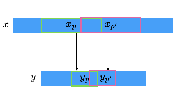
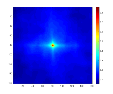
Figure 1: (Left) Between-locality in a sequence-to-sequence setting: each window (part) $y_{p}$ of the output sequence $y$ is fully determined by the part $x_{p}$ of the input sequence $x$, for every $p\in P$. (Right) Empirical within-locality $\mathsf{C}_{p,q}$ of $100$ images sampled from ImageNet between a $20\times 20$ patch $q$ and the central patch $p$.

Assumption 1 (Between-locality).

$y_{p}$ is conditionally independent from $x$, given $x_{p}$, moreover the probability of $y_{p}$ given $x_{p}$ is the same as $y_{q}$ given $x_{q}$, for any $p,q\in P$.

Between-locality (BL) assumes that the $p$-th part of the output $y\in Y$ depends only on the $p$-th part of the input $x\in X$, see Fig. 1 (Left) for an intuition in the case of sequence-to-sequence prediction. This is often verified in pixel-wise classification settings, where the class $y_{p}$ of a pixel $p$ is determined only by the sub-image in the corresponding patch $x_{p}$. BL essentially corresponds to assuming a joint graphical model on the parts of $x$ and $y$, where each $y_{p}$ is only connected to $x_{p}$ but not to other parts.

BL motivates us to focus on a local level by directly learning the relation between input-output parts. This is often an effective strategy in computer vision [20, 36, 16] but intuitively, one that provides significant advantages only when the input parts are not highly correlated with each other: in the extreme case where all parts are identical, there is no advantage in solving the learning problem locally. In this sense it can be useful to measure the amount of “covariance”

$$\mathsf{C}_{p,q}=\mathbb{E}_{x}\leavevmode\nobreak\ {S(x_{p},x_{q})}-\mathbb{E}_{x,x^{\prime}}\leavevmode\nobreak\ S(x_{p},x^{\prime}_{q})$$ (1)

between two parts $p$ and $q$ of an input $x$, for $S(x_{p},x_{q})$ a suitable measure of similarity between parts (if $S(x_{p},x_{q})=x_{p}x_{q}$, with $x_{p}$ and $x_{q}$ scalars random variables, then $\mathsf{C}_{p,q}$ is the $p,q$-th entry of the covariance matrix of the vector $(x_{1},\dots,x_{|P|})$ ). Here $\mathbb{E}_{x}S(x_{p},x_{q})$ and $\mathbb{E}_{x,x^{\prime}}S(x_{p},x^{\prime}_{q})$ measure the similarity between the $p$-th and the $q$-th part of, respectively, the same input, and two independent ones (in particular $\mathsf{C}_{p,q}=0$ when the $p$-th and $q$-th part of $x$ are independent). In many applications, it is reasonable to assume that $\mathsf{C}_{p,q}$ decays according to the distance between $p$ and $q$.

Assumption 2 (Within-locality).

There exists a distance $d:P\times P\to\mathbb{R}$ and $\gamma\geq 0$, such that

$$\left|\mathsf{C}_{p,q}\right|\leavevmode\nobreak\ \leqslant\leavevmode\nobreak\ {\mathsf{r}}^{2}\leavevmode\nobreak\ e^{-\gamma d(p,q)}\qquad\text{with}\qquad\mathsf{r}^{2}=\sup_{x,x^{\prime}}|S(x,x^{\prime})|.$$ (2)

Within-locality (WL) is always satisfied for $\gamma=0$. However, when $x_{p}$ is independent of $x_{q}$, it holds with $\gamma=\infty$ and $d(p,q)=\delta_{p,q}$ the Dirac’s delta. Exponential decays of correlation are typically observed when the distribution of the parts of $x$ factorizes in a graphical model that connects parts which are close in terms of the distance $d$: although all parts depend on each other, the long-range dependence typically goes to zero exponentially fast in the distance (see, e.g., [22] for mixing properties of Markov chains). Fig. 1 (Right) reports the empirical WL measured on $100$ images randomly sampled from ImageNet [13]: each pixel $(i,j)$ reports the value of $\mathsf{C}_{p,q}$ of the central patch $p$ with respect to a $20\times 20$ patch $q$ centered in $(i,j)$. Here $S(x_{p},x_{q})=x_{p}^{\top}x_{q}$. We note that $\mathsf{C}_{p,q}$ decreases extremely fast as a function of the distance $\bigl{\|}{p-q}\bigr{\|}$, suggesting that Assumption 2 holds with a large value of $\gamma$.

Contributions

In this work we present a novel structured prediction algorithm that adaptively leverages locality in the learning problem, when present (Sec. 4). We study the generalization properties of the proposed estimator (Sec. 5), showing that it is equivalent to the state of the art in the worst case scenario. More importantly, if the locality Assumptions 1 and 2 are satisfied, we prove that our learning rates improve proportionally to the number $|P|$ of parts in the problem. Here we give an informal version of this main result, reported in more detail in Thm. 4 (Sec. 5). Below we denote by ${\widehat{f}}$ the proposed estimator, by $\mathcal{E}(f)$ the expected risk of a function $f:X\to Y$ and ${f^{*}}=\operatornamewithlimits{argmin}_{f}\mathcal{E}(f)$.

Theorem 1 (Informal - Learning Rates & Locality).

Under mild assumptions on the loss and the data distribution, if the learning problem is local (Assumptions 1 and 2), there exists $c_{0}>0$ such that

$$\mathbb{E}\leavevmode\nobreak\ \left[\mathcal{E}({\widehat{f}}\leavevmode\nobreak\ )-\mathcal{E}({f^{*}})\right]\leavevmode\nobreak\ \leqslant\leavevmode\nobreak\ c_{0}\left(\frac{{\mathsf{s}}}{n|P|}\right)^{1/4},\qquad{\mathsf{s}}=\frac{\mathsf{r}^{2}}{|P|}\sum_{p,q=1}^{|P|}\leavevmode\nobreak\ e^{-\gamma d(p,q)},$$ (3)

where the expectation is taken with respect to the sample of $n$ input-output points used to train ${\widehat{f}}$.

In the worst-case scenario $\gamma=0$ (no exponential decay of the covariance between parts), the bound in 3 scales as $1/n^{1/4}$ (since ${\mathsf{s}}=\mathsf{r}^{2}|P|$) recovering [8], where no structure is assumed on the parts. However, as soon as $\gamma>0$, ${\mathsf{s}}$ can be upper bounded by a constant independent of $|P|$ and thus the rate scales as $1/(|P|n)^{1/4}$, accelerating proportionally to the number of parts. In this sense, Thm. 1 shows the significant benefit of making use of locality. The following example focuses on the special case of sequence-to-sequence prediction.

Example 1 (Locality on Sequences).

As depicted in Fig. 1, for discrete sequences we can consider parts (e.g., windows) indexed by $P=\{1,\dots,|P|\}$, with $d(p,q)=|p-q|$ for $p,q\in P$ (see Sec. K.1 for more details). In this case, Assumption 2 leads to

$${\mathsf{s}}\leavevmode\nobreak\ \leavevmode\nobreak\ \leqslant\leavevmode\nobreak\ \leavevmode\nobreak\ 2\mathsf{r}^{2}(1-e^{-\gamma})^{-1},$$ (4)

which for $\gamma>0$ is bounded by a constant not depending on the number of parts. Hence, Thm. 1 guarantees a learning rate of order $1/(n|P|)^{1/4}$, which is significanlty faster than the rate $1/n^{1/4}$ of methods that do not leverage locality such as [8]. See Sec. 6 for empirical support to this observation.

3 Problem Formulation

We denote by $X,Y$ and $Z$ respectively the input space, label space and output space of a learning problem. Let $\rho$ be a probability measure on $X\times Y$ and $\bigtriangleup:Z\times Y\times X\to\mathbb{R}$ a loss measuring prediction errors between a label $y\in Y$ and a output $z\in Z$, possibly parametrized by an input $x\in X$. To stress this interpretation we adopt the notation $\bigtriangleup(z,y|x)$. Given a finite number of $(x_{i},y_{i})_{i=1}^{n}$ independently sampled from $\rho$, our goal is to approximate the minimizer ${f^{*}}$ of the expected risk

$$\min_{f:X\to Z}\mathcal{E}(f),\quad\textrm{with}\quad\mathcal{E}(f)=\int\bigtriangleup(f(x),y|x)\leavevmode\nobreak\ d\rho(x,y).$$ (5)

Loss Made by Parts

We formalize the intuition introduced in Sec. 2 that data are decomposable into parts: we denote the sets of parts of $X,Y$ and $Z$ by respectively ${\left[X\right]},{\left[Y\right]}$ and ${\left[Z\right]}$. These are abstract sets that depend on the problem at hand (see examples below). We assume $P$ to be a set of part “indices” equipped with a selection operator $X\times P\to{\left[X\right]}$ denoted $(x,p)\mapsto[x]_{p}$ (analogously for $Y$ and $Z$). When clear from context, we will use the shorthand $x_{p}=[x]_{p}$. For simplicity, in the following we will assume $P$ be finite, however our analysis generalizes also to the infinite case (see supplementary material). Let $\pi(\cdot|x)$ be a probability distribution over the set of parts $P$, conditioned with respect to an input $x\in X$. We study loss functions $\bigtriangleup$ that can be represented as

$$\bigtriangleup(z,y|x)=\sum_{p\in P}\leavevmode\nobreak\ \pi(p|x)\leavevmode\nobreak\ L_{p}({{z}_{p}},{{y}_{p}}|\leavevmode\nobreak\ {{x}_{p}}).$$ (6)

The collection of $(L_{p})_{p\in P}$ is a family of loss functions $L_{p}:{\left[Z\right]}\times{\left[Y\right]}\times{\left[X\right]}\to\mathbb{R}$, each comparing the $p$-th part of a label $y$ and output $z$. For instance, in an image processing scenario, $L_{p}$ could measure the similarity between the two images at different locations and scales, indexed by $p$. In this sense, the distribution $\pi(p|x)$ allows to weigh each $L_{p}$ differently depending on the application (e.g., mistakes at large scales could be more relevant than at lower scales). Various examples of parts and concrete cases are illustrated in the supplementary material, here we report an extract.

Example 2 (Sequence to Sequence Prediction).

Let $X=A^{k}$, $Y=Z=B^{k}$ for two sets $A,B$ and $k\in\mathbb{N}$ a fixed length. We consider in this example parts that are windows of length $l\leqslant k$. Then $P=\{1,\dots,k-l+1\}$ where $p\in P$ indexes the window $x_{p}=(x^{(p)},\dots,x^{(p+l-1)})$, with $x\in X$, where we have denoted $x^{(s)}$ the $s$-th entry of the sequence $x\in X$, analogous definition for $y_{p},z_{p}$. Finally, we choose the loss $L_{p}$ to be the 0-1 distance between two strings of same length $L_{p}(z_{p},y_{p}|x)=\bm{1}(z_{p}\neq y_{p})$. Finally, we can choose $\pi(p|x)=1/|P|$, leading to a loss function $\bigtriangleup(z,y|x)=\frac{1}{|P|}\sum_{p\in P}\leavevmode\nobreak\ \bm{1}({{z}_{p}}\neq{{y}_{p}})$, which is common in the context of CRF [19].

Remark 1 (Examples of Loss Functions by Parts).

Several loss functions used in machine learning have a natural formulation in terms of 6. Notable examples are the Hamming distance [10, 33, 11], used in settings such as hierarchical classification [35], computer vision [24, 36, 32] or trajectory planning [25] to name a few. Also, loss functions used in natural language processing, such as the precision/recall and F$1$ score can be written in this form. Finally, we point out that multi-task learning settings [23] can be seen as problem by parts, with the loss corresponding to the sum of standard regression/classification loss functions (least-squares, logistic, etc.) over the tasks/parts.

Algorithm 1  

Algorithm 2 – Localized Structured Prediction

 

Input: training set $(x_{i},y_{i})_{i=1}^{n}$, distributions $\pi(\cdot|x)$ a reproducing kernel $k$ on $X\times P$, hyperparameter $\lambda>0$, auxiliary dataset size $m\in\mathbb{N}$.

 

Generate the auxiliary set $(\eta_{j},\chi_{j},p_{j})_{j=1}^{m}$:

 Sample $i_{j}\in U_{n}(\cdot)$. Set $\chi_{j}=x_{i_{j}}$.

 Sample $p_{j}\sim\pi(\cdot|\chi_{j})$. Set $\eta_{j}=[y_{i_{j}}]_{p_{j}}$.

 

Learn the coefficients for the map $\alpha$:

 Set ${\mathbf{K}}$ with ${\mathbf{K}}_{jj^{\prime}}\,=\,k((\chi_{j},p_{j}),(\chi_{j^{\prime}},p_{j^{\prime}}))$.

 $\mathbf{A}=({\mathbf{K}}+m\lambda I)^{-1}$.

 

Return the map $\alpha:(x,p)\mapsto\mathbf{A}\leavevmode\nobreak\ v(x,p)\in\mathbb{R}^{m}$

 with $v(x,p)_{j}=k\big{(}(\chi_{j},p_{j}),(x,p)\big{)}$.

4 Algorithm

In this section we introduce our estimator for structured prediction problems with parts. Our approach starts with an auxiliary step for dataset generation that explicitly extracts the parts from the data.

Auxiliary Dataset Generation

The locality assumptions introduced in Sec. 2 motivate us to learn the local relations between individual parts $p\in P$ of each input-output pair. In this sense, given a training dataset ${\cal D}=(x_{i},y_{i})_{i=1}^{n}$ a first step would be to extract a new, part-based dataset $\{(x_{p},p,y_{p})\leavevmode\nobreak\ |\leavevmode\nobreak\ (x,y)\in{\cal D},\leavevmode\nobreak\ p\in P\}$. However in most applications the cardinality $|P|$ of the set of parts can be very large (possibly infinite as we discuss in the Appendix) making this process impractical. Instead, we generate an auxiliary dataset by randomly sub-sampling $m\in\mathbb{N}$ elements from the part-based dataset. Concretely, for $j\in\{1,\dots,m\}$, we first sample $i_{j}$ according to the uniform distribution $U_{n}$ on $\{1,\dots,n\}$, set $\chi_{j}=x_{i_{j}}$, sample $p_{j}\sim\pi(\cdot\leavevmode\nobreak\ |\leavevmode\nobreak\ \chi_{j})$ and finally set $\eta_{j}=[y_{i_{j}}]_{p_{j}}$. This leads to the auxiliary dataset ${\cal D}^{\prime}=(\chi_{j},p_{j},\eta_{j})_{j=1}^{m}$, as summarized in the Generate routine of Alg. 2.

Estimator

Given the auxiliary dataset, we propose the estimator ${\widehat{f}}:X\to Z$, such that $\forall x\in X$

$${\widehat{f}}(x)=\operatornamewithlimits{argmin}_{z\in Z}\sum_{p\in P}\sum_{j=1}^{m}\alpha_{j}(x,p)\leavevmode\nobreak\ \Big{[}\pi(p|x)\leavevmode\nobreak\ L_{p}({{z}_{p}},\eta_{j}|{{x}_{p}})\Big{]}.$$ (7)

The functions $\alpha_{j}:X\times P\to\mathbb{R}$ are learned from the auxiliary dataset and are the fundamental components allowing our estimator to capture the part-based structure of the learning problem. Indeed, for any test point $x\in X$ and part $p\in P$, the value $\alpha_{j}(x,p)$ can be interpreted as a measure of how similar $x_{p}$ is to the $p_{j}$-th part of the auxiliary training point $\chi_{j}$. For instance, assume $\alpha_{j}(x,p)$ to be an approximation of the delta function that is $1$ when ${{x}_{p}}={{[\chi_{j}]}_{p_{j}}}$ and $0$ otherwise. Then,

$$\alpha_{j}(x,p)\leavevmode\nobreak\ L_{p}({{z}_{p}},\eta_{j}|{{x}_{p}})\leavevmode\nobreak\ \leavevmode\nobreak\ \approx\leavevmode\nobreak\ \leavevmode\nobreak\ \delta({{x}_{p}},[\chi_{j}]_{p_{j}})\leavevmode\nobreak\ L_{p}({{z}_{p}},\eta_{j}|{{x}_{p}}),$$ (8)

which implies essentially that

$$x_{p}\approx[\chi_{j}]_{p_{j}}\leavevmode\nobreak\ \leavevmode\nobreak\ \Longrightarrow\leavevmode\nobreak\ \leavevmode\nobreak\ z_{p}\approx\eta_{j}.$$ (9)

In other words, if the $p$-th part of test input $x$ and the $p_{j}$-th part of the auxiliary training input $\chi_{j}$ (i.e., the $p_{j}$-th part of the training input $x_{i_{j}}$) are deemed similar, then the estimator will encourage the $p$-th part of the test output $z$ to be similar to the auxiliary part $\eta_{j}$. This process is illustrated in Fig. 2 for an ideal computer vision application: for a given test image $x$, the $\alpha$ scores detect a similarity between the $p$-th patch of $x$ and the $p_{j}$-th patch of the training input $x_{i_{j}}$. Hence, the estimator will enforce the $p$-th patch of the output $z$ to be similar to the $p_{j}$-th patch of the training label $y_{i_{j}}$.

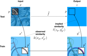
Figure 2: Illustration of the prediction process for the Localized Structured Prediction Estimator 7 for a hypothetical computer vision application.

Learning $\alpha$

In line with previous work on structured prediction [8], we learn each $\alpha_{j}$ by solving a linear system for a problem akin to kernel ridge regression (see Sec. 5 for the theoretical motivation). In particular, let $k:(X\times P)\times(X\times P)\to\mathbb{R}$ be a positive definite kernel, we define

$$(\alpha_{1}(x,p),\dots,\alpha_{m}(x,p))^{\top}=({\mathbf{K}}+m\lambda I)^{-1}v(x,p),$$ (10)

where ${\mathbf{K}}\in\mathbb{R}^{m\times m}$ is the empircal kernel matrix with entries ${\mathbf{K}}_{jh}=k((\chi_{j},p_{j}),(\chi_{h},p_{h}))$ and $v(x,p)\in\mathbb{R}^{m}$ is the vector with entries $v(x,p)_{j}=k((\chi_{j},p_{j}),(x,p))$. Training the proposed algorithm, consists in precomputing $\mathbf{A}=({\mathbf{K}}+m\lambda I)^{-1}$ to evaluate the coefficients $\alpha$ as detailed by the Learn routine in Alg. 2. While computing $\mathbf{A}$ amounts to solving a linear system, which requires $O(m^{3})$ operations, we note that it is possible to achieve the same statistical accuracy with reduced complexity $O(m\sqrt{m})$ by means of low rank approximations (see [14, 26]).

Remark 2 (Evaluating ${\widehat{f}}$).

According to (7), evaluating ${\widehat{f}}$ on a test point $x\in X$ consists in solving an optimization problem over the output space $Z$. This is a standard strategy in structured prediction, where an optimization protocol is derived on a case-by-case basis depending on both $\bigtriangleup$ and $Z$ (see, e.g., [24]). However, the specific form of our estimator suggests a general stochastic meta-algorithm to address this problem,. In particular, we can reformulate 7 as

$${\widehat{f}}(x)=\operatornamewithlimits{argmin}_{z\in Z}\leavevmode\nobreak\ \mathbb{E}_{j,p}\leavevmode\nobreak\ h_{j,p}(z|x),$$ (11)

with $p$ sampled according to $\pi$, $j\in\{1,\dots,m\}$ sampled according to the weights $\alpha_{j}$ and $h_{j,p}$ suitably defined in terms of $L_{p}$. When the $h_{j,p}$ are (sub)differentiable, (11) can be effectively addressed by stochastic gradient methods (SGM). In Alg. 4 in Appendix J we give an example of this strategy.

5 Generalization Properties of Structured Prediction with Parts

In this section we study the statistical properties for the proposed algorithm, with particular attention to the impact of locality on learning rates, see Thm. 4 (for a complete analysis of univeral consistency and learning rates without locality assumptions, see Appendices H and F). Our analysis leverages the assumption that the loss function $\bigtriangleup$ is a Structure Encoding Loss Function (SELF) by Parts.

Definition 1 (SELF by Parts).

A function $\bigtriangleup:Z\times Y\times X\to\mathbb{R}$ is a Structure Encoding Loss Function (SELF) by Parts if it admits a factorization in the form of (6) with functions $L_{p}:{\left[Z\right]}\times{\left[Y\right]}\times{\left[X\right]}\to\mathbb{R}$, and there exists a separable Hilbert space ${\mathcal{H}}$ and two bounded maps $\psi:{\left[Z\right]}\times{\left[X\right]}\times P\to{\mathcal{H}}$, $\varphi:{\left[Y\right]}\to{\mathcal{H}}$ such that for any $\zeta\in{\left[Z\right]}$, $\eta\in{\left[Y\right]}$, $\xi\in{\left[X\right]}$, $p\in P$

$$L_{p}(\zeta,\eta|\xi)\leavevmode\nobreak\ \leavevmode\nobreak\ =\leavevmode\nobreak\ \leavevmode\nobreak\ \left\langle{\psi(\zeta,\xi,p)},{\varphi(\eta)}\right\rangle_{\mathcal{H}}.$$ (12)

The definition of “SELF by Parts” specializes the definition of SELF in [9] and in the following we will always assume $\bigtriangleup$ to satisfy it. Indeed, Def. 1 is satisfied when the spaces of parts involved are discrete sets and it is rather mild in the general case (see [8] for an exhaustive list of examples). Note that when $\bigtriangleup$ is SELF, the solution of 5 is completely characterized in terms of the conditional expectation (related to the conditional mean embedding [7, 21, 28]) of $\varphi(y_{p})$ given $x$, denoted by ${g^{*}}:X\times P\to{\mathcal{H}}$, as follows.

Lemma 2.

Let $\bigtriangleup$ be SELF and $Z$ compact. Then, the minimizer of 5 is ${\rho_{X}}$-a.e. characterized by

$${f^{*}}(x)=\operatornamewithlimits{argmin}_{z\in Z}\sum_{p\in P}\pi(p|x)\left\langle{\psi(z_{p},x_{p},p)},{{g^{*}}(x,p)}\right\rangle_{\mathcal{H}},\qquad{g^{*}}(x,p)=\int_{Y}\varphi(y_{p})d\rho(y|x).$$ (13)

Lemma 2 (proved in Appendix C) shows that ${f^{*}}$ is completely characterized in terms of the conditional expectation ${g^{*}}$, which indeed plays a key role in controlling the learning rates of ${\widehat{f}}$. In particular, we investigate the learning rates in light of the two assumptions of between- and within-locality introduced in Sec. 2. To this end, we first study the direct effects of these two assumptions on the learning framework introduced in this work.

The effect of Between-locality

We start by observing that the between-locality between parts of the inputs and parts of the output allows for a refined characterization of the conditional mean ${g^{*}}$.

Lemma 3.

Let ${g^{*}}$ be defined as in 13. Under Assumption 1, there exists ${\bar{g}^{*}}:{\left[X\right]}\to{\mathcal{H}}$ such that

$${g^{*}}(x,p)={\bar{g}^{*}}(x_{p})\qquad\qquad\forall x\in X,\leavevmode\nobreak\ p\in P.$$ (14)

Lemma 3 above shows that we can learn ${g^{*}}$ by focusing on a “simpler” problem, identified by the function ${\bar{g}^{*}}$ acting only the parts ${\left[X\right]}$ of $X$ rather than on the whole input directly (for a proof see Lemma 21 in Appendix G). This motivates the adoption of the restriction kernel [6], namely a function $k:(X\times P)\times(X\times P)\to\mathbb{R}$ such that

$$k((x,p),(x^{\prime},q))=\bar{k}(x_{p},x_{q}),$$ (15)

which, for any pair of inputs $x,x^{\prime}\in X$ and parts $p,q\in P$, measures the similarity between the $p$-part of $x$ and the $q$-th part of $q$ via a kernel $\bar{k}:{\left[X\right]}\times{\left[X\right]}\to\mathbb{R}$ on the parts of $X$. The restriction kernel is a well-established tool in structured prediction settings [6] and it has been observed to be remarkably effective in computer vision applications [20, 36, 16].

The effect of Within-locality

We recall that within-locality characterizes the statistical correlation between two different parts of the input (see Assumption 2). To this end we consider the simplified scenario where the parts are sampled from the uniform distribution on $P$, i.e., $\pi(p|x)=\frac{1}{|P|}$ for any $x\in X$ and $p\in P$. While more general situations can be considered, this setting is useful to illustrate the effect we are interested in this work. We now define some important quantities that characterize the learning rates under locality,

$$\mathsf{C}_{p,q}=\mathbb{E}_{x,x^{\prime}}\left[\leavevmode\nobreak\ \bar{k}(x_{p},x_{q})^{2}-\bar{k}(x_{p},x^{\prime}_{q})^{2}\leavevmode\nobreak\ \right],\qquad\mathsf{r}=\sup_{x\in X,p\in P}\bar{k}(x_{p},x_{p}).$$ (16)

It is clear that the terms $\mathsf{C}_{p,q}$ and $\mathsf{r}$ above correspond respectively to the correlations introduced in 1 and the scale parameter introduced in 2, with similarity function $S=\bar{k}^{2}$. Let ${\widehat{f}}$ be the structured prediction estimator in 7 learned using the restriction kernel in 15 based on $\bar{k}$ and denote by $\bar{{\cal G}}$ the space of functions $\bar{{\cal G}}={\mathcal{H}}\otimes\bar{{\mathcal{F}}}$ with $\bar{{\mathcal{F}}}$ the reproducing kernel Hilbert space [3] associated to $\bar{k}$. In particular, in the following we will consider the standard assumption in the context of non-parametric estimation [7] on the regularity of the target function, which in our context reads as ${\bar{g}^{*}}\in\bar{{\cal G}}$. Finally we introduce $\mathsf{c}_{\bigtriangleup}^{2}=\sup_{z\in Z,x\in X}\frac{1}{|P|}\sum_{p\in P}\|\psi(z,x,p)\|_{\mathcal{H}}^{2}$ to measure the “complexity” of the loss $\bigtriangleup$ w.r.t. the representation induced by SELF decomposition (Def. 1) analogously to Thm. 2 of [8].

Theorem 4 (Learning Rates & Locality).

Under Assumptions 1 and 2 with $S=\bar{k}^{2}$, let ${\bar{g}^{*}}$ satisfying Lemma 3, with $\bar{\mathsf{g}}=\|{\bar{g}^{*}}\|_{\bar{{\cal G}}}<\infty$. Let ${\mathsf{s}}$ be as in 3. When $\lambda=(\mathsf{r}^{2}/m+{\mathsf{s}}/(|P|n))^{1/2}$, then

$$\mathbb{E}\leavevmode\nobreak\ {\cal E}({\widehat{f}}\leavevmode\nobreak\ )-{\cal E}({f^{*}})\leavevmode\nobreak\ \leqslant\leavevmode\nobreak\ 12\leavevmode\nobreak\ {\mathsf{c}_{\bigtriangleup}}\leavevmode\nobreak\ \mathsf{\bar{g}}\leavevmode\nobreak\ \left(\frac{\mathsf{r}^{2}}{m}+\frac{\mathsf{r}^{2}}{|P|n}+\frac{{\mathsf{s}}}{|P|n}\right)^{1/4}.$$ (17)

The proof of the result above can be found in Sec. G.1. We can see that between- and within-locality allow to refine (and potentially improve) the bound of $n^{-1/4}$ from structured prediction without locality [8] (see also Thm. 5 in Appendix F). In particular, we observe that the adoption of the restriction kernel in Thm. 4 allows the structured prediction estimator to leverage the within-locality, gaining a benefit proportional to the magnitude of the parameter $\gamma$. Indeed $\mathsf{r}^{2}\leqslant{\mathsf{s}}\leqslant\mathsf{r}^{2}|P|$ by definition. More precisely, if $\gamma=0$ (e.g., all parts are identical copies) then ${\mathsf{s}}=\mathsf{r}^{2}|P|$ and we recover the rate of $O(n^{-1/4})$ of [8], while if $\gamma$ is large (the parts are almost not correlated) then ${\mathsf{s}}=\mathsf{r}^{2}$ and we can take $m\propto n|P|$ achieving a rate of the order of $O\big{(}(n|P|)^{-1/4}\big{)}$. We clearly see that depending on the amount of within-locality in the learning problem, the proposed estimator is able to gain significantly in terms of finite sample bounds.

6 Empirical Evaluation

We evaluate the proposed estimator on simulated as well as real data. We highlight how locality leads to improved generalization performance, in particular when only few training examples are available.

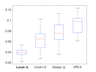
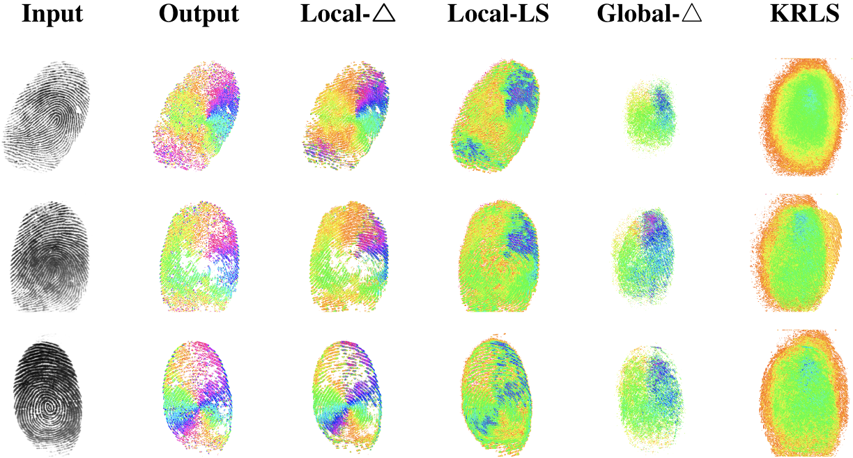
Figure 3: Learning the direction of ridges in fingerprint images. (Left) Examples of ground truths and predictions with pixels’ color corresponding to the local direction of ridges. (Right) Test error according to $\bigtriangleup$ in 18.

Learning the Direction of Ridges for Fingerprint

Similarly to [29], we considered the problem of detecting the pointwise direction of ridges in a fingerprint image on the FVC04 dataset comprising $80$ grayscale $640\times 480$ input images depicting fingerprints and corresponding output images encoding in each pixel the local direction of the ridges of the input fingerprint as an angle $\theta\in[-\pi,\pi]$. A natural loss function is the average pixel-wise error $\sin(\theta-\theta^{\prime})^{2}$ between a ground-truth angle $\theta$ and the predicted $\theta^{\prime}$ according to the geodesic distance on the sphere. To apply the proposed algorithm, we consider the following representation of the loss in term of parts: let $P$ be the collection of patches of dimension $20\times 20$ and equispaced each $5\times 5$ pixels so that each pixel belongs exactly to $16$ patches. For all $z,y\in\mathbb{R}^{640\times 480}$, the average pixel-wise error is

$$\bigtriangleup(z,y)=\frac{16}{|P|}\sum_{p\in P}L(z_{p},y_{p}),\qquad\text{with}\qquad L(\zeta,\eta)=\frac{1}{20\times 20}\sum_{i,j=1}^{20}\sin([\zeta]_{ij},[\eta]_{ij})^{2},$$ (18)

where $\zeta=z_{p},\eta=y_{p}\in[-\pi,\pi]^{20\times 20}$ are the extracted patches and $[\cdot]_{ij}$ their value at pixel $(i,j)$.

We compared our approach using $\bigtriangleup$ (Local-$\bigtriangleup$) or least-squares (Local-LS) with competitors that do not take into account the local structure of the problem, namely standard vector-valued kernel ridge regression (KRLS) [7] and the structured prediction algorithm in [8] with $\bigtriangleup$ loss ($\bigtriangleup$-Global). We used a Gaussian kernel on the input (for the local estimators the restriction kernel in 15 with $\bar{k}$ Gaussian). We randomly sampled $50/30$ images for training/testing, performing $5$-fold cross-validation on $\lambda$ in $[10^{-6},10]$ (log spaced) and the kernel bandwidth in $[10^{-3},1]$. For Local-$\bigtriangleup$ and Local-LS we built an auxiliary set with $m=30000$ random patches (see Sec. 4), sampled from the $50$ training images.

Results

Fig. 3 (Left) reports the average prediction error across $10$ random train-test splits. We make two observations: first, methods that leverage the locality in the data are consistently superior to their “global” counterparts, supporting our theoretical results in Sec. 5 that the proposed estimator can lead to significantly better performance, in particular when few training points are available. Second, the experiment suggests that choosing the right loss is critical, since exploiting locality without the right loss (i.e., Local-LS in the figure) generally leads to worse performance. The three sample predictions in Fig. 3 (Right) provide more qualitative insights on the models tested. In particular while both locality-aware methods are able to recover the correct structure of the fingerprints, only combining this information with the loss $\bigtriangleup$ leads to accurate recovery of the ridge orientation.

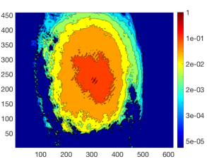
Figure 4: Empirical estimation of within-locality for the central patch of the fingerprints dataset.

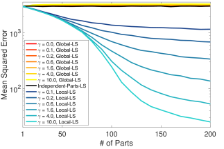
Figure 5: Effect of within-locality w.r.t. $\gamma$ and $|P|$: Global-LS vs. IndependentParts-LS vs. Local-LS (ours).

Within-locality

In Fig. 5 we visualize the (empirical) within-locality of the central patch $p$ for the fingerprint dataset. The figure depicts $\mathsf{C}_{p,q}$ (defined in 16) for $q\in P$, with the $(i,j)$-th pixel in the image corresponding to $\mathsf{C}_{p,q}$ with $q$ the $20\times 20$ patch centered in $(i,j)$. The fast decay of these values as the distance from the central patch $p$ increase, suggests that within-locality holds for a large value of $\gamma$, possibly justifying the good performance exhibited by (Local-$\bigtriangleup$) in light of Thm. 4.

Simulation: Within-Locality

We complement our analysis with synthetic experiments where we control the “amount” of within-locality $\gamma$. We considered a setting where input points are vectors $x\in\mathbb{R}^{k|P|}$ comprising $|P|$ parts of dimension $k=1000$. Inputs are sampled according to a normal distribution with zero mean and covariance $\Sigma(\gamma)=M(\gamma)\otimes I$, where $M(\gamma)\in\mathbb{R}^{|P|\times|P|}$ has entries $M(\gamma)_{pq}=\textnormal{e}^{-\gamma d(p,q)}$ and $d(p,q)=|p-q|/|P|$. By design, as $\gamma$ grows $\mathsf{C}$ varies from being rank-one (all parts are identical copies) to diagonal (all parts are independently sampled).

To isolate the effect of within-locality on learning, we tested our estimator on a linear multitask (actually vector-valued) regression problem with least-squares loss $\bigtriangleup$. We generated datasets $(x_{i},y_{i})_{i=1}^{n}$ of size $n=100$ for training and $n=1000$ for testing, with $x_{i}$ sampled as described above and $y_{i}=w^{\top}x_{i}+\epsilon$ with noise $\epsilon\in\mathbb{R}^{k|P|}$ sampled from an isotropic Gaussian with standard deviation $0.5$. To guarantee between-locality to hold, we generated the target vector $w=[\bar{w},\dots,\bar{w}]\in\mathbb{R}^{k|P|}$ by concatenating copies of a $\bar{w}\in\mathbb{R}^{k}$ sampled uniformly on the radius-one ball. We performed regression with linear restriction kernel on the parts/subvectors (Local-LS) on the “full” auxiliary dataset $([x_{i}]_{p},[y_{i}]_{p})$ with $1\leqslant i\leqslant n$ and $1\leqslant p\leqslant|P|$, and compared it with standard linear regression (Global-LS) on the original dataset $(x_{i},y_{i})_{i=1}^{n}$ and linear regression performed independently for each (local) subdataset $([x_{i}]_{p},[y_{i}]_{p})_{i=1}^{n}$ (IndependentParts - LS). The parameter $\lambda$ was chosen by hold-out cross-validation in $[10^{-6},10]$ (log spaced).

Fig. 5 reports the (log scale) mean square error (MSE) across $100$ runs of the two estimators for increasing values of $\gamma$ and $|P|$. In line with Thm. 4, when $\gamma$ and $|P|$ are large, Local-LS significantly outperforms both $i)$ Global-LS, which solves one single problem jointly and does not benefit within-locality, and $ii)$ IndependentParts-LS, which is insensitive to the between-locality across parts and solves each local prediction problem in isolation. For a smaller $\gamma$, such advantage becomes less prominent even when the number of parts is large. This is expected since for $\gamma=0$ the input parts are extremely correlated and there is no within locality that can be exploited.

7 Conclusion

We proposed a novel approach for structured prediction in presence of locality in the data. Our method builds on [8] by incorporating knowledge of the parts directly within the learning model. We proved the benefits of locality by showing that, under a low-correlation assumption on the parts of the input (within locality), the learning rates of our estimator can improve proportionally to the number of parts in the data. To obtain this result we additionally introduced a natural assumption on the conditional independence between input-output parts (between locality), which provides also a formal justification for adoption of the so-called “restriction kernel”, previously proposed in the literature, as a mean to lower the sample complexity of the problem. Empirical evaluation on synthetic as well as real data shows that our approach offers significant advantages when few training points are available and leveraging structural information such as locality is crucial to achieve good prediction performance. We identify two main directions for future work: $1)$ consider settings where the parts are unknown (or “latent”) and need to be discovered/learned from data; $2)$ Consider more general locality assumptions. In particular, we argue that Assumption 2 (WL) might be weakened to account for different (but related) local input-output relations across adjacent parts.

Appendix

In this appendix we provide further background to the main discussion and results in the main sections of the current work. In particular:

• Appendix A introduces a generalization of the proposed framework to account for a larger family of structured prediction problems where locality can be exploited.

• Appendix B introduces the notation and auxiliary results that will be useful to prove the results discussed in this work.

• Appendix C discusses the derivation of the structured prediction estimator proposed and studied in this work.

• Appendix D extends the Comparison inequality for the SELF estimator in [8] to the case where the locality of the problem can be exploited.

• Appendix E provides an analytical decomposition of a bound for the excess risk of the proposed estimator that is then used to prove the learning rates of the proposed estimator without and with parts (respectively Appendices F and G) and also the universal consistency (Appendix H).

• Appendix I compares the proposed framework with structured prediction (without parts) in [8].

• Appendix J provides more details on the problem of learning and evaluating the estimator proposed in this work.

• Appendix K discusses in more detail loss functions considered in the literature that can be decomposed into “parts”.

An overview of the main result in Thm. 4

For the sake of clarity, before delving in the discussion below, we discuss here how the main result of this work, namely Thm. 4, is situated within the appendix. While the formal proof is given in Sec. G.1, here we highlight and reference the key results used to this purpose. The main analysis in this sense can be found in Appendices E, F and G. In particular, the proof hinges on three main components:

1. We begin by studing the conditional expectation ${g^{*}}$ introduced in Lemma 2 in terms of an estimator ${\widehat{g}}$. In Appendices C and D we prove that this estimator is tightly connected to our structured prediction estimator in 7 according to the comparison inequality

   $$\mathcal{E}({\widehat{f}}\leavevmode\nobreak\ )-\mathcal{E}({f^{*}})\leqslant{\mathsf{c}_{\bigtriangleup}}\|{\widehat{g}}-{g^{*}}\|_{{L^{2}(X\times P,\pi{\rho_{X}},{\mathcal{H}})}}.$$ (19)

   proved in Thm. 9 in Appendix D.

2. The inequality above suggest to focus on $\|{\widehat{g}}-{g^{*}}\|_{{L^{2}(X\times P,\pi{\rho_{X}},{\mathcal{H}})}}$. We do this by providing an analytic decomposition for this quantity in Thm. 11 in Appendix E.

3. Finally, in Appendix F we consider how each term in such analytical decomposition can be controlled in expectation with respect to a training dataset randomly sampled from the underlying distribution $\rho$.

Putting together all these results we are able to characterize the excess risk bounds for our estimator ${\widehat{f}}$ in the general setting where locality does not necessary hold, which is reported below and proved at the end of Sec. F.3.

Theorem 5.

Let ${\widehat{f}}$ as in 7 with i.i.d. training set and auxiliary dataset sampled according to Alg. 2. Let $\bigtriangleup$ be SELF, $Z$ compact, $g^{*}\in{\cal G}$ and $\lambda\geq(\mathsf{r}^{2}/m+\mathsf{q}/n)^{1/2}$. Then

$$\mathbb{E}\leavevmode\nobreak\ \left[\mathcal{E}({\widehat{f}}\leavevmode\nobreak\ )-\mathcal{E}({f^{*}})\right]\leavevmode\nobreak\ \leqslant\leavevmode\nobreak\ 12\leavevmode\nobreak\ {\mathsf{c}_{\bigtriangleup}}\leavevmode\nobreak\ \mathsf{g}\leavevmode\nobreak\ \left(\frac{\mathsf{r}^{2}}{\lambda m}+\frac{\mathsf{q}}{\lambda n}+\lambda\right)^{1/2}.$$ (20)

Here we have introduced the quantity

$$\begin{split}\mathsf{q}=\mathbb{E}_{x,x^{\prime}}\mathbb{E}_{p,q|x,r|x^{\prime}}\leavevmode\nobreak\ \leavevmode\nobreak\ \mathsf{C}_{p,q}(x,x^{\prime})\qquad\mathsf{C}_{p,q}(x,x^{\prime})=\left[k((x,p),(x,q))^{2}-k((x,p),(x^{\prime},r))^{2}\right],\end{split}$$ (21)

where $\mathbb{E}_{p,q|x}[\cdot]$ is a shorthand for $\sum_{p,q\in P}\pi(p|x)\pi(q|x)[\cdot]$ (analogously for $\mathbb{E}_{r|x}$). It can be seen that this quantity allows to capture and leverage the within-locality assumption. In particular, it will allow us to quantify explicitly the advantages of using our locality-aware estimator.

The result above explicitly shows how the quantities measuring the within locality do affect the constants in the learning rates of the proposed estimator. By combining Thm. 5 with Assumptions 1 and 2 and leveragin the locality properties of the restriction kernel introduced in 15, we are then able to prove Thm. 4 as desired. As mentioned, the details of this proof are reported in Sec. G.1.

Appendix A Generalization of the Model by Parts

In this section we introduce a slight generalization of the model considered in this work and that will be used in the rest of the appendixes. In particular we consider the case where $P$ is not necessarily finite and, possibly, the observed parts of $y$ are not necessarily deterministic.

A.1 When the Parts don’t correspond exactly

In general, $y_{p}$ (the $p$-th part of $y$) could not be univocally determined given $p\in P$. For instance, consider a speech recognition problem where the goal is to predict the sentence pronounced by a speaker from an audio signal. In this setting the input space $X$ is the set of all audio signals and $Y=Z$ is the set of all strings that can be produced in the speaker’s language. In principle, for any part $x_{p}$ of an input signal $x\in X$ it is possible to identify the corresponding part $y_{p}$ of the target string. In practice, such a procedure would require significant preprocessing (e.g. using hidden markov models) and would however not be guaranteed to be error-free.

In general, given an input $x\in X$ a label $y\in Y$ and a part $p\in P$, observations for the $p$-th part of $y$ can be distributed according to some probability $\mu(w|y,x,p)$ over the set ${\left[Y\right]}$ of parts of $Y$. A possible way to model this situation is to consider a characterization of $L$ in terms of a further function $\ell:Z\times{\left[Y\right]}\times X\times P\to\mathbb{R}$ such that

$$\bigtriangleup(z,y|x) =\int_{P}L(z,y|x,p)d\pi(p|x),\leavevmode\nobreak\ \leavevmode\nobreak\ \textrm{where}\leavevmode\nobreak\ \leavevmode\nobreak\$$ (22)

$$L(z,y|x,p) =\int_{\left[Y\right]}\ell(z,\eta|x,p)\leavevmode\nobreak\ d\mu(\eta|y,x,p).$$ (23)

In this sense, the distribution $\mu$ can be interpreted as characterizing how likely it is for the part $p$ of an input $x$ with associated label $y$ to correspond to $\eta\in{\left[Y\right]}$. It is possible to recover the standard characterization by selecting $\mu$ to be the Dirac de

$$\mu(\eta|y,x,p)=\delta(\eta,y_{p}).$$

Remark 3 (Connection with standard Structured Prediction).

Note that the loss above generalizes the standard structured prediction framework as in [34, 24, 8]. Indeed, it is always possible to formulate a structured prediction loss $\bigtriangleup$ in the proposed setting, by taking $\ell=\bigtriangleup$ and $P=\{0\}$, ${\left[Y\right]}=Y$, $\pi(0|x)=1$ and $\mu(w|y,x,0)=\delta_{y}$. However, if there exists a non-trivial characterization of $\bigtriangleup$ in terms of these objects, then the algorithm proposed in this work is able to exploit this additional structure to achieve improved generalization performance.

Here we give the extended defintion of the SELF assumption, given the definition of loss in 22.

Definition 2 (SELF by Parts (Extended)).

A function $\bigtriangleup:Z\times Y\times X\to\mathbb{R}$ is a Structure Encoding Loss Function (SELF) by Parts if it admits a factorization in the form of (22) with functions $\ell:Z\times{\left[Y\right]}\times X\times P\to\mathbb{R}$, and there exists a separable Hilbert space ${\mathcal{H}}$ and two bounded continuous maps $\psi:{\left[Z\right]}\times{\left[X\right]}\times P\to{\mathcal{H}}$, $\varphi:{\left[Y\right]}\to{\mathcal{H}}$ such that for any $z\in Z$, $\eta\in{\left[Y\right]}$, $x\in X$, $p\in P$

$$\ell(z,\eta|x,p)=\left\langle{\psi(z,x,p)},{\varphi(\eta)}\right\rangle_{\mathcal{H}}.$$ (24)

Remark 4 (Def. 2 is more general than Def. 1).

Given a loss $\bigtriangleup$ satisfying Def. 1 for some $\psi^{\prime},\phi,{\mathcal{H}}^{\prime}$, then it satisfy Def. 2, with $\psi(z,x,p)=\psi^{\prime}(z_{p},z_{p},p)$, with $\phi=\phi^{\prime}$ with ${\mathcal{H}}={\mathcal{H}}^{\prime}$.

Appendix B Notation and Main Definitions

Let ${L^{2}(X\times P,\pi{\rho_{X}})}$ be the Lebesgue function space with norm

$$\|\beta\|_{{L^{2}(X\times P,\pi{\rho_{X}})}}^{2}=\int_{X\times P}\beta(x,p)^{2}\leavevmode\nobreak\ d\pi(p|x)d{\rho_{X}}(x)$$

with $\beta:X\times P\to\mathbb{R}$. Analogously, ${L^{2}(X\times P,\pi{\rho_{X}},{\mathcal{H}})}$ be the Lebesgue function space with norm

$$\|\beta\|_{{L^{2}(X\times P,\pi{\rho_{X}},{\mathcal{H}})}}^{2}=\int_{X\times P}\|\beta(x,p)\|_{\mathcal{H}}^{2}\leavevmode\nobreak\ d\pi(p|x)d{\rho_{X}}(x)$$

with $\beta:X\times P\to{\mathcal{H}}$. Let $\big{(}(x_{i},y_{i})\big{)}_{i=1}^{n}$ be the training set and let $\big{(}(x_{i_{j}},y_{i_{j}},p_{j},w_{j})\big{)}_{j=1}^{m}$. Denote with ${\widehat{\rho}_{X}}$ the probability measure $\frac{1}{n}\sum_{i=1}^{n}\delta_{x_{i}}$. We define ${L^{2}(X\times P,\pi{\widehat{\rho}_{X}},{\mathcal{H}})}$ the Lebesgue function space with norm

$$\|\beta\|_{{L^{2}(X\times P,\pi{\widehat{\rho}_{X}},{\mathcal{H}})}}^{2}=\frac{1}{n}\sum_{i=1}^{n}\int_{P}\|\beta(x_{i},p)\|_{\mathcal{H}}^{2}\leavevmode\nobreak\ d\pi(p|x_{i}).$$

with $\beta:X\times P\to{\mathcal{H}}$.

Let $k:(X\times P)\times(X\times P)\to\mathbb{R}$ be a reproducing kernel with associated reproducing kernel Hilbert space (RKHS) ${\mathcal{F}}$. For any $(x,p)\in X\times P$ we denote $k_{x,p}=k\big{(}(x,p),\cdot\big{)}\in{\mathcal{F}}$.

We introduce the following objects:

• $S:{\mathcal{F}}\to{L^{2}(X\times P,\pi{\rho_{X}})}$   the operator such that, for any $f\in{\mathcal{F}}$,

  $$(Sf)(\cdot,\cdot)=\left\langle{f},{k_{(\cdot,\cdot)}}\right\rangle_{\mathcal{F}}.$$

• $S^{*}:{L^{2}(X\times P,\pi{\rho_{X}})}\to{\mathcal{F}}$   the operator such that, for any $\beta\in{L^{2}(X\times P,\pi{\rho_{X}})}$,

  $${S^{*}\beta=\int_{X\times P}k_{x,p}\beta(x,p)\leavevmode\nobreak\ d\pi(p|x)d{\rho_{X}}(x)}.$$

• $C:{\mathcal{F}}\to{\mathcal{F}}$ the operator $\displaystyle{C=\int_{X\times P}k_{x,p}\otimes k_{x,p}\leavevmode\nobreak\ d\pi(p|x)d{\rho_{X}}(x)}$.

• ${\widetilde{C}}:{\mathcal{F}}\to{\mathcal{F}}$ the operator $\displaystyle{{\widetilde{C}}=\frac{1}{n}\sum_{i=1}^{n}\int_{P}k_{x_{i},p}\otimes k_{x_{i},p}\leavevmode\nobreak\ d\pi(p|x_{i})}$.

• ${\widehat{C}}:{\mathcal{F}}\to{\mathcal{F}}$ the operator $\displaystyle{{\widehat{C}}=\frac{1}{m}\sum_{j=1}^{m}k_{x_{i_{j}},p_{j}}\otimes k_{x_{i_{j}},p_{j}}}$.

• $L:{L^{2}(X\times P,\pi{\rho_{X}})}\to{L^{2}(X\times P,\pi{\rho_{X}})}$ the operator such that for any $\beta\in{L^{2}(X\times P,\pi{\rho_{X}})}$, we have that $(L\beta)(\cdot)=\int_{X\times P}k\big{(}(x,p),\cdot\big{)}\beta(x,p)\leavevmode\nobreak\ d\pi(p|x)d{\rho_{X}}(x)$.

• $B:{\mathcal{H}}\to{\mathcal{F}}$ the operator $B=\int_{P\times X}k_{x,p}\otimes\varphi(w)\leavevmode\nobreak\ d\mu(w|y,x,p)d\pi(p|x)d\rho(y,x)$. Note that by definiton $B=\int k_{x,p}\otimes{g^{*}}(x,p)\leavevmode\nobreak\ d\pi(p|x)d\rho_{X}(x)$ with ${g^{*}}$ defined as in 13.

• ${\widehat{B}}:{\mathcal{H}}\to{\mathcal{F}}$ the operator ${\widehat{B}}=\frac{1}{m}\sum_{j=1}^{m}k_{x_{i_{j}},p_{j}}\otimes\varphi(w_{j})$.

• $G:{\mathcal{H}}\to{L^{2}(X\times P,\pi{\rho_{X}})}$ the operator such that, for any $h\in{\mathcal{H}}$ is such that $(Gh)(\cdot)=\left\langle{{g^{*}}(\cdot)},{h}\right\rangle_{\mathcal{H}}$ for any $h\in{\mathcal{H}}$, with ${g^{*}}$ defined as in 13.

Further Notation

Let ${\mathcal{H}}$ and ${\mathcal{F}}$ be two Hilbert spaces and let $h\in{\mathcal{H}}$ and $f\in{\mathcal{F}}$, we denote with $h\otimes f$ the bounded linear operator from ${\mathcal{F}}\to{\mathcal{H}}$ such that, for any $g\in{\mathcal{F}}$, we have $(h\otimes f)g=h\left\langle{f},{g}\right\rangle_{\mathcal{F}}$. Note that $h\otimes f\in{\mathcal{H}}\otimes{\mathcal{F}}$, where ${\mathcal{H}}\otimes{\mathcal{F}}$ is the tensor product between the Hilbert spaces ${\mathcal{H}},{\mathcal{F}}$ and is isometric to the the space of Hilbert-Schmidt operators from ${\mathcal{F}}$ to ${\mathcal{H}}$, denoted by ${\rm HS}({\mathcal{F}},{\mathcal{H}})$, namely the bounded linear operators $G:{\mathcal{F}}\to{\mathcal{H}}$ with finite Hilbert-Schmidt norm $\|G\|_{\rm HS}=\sqrt{\text{\rm Tr}(G^{*}G)}$.

B.1 Auxiliary Results

Lemma 6.

With the notation introduced above, the following equations hold.

• $L=SS^{*}$.

• $C=S^{*}S$.

• $SC_{\lambda}^{-1}S^{*}=LL_{\lambda}^{-1}=I-\lambda L_{\lambda}^{-1}$.

• $C_{\lambda}^{-1}S^{*}=S^{*}L_{\lambda}^{-1}$.

• $\|C_{\lambda}^{-1/2}S^{*}\|=\|S^{*}L_{\lambda}^{-1/2}\|\leqslant 1$ for any $\lambda>0$

The proof of the result above are well known and we refer to Appendix B in [8] for a proof with same notation as the one adopted in this paper. Below we show two further results that we will need

Lemma 7.

with the notation introduced above we have

$$B=S^{*}G.$$ (25)

Proof.

By applying the definition of the two operators $S$ and $G$ we have that for any $h\in{\mathcal{H}}$,

$$S^{*}Gh =S^{*}\big{(}(Gh)(\cdot)\big{)}$$ (26)

$$=S^{*}(\left\langle{g^{*}(\cdot)},{h}\right\rangle_{\mathcal{H}})$$ (27)

$$=\int k_{x,p}\left\langle{{g^{*}}(x,p)},{h}\right\rangle_{\mathcal{H}}\leavevmode\nobreak\ d\pi(p|x)d{\rho_{X}}(x)$$ (28)

$$=\int(k_{x,p}\otimes{g^{*}}(x,p))h\leavevmode\nobreak\ d\pi(p|x)d{\rho_{X}}(x)=Bh$$ (29)

Hence $B=S^{*}G$ as required. ∎

Appendix C Derivation of the algorithm

In this section we show how the algorithm naturally derives from the definition of the problem and in particular we prove Lemma 2. Our analysis starts from the observation that when the loss function is SELF the solution of the learning problem in 5 is completely characterized in terms of the conditional expectation of $\varphi(y_{p})$ given $x$, denoted by ${g^{*}}:X\times P\to{\mathcal{H}}$, with

$${g^{*}}(x,p)=\int\varphi(\eta)d\mu(\eta|x,y,p)d\rho(y|x).$$ (30)

Note that since $\varphi(\cdot)$ is bounded and continuous, we have that ${g^{*}}\in{L^{2}}(X,\pi{\rho_{X}},{\mathcal{H}})$. Below we prove Lemma 2

See 2

Proof.

By Berge maximum theorem[2] (see also [8]), since $Z$ is compact, we have that the solution of the learning problem in 5 is characterized by

$${f^{*}}(x)=\operatornamewithlimits{argmin}_{z\in Z}\int\bigtriangleup(z,y|x)d\rho(y|x).$$

The result is obtained by expanding the definition of $\bigtriangleup$ with respect to SELF (Def. 2) and the linearity of the inner product and the integral

$$\int\bigtriangleup(z,y|x)d\rho(y|x) =\int\ell(z,\eta|x,p)d\mu(\eta|y,x,p)d\pi(p|x)d\rho(y|x)$$ (31)

$$=\int\left\langle{\psi(z,x,p)},{\varphi(\eta)}\right\rangle_{\mathcal{H}}d\mu(\eta|y,x,p)d\pi(p|x)d\rho(y|x)$$ (32)

$$=\int\left\langle{\psi(z,x,p)},{\int\varphi(\eta)d\mu(\eta|y,x,p)d\rho(y|x)}\right\rangle_{\mathcal{H}}d\pi(p|x)$$ (33)

$$=\int\left\langle{\psi(z,x,p)},{g^{*}(x,p)}\right\rangle_{\mathcal{H}}d\pi(p|x),$$ (34)

as desired. ∎

Since ${g^{*}}$ depends on the unknown distribution $\rho$, we substitute it in 13 with an approximation ${\widehat{g}}$. In particular, since ${g^{*}}$ is the conditional expectation induced by $\rho(y|x)$, a viable choice for ${\widehat{g}}$ is the empirical risk minimizer of the squared loss, which is a well known estimator for the conditional expectation [7], namely

$$\widehat{g}=\operatornamewithlimits{argmin}_{g\in{\cal G}}\frac{1}{m}\sum_{j=1}^{m}\|\psi(\eta_{j})-g(\chi_{j},p_{j})\|_{\mathcal{H}}^{2}+\lambda\|g\|^{2}_{{\cal G}},$$ (35)

where ${\cal G}$ is a normed space of functions from $X\times P$ to ${\mathcal{H}}$. In this work we will consider ${\cal G}={\mathcal{H}}\otimes\mathcal{F}$ where $\mathcal{F}$ is the space of functions associated to a kernel $k$ on $X\times P$. In this case ${\widehat{g}}$ can be obtained in closed form in terms of the auxiliary dataset and, when plugged in 13, the resulting estimator corresponds exactly to the one in 7, as shown in next Lemma.

Lemma 8.

Let $\bigtriangleup$ be SELF, $Z$ a compact set and $k$ be a positive definite kernel on $X\times P$ and ${\widehat{f}}$ defined as in 7 with weights as in 10 computed using kernel $k$. Then ${\widehat{f}}$ is characterized by

$${\widehat{f}}(x)=\operatornamewithlimits{argmin}_{z\in Z}\sum_{p\in P}\pi(p|x)\left\langle{\psi(z_{p},x_{p},p)},{{\widehat{g}}(x,p)}\right\rangle_{\mathcal{H}},$$ (36)

with ${\widehat{g}}$ the solution of 35 computed using kernel $k$.

Proof.

We recall (see [7]) that the least-squares solution of 35 can be obtained in close form solution as

$${\widehat{g}}(x,p)=\sum_{j=1}^{m}\alpha_{j}(x,p)\varphi(y_{p_{j}})$$

for any $x\in X$ and $p\in P$, where the weights $\alpha$ are defined as in 10. By linearity of the inner product we have

$$\sum_{p\in P}\pi(p|x)\left\langle{\psi(z_{p},x_{p},p)},{{\widehat{g}}(x,p)}\right\rangle_{\mathcal{H}} =\sum_{j=1}^{m}\sum_{p\in P}\pi(p|x)\alpha_{j}(x,p)\left\langle{\psi(z_{p},x_{p},p)},{\varphi(y_{p_{j}})}\right\rangle_{\mathcal{H}}$$ (37)

$$=\sum_{j=1}^{m}\sum_{p\in P}\pi(p|x)\alpha_{j}(x,p)L_{p}(z_{p},y_{p}|x_{p})$$ (38)

where the last step follows from the assumption that the loss is SELF. ∎

An interesting consequence of the lemma above is that $\psi,\varphi,{\widehat{g}},{g^{*}},{\mathcal{H}}$ are only needed for theoretical purposes – i.e. to establish the connection between the estimator ${\widehat{f}}$ and the ideal solution ${f^{*}}$ – and are not needed for the evaluation of ${\widehat{f}}$ which is done in terms of known objects, via 7.

Appendix D Comparison Inequality

In this we derive a result, Thm. 9, that is crucial to prove the statistical properties of the proposed algorithm. Note that it is analogous to the Comparison Inequality of [8] and of independent interest for the proposed framework. First we define the following estimator, that is a more general version of the one presented in the paper

$${\widehat{f}}(x)=\operatornamewithlimits{argmin}_{z\in Z}\int_{P}\left\langle{\psi(z,x,p)},{{\widehat{g}}(x,p)}\right\rangle_{\mathcal{H}}\pi(p|x).$$ (39)

Note that the estimator presented in the main paper which is characterized by (36), Lemma 8 can be written like (39), applying Remark 4 in Sec. A.1.

Theorem 9.

When $Z$ is a compact set and $\bigtriangleup$ satisfies Def. 2, for any measurable ${\widehat{g}}:X\times P\to{\mathcal{H}}$ and ${\widehat{f}}:X\to Z$ defined in terms of ${\widehat{g}}$ as in (39). Then

$$\mathcal{E}({\widehat{f}}\leavevmode\nobreak\ )-\mathcal{E}({f^{*}})\leqslant{\mathsf{c}_{\bigtriangleup}}\|{\widehat{g}}-{g^{*}}\|_{{L^{2}(X\times P,\pi{\rho_{X}},{\mathcal{H}})}}$$ (40)

and ${\mathsf{c}_{\bigtriangleup}}$ is a constant depending only on $\bigtriangleup$ and defined at the end of the proof.

Proof.

For any $x\in X$ and $z\in Z$, let

$$A(z|x) =\int_{P}\left\langle{\psi(z,x,p)},{{g^{*}}(x,p)}\right\rangle_{\mathcal{H}}\leavevmode\nobreak\ d\pi(p|x),$$ (41)

$$\widehat{A}(z|x) =\int_{P}\left\langle{\psi(z,x,p)},{{\widehat{g}}(x,p)}\right\rangle_{\mathcal{H}}\leavevmode\nobreak\ d\pi(p|x).$$ (42)

By the SELF assumption $\ell(z,w|x,p)=\left\langle{\psi(z,x,p)},{\varphi(w)}\right\rangle_{\mathcal{H}}$ and the definition of ${g^{*}}$ as in (13) we have the following alternative characterization for $A(z|x)$ as shown in Lemma 2

$$A(z|x)=\int_{{\left[Y\right]}\times Y\times P}\ell(z,w|x,p)\leavevmode\nobreak\ d\mu(w|y,x,p)d\rho(y|x)d\pi(p|x).$$ (43)

Then, $\mathcal{E}(f)=\int_{X}A(f(x)|x)\leavevmode\nobreak\ d\rho_{X}(x)$ for any $f:X\to Z$ and we have the following decomposition of the excess risk

$$\mathcal{E}({\widehat{f}})-\mathcal{E}({f^{*}}) =\int_{X}A({\widehat{f}}(x)|x)-A({f^{*}}(x)|x)\leavevmode\nobreak\ d\rho_{X}(x)$$ (44)

$$=\int_{X}A({\widehat{f}}(x)|x)-\widehat{A}({\widehat{f}}(x)|x)+\underbrace{\widehat{A}({\widehat{f}}(x)|x)-\widehat{A}({f^{*}}(x)|x)}_{\leqslant 0}$$ (45)

$$\quad+\int_{X}\widehat{A}({f^{*}}(x)|x)-A({f^{*}}(x)|x)\leavevmode\nobreak\ d\rho_{X}(x)$$ (46)

$$\leqslant 2\int_{X}\sup_{z\in Z}\Big{|}\widehat{A}(z|x)-A(z|x)\Big{|}\leavevmode\nobreak\ d\rho_{X}(x)$$ (47)

where we have used the fact that $\widehat{A}({\widehat{f}}(x)|x)-\widehat{A}({f^{*}}(x)|x)\leqslant 0$ since, by definition, ${\widehat{f}}(x)$ is the minimizer of $\widehat{A}(\cdot|x)$ (see Eq. (39)).

Now, note that by the linearity of the inner product we have

$$\Big{|}\widehat{A}(z|x)-A(z|x)\Big{|} =\left|\int_{P}\left\langle{\psi(z,x,p)},{{\widehat{g}}(x,p)-{g^{*}}(x,p)}\right\rangle_{\mathcal{H}}\leavevmode\nobreak\ d\pi(p|x)\right|$$ (48)

$$\leqslant\int_{P}\|\psi(z,x,p)\|_{\mathcal{H}}\leavevmode\nobreak\ \|{g^{*}}(x,p)-{\widehat{g}}(x,p)\|_{\mathcal{H}}\leavevmode\nobreak\ d\pi(p|x)$$ (49)

$$\leqslant\sqrt{\int_{P}\|\psi(z,x,p)\|_{\mathcal{H}}^{2}\leavevmode\nobreak\ d\pi(p|x)}\sqrt{\int_{P}\|{g^{*}}(x,p)-{\widehat{g}}(x,p)\|_{\mathcal{H}}^{2}\leavevmode\nobreak\ d\pi(p|x)}$$ (50)

$$=q(x,z)\leavevmode\nobreak\ \sqrt{\int_{P}\|{g^{*}}(x,p)-{\widehat{g}}(x,p)\|_{\mathcal{H}}^{2}\leavevmode\nobreak\ d\pi(p|x)}$$ (51)

where we applied Cauchy-Schwartz for each of the two inequalities, with $q(x,z)=\sqrt{\int_{P}\|\psi(z,x,p)\|_{\mathcal{H}}^{2}\leavevmode\nobreak\ d\pi(p|x)}$.

Denote with $\|\cdot\|_{{L^{2}(X\times P,\pi{\rho_{X}},{\mathcal{H}})}}$ the norm such that

$$\|g\|_{{L^{2}(X\times P,\pi{\rho_{X}},{\mathcal{H}})}}^{2}=\int_{X\times P}\|g(x,p)\|_{\mathcal{H}}^{2}\leavevmode\nobreak\ d\pi(p|x)d\rho_{X}(x),$$ (52)

for any $g:X\times P\to{\mathcal{H}}$. Then, plugging the inequality above in (47), we obtain

$$2\int_{X} \sup_{z\in Z}\Big{|}\widehat{A}(z|x)-A(z|x)\Big{|}\leavevmode\nobreak\ d\rho_{X}(x)$$ (53)

$$\leqslant 2\int_{X}\sup_{z\in Z}\leavevmode\nobreak\ \left[q(x,z)\leavevmode\nobreak\ \sqrt{\int_{P}\|{g^{*}}(x,p)-{\widehat{g}}(x,p)\|_{\mathcal{H}}^{2}\leavevmode\nobreak\ d\pi(p|x)}\leavevmode\nobreak\ \leavevmode\nobreak\ \right]\leavevmode\nobreak\ d\rho_{X}(x)$$ (54)

$$=2\int_{X}\sup_{z\in Z}\leavevmode\nobreak\ \Big{[}q(x,z)\Big{]}\leavevmode\nobreak\ \sqrt{\int_{P}\|{g^{*}}(x,p)-{\widehat{g}}(x,p)\|_{\mathcal{H}}^{2}\leavevmode\nobreak\ d\pi(p|x)}\leavevmode\nobreak\ d\rho_{X}(x)$$ (55)

$$\leqslant 2\sqrt{\int_{X}\left(\sup_{z\in Z}\leavevmode\nobreak\ q(x,z)\right)^{2}\leavevmode\nobreak\ d{\rho_{X}}(x)}\sqrt{\int_{X\times P}\|{g^{*}}(x,p)-{\widehat{g}}(x,p)\|_{\mathcal{H}}^{2}\leavevmode\nobreak\ d\pi(p|x)d\rho_{X}(x)}$$ (56)

$$={\mathsf{c}_{\bigtriangleup}}\|{\widehat{g}}-{g^{*}}\|_{{L^{2}(X\times P,\pi{\rho_{X}},{\mathcal{H}})}}$$ (57)

where the last inequality follows from Cauchy-Schwartz and

$${\mathsf{c}_{\bigtriangleup}} =2\leavevmode\nobreak\ \sqrt{\int_{X}\left(\sup_{z\in Z}q(x,z)\right)^{2}\leavevmode\nobreak\ d{\rho_{X}}(x)}$$ (58)

$$=2\leavevmode\nobreak\ \sqrt{\int_{X}\leavevmode\nobreak\ \sup_{z\in Z}\left[\int_{P}\|\psi(z,x,p)\|_{\mathcal{H}}^{2}\leavevmode\nobreak\ d\pi(p|x)\right]\leavevmode\nobreak\ d{\rho_{X}}(x)}$$ (59)

∎

Remark 5 (Remove the dependency of ${\mathsf{c}_{\bigtriangleup}}$ from ${\rho_{X}}$).

Note that it is always possible to remove the dependency of ${\mathsf{c}_{\bigtriangleup}}$ from ${\rho_{X}}$ by bounding it with

$${\mathsf{c}_{\bigtriangleup}}\leqslant 2\leavevmode\nobreak\ \Bigg{(}\sup_{\begin{subarray}{c}z\in Z\\ x\in X\end{subarray}}\int_{P}\|\psi(z,x,p)\|_{\mathcal{H}}^{2}\leavevmode\nobreak\ d\pi(p|x)\Bigg{)}^{1/2}$$ (60)

Appendix E Analytical Decomposition

According to the comparison inequality 40 it is sufficient to bound the quantity $\|{\widehat{g}}-{g^{*}}\|_{L^{2}(X\times P,\pi{\rho_{X}},{\mathcal{H}})}$ in order to control the excess risk of the estimator ${\widehat{f}}$. Equipped with the notation introduced above, we can now focus on studying this quantity. In particular in Thm. 11 we provide an analytical decomposition of $\|{\widehat{g}}-{g^{*}}\|_{L^{2}(X\times P,\pi{\rho_{X}},{\mathcal{H}})}$ in terms of basic quantities that can be controlled in expectation (or probability, for the universal consistency).

Proposition 10.

Let ${\widehat{g}},{g^{*}}$ be defined as in 35 and 30, then the following holds

$$\|{\widehat{g}}-{g^{*}}\|_{L^{2}(X\times P,\pi{\rho_{X}},{\mathcal{H}})}=\|S{\widehat{C}}_{\lambda}^{-1}{\widehat{B}}-G\|_{{\rm HS}({\mathcal{H}},{L^{2}(X\times P,\pi{\rho_{X}})})}$$ (61)

Proof.

First of all we recall that the space ${L^{2}(X\times P,\pi{\rho_{X}},{\mathcal{H}})}$ is isometric to ${\mathcal{H}}\otimes{L^{2}(X\times P,\pi{\rho_{X}})}$ which is isometric to the space of linear Hilbert-Schmidt operators from ${\mathcal{H}}\to{L^{2}(X\times P,\pi{\rho_{X}})}$, denoted by ${\rm HS}({\mathcal{H}},{L^{2}(X\times P,\pi{\rho_{X}})})$. Now note that $G$ is the operator in ${\rm HS}({\mathcal{H}},{L^{2}(X\times P,\pi{\rho_{X}})})$, that is isometric to ${g^{*}}\in{L^{2}(X\times P,\pi{\rho_{X}},{\mathcal{H}})}$, indeed $Gv=\left\langle{g^{*}(\cdot,\cdot)},{v}\right\rangle_{\mathcal{H}}$, for any $v\in{\mathcal{H}}$.

Now note that is the solution of the problem in 35. Indeed, first note that the functional $\widehat{R}_{\lambda}(W)$, defining the problem in 35, is smooth and strongly convex ($W\in{\mathcal{H}}\otimes\mathcal{F}$, $\lambda>0$). Then we find the solution by equating the derivative of $\widehat{R}_{\lambda}(W)$ to $0$. First note that for any $W\in{\mathcal{H}}\otimes\mathcal{F}$, the functional $\widehat{R}_{\lambda}(W)$, is equivalent to

$$\widehat{R}_{\lambda}(W) =\frac{1}{m}\sum_{j=1}^{m}\|\phi(w_{j})-Wk_{(x_{i_{j}},p_{j})}\|^{2}_{\mathcal{H}}+\lambda\|W\|_{{\mathcal{H}}\otimes\mathcal{F}}$$ (62)

$$=\text{\rm Tr}\Big{[}W\left(\frac{1}{m}\sum_{j=1}^{m}k_{(x_{i_{j}},p_{j})}\otimes k_{(x_{i_{j}},p_{j})}\leavevmode\nobreak\ +\leavevmode\nobreak\ \lambda I\leavevmode\nobreak\ \right)W^{*}$$ (63)

$$\qquad-2\left(\frac{1}{m}\sum_{j=1}^{m}k_{(x_{i_{j}},p_{j})}\otimes\phi(w_{j})\right)W^{*}+\frac{1}{m}\sum_{j=1}^{m}\phi(w_{j})\otimes\phi(w_{j})\Big{]}$$ (64)

$$=\text{\rm Tr}\Big{[}W\left({\widehat{C}}+\lambda I\right)W^{*}-2{\widehat{B}}W+\frac{1}{m}\sum_{j=1}^{m}\phi(w_{j})\otimes\phi(w_{j})\Big{]},$$ (65)

where for the last step we applied the defintion of ${\widehat{C}}$ and ${\widehat{B}}$. By taking the derivative of $\widehat{R}_{\lambda}(W)$ in $W$ and equating it to $0$ the following minimizer is obtained $\widehat{W}={\widehat{B}}^{*}{\widehat{C}}_{\lambda}^{-1}$.

Moreover note that, $S{\widehat{C}}_{\lambda}^{-1}{\widehat{B}}$ is the operator in ${\rm HS}({\mathcal{H}},{L^{2}(X\times P,\pi{\rho_{X}})})$, that is isometric to ${\widehat{g}}\in{L^{2}(X\times P,\pi{\rho_{X}},{\mathcal{H}})}$, indeed by definition of $S$

$$S{\widehat{C}}_{\lambda}^{-1}{\widehat{B}}v=\left\langle{k_{(\cdot,\cdot)}},{\widehat{W}^{*}v}\right\rangle_{\mathcal{F}}=\left\langle{\widehat{W}k_{(\cdot,\cdot)}},{v}\right\rangle_{\mathcal{H}}=\left\langle{\widehat{g}(\cdot,\cdot)},{v}\right\rangle_{\mathcal{H}},\quad\forall v\in{\mathcal{H}}.$$

∎

Theorem 11.

Let $\lambda>0$. With the definitions in Appendix B, we have

$$\|{\widehat{g}}-{g^{*}}\|_{L^{2}(X\times P,\pi{\rho_{X}},{\mathcal{H}})}\leqslant\left(\frac{1}{\sqrt{\lambda}}+\frac{\beta_{1}^{1/2}}{\lambda}\right)\Big{(}\beta_{1}\mathcal{A}_{1/2}(\lambda)+\beta_{2}\Big{)}+\lambda\mathcal{A}_{1}(\lambda).$$ (66)

where $\beta_{1}=\|C-{\widehat{C}}\|$, $\beta_{2}=\|{\widehat{B}}-B\|_{\rm HS}$ and $\mathcal{A}_{r}(\lambda)=\|L_{\lambda}^{-r}G\|_{\rm HS}$  for $r>0$.

Proof.

By Prop. 10 and by adding and subtracting $S{\widehat{C}}_{\lambda}^{-1}B$ and $SC_{\lambda}^{-1}B$ we have

$$\|{\widehat{g}}-{g^{*}}\|_{L^{2}(X\times P,\pi{\rho_{X}},{\mathcal{H}})}=\|S{\widehat{C}}_{\lambda}^{-1}{\widehat{B}}-G\|_{{\rm HS}({\mathcal{H}},{L^{2}})}\leqslant A_{1}+A_{2}+A_{3}$$ (67)

with

$$A_{1} =\|S{\widehat{C}}_{\lambda}^{-1}{\widehat{B}}-S{\widehat{C}}_{\lambda}^{-1}B\|_{{\rm HS}({\mathcal{H}},{L^{2}})}$$ (68)

$$A_{2} =\|S{\widehat{C}}_{\lambda}^{-1}B-SC_{\lambda}^{-1}B\|_{{\rm HS}({\mathcal{H}},{L^{2}})}$$ (69)

$$A_{3} =\|SC_{\lambda}^{-1}B-G\|_{{\rm HS}({\mathcal{H}},{L^{2}})}.$$ (70)

Bounding $A_{1}$

Now, by dividing and multiplying by $C_{\lambda}^{1/2}$, we have

$$A_{1}=\|S{\widehat{C}_{\lambda}}^{-1}({\widehat{B}}-B)\|_{{\rm HS}({\mathcal{H}},{L^{2}})}\leqslant\|S{\widehat{C}_{\lambda}}^{-1}\|\|{\widehat{B}}-B\|_{{\rm HS}({\mathcal{H}},\mathcal{F})}$$ (71)

Bounding $A_{2}$

By using the identity $R^{-1}-T^{-1}=R^{-1}(T-R)T^{-1}$ holding for any invertible operators $R,T:{\mathcal{F}}\to{\mathcal{F}}$, we have

$$A_{2} =\|S({\widehat{C}}_{\lambda}^{-1}-C_{\lambda}^{-1})B\|_{{\rm HS}({\mathcal{H}},{L^{2}})}$$ (72)

$$=\|S{\widehat{C}}_{\lambda}^{-1}(C_{\lambda}-{\widehat{C}}_{\lambda})C_{\lambda}^{-1}B\|_{{\rm HS}({\mathcal{H}},{L^{2}})}$$ (73)

$$=\|S{\widehat{C}}_{\lambda}^{-1}(C-{\widehat{C}})C_{\lambda}^{-1}B\|_{{\rm HS}({\mathcal{H}},{L^{2}})}$$ (74)

$$\leqslant\|S{\widehat{C}_{\lambda}}^{-1}\|\|C-{\widehat{C}}\|\|{{C_{\lambda}}}^{-1}B\|_{{\rm HS}({\mathcal{H}},\mathcal{F})}.$$ (75)

We further apply Lemma 6 to have $\|C_{\lambda}^{-1/2}S^{*}\|=\|S^{*}L_{\lambda}^{-1/2}\|\leqslant 1$ and $C_{\lambda}^{-1}S=S^{*}L_{\lambda}^{-1}$. Then,

$$\|C_{\lambda}^{-1}B\|_{{\rm HS}({\mathcal{H}},\mathcal{F})} =\|C_{\lambda}^{-1}S^{*}G\|_{{\rm HS}({\mathcal{H}},\mathcal{F})}=\|S^{*}L_{\lambda}^{-1}G\|_{{\rm HS}({\mathcal{H}},\mathcal{F})}$$ (77)

$$\leqslant\|S^{*}L_{\lambda}^{-1/2}\|\|L_{\lambda}^{-1/2}G\|_{{\rm HS}({\mathcal{H}},{L^{2}})}\leqslant\|L_{\lambda}^{-1/2}G\|_{{\rm HS}({\mathcal{H}},{L^{2}})}.$$ (78)

Bounding $A_{3}$

From Lemma 6 we have $B=S^{*}G$ and $SC_{\lambda}^{-1}S^{*}=LL_{\lambda}^{-1}=I-\lambda L_{\lambda}^{-1}$. Then,

$$A_{3}=\|SC_{\lambda}^{-1}S^{*}G-G\|_{{\rm HS}({\mathcal{H}},{L^{2}})}=\|(I-\lambda L_{\lambda}^{-1})G-G\|_{{\rm HS}({\mathcal{H}},{L^{2}})}=\lambda\|L_{\lambda}^{-1}G\|_{{\rm HS}({\mathcal{H}},{L^{2}})}.$$ (79)

To conclude, we control the term $\|S{\widehat{C}_{\lambda}}^{-1}\|$ by

$$\|S{\widehat{C}_{\lambda}}^{-1}\|^{2}=\|{\widehat{C}_{\lambda}}^{-1}C{\widehat{C}_{\lambda}}^{-1}\| \leqslant\|{\widehat{C}_{\lambda}}^{-1}(C-{\widehat{C}}){\widehat{C}_{\lambda}}^{-1}\|+\|{\widehat{C}_{\lambda}}^{-1}{\widehat{C}}{\widehat{C}_{\lambda}}^{-1}\|$$ (80)

$$\leqslant\|{\widehat{C}_{\lambda}}^{-1}\|^{2}\|C-{\widehat{C}}\|+\frac{1}{\lambda}$$ (81)

$$\leqslant\frac{1}{\lambda^{2}}\|C-{\widehat{C}}\|+\frac{1}{\lambda}$$ (82)

Therefore

$$\|S{\widehat{C}_{\lambda}}^{-1}\|\leqslant\sqrt{\frac{\|C-{\widehat{C}}\|}{\lambda^{2}}+\frac{1}{\lambda}}\leqslant\frac{1}{\sqrt{\lambda}}+\frac{\sqrt{\|C-{\widehat{C}}\|}}{\lambda}$$ (83)

Combining the bounds for $A_{1},A_{2}$ and $A_{3}$ we obtain the desired result. ∎

Appendix F Learning Rates

Building on the analytic decomposition of Thm. 11 we observe that the key quantities to study in this setting are the $\mathbb{E}\|{\widehat{C}}-C\|^{2}$ and $\mathbb{E}\|{\widehat{B}}-B\|_{\rm HS}^{2}$ as discussed below. In particular the following theorem further decomposes the quantities from Thm. 11, and $\mathbb{E}\|{\widehat{C}}-C\|^{2}$ and $\mathbb{E}\|{\widehat{B}}-B\|_{\rm HS}^{2}$, are bounded in Sec. F.1 and F.2. Finally Thm. 20 is given in Sec. F.3.

Theorem 12.

Let $\lambda>0$. With the definitions in Appendix B and Thm. 11, we have

$$\mathbb{E}\|{\widehat{g}}-{g^{*}}\|_{L^{2}(X\times P,\pi{\rho_{X}},{\mathcal{H}})}\leqslant 2\left(1+\frac{\sqrt{\mathbb{E}\beta_{1}^{2}}}{\lambda}\right)^{1/2}\left(\frac{\mathcal{A}_{1/2}(\lambda)^{2}\mathbb{E}\beta_{1}^{2}}{\lambda}+\frac{\mathbb{E}\beta_{2}^{2}}{\lambda}\right)^{1/2}+\lambda\mathcal{A}_{1}(\lambda).$$ (84)

Proof.

Let $a=\frac{1}{\sqrt{\lambda}}$, $b=\frac{1}{\lambda}$, $c=\|L_{\lambda}^{-1/2}G\|_{\rm HS}$ and $d=\lambda\|L_{\lambda}^{-1}G\|_{\rm HS}$. Then,

$$\mathbb{E}\|{\widehat{g}}-{g^{*}}\|_{L^{2}(X\times P,\pi{\rho_{X}},{\mathcal{H}})} \leqslant\mathbb{E}(a+b\beta_{1}^{1/2})(c\beta_{1}+\beta_{2})+d$$ (85)

$$\leqslant\sqrt{\mathbb{E}(a+b\beta_{1}^{1/2})^{2}\mathbb{E}(c\beta_{1}+\beta_{2})^{2}}+d$$ (86)

$$\leqslant\sqrt{4(a^{2}+b^{2}\mathbb{E}\beta_{1})(c^{2}\mathbb{E}\beta_{1}^{2}+\mathbb{E}\beta_{2}^{2})}+d$$ (87)

$$\leqslant 2\sqrt{(a^{2}+b^{2}\sqrt{\mathbb{E}\beta_{1}^{2}})(c^{2}\mathbb{E}\beta_{1}^{2}+\mathbb{E}\beta_{2}^{2})}+d,$$ (88)

as desired. ∎

The rest of this section will be devoted to characterizing the behavior of $\mathbb{E}\beta_{1}^{2}$ and $\mathbb{E}\beta_{2}^{2}$ in order to obtain a more interpretable learning rates for the estimator proposed in this work.

F.1 Bounding $\mathbb{E}\beta_{1}^{2}$

Denote $\zeta_{x_{i_{j}},p_{j}}=k_{x_{i_{j}},p_{j}}\otimes k_{x_{i_{j}},p_{j}}-C$. First, we show that $\mathbb{E}\zeta_{x_{i_{j}},p_{j}}=0$.

Lemma 13.

With the definition above, when $x_{1},\dots,x_{n}$ are identically distributed, we have

$$\mathbb{E}\leavevmode\nobreak\ \zeta_{x_{i_{j}},p_{j}}=0$$

Proof.

Since $x_{1},\dots,x_{n}$ are identically distributed, for any $j=1,\dots,m$, we have

$$\mathbb{E}\leavevmode\nobreak\ k_{x_{i_{j}},p_{j}}\otimes k_{x_{i_{j}},p_{j}} =\frac{1}{n}\sum_{i_{j}=1}^{n}\int_{P\times X}k_{x_{i_{j}},p_{j}}\otimes k_{x_{i_{j}},p_{j}}\leavevmode\nobreak\ d\pi(p_{j}|x_{i_{j}})d{\rho_{X}}(x_{i_{j}})$$ (89)

$$=\int_{P\times X}k_{x,p}\otimes k_{x,p}\leavevmode\nobreak\ d\pi(p|x)d{\rho_{X}}(x)$$ (90)

$$=C,$$ (91)

as desired ∎

Lemma 14.

With the definitions of Section B let $Q_{1}=\mathbb{E}\|\zeta_{x,p}\|_{\rm HS}^{2}$ and

$$\mathfrak{C}=\int_{P\times X}\zeta_{x,p}\zeta_{x,p^{\prime}}\leavevmode\nobreak\ d\pi(p|x)d\pi(p^{\prime}|x)d{\rho_{X}}(x)$$ (92)

$$\mathbb{E}\|{\widehat{C}}-C\|_{\rm HS}^{2}=\frac{Q_{1}}{m}+\frac{(m-1)}{m}\frac{\text{\rm Tr}(\mathfrak{C})}{n}.$$ (93)

Proof.

From the definition of ${\widehat{C}}$, we have

$$\mathbb{E}\|{\widehat{C}}-C\|_{\rm HS}^{2}=\mathbb{E}\|\frac{1}{m}\sum_{j=1}^{m}\zeta_{x_{i_{j}},p_{j}}\|_{\rm HS}^{2}=\frac{1}{m^{2}}\sum_{j,h=1}^{m}\mathbb{E}\leavevmode\nobreak\ \text{\rm Tr}\left(\leavevmode\nobreak\ \zeta_{x_{i_{j}},p_{j}}\zeta_{x_{i_{h}},p_{h}}\right)$$ (94)

We consider separately the elements in the sum that correspond to the case $j=h$ and $j\neq h$.

Case $j=h$

We have

$$\mathbb{E}\leavevmode\nobreak\ \text{\rm Tr}\left(\zeta_{x_{i_{j}},p_{j}}\zeta_{x_{i_{h}},p_{h}}\right)=\mathbb{E}\|\zeta_{x_{i_{j}},p_{j}}\|_{\rm HS}^{2}=Q_{1}$$ (95)

2. Case $j\neq h$

We have $\mathbb{E}\leavevmode\nobreak\ \text{\rm Tr}\left(\zeta_{x_{i_{j}},p_{j}}\zeta_{x_{i_{h}},p_{h}}\right)=\frac{1}{n^{2}}\sum_{i_{j},i_{h}=1}^{n}R_{i_{j},i_{h}}^{j,h}$ where

$$R_{u,v}^{j,h}=\int_{P\times X}\text{\rm Tr}(\zeta_{x_{u},p_{j}}\zeta_{x_{v},p_{h}})\leavevmode\nobreak\ d\pi(p_{j}|x_{u})d\pi(p_{h}|x_{v})d{\rho_{X}}(x_{1})\cdots d{\rho_{X}}(x_{n}).$$ (96)

We consider separately the case $i_{j}=i_{h}$ and $i_{j}\neq i_{h}$.

Case $j\neq h$ and $i_{j}=i_{h}$

We have that

$$R_{i_{j},i_{j}}^{j,h} =\int_{P\times X}\text{\rm Tr}\left(\zeta_{x_{i_{j}},p_{j}}\zeta_{x_{i_{j}},p_{h}}\right)\leavevmode\nobreak\ d\pi(p_{j}|x_{i_{j}})d\pi(p_{h}|x_{i_{j}})d{\rho_{X}}(x_{i_{j}})$$ (97)

$$=\int_{P\times X}\text{\rm Tr}\left(\zeta_{x,p}\zeta_{x,p^{\prime}}\right)\leavevmode\nobreak\ d\pi(p|x)d\pi(p^{\prime}|x)d{\rho_{X}}(x)=\text{\rm Tr}(\mathfrak{C}).$$ (98)

2.2 Case $j\neq h$ and $i_{j}\neq i_{h}$

We have that

$$R_{i_{j},i_{h}}^{j,h} =\int\text{\rm Tr}\left(\zeta_{x_{i_{j}},p_{j}}\zeta_{x_{i_{h}},p_{h}}\right)\leavevmode\nobreak\ d\pi(p_{j}|x_{i_{j}})d\pi(p_{h}|x_{i_{h}})d{\rho_{X}}(x_{i_{j}})d{\rho_{X}}(x_{i_{h}})$$ (99)

$$=\int\text{\rm Tr}\left(\zeta_{x,p}\zeta_{x^{\prime},p^{\prime}}\right)\leavevmode\nobreak\ d\pi(p|x)d\pi(p^{\prime}|x^{\prime})d{\rho_{X}}(x)d{\rho_{X}}(x^{\prime})$$ (100)

$$=\text{\rm Tr}\left(\int\zeta_{x,p}\leavevmode\nobreak\ d\pi(p|x)d{\rho_{X}}(x)\leavevmode\nobreak\ \int\zeta_{x^{\prime},p^{\prime}}\leavevmode\nobreak\ d\pi(p^{\prime}|x^{\prime})d{\rho_{X}}(x^{\prime})\right)$$ (101)

$$=\|\mathbb{E}\leavevmode\nobreak\ \zeta_{x,p}\|_{\rm HS}^{2}=0$$ (102)

where the last equality follows from the fact that the $\zeta_{x,p}$ have zero mean according to Lemma 13.

Combining the above cases

Note that in (94), Case $1$ occurs $m$ times and Case $2$ occurs the remaining $m(m-1)$ times. Therefore, we have

$$\mathbb{E}\|{\widehat{C}}-C\|_{\rm HS}^{2}=\frac{Q_{1}}{m}+\frac{m-1}{m}\frac{1}{n^{2}}\sum_{i_{j},i_{h}=1}^{n}R_{i_{j},i_{h}}^{j,h}$$ (103)

Now, for the second term on the right hand side, Case $2.1$ occurs $n$ times while Case $2.2$ occurs the remaining $n(n-1)$ times, leading to the desired result. ∎

Lemma 15.

With the notation of Lemma 14 and the definition of $\mathsf{q}$ in (167), we have

$$\text{\rm Tr}(\mathfrak{C})=\mathfrak{c}_{1}-\mathfrak{c}_{2}=\mathsf{q},$$ (104)

where

$$\mathfrak{c}_{1} =\int k\big{(}(x,p),(x,p^{\prime})\big{)}^{2}\leavevmode\nobreak\ d\pi(p|x)d\pi(p^{\prime}|x)d{\rho_{X}}(x)$$ (105)

$$\mathfrak{c}_{2} =\int k\big{(}(x,p),(x^{\prime},p^{\prime})\big{)}^{2}\leavevmode\nobreak\ d\pi(p|x)d\pi(p^{\prime}|x^{\prime})d{\rho_{X}}(x)d{\rho_{X}}(x^{\prime}).$$ (106)

Proof.

Note that by definition of $\zeta$ and the reproducing property of the kernel $k$, for any $x,x^{\prime}\in X$ and $p,p^{\prime}\in P$ the following holds

$$\text{\rm Tr}(\zeta_{x,p}\zeta_{x^{\prime},p^{\prime}}) =k\big{(}(x,p),(x^{\prime},p^{\prime})\big{)}^{2}-\text{\rm Tr}\left(C\leavevmode\nobreak\ \Big{(}k_{x,p}\otimes k_{x,p}\Big{)}\right)$$ (107)

$$\quad-\text{\rm Tr}\left(C\leavevmode\nobreak\ \Big{(}k_{x^{\prime},p^{\prime}}\otimes k_{x^{\prime},p^{\prime}}\Big{)}\right)+\text{\rm Tr}(C^{2}).$$ (108)

Then, by definition of $C=\mathbb{E}\leavevmode\nobreak\ k_{x,p}\otimes k_{x,p}$, we have

$$\text{\rm Tr}(\mathfrak{C}) =\int\text{\rm Tr}\left(\zeta_{x,p}\zeta_{x,p^{\prime}}\right)\leavevmode\nobreak\ d\pi(p|x)d\pi(p^{\prime}|x)d{\rho_{X}}(x)$$ (109)

$$=-\text{\rm Tr}(C^{2})+\int k\big{(}(x,p),(x,p^{\prime})\big{)}^{2}\leavevmode\nobreak\ d\pi(p|x)d\pi(p^{\prime}|x)d{\rho_{X}}(x)$$ (110)

$$=-\text{\rm Tr}(C^{2})+\int k\big{(}(x,p),(x,p^{\prime})\big{)}^{2}\leavevmode\nobreak\ d\pi(p|x)d\pi(p^{\prime}|x)d{\rho_{X}}(x)$$ (111)

$$=\mathfrak{c}_{1}-\text{\rm Tr}(C^{2}).$$ (112)

To conclude,

$$\text{\rm Tr}(C^{2}) =\text{\rm Tr}\left(\left(\int k_{x,p}\otimes k_{x,p}\leavevmode\nobreak\ d\pi(p|x)d{\rho_{X}}(x)\right)\left(\int k_{x^{\prime},p^{\prime}}\otimes k_{x^{\prime},p^{\prime}}\leavevmode\nobreak\ d\pi(p^{\prime}|x^{\prime})d{\rho_{X}}(x^{\prime})\right)\right)$$ (113)

$$=\int k\big{(}(x,p),(x^{\prime},p^{\prime})\big{)}^{2}\leavevmode\nobreak\ d\pi(p|x)d\pi(p^{\prime}|x^{\prime})d{\rho_{X}}(x)d{\rho_{X}}(x^{\prime})$$ (114)

$$=\mathfrak{c}_{2}.$$ (115)

The last step consists in noting that $\mathfrak{c}_{1}-\mathfrak{c}_{2}$ is exactly the definition of $\mathsf{q}$ in (167). ∎

F.2 Bounding $\mathbb{E}\beta_{2}^{2}$

The analysis for $\mathbb{E}\beta_{2}^{2}$ is analogous to that of $\mathbb{E}\beta_{1}^{2}$. For completeness we report it below. Denote $\eta_{x_{i_{j}},p_{j},w_{j}}=k_{x_{i_{j}},p_{j}}\otimes\varphi(w_{j})-B$. We show that $\mathbb{E}\leavevmode\nobreak\ \eta_{x_{i_{j}},p_{j},w_{j}}=0$.

Lemma 16.

With the definition above, when $x_{1},\dots,x_{n}$ are identically distributed, we have

$$\mathbb{E}\leavevmode\nobreak\ \eta_{x_{i_{j}},p_{j},w_{j}}=0$$

Proof.

Since $x_{1},\dots,x_{n}$ are identically distributed, for any $j=1,\dots,m$, we have

$$\mathbb{E}\leavevmode\nobreak\ k_{x_{i_{j}},p_{j}}\otimes\varphi(w_{j}) =\frac{1}{n}\sum_{i_{j}=1}^{n}\int k_{x_{i_{j}},p_{j}}\otimes\varphi(w_{j})\leavevmode\nobreak\ d\mu(w_{j}|y_{i_{j}},x_{i_{j}},p_{j})d\pi(p_{j}|x_{i_{j}})d\rho(y_{i_{j}},x_{i_{j}})$$ (116)

$$=\int k_{x,p}\otimes\varphi(w)\leavevmode\nobreak\ d\mu(w|y,x,p)d\pi(p|x)d\rho(y,x)$$ (117)

$$=B,$$ (118)

as desired. ∎

Lemma 17.

Let $Q_{2}=\mathbb{E}\|\eta_{x,p,w}\|_{\rm HS}^{2}$ and

$$\mathfrak{B}=\int\eta_{x,p,w}^{*}\eta_{x,p^{\prime},w^{\prime}}\leavevmode\nobreak\ d\mu(w|y,x,p)d\mu(w^{\prime}|y,x,p^{\prime})d\pi(p|x)d\pi(p^{\prime}|x)d\rho(y,x)$$ (119)

$$\mathbb{E}\|{\widehat{B}}-B\|_{\rm HS}^{2}=\frac{Q_{2}}{m}+\frac{(m-1)}{m}\frac{\text{\rm Tr}(\mathfrak{B})}{n}.$$ (120)

Proof.

From the definition of ${\widehat{B}}$, we have

$$\mathbb{E}\|{\widehat{B}}-B\|_{\rm HS}^{2}=\mathbb{E}\|\frac{1}{m}\sum_{j=1}^{m}\eta_{x_{i_{j}},p_{j},w_{j}}\|_{\rm HS}^{2}=\frac{1}{m^{2}}\sum_{j,h=1}^{m}\mathbb{E}\leavevmode\nobreak\ \text{\rm Tr}\left(\leavevmode\nobreak\ \eta_{x_{i_{j}},p_{j},w_{j}}^{*}\eta_{x_{i_{h}},p_{h},w_{h}}\right)$$ (121)

We consider separately the elements in the sum that correspond to the case $j=h$ and $j\neq h$.

1. Case $j=h$

We have

$$\mathbb{E}\leavevmode\nobreak\ \text{\rm Tr}\left(\eta_{x_{i_{j}},p_{j},w_{j}}^{*}\eta_{x_{i_{h}},p_{h},w_{h}}\right)=\mathbb{E}\|\eta_{x_{i_{j}},p_{j},w_{j}}\|_{\rm HS}^{2}=Q_{2}.$$ (122)

2. Case $j\neq h$

We have $\mathbb{E}\leavevmode\nobreak\ \text{\rm Tr}\left(\eta_{x_{i_{j}},p_{j},w_{j}}^{*}\eta_{x_{i_{h}},p_{h},w_{h}}\right)=\frac{1}{n^{2}}\sum_{i_{j},i_{h}=1}^{n}Z_{i_{j},i_{h}}^{j,h}$ where

$$Z_{u,v}^{j,h}=\int\text{\rm Tr}(\eta_{x_{u},p_{j},w_{j}}^{*} \eta_{x_{v},p_{h},w_{h}})\leavevmode\nobreak\ d\mu(w_{j}|y_{i_{j}},x_{i_{j}},p_{j})d\mu(w_{h}|y_{i_{h}},x_{i_{h}},p_{h})\times$$ (123)

$$\times d\pi(p_{j}|x_{u})d\pi(p_{h}|x_{v})d\rho(y_{1},x_{1})\cdots d\rho(y_{n},x_{n}).$$ (124)

We consider separately the case $i_{j}=i_{h}$ and $i_{j}\neq i_{h}$.

2.1 Case $j\neq h$ and $i_{j}=i_{h}$

We have that

$$Z_{i_{j},i_{j}}^{j,h} =\int\text{\rm Tr}\left(\eta_{x_{i_{j}},p_{j},w_{j}}^{*}\eta_{x_{i_{j}},p_{h},w_{h}}\right)\leavevmode\nobreak\ d\mu(w_{j}|y_{i_{j}},x_{i_{j}},p_{j})d\mu(w_{h}|y_{i_{j}},x_{i_{j}},p_{h})\times$$ (125)

$$\qquad\qquad\qquad\qquad\qquad\qquad\times d\pi(p_{j}|x_{i_{j}})d\pi(p_{h}|x_{i_{j}})d\rho(y_{i_{j}},x_{i_{j}})$$ (126)

$$=\int\text{\rm Tr}\left(\eta_{x,p,w}^{*}\eta_{x,p^{\prime},w^{\prime}}\right)\leavevmode\nobreak\ d\mu(w|y,x,p)d\mu(w^{\prime}|y,x,p^{\prime})d\pi(p|x)d\pi(p^{\prime}|x)d\rho(y,x)$$ (127)

$$=\text{\rm Tr}(\mathfrak{B}).$$ (128)

2.2 Case $j\neq h$ and $i_{j}\neq i_{h}$

We have that

$$Z_{i_{j},i_{h}}^{j,h} =\int\text{\rm Tr}\left(\eta_{x_{i_{j}},p_{j},w_{j}}^{*}\eta_{x_{i_{h}},p_{h},w_{h}}\right)\leavevmode\nobreak\ d\mu(w_{j}|y_{i_{j}},x_{i_{j}},p_{j})d\mu(w_{h}|y_{i_{h}},x_{i_{h}},p_{h})\times$$ (129)

$$\qquad\qquad\qquad\qquad\qquad\qquad\times d\pi(p_{j}|x_{i_{j}})d\pi(p_{h}|x_{i_{h}})d\rho(y_{i_{j}},x_{i_{j}})d\rho(y_{i_{h}},x_{i_{h}})$$ (130)

$$=\int\text{\rm Tr}\left(\eta_{x,p,w}^{*}\eta_{x^{\prime},p^{\prime},w^{\prime}}\right)\leavevmode\nobreak\ d\mu(w|y,x,p)d\mu(w^{\prime}|y^{\prime},x^{\prime},p^{\prime})\times$$ (131)

$$\qquad\qquad\qquad\qquad\qquad\qquad\times d\pi(p|x)d\pi(p^{\prime}|x^{\prime})d\rho(y,x)d\rho(y^{\prime},x^{\prime})$$ (132)

$$=\text{\rm Tr}\left(\int\eta_{x,p,w}^{*}\leavevmode\nobreak\ d\mu(w|y,x,p)d\pi(p|x)d\rho(y,x)\times\right.$$ (133)

$$\qquad\qquad\qquad\left.\times\int\eta_{x^{\prime},p^{\prime},w^{\prime}}\leavevmode\nobreak\ d\mu(w^{\prime}|y^{\prime},x^{\prime},p^{\prime})d\pi(p^{\prime}|x^{\prime})d\rho(y^{\prime},x^{\prime})\right)$$ (134)

$$=\|\mathbb{E}\leavevmode\nobreak\ \eta_{x,p,w}\|_{\rm HS}^{2}=0,$$ (135)

where the last equality follows from the fact that the $\eta_{x,p,w}$ have zero mean according to Lemma 16.

Combining the above cases

Note that in (121), Case $1$ occurs $m$ times and Case $2$ occurs the remaining $m(m-1)$ times. Therefore, we have

$$\mathbb{E}\|{\widehat{B}}-B\|_{\rm HS}^{2}=\frac{Q_{2}}{m}+\frac{m-1}{m}\frac{1}{n^{2}}\sum_{i_{j},i_{h}=1}^{n}Z_{i_{j},i_{h}}^{j,h}$$ (136)

Now, for the second term on the right hand side, Case $2.1$ occurs $n$ times while Case $2.2$ occurs the remaining $n(n-1)$ times, leading to the desired result. ∎

Lemma 18.

With the notation of Lemma 17, we have

$$\text{\rm Tr}(\mathfrak{B})=\mathfrak{b}_{1}-\mathfrak{b}_{2}$$ (137)

where

$$\mathfrak{b}_{1} =\int\left\langle{{g^{*}}(x,p)},{{g^{*}}(x,p^{\prime})}\right\rangle_{\mathcal{H}}\leavevmode\nobreak\ k\big{(}(x,p),(x,p^{\prime})\big{)}\leavevmode\nobreak\ d\pi(p|x)d\pi(p^{\prime}|x)d{\rho_{X}}(x)$$ (138)

$$\mathfrak{b}_{2} =\int\left\langle{{g^{*}}(x,p)},{{g^{*}}(x^{\prime},p^{\prime})}\right\rangle_{\mathcal{H}}\leavevmode\nobreak\ k\big{(}(x,p),(x^{\prime},p^{\prime})\big{)}\leavevmode\nobreak\ d\pi(p|x)d\pi(p^{\prime}|x^{\prime})d{\rho_{X}}(x)d{\rho_{X}}(x^{\prime}).$$ (139)

Proof.

Note that by definition of $\eta$ and the reproducing property of the kernel $k$, for any $x,x^{\prime}\in X$, $p,p^{\prime}\in P$ and $w,w^{\prime}\in{\left[Y\right]}$ the following holds

$$\text{\rm Tr}(\eta_{x,p,w}^{*}\eta_{x^{\prime},p^{\prime},w^{\prime}}) =\left\langle{\varphi(w)},{\varphi(w^{\prime})}\right\rangle_{\mathcal{H}}k\big{(}(x,p),(x^{\prime},p^{\prime})\big{)}-\text{\rm Tr}\left(B^{*}\leavevmode\nobreak\ \Big{(}k_{x,p}\otimes\varphi(w)\Big{)}\right)$$ (140)

$$\quad-\text{\rm Tr}\left(B^{*}\leavevmode\nobreak\ \Big{(}k_{x^{\prime},p^{\prime}}\otimes\varphi(w^{\prime})\Big{)}\right)+\text{\rm Tr}(B^{*}B).$$ (141)

Then, by definition of $B=\mathbb{E}\leavevmode\nobreak\ k_{x,p}\otimes\varphi(w)$, we have

$$\text{\rm Tr}(\mathfrak{B}) =\int\text{\rm Tr}\left(\eta_{x,p,w}^{*}\eta_{x,p^{\prime},w^{\prime}}\right)\leavevmode\nobreak\ d\mu(w|y,x,p)d\mu(w^{\prime}|y,x,p^{\prime})d\pi(p|x)d\pi(p^{\prime}|x)d\rho(y,x)$$ (142)

$$=-\text{\rm Tr}(B^{*}B)+\int\left\langle{\varphi(w)},{\varphi(w^{\prime})}\right\rangle_{\mathcal{H}}k\big{(}(x,p),(x^{\prime},p^{\prime})\big{)}\leavevmode\nobreak\ d\mu(w|y,x,p)d\mu(w^{\prime}|y,x,p^{\prime})\times$$ (143)

$$\qquad\qquad\qquad\qquad\qquad\qquad\qquad\qquad\qquad\qquad\times d\pi(p|x)d\pi(p^{\prime}|x)d\rho(y,x)$$ (144)

$$=-\text{\rm Tr}(B^{*}B)+\int\left\langle{{g^{*}}(x,p)},{{g^{*}}(x,p^{\prime})}\right\rangle_{\mathcal{H}}\leavevmode\nobreak\ k\big{(}(x,p),(x,p^{\prime})\big{)}\leavevmode\nobreak\ d\pi(p|x)d\pi(p^{\prime}|x)d{\rho_{X}}(x)$$ (145)

$$=\mathfrak{b}_{1}-\text{\rm Tr}(B^{*}B),$$ (146)

where in the third equality we used the definition of ${g^{*}}(x,p)=\int\varphi(w)\leavevmode\nobreak\ d\mu(w|y,x,p)d\rho(y|x)$. Moreover, since $B$ can be written in terms of ${g^{*}}$ as

$$B=\int k_{x,p}\otimes{g^{*}}(x,p)\leavevmode\nobreak\ d\pi(p|x)d{\rho_{X}}(x)$$ (147)

we have

$$\text{\rm Tr}(B^{*}B) =\int\left\langle{{g^{*}}(x,p)},{{g^{*}}(x^{\prime},p^{\prime})}\right\rangle_{\mathcal{H}}\leavevmode\nobreak\ k\big{(}(x,p),(x^{\prime},p^{\prime})\big{)}\leavevmode\nobreak\ d\pi(p|x)d\pi(p^{\prime}|x^{\prime})d{\rho_{X}}(x)d{\rho_{X}}(x^{\prime})$$ (148)

$$=\mathfrak{b}_{2},$$ (149)

as desired. ∎

F.3 Learning bound in expectation

We introduce here the assumption that the target function ${g^{*}}$ of the learning problem belongs to the RKHS where we are performing the optimization.

Assumption 3.

There exists a $\mathsf{G}\in{\mathcal{H}}\otimes{\mathcal{F}}$, such that almost everywhere on $X\times P$,

$$\mathsf{G}k_{x,p}=g^{*}(x,p).$$

The following results will leverage the assumption above.

Lemma 19.

Under Assumption 3,

$$\text{\rm Tr}(\mathfrak{B})\leavevmode\nobreak\ \leavevmode\nobreak\ \leqslant\leavevmode\nobreak\ \leavevmode\nobreak\ \|\mathsf{G}\|^{2}\text{\rm Tr}(\mathfrak{C}),$$ (150)

Proof.

We begin first observing that $\mathfrak{C}$ is positive semidefinite since

$$\mathfrak{C} =\int\zeta_{x,p}\zeta_{x,p^{\prime}}\leavevmode\nobreak\ d\pi(p|x)d\pi(p^{\prime}|x)d{\rho_{X}}(x)=\mathbb{E}\leavevmode\nobreak\ \zeta_{x}\zeta_{x}$$ (151)

is the expectation of the random variable $\zeta_{x}\zeta_{x}$, where $\zeta_{x}=\int\zeta_{x,p}\leavevmode\nobreak\ d\pi(p|x)$ is positive semidefinite. Moreover, by the definition of $\mathfrak{C}$ in terms of $\zeta_{x,p}=k_{x,p}\otimes k_{x,p}-C$, we have

$$\mathfrak{C} =\int\Big{(}k_{x,p}\otimes k_{x,p^{\prime}}\Big{)}\leavevmode\nobreak\ \big{(}(x,p),(x,p^{\prime})\big{)}-\Big{(}k_{x,p}\otimes k_{x,p}\Big{)}C\leavevmode\nobreak\ d\pi(p|x)\pi(p^{\prime}|x){\rho_{X}}(x)$$ (152)

$$\quad+\int C^{2}-C\Big{(}k_{x,p^{\prime}}\otimes k_{x,p^{\prime}}\Big{)}\leavevmode\nobreak\ d\pi(p|x)\pi(p^{\prime}|x){\rho_{X}}(x)$$ (153)

$$=-C^{2}+\int\Big{(}k_{x,p}\otimes k_{x,p^{\prime}}\Big{)}\leavevmode\nobreak\ \big{(}(x,p),(x,p^{\prime})\big{)}\leavevmode\nobreak\ d\pi(p|x)\pi(p^{\prime}|x){\rho_{X}}(x)$$ (154)

where we have used the definition of $C=\mathbb{E}\leavevmode\nobreak\ k_{x,p}\otimes k_{x,p}$.

Now note that under Assumption 3, for any $x,x^{\prime}\in X$ and $p,p^{\prime}\in P$

$$\left\langle{{g^{*}}(x,p)},{{g^{*}}(x^{\prime},p^{\prime})}\right\rangle_{\mathcal{H}}=\left\langle{Gk_{x,p}},{Gk_{x^{\prime},p^{\prime}}}\right\rangle_{\mathcal{H}}=\text{\rm Tr}\left(G^{*}G\leavevmode\nobreak\ \Big{(}k_{x,p}\otimes k_{x^{\prime},p^{\prime}}\Big{)}\right).$$ (155)

Therefore, substituting the above equation in $\mathfrak{b}_{1}$ and $\mathfrak{b}_{2}$ defined in Lemma 18, we have

$$\text{\rm Tr}(\mathfrak{B}) =\mathfrak{b}_{1}-\mathfrak{b}_{2}$$ (156)

$$=\text{\rm Tr}\left(G^{*}G\left[\int\Big{(}k_{x,p}\otimes k_{x,p^{\prime}}\Big{)}((x,p),(x,p^{\prime}))\leavevmode\nobreak\ d\pi(p|x)\pi(p^{\prime}|x){\rho_{X}}(x)-C^{2}\right]\right)$$ (157)

$$=\text{\rm Tr}(G^{*}G\leavevmode\nobreak\ \mathfrak{C})$$ (158)

$$\leqslant\|G\|^{2}\text{\rm Tr}(\mathfrak{C})$$ (159)

where the last inequality follows from the fact that both $G^{*}G$ and $\mathfrak{C}$ are positive semidefinite. ∎

Theorem 20.

$$\mathbb{E}\leavevmode\nobreak\ {\cal E}({\widehat{f}}\leavevmode\nobreak\ )-{\cal E}({f^{*}})\leavevmode\nobreak\ \leavevmode\nobreak\ \leqslant\leavevmode\nobreak\ \leavevmode\nobreak\ 2\leavevmode\nobreak\ {\mathsf{c}_{\bigtriangleup}}\mathsf{g}\leavevmode\nobreak\ \left[\lambda^{1/2}+2\sqrt{2}\left(1+\left(\frac{\mathsf{r^{2}}}{\lambda^{2}m}+\frac{\mathsf{q}}{\lambda^{2}n}\right)^{1/2}\right)^{1/2}\left(\frac{\mathsf{r^{2}}}{\lambda m}+\frac{\mathsf{q}}{\lambda n}\right)^{1/2}\right].$$

In particular when $\lambda\geq\sqrt{\frac{\mathsf{r^{2}}}{m}+\frac{\mathsf{q}}{n}}$, then

$$\mathbb{E}\leavevmode\nobreak\ {\cal E}({\widehat{f}}\leavevmode\nobreak\ )-{\cal E}({f^{*}})\leavevmode\nobreak\ \leavevmode\nobreak\ \leqslant\leavevmode\nobreak\ \leavevmode\nobreak\ 12\leavevmode\nobreak\ {\mathsf{c}_{\bigtriangleup}}\mathsf{g}\leavevmode\nobreak\ \left(\frac{\mathsf{r^{2}}}{\lambda m}+\frac{\mathsf{q}}{\lambda n}+\lambda\right)^{1/2}.$$

Proof.

By the comparison inequality in Thm. 9, we have that

$$\mathbb{E}\leavevmode\nobreak\ {\cal E}({\widehat{f}}\leavevmode\nobreak\ )-{\cal E}({f^{*}})\leqslant 2{\mathsf{c}_{\bigtriangleup}}\leavevmode\nobreak\ \mathbb{E}\|{\widehat{g}}-{g^{*}}\|_{L^{2}(X\times P,\pi{\rho_{X}},{\mathcal{H}})}.$$

To bound $\mathbb{E}\|{\widehat{g}}-{g^{*}}\|_{L^{2}(X\times P,\pi{\rho_{X}},{\mathcal{H}})}$ we need to control some auxiliary quantities. With the notation of Thm. 11 and Lemmas 14, 17 and 19, we have

$$\mathbb{E}{\beta_{1}^{2}}\leqslant\frac{Q_{1}}{m}+\frac{\text{\rm Tr}(\mathfrak{C})}{n}=:V,\quad\mathbb{E}{\beta_{2}^{2}}\leqslant\|\mathsf{G}\|V.$$

In particular note that $\text{\rm Tr}(\mathfrak{C})=\mathsf{q}$, by Lemma 15 and that by definition of $Q_{1}$, $\mathsf{r}$ and $C$ we have

$$Q_{1} :=\mathbb{E}{k_{x,p}\otimes k_{x,p}-C}_{\rm HS}^{2}$$ (160)

$$=\text{\rm Tr}\left(\mathbb{E}\leavevmode\nobreak\ {((x,p),(x,p))(k_{x,p}\otimes k_{x,p})-2C(k_{x,p}\otimes k_{x,p})+C^{2}}\right)$$ (161)

$$=\text{\rm Tr}\left(\mathbb{E}\leavevmode\nobreak\ {((x,p),(x,p))(k_{x,p}\otimes k_{x,p})-C^{2}}\right)\leqslant\mathsf{r}\text{\rm Tr}\left(\mathbb{E}\leavevmode\nobreak\ {(k_{x,p}\otimes k_{x,p})}\right)\leqslant\mathsf{r}^{2}.$$ (162)

Moreover, by Assumption 3 we have that $G=S\mathsf{G}$ and so

$${\cal A}_{1/2}(\lambda)=\|L_{\lambda}^{-1/2}G\|_{{\rm HS}({\mathcal{H}},{L^{2}})}=\|L_{\lambda}^{-1/2}S\mathsf{G}\|_{{\rm HS}({\mathcal{H}},{L^{2}})}\leqslant\|L_{\lambda}^{-1/2}S\|\|\mathsf{G}\|_{{\rm HS}({\mathcal{H}},\mathcal{F})}\leqslant\|\mathsf{G}\|_{{\rm HS}({\mathcal{H}},\mathcal{F})}.$$

Analogously

$${\cal A}_{1}(\lambda)=\|L_{\lambda}^{-1}G\|_{{\rm HS}({\mathcal{H}},{L^{2}})}\leqslant\|L_{\lambda}^{-1/2}\|\|L_{\lambda}^{-1/2}G\|_{{\rm HS}({\mathcal{H}},{L^{2}})}=\lambda^{-1/2}{\cal A}_{1/2}(\lambda)\leqslant\lambda^{-1/2}\|\mathsf{G}\|_{{\rm HS}({\mathcal{H}},\mathcal{F})}.$$

By plugging the bounds above in the result of Thm. 12, we have

$$\mathbb{E}\|{\widehat{g}}-{g^{*}}\|_{L^{2}(X\times P,\pi{\rho_{X}},{\mathcal{H}})}\leqslant 2\sqrt{2}\|\mathsf{G}\|_{{\rm HS}({\mathcal{H}},\mathcal{F})}\sqrt{1+\frac{V^{1/2}}{\lambda}}\sqrt{\frac{V}{\lambda}}+\|\mathsf{G}\|_{{\rm HS}({\mathcal{H}},\mathcal{F})}\lambda^{1/2}.$$

By selecting $\lambda\geq V^{1/2}$, we have

$$\mathbb{E}\|{\widehat{g}}-{g^{*}}\|_{L^{2}(X\times P,\pi{\rho_{X}},{\mathcal{H}})} \leqslant 4\|\mathsf{G}\|_{{\rm HS}({\mathcal{H}},\mathcal{F})}\sqrt{\frac{V}{\lambda}}+\|\mathsf{G}\|_{{\rm HS}({\mathcal{H}},\mathcal{F})}\lambda^{1/2}$$ (163)

$$\leqslant 4\|\mathsf{G}\|_{{\rm HS}({\mathcal{H}},\mathcal{F})}\left(\sqrt{\frac{V}{\lambda}}+\lambda^{1/2}\right)$$ (164)

$$\leqslant 4\sqrt{2}\|\mathsf{G}\|_{{\rm HS}({\mathcal{H}},\mathcal{F})}\left(\frac{V}{\lambda}+\lambda\right)^{1/2},$$ (165)

since $a^{1/2}+b^{1/2}\leqslant\sqrt{2(a+b)}$ for any $a,b>0$. ∎

We conclude with a corollary of Thm. 20 that frames the result within the notation and setting of the main paper and which will be useful to prove Thm. 4.

In particular, in the following we will consider the standard assumption in the context of non-parametric estimation [7] that $g^{*}\in{\cal G}={\mathcal{H}}\otimes\mathcal{F}$, where $\mathcal{F}$ is the reproducing kernel Hilbert space [3] associated to the kernel in 10. The learning rates of ${\widehat{f}}$ will depend on the following four constants $\mathsf{g},\mathsf{r},\mathsf{c}_{\bigtriangleup},\mathsf{q}$, where

$$\begin{split}\mathsf{g}=\|{g^{*}}\|_{\cal G},\qquad\mathsf{r}=\sup_{x\in X,p\in P}k((x,p),(x,p)),\qquad\mathsf{c}_{\bigtriangleup}^{2}=\sup_{z\in Z,x\in X}\mathbb{E}_{p|x}\|\psi(z,x,p)\|_{\mathcal{H}}^{2}.\end{split}$$ (166)

Note that the quantities above are rather natural: $\mathsf{r}$ is an upper bound on the kernel $k$, $\mathsf{c}_{\bigtriangleup}$ measures the “complexity” of the loss $\bigtriangleup$ and $\mathsf{g}$ quantifies the regularity of $\rho$ in terms of the hypothesis space $\mathcal{F}$ associated to $k$. We will see in Lemma 3 that the latter is related to between-locality. Finally,

$$\begin{split}\mathsf{q}=\mathbb{E}_{x,x^{\prime}}\mathbb{E}_{p,q|x,r|x^{\prime}}\leavevmode\nobreak\ \leavevmode\nobreak\ \mathsf{C}_{p,q}(x,x^{\prime})\qquad\mathsf{C}_{p,q}(x,x^{\prime})=\left[k((x,p),(x,q))^{2}-k((x,p),(x^{\prime},r))^{2}\right]\end{split}$$ (167)

where $\mathbb{E}_{p,q|x}[\cdot]$ is a shorthand for $\sum_{p,q\in P}\pi(p|x)\pi(q|x)[\cdot]$ (analogously for $\mathbb{E}_{r|x}$). This quantity will be key to capture and leverage the within-locality assumption. In particular, it will allow us to quantify explicitly the advantages of using our locality-aware estimator.

See 5

Proof.

The desired result corresponds to the second statement of Theorem 20. ∎

Thm. 5 characterizes the learning rates of ${\widehat{f}}$ under standard regularity assumption on the problem without relying on locality assumptions. In particular, we note that when $m\propto n$ and $\lambda\propto n^{-1/2}$, the bound recovers the excess risk bounds of structure prediction without parts [8, 9] of order $O(n^{-1/4})$.

Appendix G Learning Rates with the effect of parts

In this section we prove Thm. 4, studying the effect of between-locality and within-locality on the learning problem. In particular, we consider here the natural generalization of between-locality Assumption 1 to the case where the parts of $y$ are sampled non-deterministically from $\mu$.

Assumption 4.

There exist two spaces ${\left[X\right]}$ and ${\left[Y\right]}$ of parts on $X$ and $Y$ respectively and a conditional probability distribution ${\bar{\mu}}$ on ${\left[Y\right]}$ with respect to ${\left[X\right]}$, such that

$${\bar{\mu}}(w|x_{p})=\int\mu(w|y,x,p)d\rho(y|x)$$ (168)

Clearly, Assumption 4 formalizes the concept of between-locality and recovers it when $\mu$ corresponds to

$$\mu(\cdot|y,x,p)=\delta_{y_{p}}(\cdot)$$ (169)

where $\delta$ denotes the Dirac’s delta on the point $y_{p}\in{\left[Y\right]}$. Indeed, in this case we are requiring $w=y_{p}$ to depend exclusively on $x_{p}$ for any $p\in P$, hence to be conditionally independent with respect to $x$. Moreover, we are requiring such distribution $\bar{\mu}$ to be the same for any $p\in P$, hence recovering Assumption 1. The following result is therefore a generalization of Lemma 3, which is recovered as a corollary.

Lemma 21.

Under Assumption 4, ${g^{*}}$ is such that ${g^{*}}(x,p)={\bar{g}^{*}}(x_{p})$ for any $x\in X$ and $p\in P$, where ${\bar{g}^{*}}:{\left[X\right]}\to{\mathcal{H}}$ is such that

$${\bar{g}^{*}}(\xi)=\int\varphi(w)\leavevmode\nobreak\ d{\bar{\mu}}(w|\xi)$$ (170)

almost surely on ${\left[X\right]}$.

Proof.

The result follows directly from Assumption 4 and the definition of ${g^{*}}$

$${g^{*}}(x,p)=\int\varphi(w)\leavevmode\nobreak\ d\mu(w|y,x,p)d\rho(y|x)=\int\varphi(w)\leavevmode\nobreak\ d{\bar{\mu}}(w|x_{p})={\bar{g}^{*}}(x_{p}),$$ (171)

as desired. ∎

Assumption 5.

Denote by ${\bar{k}}:{\left[X\right]}\times{\left[X\right]}\to\mathbb{R}$ the reproducing kernel on ${\left[X\right]}$ with associated rkhs denoted by ${\overline{{\cal G}}}$, defined as for all $x,x^{\prime}\in X$ and $p,p^{\prime}\in P$

$$\big{(}(x,p),(x^{\prime},p^{\prime})\big{)}={\bar{k}}(x_{p},x^{\prime}_{p^{\prime}})$$ (172)

Assumption 6.

There exists $A_{0}\in{\mathcal{H}}\otimes{\overline{{\cal G}}}$ such that the function ${\bar{g}^{*}}:{\left[X\right]}\to{\mathcal{H}}$ can be written as

$${\bar{g}^{*}}(\eta)=A_{0}{\bar{k}}_{\eta}.$$

Lemma 22.

Under Assumption 5, we have that ${\cal F}=\{g\circ{{\mathfrak{i}}_{X}}\leavevmode\nobreak\ |\leavevmode\nobreak\ g\in{\overline{{\cal G}}}\}$, with inner product $\left\langle{g\circ{{\mathfrak{i}}_{X}}},{g^{\prime}\circ{{\mathfrak{i}}_{X}}}\right\rangle_{\cal F}=\left\langle{g},{g^{\prime}}\right\rangle_{{\overline{{\cal G}}}}$ is a reproducing kernel Hilbert space on $X\times P$, with kernel $k((x,p),(x^{\prime},p^{\prime}))={\bar{k}}(x_{p},x^{\prime}_{p^{\prime}})$. Moreover there exists a linear unitary operator $U:{\cal{\overline{{\cal G}}}}\to{\cal F}$ such that $Ug=g\circ{{\mathfrak{i}}_{X}}\in{\cal F}$ for any $g\in{\overline{{\cal G}}}$.

In particular under Assumptions 4, 5 and 6, we have that Assumption 3 is satisfied for $\mathsf{G}=A_{0}U^{*}$, and

$$\|g^{*}\|_{{\mathcal{H}}\otimes{\cal F}}:=\|\mathsf{G}\|_{{\rm HS}({\cal F},{\mathcal{H}})}=\|A_{0}\|_{{\rm HS}(\bar{{\cal G}},{\mathcal{H}})}=\|{\bar{g}^{*}}\|_{{\mathcal{H}}\otimes\bar{{\cal G}}}.$$

Proof.

By definition ${\overline{{\cal G}}}$ is the RKHS associated to the kernel ${\bar{k}}$ on ${\left[X\right]}$, where the scalar product $\left\langle{\cdot},{\cdot}\right\rangle_{\overline{{\cal G}}}$ is defined such that $\left\langle{{\bar{k}}_{\eta}},{{\bar{k}}_{\zeta}}\right\rangle_{\overline{{\cal G}}}={\bar{k}}(\eta,\zeta)$, for any $\eta,\zeta\in{\left[X\right]}$ and ${\overline{{\cal G}}}$ is the closure of ${\overline{{\cal G}}}_{0}=\text{\rm span}\{{\bar{k}}(\eta,\cdot)\leavevmode\nobreak\ |\leavevmode\nobreak\ \eta\in{\left[X\right]}\}$ w.r.t. $\left\langle{\cdot},{\cdot}\right\rangle_{\overline{{\cal G}}}$. Similarly ${\cal F}$ is the RKHS associated to the kernel $k$ such that the scalar product $\left\langle{\cdot},{\cdot}\right\rangle_{\mathcal{F}}$ is defined as $\left\langle{k_{x,p}},{k_{x^{\prime},p^{\prime}}}\right\rangle_{\mathcal{F}}={\bar{k}}({{\mathfrak{i}}_{X}}(x,p),{{\mathfrak{i}}_{X}}(x^{\prime},p^{\prime}))$, for all $(x,p),(x^{\prime},p^{\prime})\in X\times P$. Note that by definition of $\mathcal{F}$, we have that $\mathcal{F}$ is the closure of $\mathcal{F}_{0}$ w.r.t. $\left\langle{\cdot},{\cdot}\right\rangle_{\mathcal{F}}$, with

$$\mathcal{F}_{0} =\text{\rm span}\{k((x,p),(\cdot,\cdot))\leavevmode\nobreak\ |\leavevmode\nobreak\ (x,p)\in X\times P\}$$ (173)

$$=\text{\rm span}\{{\bar{k}}({{\mathfrak{i}}_{X}}(x,p),{{\mathfrak{i}}_{X}}(\cdot,\cdot))\leavevmode\nobreak\ |\leavevmode\nobreak\ (x,p)\in X\times P\}$$ (174)

$$=\text{\rm span}\{{\bar{k}}(\eta,{{\mathfrak{i}}_{X}}(\cdot,\cdot))\leavevmode\nobreak\ |\leavevmode\nobreak\ \eta\in{\left[X\right]}\}$$ (175)

$$={\overline{{\cal G}}}_{0}\circ{{\mathfrak{i}}_{X}}.$$ (176)

Now, since for any $\eta,\zeta\in{\left[X\right]}$ there exist $(x,p),(x^{\prime},p^{\prime})\in{\left[X\right]}$ such that $\eta={{\mathfrak{i}}_{X}}(x,p),\zeta={{\mathfrak{i}}_{X}}(x^{\prime},p^{\prime})$, we have that,

$$\left\langle{{\bar{k}}(\eta,{{\mathfrak{i}}_{X}}(\cdot,\cdot))},{{\bar{k}}(\zeta,{{\mathfrak{i}}_{X}}(\cdot,\cdot))}\right\rangle_{\mathcal{F}} =\left\langle{{\bar{k}}({{\mathfrak{i}}_{X}}(x,p),{{\mathfrak{i}}_{X}}(\cdot,\cdot))},{{\bar{k}}({{\mathfrak{i}}_{X}}(x^{\prime},p^{\prime}),{{\mathfrak{i}}_{X}}(\cdot,\cdot))}\right\rangle_{\mathcal{F}}$$ (177)

$$={\bar{k}}({{\mathfrak{i}}_{X}}(x,p),{{\mathfrak{i}}_{X}}(x^{\prime},p^{\prime}))={\bar{k}}(\eta,\zeta)=\left\langle{{\bar{k}}_{\eta}},{{\bar{k}}_{\zeta}}\right\rangle_{\overline{{\cal G}}}.$$ (178)

So, let $f,f^{\prime}\in\mathcal{F}_{0}$, by definition we have $f=g\circ{{\mathfrak{i}}_{X}}$ and $f^{\prime}=g^{\prime}\circ{{\mathfrak{i}}_{X}}$ with $g,g^{\prime}\in{\overline{{\cal G}}}_{0}$. Moreover by definition of $g,g^{\prime}$ there exist $n,m\in\mathbb{N}$ and $\eta_{1},\dots,\eta_{n},\zeta_{1},\dots,\zeta_{m}\in{\left[X\right]}$ and $\alpha_{1},\dots,\alpha_{n},\beta_{1},\dots,\beta_{m}\in\mathbb{R}$ such that $g(\cdot)=\sum_{i=1}^{n}\alpha_{i}{\bar{k}}(\eta_{i},\cdot)$ and analogously $g^{\prime}(\cdot)=\sum_{j=1}^{m}\beta_{j}{\bar{k}}(\zeta_{j},,\cdot)$.

Now we show that $\left\langle{g\circ{{\mathfrak{i}}_{X}}},{g^{\prime}\circ{{\mathfrak{i}}_{X}}}\right\rangle_{\mathcal{F}}=\left\langle{g},{g^{\prime}}\right\rangle_{\overline{{\cal G}}}$ for $g,g^{\prime}\in{\overline{{\cal G}}}_{0}$ and then we extend it to ${\overline{{\cal G}}}$. First we recall that the composition on the right is linear, indeed

$$(\alpha f+\beta g)\circ h=\alpha(f\circ h)+\beta(g\circ h),$$

for any $\alpha,\beta\in\mathbb{R}$, any function $f,g:A\to\mathbb{R}$ and $h:B\to A$, and $A,B$ two sets. Then we have

$$\left\langle{f},{f^{\prime}}\right\rangle_{\mathcal{F}} =\left\langle{g\circ{{\mathfrak{i}}_{X}}},{g^{\prime}\circ{{\mathfrak{i}}_{X}}}\right\rangle_{\mathcal{F}}=\left\langle{\left(\sum_{i=1}^{n}\alpha_{i}{\bar{k}}(\eta_{i},\cdot)\right)\circ{{\mathfrak{i}}_{X}}},{\left(\sum_{j=1}^{m}\beta_{j}{\bar{k}}(\zeta_{j},\cdot)\right)\circ{{\mathfrak{i}}_{X}}}\right\rangle$$ (179)

$$=\left\langle{\sum_{i=1}^{n}\alpha_{i}{\bar{k}}(\eta_{i},{{\mathfrak{i}}_{X}}(\cdot,\cdot))},{\sum_{j=1}^{m}\beta_{j}{\bar{k}}(\zeta_{j},{{\mathfrak{i}}_{X}}(\cdot,\cdot))}\right\rangle$$ (180)

$$=\sum_{i=1}^{n}\sum_{j=1}^{m}\alpha_{i}\beta_{j}\left\langle{{\bar{k}}(\eta_{i},{{\mathfrak{i}}_{X}}(\cdot,\cdot))},{{\bar{k}}(\zeta_{j},{{\mathfrak{i}}_{X}}(\cdot,\cdot))}\right\rangle_{\mathcal{F}}$$ (181)

$$=\sum_{i=1}^{n}\sum_{j=1}^{m}\alpha_{i}\beta_{j}\left\langle{{\bar{k}}_{\eta_{i}}},{{\bar{k}}_{\zeta_{j}}}\right\rangle_{\overline{{\cal G}}}=\left\langle{\sum_{i=1}^{n}\alpha_{i}{\bar{k}}_{\eta_{i}}},{\sum_{j=1}^{m}\beta_{j}{\bar{k}}_{\zeta_{j}}}\right\rangle_{\overline{{\cal G}}}$$ (182)

$$=\left\langle{g},{g^{\prime}}\right\rangle_{\overline{{\cal G}}}.$$ (183)

By noting that

$$\|g_{n}\circ{{\mathfrak{i}}_{X}}-g_{m}\circ{{\mathfrak{i}}_{X}}\|_{\mathcal{F}}=\|(g_{n}-g_{m})\circ{{\mathfrak{i}}_{X}}\|_{\mathcal{F}}=\|g_{n}-g_{m}\|_{\overline{{\cal G}}}$$

for any Cauchy sequence $(g_{n})_{n\in\mathbb{N}}$ in ${\overline{{\cal G}}}_{0}$, and the fact that $\mathcal{F}_{0}={\overline{{\cal G}}}\circ{{\mathfrak{i}}_{X}}$ and that $\left\langle{g\circ{{\mathfrak{i}}_{X}}},{g\circ{{\mathfrak{i}}_{X}}}\right\rangle_{\mathcal{F}}=\left\langle{g},{g^{\prime}}\right\rangle_{\overline{{\cal G}}}$, for $g,g^{\prime}\in{\overline{{\cal G}}}_{0}$, then we have that $\mathcal{F}={\overline{{\cal G}}}\circ{{\mathfrak{i}}_{X}}$, and that $\left\langle{g\circ{{\mathfrak{i}}_{X}}},{g\circ{{\mathfrak{i}}_{X}}}\right\rangle_{\mathcal{F}}=\left\langle{g},{g^{\prime}}\right\rangle_{\overline{{\cal G}}}$, for $g,g^{\prime}\in{\overline{{\cal G}}}$.

Now denote by $U:{\overline{{\cal G}}}\to\mathcal{F}$ the operator such that $Ug=g\circ{{\mathfrak{i}}_{X}}$. First note that $U$ is linear, indeed

$$U(\alpha g+\beta h)=(\alpha g+\beta h)\circ{{\mathfrak{i}}_{X}}=\alpha(g\circ{{\mathfrak{i}}_{X}})+\beta(h\circ{{\mathfrak{i}}_{X}})=\alpha Ug+\beta Uh,$$

for any $g,h\in{\overline{{\cal G}}}$ and $\alpha,\beta\in\mathbb{R}$. Moreover we show that $U$ is a partial isometry, indeed

$$\|Ug\|_{\mathcal{F}}^{2}=\|g\circ{{\mathfrak{i}}_{X}}\|_{G}^{2}=\left\langle{g\circ{{\mathfrak{i}}_{X}}},{g\circ{{\mathfrak{i}}_{X}}}\right\rangle_{\mathcal{F}}=\left\langle{g},{g}\right\rangle_{\overline{{\cal G}}}=\|g\|^{2}_{\overline{{\cal G}}}.$$

Finally by applying the result above to $g^{*}$ and ${\bar{g}^{*}}$, under Assumptions 4, 5 and 6, we have that $\mathsf{G}=A_{0}U^{*}$ and so, by using the isomorphism between ${\mathcal{H}}\otimes{\mathcal{F}}$ and ${\rm HS}({\mathcal{F}},{\mathcal{H}})$, we have

$$\|g^{*}\|_{{\mathcal{H}}\otimes{\cal F}}:=\|\mathsf{G}\|_{{\rm HS}({\cal F},{\mathcal{H}})}=\|A_{0}\|_{{\rm HS}(\bar{{\cal G}},{\mathcal{H}})}=\|{\bar{g}^{*}}\|_{{\mathcal{H}}\otimes\bar{{\cal G}}},$$

as desired. ∎

Assumption 7.

The distribution $\pi(\cdot|x)=\pi(\cdot|x^{\prime})$ for any $x,x^{\prime}\in X$. For the sake of simplicity we will denote it by $\pi(\cdot)$.

Lemma 23.

Under Assumption 7, the following hold

$$\mathsf{q}\leavevmode\nobreak\ \leavevmode\nobreak\ =\leavevmode\nobreak\ \leavevmode\nobreak\ \mathbb{E}_{pq}\leavevmode\nobreak\ \mathfrak{c}_{pq},$$ (184)

where, for $p,q\in P$

$$\mathfrak{c}_{pq}\leavevmode\nobreak\ \leavevmode\nobreak\ =\leavevmode\nobreak\ \leavevmode\nobreak\ \mathbb{E}_{x,x^{\prime}}\leavevmode\nobreak\ \big{[}k((x,p),(x,q))^{2}-k((x,p),(x^{\prime},q))^{2}\big{]}.$$ (185)

Proof.

First note that with the definitions of Lemma 15, we have

$$\mathsf{q}=\mathfrak{c}_{1}-\mathfrak{c}_{2}$$

by Lemma 15 . Under Assumption 7 we can denote $\pi(\cdot|x)=\pi(\cdot)$ without ambiguity. Then with the notation of Lemma 15, we have

$$\mathfrak{c}_{1} =\int k\big{(}(x,p),(x,q)\big{)}^{2}\leavevmode\nobreak\ d\pi(p)d\pi(q)d{\rho_{X}}(x)$$ (186)

$$=\mathbb{E}_{p,q}\leavevmode\nobreak\ \int k\big{(}(x,p),(x,q)\big{)}^{2}\leavevmode\nobreak\ d{\rho_{X}}(x)$$ (187)

$$=\mathbb{E}_{p,q}\mathbb{E}_{x}k\big{(}(x,p),(x,q)\big{)}^{2}$$ (188)

Analogously for $\mathfrak{c}_{2}$

$$\mathfrak{c}_{2} =\int k\big{(}(x,p),(x^{\prime},q)\big{)}^{2}\leavevmode\nobreak\ d\pi(p)d\pi(q)\leavevmode\nobreak\ d{\rho_{X}}(x){\rho_{X}}(x^{\prime})$$ (189)

$$=\mathbb{E}_{p,q}\leavevmode\nobreak\ \int k\big{(}(x,p),(x,q)\big{)}^{2}\leavevmode\nobreak\ d{\rho_{X}}(x){\rho_{X}}(x^{\prime})$$ (190)

$$=\mathbb{E}_{p,q}\mathbb{E}_{x,x^{\prime}}k\big{(}(x,p),(x,q)\big{)}^{2}$$ (191)

∎

As an immediate corollary in the case where $P$ has finite cardinality, we have

Corollary 24.

Under the same assumptions of Thm. 5, let $k$ denote the restriction kernel defined in 15 in terms of $\bar{k}:{\left[X\right]}\times{\left[X\right]}\to\mathbb{R}$. Let $\pi(p|x)=\frac{1}{|P|}$ for any $x\in X$ and $p\in P$. Then, the constant $\mathsf{q}$ in 167 can be factorized as

$$\begin{split}&\mathsf{q}=\frac{1}{|P|^{2}}\sum_{p,q\in P}\mathsf{C}_{p,q},\\ &\mathsf{C}_{p,q}=\mathbb{E}_{x,x^{\prime}}\left[\leavevmode\nobreak\ \bar{k}(x_{p},x_{q})^{2}-\bar{k}(x_{p},x^{\prime}_{q})^{2}\leavevmode\nobreak\ \right].\end{split}$$ (192)

G.1 Proof of Theorem 4

Proof.

This proof consists in applying Theorem 5 with $\lambda=\sqrt{{\mathsf{r}}^{2}/m+{\mathsf{q}}/n}$, and taking into account between-locality and within-locality.

First, under the between-locality condition formalized in our measure theoretic setting as Assumption 4, there exists a $\bar{g}^{*}:{\left[X\right]}\to{\mathcal{H}}$ such that $g^{*}(x,p)=\bar{g}^{*}(x_{p})$ for any $x\in X$ and $p\in P$ as proven by Lemma 21. So the restriction kernel can learn $\bar{g}^{*}$ if it is rich enough, that is $\bar{g}^{*}\in{\mathcal{H}}\otimes\bar{\mathcal{F}}$ (here formalized as Assumption 6, with $\bar{{\mathcal{F}}}$ denoted by $\bar{{\cal G}}$). Then we can apply Lemma 22, that guarantees the applicability of Theorem 5.

Second, by the assumption on the fact that $\pi(p|x)=1/|P|$, we can apply Cor. 24 and then the within-locality condition of Assumption 2, obtaining the desired result. ∎

Appendix H Universal Consistency

A natural question is how to design a structured prediction estimator that is both able to leverage the locality assumptions, when they hold, and be universally consistent even when there is no locality. The following remark addresses this questions and concludes our theoretical analysis.

Theorem 25 (Universal Consistency).

Let $\bigtriangleup$ be SELF and $Z$ a compact set. Let $k$ be a bounded continuous universal kernel on $X\times P$. Let ${\widehat{f}}_{n}$ as in 7 with i.i.d. training set and auxiliary dataset sampled according to Sec. 4, with $m\propto n$. Then

$$\lim_{n\to\infty}\mathcal{E}({\widehat{f}}_{n}\leavevmode\nobreak\ )=\inf_{f:X\to Z}\mathcal{E}(f)\quad\textrm{with probability }1.$$ (193)

Proof.

Sec. H.1 is devoted to the proof. ∎

The requirement of universality for the kernel is a standard assumption (see [30]). An example of continuous universal kernel on $X\times P$ is $k((x,p),(x^{\prime},p^{\prime}))=k_{0}(x,x^{\prime})\leavevmode\nobreak\ \delta_{p,p^{\prime}}$ where $k_{0}$ is any unversal kernel on $X$, e.g. the Gaussian $k_{0}(x,x^{\prime})=\exp(-\|x-x^{\prime}\|^{2})$.

While the proposed estimator is consistent with the kernel described above, it is not able to benefit from the effect of locality. In the following we comment on how to obtain a kernel that guarantees both universal consistency while leveraging locality at the same time.

Remark 6 (Universal and Local Kernels).

By construction, the restriction kernel allows to learn only functions ${g^{*}}:X\times P\to{\mathcal{H}}$ such that ${g^{*}}(x,p)={\bar{g}^{*}}(x_{p})$. Consequently, the corresponding structured prediction estimator is not universal. However, in Thm. 4 we have observed that under the locality assumptions, the restriction kernel achieves significantly faster rates with respect to universal kernels that are not tailored to account for the part structure on the input.

Interestingly, it is possible to design a kernel able to take the best of both worlds, leading to an estimator that is universal but also able to leverage the parts-based structure of a learning problem when possible. We obtain this kernel as the sum $k_{B}=k_{U}+k_{L}$ of a universal kernel $k_{U}$ on $X\times P$ and a restriction (or “local”) kernel $k_{L}$. Indeed, as shown in Sec. I.4, the kernel $k_{B}$ is universal, hence Thm. 25 applies to the corresponding estimator ${\widehat{f}}$. Moreover, under the locality assumptions, a result identical to Thm. 4 holds for the estimator trained with $k_{B}$.

H.1 Proof of Thm. 25

The proof is exactly the same as in Theorem 4 Section B.3 of the supplementary materials of [8], where instead of using their comparison inequality (their Thm. 2) we use our Thm. 9 and instead using their Lemma 18 we use our Theorem 29 that is proven at the end of this section. First we introduce some concentration inequalities for separable Hilbert spaces.

Proposition 26.

Let $\delta\in(0,1]$ and $m\in\mathbb{N}$. Let ${\mathcal{H}}$ be a separable Hilbert space. Let $\zeta_{1},\dots,\zeta_{m}$ be independently distributed ${\mathcal{H}}$-valued random variables. Let $R>0$ be such that $\text{\rm ess\leavevmode\nobreak\ sup\leavevmode\nobreak\ }\|\zeta_{j}\|_{\mathcal{H}}\leqslant R$ for every $j=1,\dots,m$. Then,

$$\bigl{\|}{\frac{1}{m}\sum_{j=1}^{m}\Big{[}\zeta_{j}-\mathbb{E}\leavevmode\nobreak\ \zeta_{j}\Big{]}}\bigr{\|}_{\mathcal{H}}\leqslant\frac{4R\log\frac{3}{\delta}}{\sqrt{m}}$$ (194)

with probability at least $1-\delta$.

Proof.

By applying Lemma $2$ of [27] with constants $\widetilde{M}=R$ and $\sigma^{2}=\sup_{j}\mathbb{E}\|\zeta_{j}\|^{2}\leqslant R^{2}$, we obtain

$$\bigl{\|}{\frac{1}{m}\sum_{j=1}\big{[}\zeta_{j}-\mathbb{E}\zeta_{j}\big{]}}\bigr{\|}_{\rm HS}\leqslant\frac{2R\log\frac{2}{\delta}}{m}+\sqrt{\frac{2R^{2}\log\frac{2}{\delta}}{m}}$$ (195)

with probability at least $1-\delta$. Now, $\log\frac{2}{\delta}\leqslant\log\frac{3}{\delta}$ and $\log{3}{\delta}\geq 1$ for any $\delta\in(0,1]$. Then, we can bound the above inequality by

$$\frac{2R\log\frac{2}{\delta}}{m}+\sqrt{\frac{2R^{2}\log\frac{2}{\delta}}{m}}\leqslant\frac{4R\log\frac{3}{\delta}}{\sqrt{m}},$$ (196)

as desired. ∎

Remark 7 (Pinelis Inequality for Hilbert-Schmidt Operators).

We recall that the space of Hilbert-Schmidt operators between two separable Hilbert spaces is itself a separable Hilbert space with the Hilbert-Schmidt norm. Therefore, Pinelis inequality in Prop. 26 is directly applicable.

Lemma 27.

Let $C$ and ${\widehat{C}}$ and $\kappa=\sup_{x,p}\|k_{x,p}\|_{\mathcal{F}}$ defined as Appendix B. Let $\delta\in(0,1]$. Then

$$\|{\widehat{C}}-C\|\leqslant 4\kappa^{2}\left(\frac{1}{\sqrt{m}}+\frac{1}{\sqrt{n}}\right)\log\frac{6}{\delta}$$ (197)

with probability at least $1-\delta$.

Proof.

Given a dataset $(x_{i})_{i=1}^{n}$, we introduce the operator ${\widetilde{C}}:{\mathcal{F}}\to{\mathcal{F}}$ defined as

$${\widetilde{C}}=\frac{1}{n}\sum_{i=1}^{n}\int_{P}k_{x_{i},p}\otimes k_{x_{i},p}\leavevmode\nobreak\ d\pi(p|x_{i}).$$ (198)

and consider the following decomposition

$$\|{\widehat{C}}-C\|\leqslant\|{\widehat{C}}-{\widetilde{C}}\|+\|{\widetilde{C}}-C\|.$$ (199)

Let $\tau=\delta/2$, in the following we separately bound the terms above in probability and then take the intersection bound.

Bounding $\|{\widehat{C}}-{\widetilde{C}}\|$

For any $j=1,\dots,m$ let $\zeta_{j}=k_{x_{i_{j}},p_{j}}\otimes k_{x_{i_{j}},p_{j}}$ with $i_{j}$ and $p_{j}$ independently sampled respectively from: the uniform distribution on $\{1,\dots,n\}$ and the conditional probability $\pi(\cdot|x_{i_{j}})$. Therefore, for any $j=1,\dots,m$

$${\widehat{C}}=\frac{1}{m}\sum_{j=1}^{m}\zeta_{j},\qquad{\widetilde{C}}=\mathbb{E}\leavevmode\nobreak\ \zeta_{j}=\frac{1}{n}\sum_{i=1}^{n}\int_{P}k_{x_{i},p}\otimes k_{x_{i},p}\leavevmode\nobreak\ d\pi(p|x_{i})$$ (200)

and

$$\text{\rm ess\leavevmode\nobreak\ sup\leavevmode\nobreak\ }\|\zeta_{j}\|_{\rm HS}\leqslant\sup_{x\in X,p\in P}\left\langle{k_{x,p}},{k_{x,p}}\right\rangle_{\mathcal{F}}\leqslant\sup_{x\in X,p\in P}\|k_{x,p}\|_{\mathcal{F}}^{2}\leqslant\kappa^{2}$$

We apply Pinelis inequality (see Remark 7), leading to

$$\|{\widehat{C}}-{\widetilde{C}}\|\leqslant\|{\widehat{C}}-{\widetilde{C}}\|_{\rm HS}=\bigl{\|}{\frac{1}{m}\sum_{j=1}\big{[}\zeta_{j}-\mathbb{E}\zeta_{j}\big{]}}\bigr{\|}_{\rm HS}\leqslant\frac{4\kappa^{2}\log\frac{3}{\tau}}{\sqrt{m}}$$ (201)

with probability at least $1-\tau$.

Bounding $\|{\widetilde{C}}-C\|$

For $i=1,\dots,n$ let $\eta_{i}=\int_{P}k_{x_{i},p}\otimes k_{x_{i},p}\leavevmode\nobreak\ d\pi(p|x_{i})$ with $x_{i}$ independently sampled from ${\rho_{X}}$. Therefore, for every $i=1,\dots,n$,

$${\widetilde{C}}=\frac{1}{n}\sum_{i=1}^{n}\eta_{i},\qquad C=\mathbb{E}\leavevmode\nobreak\ \eta_{i}=\int_{X\times P}k_{x,p}\otimes k_{x,p}\leavevmode\nobreak\ d\pi(p|x)d{\rho_{X}}(x)$$ (202)

and

$$\text{\rm ess\leavevmode\nobreak\ sup\leavevmode\nobreak\ }\|\eta_{i}\|_{\rm HS}\leqslant\sup_{x\in X,p\in P}\|k_{x,p}\|_{\mathcal{F}}^{2}\leqslant\kappa^{2}.$$

We apply again Pinelis inequality, obtaining

$$\|{\widetilde{C}}-C\|\leqslant\|C-{\widetilde{C}}\|_{\rm HS}=\bigl{\|}{\frac{1}{n}\sum_{i=1}^{n}\big{[}\eta_{i}-\mathbb{E}\eta_{i}\big{]}}\bigr{\|}_{\rm HS}\leqslant\frac{4\kappa^{2}\log\frac{3}{\tau}}{\sqrt{n}}$$ (203)

with probability at least $1-\tau$.

By taking the intersection bound of the two events above, we obtain

$$\|{\widehat{C}}-C\|_{\rm HS}\leqslant\frac{4\kappa^{2}\log\frac{3}{\tau}}{\sqrt{m}}+\frac{4\kappa^{2}\log\frac{3}{\tau}}{\sqrt{n}}$$ (204)

with probability at least $1-2\tau$. By recalling $\tau=\frac{\delta}{2}$ we obtain the desired result. ∎

Lemma 28.

Let $B$, ${\widehat{B}}$, $\kappa=\sup_{x,p}\|k_{x,p}\|_{\mathcal{F}}$ and $q=\sup_{w}\|\varphi(w)\|_{\mathcal{H}}$ defined as Appendix B. Let $\delta\in(0,1]$. Then

$$\|{\widehat{B}}-B\|_{\rm HS}\leqslant 4\kappa q\left(\frac{1}{\sqrt{m}}+\frac{1}{\sqrt{n}}\right)\log\frac{6}{\delta}$$ (205)

with probability at least $1-\delta$.

Proof.

Given $(x_{i},y_{i})_{i=1}^{n}$ a dataset, we introduce the operator ${\widetilde{B}}:{\mathcal{H}}\to{\mathcal{F}}$ defined as

$${\widetilde{B}}=\frac{1}{n}\sum_{i=1}^{n}\int_{P}k_{x_{i},p}\otimes\varphi(w)\leavevmode\nobreak\ d\mu(w|y_{i},x_{i},p)d\pi(p|x_{i}).$$ (206)

and consider the following decomposition

$$\|{\widehat{B}}-B\|_{\rm HS}\leqslant\|{\widehat{B}}-{\widetilde{B}}\|_{\rm HS}+\|{\widetilde{B}}-B\|_{\rm HS}.$$ (207)

Let $\tau=\delta/2$, in the following we separately bound the terms above in probability and then take the intersection bound.

Bounding $\|{\widehat{B}}-{\widetilde{B}}\|_{\rm HS}$

For any $j=1,\dots,m$ let $\xi_{j}=k_{x_{i_{j}},p_{j}}\otimes\varphi(w_{j})$ with $i_{j},p_{j}$ and $w_{j}$ independently sampled respectively from: the uniform distribution on $\{1,\dots,n\}$, the conditional probability $\pi(\cdot|x_{i_{j}})$ and the conditional probability $\mu(\cdot|y_{i_{j}},x_{i_{j}},p_{j})$. Therefore, for any $j=1,\dots,m$

$${\widehat{B}}=\frac{1}{m}\sum_{j=1}^{m}\xi_{j},\qquad{\widetilde{B}}=\mathbb{E}\leavevmode\nobreak\ \xi_{j}=\frac{1}{n}\sum_{i=1}^{n}\int_{{\left[Y\right]}\times P}k_{x_{i},p}\otimes\varphi(w)\leavevmode\nobreak\ d\mu(w|x_{i},y_{i},p)d\pi(p|x_{i}),$$ (208)

moreover

$$\textrm{ess sup }\|\xi_{j}\|_{\rm HS}\leqslant\sup_{x,p,w}\|k_{x,p}\otimes\varphi(w)\|_{\rm HS}=\sup_{x,p,w}\|k_{x,p}\|_{\mathcal{F}}\|\varphi(w)\|_{\mathcal{H}}\leqslant\kappa q.$$ (209)

We apply Pinelis inequality (see Remark 7), leading to

$$\|{\widehat{B}}-{\widetilde{B}}\|_{\rm HS}=\bigl{\|}{\frac{1}{m}\sum_{j=1}^{m}\big{[}\xi_{j}-\mathbb{E}\leavevmode\nobreak\ \xi_{j}\big{]}}\bigr{\|}_{\rm HS}\leqslant\frac{4\kappa q\log\frac{3}{\tau}}{\sqrt{m}}$$ (210)

with probability at least $1-\tau$.

Bounding $\|B-{\widetilde{B}}\|_{\rm HS}$

For any $i=1,\dots,n$, let $\nu_{i}=\int_{{\left[Y\right]}\times P}k_{x_{i},p}\otimes\varphi(w)\leavevmode\nobreak\ d\mu(w|y_{i},x_{i},p)d\pi(p|x_{i})$ with $(x_{i},y_{i})$ independently sampled from $\rho$. Then, for any $i=1,\dots,n$

$$\mathbb{E}\leavevmode\nobreak\ \nu_{i} =\int_{{\left[Y\right]}\times Y\times X\times P}k_{x,p}\otimes\varphi(w)\leavevmode\nobreak\ d\mu(w|y_{i},x_{i},p)d\pi(p|x_{i})d\rho(y,x)$$ (211)

$$=\int_{X\times P}k_{x,p}\otimes\Big{[}\int_{{\left[Y\right]}\times Y}\varphi(w)\leavevmode\nobreak\ d\mu(w|y_{i},x_{i},p)d\rho(y|x)\Big{]}\leavevmode\nobreak\ d\pi(p|x_{i})d{\rho_{X}}(x)$$ (212)

$$=\int_{X\times P}k_{x,p}\otimes{g^{*}}(x,p)\leavevmode\nobreak\ d\pi(p|x_{i})d{\rho_{X}}(x)$$ (213)

$$=B$$ (214)

and ${\widetilde{B}}=\frac{1}{n}\sum_{i=1}^{n}\nu_{i}$. Moreover,

$$\textrm{ess sup }\|\nu_{i}\|_{\rm HS} \leqslant\sup_{x,y}\int_{{\left[Y\right]}\times P}\|k_{x,p}\otimes\varphi(w)\|_{\rm HS}\leavevmode\nobreak\ d\mu(w|y,x,p)d\pi(p|x)$$ (215)

$$=\sup_{x,y}\int_{{\left[Y\right]}\times P}\|k_{x,p}\|_{\mathcal{F}}\|\varphi(w)\|_{\mathcal{H}}\leavevmode\nobreak\ d\mu(w|y,x,p)d\pi(p|x)$$ (216)

$$\leqslant\kappa q\leavevmode\nobreak\ \sup_{x,y}\int_{{\left[Y\right]}\times P}\leavevmode\nobreak\ d\mu(w|y,x,p)d\pi(p|x)$$ (217)

$$=\kappa q$$ (218)

Therefore, applying again Pinelis inequality,

$$\|B-{\widetilde{B}}\|_{\rm HS}=\bigl{\|}{\frac{1}{n}\sum_{i=1}^{n}\big{[}\nu_{i}-\mathbb{E}\nu_{i}\big{]}}\bigr{\|}_{\rm HS}\leqslant\frac{4\kappa q\log\frac{3}{\tau}}{\sqrt{n}}$$ (220)

with probability at least $1-\tau$.

By taking the intersection bound of the two events above, we obtain

$$\|{\widehat{B}}-B\|_{\rm HS}\leqslant\frac{4\kappa q\log\frac{3}{\tau}}{\sqrt{m}}+\frac{4\kappa q\log\frac{3}{\tau}}{\sqrt{n}}$$ (221)

with probability at least $1-2\tau$ as desired. ∎

Theorem 29.

Let $\delta\in(0,1]$. Let $Q>0$, $n\in\mathbb{N}$, $c_{Q}=1+1/\sqrt{Q}$ and $m=Qn$. Then

$$\|{\widehat{g}}-{g^{*}}\|_{L^{2}(X\times P,\pi{\rho_{X}},{\mathcal{H}})}\leqslant\frac{4\kappa^{2}c_{Q}(\|L_{\lambda}^{-1/2}G\|_{\rm HS}+\frac{q}{\kappa})\log\frac{12}{\delta}}{\sqrt{\lambda n}}\left(1+2\kappa\sqrt{\frac{c_{Q}\log\frac{12}{\delta}}{\lambda\sqrt{n}}}\right)+\lambda\|L_{\lambda}^{-1}G\|_{\rm HS}$$ (222)

with probability at least $1-\delta$.

Proof.

In Thm. 11 we have bounded $\|{\widehat{g}}-{g^{*}}\|_{L^{2}(X\times P,\pi{\rho_{X}},{\mathcal{H}})}$ in terms of an analytic expression of $\|C-{\widehat{C}}\|$ and $\|B-{\widehat{B}}\|_{\rm HS}$. We bound these two terms with probability $1-\tau$ with $\tau=\delta/2$ via Lemma 27 and Lemma 28. We further take the intersection bound to obtain the desired result. ∎

Appendix I Equivalence between SELF and SELF by Parts without assumptions

I.1 SELF without Parts

We begin by briefly recalling the SELF framework in [8]. We will see that this is a special case of the setting proposed in this work for a special choice of the kernel on $X\times P$.

We recall the definition of SELF introduced in [8] and consider the formulation in [9].

Definition 3.

A function $\bigtriangleup:Z\times Y\to\mathbb{R}$ is a Structure Encoding Loss Function (SELF) if there exist a Hilbert space $\bar{\mathcal{H}}$ and two maps $\bar{\psi}:Z\to{\mathcal{H}}$ and $\bar{\varphi}:Y\to{\mathcal{H}}$ such that

$$\bigtriangleup(z,y)=\left\langle{\bar{\psi}(z)},{\bar{\varphi}(y)}\right\rangle_{\bar{\mathcal{H}}}$$ (223)

for all $z\in Z,y\in Y$.

Below we show that the definition of SELF by parts introduced in this work is a refinement of the original one. Since the original definition of SELF did not account for the possibility of $\bigtriangleup$ do depend also on the input, below we consider only the case $\bigtriangleup(z,y|x)=\bigtriangleup(z,y)$. In particular we will assume in Def. 1 that $\pi(p|x)=\pi(p|x^{\prime})$ for any $x,x^{\prime}\in X$, $p\in P$ and denote it $\pi(p)$.

Lemma 30.

Let $\bigtriangleup:Z\times Y\to\mathbb{R}$ satisfy Def. 1 with

$$\bigtriangleup(z,y)=\sum_{p\in P}\ell(z,y|p)\pi(p)=\sum_{p\in P}\leavevmode\nobreak\ \left\langle{\psi(z,p)},{\varphi(y_{p})}\right\rangle_{\mathcal{H}}$$ (224)

Then $\bigtriangleup$ satisfies the original SELF definition Def. 3, with $\bar{\mathcal{H}}={\mathcal{H}}\otimes\mathbb{R}^{P}$ and maps $\bar{\psi}:Z\to\bar{\mathcal{H}}$ and $\bar{\varphi}:Y\to\bar{\mathcal{H}}$ such that

$$\bar{\psi}(z)=(\sqrt{\pi(p)}\psi(z,p))_{p\in P}\qquad\textrm{and}\qquad(\sqrt{\pi(p)}\varphi(y_{p}))_{p\in P}$$ (225)

In particular, we have that the constant ${\mathsf{c}_{\bigtriangleup}}$ is

$${\mathsf{c}_{\bigtriangleup}}=\sqrt{\sup_{z\in Z}\sum_{p\in P}\pi(p)\|\psi(z,p)\|_{\mathcal{H}}^{2}}=\sup_{z\in Z}\|\bar{\psi}(z)\|_{\bar{\mathcal{H}}}.$$ (226)

Proof.

Recall that by construction $\bar{\mathcal{H}}={\mathcal{H}}\otimes\mathbb{R}^{P}=\bigoplus_{p\in P}{\mathcal{H}}$. Therefore, any vector $\eta\in\bar{\mathcal{H}}$ is the collection $(\eta_{p})_{p\in P}$ with $\eta_{1},\dots,\eta_{P}\in{\mathcal{H}}$ and the corresponding inner product with a $\zeta=(\zeta_{p})_{p\in P}\in\bar{\mathcal{H}}$ is

$$\left\langle{\eta},{\zeta}\right\rangle_{\bar{\mathcal{H}}}=\sum_{p\in P}\left\langle{\eta_{p}},{\zeta_{p}}\right\rangle_{\mathcal{H}}.$$ (227)

Plugging the definition of $\bar{\psi}$ and $\bar{\varphi}$ in the definition of SELF by parts, we have

$$\bigtriangleup(z,y) =\sum_{p\in P}\pi(p)\left\langle{\varphi(z,p)},{\psi(y_{p})}\right\rangle_{\mathcal{H}}$$ (228)

$$=\sum_{p\in P}\left\langle{\sqrt{\pi(p)}\varphi(z,p)},{\sqrt{\pi(p)}\psi(y_{p})}\right\rangle_{\mathcal{H}}$$ (229)

$$=\left\langle{\bar{\psi}(z)},{\bar{\varphi}(y)}\right\rangle_{\bar{\mathcal{H}}}$$ (230)

as required. ∎

I.2 SELF Solution

Given a loss $\bigtriangleup$ that is a SELF by parts, we have already observed that the solution ${f^{*}}:X\to Z$ of the structured prediction problem in (5), can be characterized in terms of a function ${g^{*}}:X\times P\to{\mathcal{H}}$ introduced in (13). Based on the relation highlighted by Lemma 30, we have the following equivalent characterization

$${f^{*}}(x)=\operatornamewithlimits{argmin}_{z\in Z}\leavevmode\nobreak\ \left\langle{\bar{\psi}(z)},{{h^{*}}(x)}\right\rangle_{\bar{\mathcal{H}}}$$ (231)

where now ${h^{*}}:X\to\bar{\mathcal{H}}$ is conditional mean embedding of $\bar{\varphi}(y)$ in $\bar{\mathcal{H}}$ with respect to the conditional distribution $\rho(y|x)$. In particular, let $e_{p}\in\mathbb{R}^{P}$ denote the $p$-th element of the canonical basis in $\mathbb{R}^{P}$. Then, for any $\eta\in{\mathcal{H}}$, $x\in X$ and $p\in P$, we have

$$\left\langle{{h^{*}}(x)},{\eta\otimes e_{p}}\right\rangle_{\bar{\mathcal{H}}} =\left\langle{\int\bar{\varphi}(y)\leavevmode\nobreak\ d\rho(y|x)},{\eta\otimes e_{p}}\right\rangle$$ (232)

$$=\sqrt{\pi(p)}\left\langle{\int\varphi(y_{p})\leavevmode\nobreak\ d\rho(y|x)},{\eta}\right\rangle_{\mathcal{H}}$$ (233)

$$=\sqrt{\pi(p)}\left\langle{{g^{*}}(x,p)},{\eta}\right\rangle_{\mathcal{H}},$$ (234)

and in particular,

$${h^{*}}(x)=(\sqrt{\pi(p)}{g^{*}}(x,p))_{p\in P}.$$ (235)

We conclude that

$$\|{h^{*}}\|_{{L^{2}}(X,{\rho_{X}},\bar{\mathcal{H}})}^{2} =\int\left\langle{{h^{*}}(x)},{{h^{*}}(x)}\right\rangle_{\bar{\mathcal{H}}}\leavevmode\nobreak\ d{\rho_{X}}(x)$$ (236)

$$=\int\sum_{p\in P}\left\langle{\sqrt{\pi(p)}{g^{*}}(x,p)},{\sqrt{\pi(p)}{g^{*}}(x,p)}\right\rangle_{{\mathcal{H}}}\leavevmode\nobreak\ d{\rho_{X}}(x)$$ (237)

$$=\int\sum_{p\in P}\pi(p)\left\langle{{g^{*}}(x,p)},{{g^{*}}(x,p)}\right\rangle_{{\mathcal{H}}}\leavevmode\nobreak\ d{\rho_{X}}(x)$$ (238)

$$=\|{g^{*}}\|_{{L^{2}}{X,\pi{\rho_{X}},{\mathcal{H}}}}^{2}.$$ (239)

I.3 If ${g^{*}}$ is “simple” (e.g. Assumption 1 holds)

Let $\bar{k}$ be a kernel on $X$ with RKHS $\mathcal{F}$. Let $k$ be a kernel on $X\times P$ defined as $k((x,p),(x^{\prime},p^{\prime}))=\bar{k}(x,x^{\prime})\delta_{p,p^{\prime}}$, for $x,x^{\prime}\in X$, $p,p^{\prime}\in P$. Note that the RKHS associated to $k$ is $\mathcal{F}\otimes\mathbb{R}^{P}$ with $k_{x,p}=\bar{k}_{x}\otimes e_{p}$ and $e_{p}\in\mathbb{R}^{P}$ the $p$-th element of the canonical basis of $\mathbb{R}^{P}$.

Lemma 31.

Let $\sf G\in{\mathcal{H}}\otimes\mathcal{F}\otimes\mathbb{R}^{P}$ be such that $g^{*}(x,p)=\sf Gk_{x,p}$ for any $x\in X$ and $p\in P$. Let $G_{1},\dots,G_{P}\in{\mathcal{H}}\otimes\mathcal{F}$ the operator such that $G_{p}\eta=G(\eta\otimes e_{p})$ for any $p\in P$ and $\eta\in\mathcal{F}$. Then,

• $\mathsf{G}=\sum_{p\in P}G_{p}\otimes e_{p}$.

• For any $x\in X$, ${h^{*}}(x)=\mathsf{H}\bar{k}_{x}$ with $\mathsf{H}=\sum_{p\in P}e_{p}\otimes\sqrt{\pi(p)}\mathsf{G}_{p}\in\mathbb{R}^{P}\otimes{\mathcal{H}}\otimes\mathcal{F}$.

In particular

$$\|\mathsf{G}\|_{{\rm HS}(\mathcal{F}\otimes\mathbb{R}^{P},{\mathcal{H}})}^{2}=\sum_{p\in P}\|\mathsf{G}_{p}\|_{{\rm HS}(\mathcal{F},{\mathcal{H}})}^{2}\qquad\textrm{and}\qquad\|H\|_{{\rm HS}(\mathcal{F},{\mathcal{H}}\otimes\mathbb{R}^{P})}^{2}=\sum_{p\in P}\pi(p)\|\mathsf{G}_{p}\|_{{\rm HS}(\mathcal{F},{\mathcal{H}})}^{2}.$$ (240)

Lemma 32.

Let $\sf G\in{\mathcal{H}}\otimes(\mathcal{F}\otimes\mathbb{R}^{P})$ be such that $g^{*}(x,p)=\sf Gk_{x,p}$ for any $x\in X$ and $p\in P$. Let $G_{1},\dots,G_{P}\in{\mathcal{H}}\otimes\mathcal{F}$ the operator such that $G_{p}\eta=G(\eta\otimes e_{p})$ for any $p\in P$ and $\eta\in\mathcal{F}$. Then, there exists an operator $\mathsf{H}\in({\mathcal{H}}\otimes\mathbb{R}^{P})\otimes\mathcal{F}$, such that

• $\mathsf{H}\bar{k}_{x}=h^{*}(x)$ for all $x\in X$.

• $\|G\|_{{\rm HS}(\mathcal{F}\otimes\mathbb{R}^{P},{\mathcal{H}})}^{2}=\sum_{p\in P}\|\mathsf{G}_{p}\|_{{\rm HS}(\mathcal{F},{\mathcal{H}})}^{2}$.

• $\|H\|_{{\rm HS}(\mathcal{F},{\mathcal{H}}\otimes\mathbb{R}^{P})}^{2}=\sum_{p\in P}\pi(p)\|\mathsf{G}_{p}\|_{{\rm HS}(\mathcal{F},{\mathcal{H}})}^{2}$.

Proof.

Note that since $e_{p}$ form a basis of $\mathbb{R}^{P}$, we can write $G=\sum_{p\in P}G_{p}\otimes e_{p}$ and therefore

$$\|G\|_{{\rm HS}(\mathcal{F}\otimes\mathbb{R}^{P},{\mathcal{H}})}^{2}=\sum_{p\in P}\|\mathsf{G}_{p}\|_{{\rm HS}(\mathcal{F},{\mathcal{H}})}^{2}$$ (241)

as required.

Now, by definition of ${h^{*}}$ and the relation with ${g^{*}}$, we have that

$${h^{*}}(x) =(\sqrt{\pi(p)}\leavevmode\nobreak\ {g^{*}}(x,p))_{p\in P}$$ (242)

$$=(\sqrt{\pi(p)}\leavevmode\nobreak\ \mathsf{G}k_{x,p})_{p\in P}$$ (243)

$$=\big{(}\sqrt{\pi(p)}\leavevmode\nobreak\ \mathsf{G}(\bar{k}_{x}\otimes e_{p})\big{)}_{p\in P}$$ (244)

$$=\big{(}\sqrt{\pi(p)}\mathsf{G}_{p}\bar{k}_{x}\big{)}_{p\in P}$$ (245)

$$=\mathsf{H}\bar{k}_{x},$$ (246)

where we have denoted with $\mathsf{H}\in({\mathcal{H}}\otimes\mathbb{R}^{P})\otimes\mathcal{F}$, the operator from $\mathcal{F}$ to ${\mathcal{H}}\otimes\mathbb{R}^{P}$, such that for any $\eta\in\mathcal{F}$ we have $\mathsf{H}=\big{(}\sqrt{\pi(p)}\mathsf{G}_{p}\eta\big{)}_{p\in P}$. The required results follow directly from the construction of both $\mathsf{G}$ and $\mathsf{H}$ in terms of the $\mathsf{G}_{p}$ for $p\in P$. ∎

We can therefore conclude the equivalence between the original SELF estimator with kernel $\bar{k}$ and the SELF estimator by parts considered in this work, with kernel $k$, under the assumption that ${g^{*}}$ (and equivalently ${h^{*}}$) belong to the corresponding RKHS.

Theorem 33.

The SELF estimator with kernel $\bar{k}$ has same rates as the SELF by parts with kernel $k$

For simplicity, assume $\pi(p|x)=\frac{1}{|P|}$ for every $x\in X$ and $p\in P$. From (6) and the SELF assumption, we have

$$\bigtriangleup(z,y|x)=\frac{1}{|P|}\sum_{p\in P}\leavevmode\nobreak\ \left\langle{\psi(z_{p},x_{p},p)},{\varphi(y_{p})}\right\rangle_{\mathcal{H}}.$$ (247)

Denote $\bar{\psi}:Z\times X\to{\mathcal{H}}\otimes\mathbb{R}^{P}$ and $\bar{\varphi}:Y\to{\mathcal{H}}\otimes\mathbb{R}^{P}$ the maps such that

$$\bar{\psi}(z,x)=\Big{(}\psi(z_{p},x_{p},p)\Big{)}_{p\in P}\qquad\bar{\varphi}(y)=\Big{(}\varphi(y_{p})\Big{)}_{p\in P}$$ (248)

which can be interpreted as the concatenation of the different $\psi$ and $\varphi$ for $p\in P$. Then we can rewrite $\bigtriangleup$ in terms of the canonical inner product of ${\mathcal{H}}\otimes\mathbb{R}^{P}$,

$$\bigtriangleup(z,y|x)=\frac{1}{|P|}\left\langle{\bar{\psi}(z,x)},{\bar{\varphi}(y)}\right\rangle_{{\mathcal{H}}\otimes\mathbb{R}^{P}}.$$ (249)

We can now apply the approach proposed in this work to the case of a problem with one single part (or equivalently apply the SELF approach in [8]). The target function of this problem is $h^{*}:X\to{\mathcal{H}}\otimes\mathbb{R}^{P}$ defined as

$$h*(x)=\frac{1}{|P|}\int\bar{\varphi}(y)\leavevmode\nobreak\ d\rho(y|x)=\frac{1}{|P|}\Big{(}\int\varphi(y_{p})\leavevmode\nobreak\ d\rho(y|x)\Big{)}_{p\in P}=\frac{1}{|P|}({g^{*}}(x,p))_{p\in P}\in{\mathcal{H}}\otimes\mathbb{R}^{P}$$ (250)

and is the concatenation of all functions ${g^{*}}(\cdot,p)$ for $p\in P$.

Now, let us consider a rkhs $\mathcal{F}$ of functions $h:X\to\mathbb{R}$ with associated kernel $k:X\times X\to\mathbb{R}$. Assume that $h^{*}$ belongs to the space of vector valued functions $\mathcal{F}\otimes({\mathcal{H}}\otimes\mathbb{R}^{P})$. In other words, there exists an Hilbert-Schmidt operator $H:\mathcal{F}\to{\mathcal{H}}\otimes\mathbb{R}^{P}$ such that $Hk_{x}=h^{*}(x)$ for any $p\in P$. Note that this is equivalent to require that the function $g^{*}$ belongs to the space $(\mathcal{F}\otimes\mathbb{R}^{P})\otimes{\mathcal{H}}$, namely that there exists an Hilbert-Schmidt operator, such that $G:\mathcal{F}\otimes\mathbb{R}^{P}\to{\mathcal{H}}$, such that, $G(k_{x}\otimes e_{p})=g^{*}(x,p)$ for any $x\in X$ and $p\in P$, with $e_{p}\in\mathbb{R}^{P}$ denoting the $p$-th element of the canonical basis of $\mathbb{R}^{P}$. In particular, note that, for any $\eta\in{\mathcal{H}}$, $p\in P$ and $x\in X$, we have

$$\left\langle{Hk_{x}},{\eta\otimes e_{p}}\right\rangle_{\mathcal{H}}=\left\langle{h^{*}(x)},{\eta\otimes e_{p}}\right\rangle=\left\langle{h^{*}(x)_{p}},{\eta}\right\rangle_{\mathcal{H}}=\left\langle{g^{*}(x,p)},{\eta}\right\rangle_{\mathcal{H}}=\frac{1}{|P|}\left\langle{G(k_{x}\otimes e_{p})},{\eta}\right\rangle.$$ (251)

We conclude that $H=\frac{1}{|P|}G$ and $\|H\|_{{\rm HS}}=\frac{1}{\sqrt{|P|}}\|G\|_{{\rm HS}}$. In particular, note that since $G\in(\mathcal{F}\otimes\mathbb{R}^{P})\otimes{\mathcal{H}}$, we have that for any $p\in P$, the function $g(\cdot,p):X\to{\mathcal{H}}$ is such that $g(\cdot,p)\in\mathcal{F}\otimes{\mathcal{H}}$. Therefore we have

$$\|G\|_{{\rm HS}}=\sqrt{\sum_{p\in P}\|g^{*}(\cdot,p)\|_{\mathcal{F}\otimes{\mathcal{H}}}^{2}}.$$ (252)

Interestingly, if all the functions $g^{*}(\cdot,p)$ have same norm $\mathfrak{g}=\|g^{*}(\cdot,p)\|_{\mathcal{F}\otimes{\mathcal{H}}}$ in $\mathcal{F}\otimes{\mathcal{H}}$, we have

$$\|H\|_{\rm HS}=\frac{1}{|P|}\|G\|_{\rm HS}=\frac{1}{\sqrt{P}}\sqrt{\sum_{p\in P}\mathfrak{g}^{2}}=\mathfrak{g}.$$ (253)

I.4 The best of both worlds

Here we formalize the comment in Remark 6, where we introduced the kernel $k_{B}=k_{U}+k_{L}$ that is sum of a bounded universal continuous kernel $k_{U}$ over $X\times P$ and a bounded restriction (or “local”) kernel $k_{L}$, satisfying 15. In particular we show that $k_{B}$ is universal but at the same time allows to train a structured prediction estimator ${\widehat{f}}$ that is able to leverage the locality of the learning problem, when available. For simplicity, we assume the input space $X$ to be compact and the set of parts indices $P$ to be finite.

Let ${\mathcal{F}}_{B},{\mathcal{F}}_{U}$ and ${\mathcal{F}}_{L}$ denote the RKHSs of respectively $k_{B}$, $k_{U}$ and $k_{L}$. According to [3], we know that ${\mathcal{F}}_{B}\supseteq{\mathcal{F}}_{U}\cup{\mathcal{F}}_{L}$ and moreover that for any $h\in{\mathcal{F}}_{B}$, the norm is such that

$$\|h\|_{{\mathcal{F}}_{B}}^{2}=\min_{h=h_{U}+h_{L}}\leavevmode\nobreak\ \|h_{U}\|_{{\mathcal{F}}_{U}}^{2}+\|h_{L}\|_{{\mathcal{F}}_{L}}^{2},$$ (254)

with $h_{U}\in{\mathcal{F}}_{U},h_{L}\in{\mathcal{F}}_{L}$. We immediately see that $k_{B}$ is universal. Indeed, since $k_{U}$ is universal, ${\mathcal{F}}_{U}$ is dense in the space of continuous functions on $X$ and consequently also ${\mathcal{F}}_{B}\supseteq{\mathcal{F}}_{U}$ is.

The following result is analogous to Cor. 24 and shows that the kernel $k_{B}$ is not only universal but also equivalent to $k_{L}$ in capturing the locality of the learning problem.

Lemma 34.

Denote by $k=k_{B}=k_{U}+k_{L}$ the sum kernel, where $k_{U}$ and $k_{L}$ are the universal and restriction kernels on $X\times P$, with $k_{L}$ as in 15 in terms of respectively $\bar{k}:{\left[X\right]}\times{\left[X\right]}\to\mathbb{R}$ and $k_{0}:X\times X\to\mathbb{R}$. Let $\bar{\mathsf{r}}=\sup_{\chi\in[X]}\bar{k}(\chi,\chi)$ and $\mathsf{r}_{0}=\sup_{x\in X}k_{0}(x,x)$.

Let $\pi(p|x)=\frac{1}{|P|}$ for any $x\in X$ and $p\in P$. Denote with $\bar{\mathsf{C}}_{pq}$ the constant defined in 16 associated to the restriction kernel $k_{L}$. Then, the constant $\mathsf{q}$ in 167 associated to $k_{B}$ can be factorized as

$$\mathsf{q}=\frac{1}{|P|^{2}}\sum_{p,q\in P}\mathsf{C}_{p,q},\quad\textrm{with}\quad\mathsf{C}_{p,q}\leqslant\bar{\mathsf{C}}_{p,q}\leavevmode\nobreak\ +\leavevmode\nobreak\ (4\bar{\mathsf{r}}+\mathsf{r}_{0})\mathsf{r}_{0}\leavevmode\nobreak\ \delta_{p,q}.$$ (255)

Proof.

The proof of the result above follows by noting that, since $\pi$ is uniform, by Lemma 23, for any $p,q\in P$, $\mathsf{C}_{p,q}$ is characterized by

$$\mathsf{C}_{p,q} =\mathbb{E}_{x,x^{\prime}}\left[(\bar{k}(x_{p},x_{q})+k_{0}(x,x)\delta_{p,q})^{2}-(\bar{k}(x_{p},x^{\prime}_{q})+k_{0}(x,x^{\prime})\delta_{p,q})^{2}\right]$$ (256)

$$=\bar{\mathsf{C}}_{p,q}+\mathbb{E}_{x,x^{\prime}}\left[k_{0}(x,x)^{2}-k_{0}(x,x^{\prime})^{2}\ \right]\delta_{p,q}+$$ (257)

$$\leavevmode\nobreak\ \leavevmode\nobreak\ \leavevmode\nobreak\ \leavevmode\nobreak\ -2\mathbb{E}_{x,x^{\prime}}\left[\bar{k}(x_{p},x_{q})k_{0}(x,x)-\bar{k}(x_{p},x^{\prime}_{q})k_{0}(x,x^{\prime})\ \right]\delta_{p,q}$$ (258)

$$\leqslant\bar{\mathsf{C}}_{p,q}+\delta_{p,q}\leavevmode\nobreak\ \sup_{x\in X}k_{0}(x,x)^{2}+4\delta_{p,q}\leavevmode\nobreak\ \left[\sup_{\chi\in[X]}\bar{k}(\chi,\chi)\sup_{x\in X}k_{0}(x,x)\right]$$ (259)

$$\leqslant\bar{\mathsf{C}}_{p,q}+(4\bar{\mathsf{r}}+\mathsf{r}_{0})\leavevmode\nobreak\ \mathsf{r}_{0}\leavevmode\nobreak\ \delta_{p,q}$$ (260)

as desired. Note that the first inequality follows from the fact that $\bar{k}$ and $k_{0}$ are positive definite symmetric kernels. ∎

Interestingly, Lemma 34 shows that the proposed sum kernel inherits the ability of the restriction kernel to capture the within- and between-locality of the learning problem. Combining this with the learning rates of Thm. 5, we obtain a result analogous to that of Thm. 4.

Theorem 35 (Learning Rates & Locality).

With the same notation of Lemma 34 let $k_{U}$ be a bounded continouous universal kernel on $X$, $k_{L}$ be the restriction kernel based on the reproducing kernel $\bar{k}$ on ${\left[X\right]}$ and let $\bar{\mathcal{F}}$ be the RKHS associated to $\bar{k}$. Let ${\widehat{f}}$ be the structured prediction estimator of 7 learned with kernel $k=k_{B}=k_{U}+k_{L}$. Then

• $\widehat{f}$ is universally consistent,

• Under Assumptions 2 and 1 and $\pi(p|x)=\frac{1}{|P|}$ for $x\in X,p\in P$, let ${\bar{g}^{*}}$ be defined as in Lemma 3 and ${\bar{g}^{*}}\in{\mathcal{H}}\otimes\bar{{\mathcal{F}}}$. Denote by $\bar{\mathsf{g}}$ the norm $\bar{\mathsf{g}}=\|{\bar{g}^{*}}\|_{{\mathcal{H}}\otimes\bar{{\mathcal{F}}}}$. When $\lambda=(\mathsf{r^{2}}/m+\mathsf{q}/n)^{1/2}$, then

  $$\mathbb{E}\leavevmode\nobreak\ \left[\mathcal{E}({\widehat{f}}\leavevmode\nobreak\ )-\mathcal{E}({f^{*}})\right]\leavevmode\nobreak\ \leqslant\leavevmode\nobreak\ 12\leavevmode\nobreak\ {\mathsf{c}_{\bigtriangleup}}\leavevmode\nobreak\ \mathsf{\bar{g}}\leavevmode\nobreak\ \mathsf{r}^{1/2}\mathsf{\leavevmode\nobreak\ }\left(\frac{1}{m}+\frac{c_{1}}{|P|n}+\frac{\sum_{p\neq q}e^{-\gamma d(p,q)}}{|P|^{2}n}\right)^{1/4},$$ (261)

  where $\mathsf{r}=\mathsf{r}_{0}+\bar{\mathsf{r}}$, with $\mathsf{r}_{0},\bar{\mathsf{r}}$ defined as in Lemma 34 and $c_{1}=1+(4\bar{\mathsf{r}}+\mathsf{r}_{0})\leavevmode\nobreak\ \mathsf{r}_{0}/\mathsf{r}^{2}$.

Proof.

Let ${\mathcal{F}}_{B},{\mathcal{F}}_{U}$ and ${\mathcal{F}}_{L}$ denote the RKHSs of respectively $k_{B}$, $k_{U}$ and $k_{L}$.

First, as discussed at the beginning of this section, the kernel $k=k_{B}:=k_{U}+k_{L}$ is universal, since ${\mathcal{F}}_{U}\subseteq{\mathcal{F}}_{B}$ (see [3]) and ${\mathcal{F}}_{U}$ is dense in the continuous functions on $X\times P$. Then we can directly apply Thm. 25 obtaining the unversal consistency for $\widehat{f}$.

Second, under Assumption 1, by Lemma 3, we have that there exists $\bar{g}^{*}:{\left[X\right]}\to{\mathcal{H}}$ such that $g^{*}$, defined as in 13, is characterized by $g^{*}(x,p)=\bar{g}^{*}(x_{p})$. S ince we assume that $\bar{g}^{*}\in{\mathcal{H}}\otimes\bar{{\mathcal{F}}}$ and we are using a restriction kernel under between-locality, we can apply Lemma 22 (where we used $\bar{{\cal G}}$ to denote $\bar{{\mathcal{F}}}$ and ${\mathcal{F}}$ to denote ${\mathcal{F}}_{L}$ and $\bar{g}^{*}\in{\mathcal{H}}\otimes\bar{{\mathcal{F}}}$ is expressed more formally by Assumption 6), then $g^{*}\in{\mathcal{H}}\otimes{\mathcal{F}}_{L}$ and $\|g^{*}\|_{{\mathcal{H}}\otimes{\mathcal{F}}_{L}}=\|\bar{g}^{*}\|_{{\mathcal{H}}\otimes\bar{{\mathcal{F}}}}$. Now, according to 254 (see [3]), for any function $h\in{\mathcal{F}}_{L}$ we have

$$\|h\|_{{\mathcal{F}}_{B}}:=\min\{\|h_{U}\|_{{\mathcal{F}}_{U}}+\|h_{L}\|_{{\mathcal{F}}_{L}}\leavevmode\nobreak\ |\leavevmode\nobreak\ h=h_{U}+h_{L},h_{U}\in{\mathcal{F}}_{U},h_{L}\in{\mathcal{F}}_{L}\}\leqslant\|h\|_{{\mathcal{F}}_{L}},$$

since $h$ can be always decomposed as $h=h_{L}+h_{U}$ with $h_{L}=h$ and $h_{U}=0$, then $\|g^{*}\|_{{\mathcal{H}}\otimes{\mathcal{F}}_{B}}\leqslant\|g\|_{{\mathcal{H}}\otimes{\mathcal{F}}_{L}}$. So

$$\|g^{*}\|_{{\mathcal{H}}\otimes{\mathcal{F}}_{B}}\leqslant\|\bar{g}^{*}\|_{{\mathcal{H}}\otimes\bar{{\mathcal{F}}}}.$$

Now we are ready to apply Thm. 5, with $\lambda=\sqrt{\mathsf{r}^{2}/m+\mathsf{q}/n}$ obtaining

$$\mathbb{E}\leavevmode\nobreak\ \left[\mathcal{E}({\widehat{f}}\leavevmode\nobreak\ )-\mathcal{E}({f^{*}})\right]\leavevmode\nobreak\ \leqslant\leavevmode\nobreak\ 12\leavevmode\nobreak\ {\mathsf{c}_{\bigtriangleup}}\leavevmode\nobreak\ \mathsf{\bar{g}}\leavevmode\nobreak\ \left(\frac{r^{2}}{m}+\frac{q}{n}\right)^{1/4}.$$ (262)

Finally note that since $\pi(p|x)=\frac{1}{|P|}$ for $p\in P,x\in X$,we can apply Lemma 34

$$\frac{q}{n}=\frac{\mathsf{r}^{2}c_{1}}{|P|n}+\frac{\mathsf{r}^{2}\sum_{p\neq q}e^{-\gamma d(p,q)}}{|P|^{2}n},$$

obtaining the desired result. ∎

The discussion above implies that under the locality assumptions, the rates in Thm. 35 are essentially equivalent to the ones of the estimator trained with only the restriction kernel in Thm. 4.

Appendix J Additional details on evaluating ${\widehat{f}}$

Algorithm 3 – Learn ${\widehat{f}}$

 

Input: training set $(x_{i},y_{i})_{i=1}^{n}$, distributions $\pi(\cdot|x)$ and $\mu(\cdot|y,x,p)$, reproducing kernel $k$ on $X\times P$, hyperparameter $\lambda>0$, auxiliary dataset size $m\in\mathbb{N}$.

 

Generate the auxiliary dataset $(w_{j},x_{i_{j}},p_{j})_{j=1}^{m}$:

 Sample $i_{j}$ uniformly from $\{1,\dots,n\}$

 Sample $p_{j}\sim\pi(\cdot|x_{i_{j}})$

 Sample $w_{j}\sim\mu(\cdot|y_{i_{j}},x_{i_{j}},p_{j})$

 

Learn the coefficients for the score function $\alpha$:

 ${\mathbf{K}}\in\mathbb{R}^{m\times m}$ with entries ${\mathbf{K}}_{jj^{\prime}}=k\big{(}(x_{i_{j}},p_{j}),(x_{i_{j^{\prime}}},p_{j^{\prime}})\big{)}$

 $\mathbf{A}=({\mathbf{K}}+m\lambda I)^{-1}$

 

Return: $\alpha:X\times P\to\mathbb{R}^{m}$ such that $\alpha(x,p)=\mathbf{A}\leavevmode\nobreak\ v(x,p)$ with $v(x,p)\in\mathbb{R}^{m}$ is the vector with entries $v(x,p)_{j}=k\big{(}(x_{i_{j}},p_{j}),(x,p)\big{)}$.

Algorithm 4 – Evaluating ${\widehat{f}}$

 

Input: input $x\in X$, distribution $\pi(\cdot|x)$, auxiliary dataset $(w_{j},x_{i_{j}},p_{j})_{j=1}^{m}$, score functions $\alpha:X\times P\to\mathbb{R}$, number of iterations $T$, step sizes $\{\gamma_{t}\}_{t\in\mathbb{N}}$.

 

Initialize: $z_{0}=0$

 

For $t=1$ to $T$

 Sample $p\sim\pi(\cdot|x)$

 $A(x,p)=\sum_{j=1}^{m}|\alpha_{j}(x,p)|$

 Sample $j$ from $\{1,\dots,m\}$ with $\mathbb{P}(j=k)=|\alpha_{k}(x,p)|/A(x,p)$

 $h_{j,p}=\text{\rm sign}(\alpha_{j}(x,p))\leavevmode\nobreak\ A(x,p)\leavevmode\nobreak\ \ell(z,w_{j}|x,p)$

 Choose $u\in\partial h_{j,p}(\cdot|x)(z_{t-1})$

 $z_{t}=\text{\rm proj}_{Z}(z_{t-1}-\gamma_{t}u)$

 

Return: $z_{T}$

According to (7), evaluating ${\widehat{f}}$ on a test point $x\in X$ consists in solving an optimization problem over the output space $Z$. This is a standard procedure in structured prediction settings [24], where a corresponding optimization method is derived on a case-by-case basis depending on the loss and the space $Z$ ([24]). However, the specific form of the objective functional characterizing ${\widehat{f}}$ in our setting allows to devise a general stochastic meta-algorithm to solve such problem. We observe that (7) can be rewritten as

$${\widehat{f}}(x)=\operatornamewithlimits{argmin}_{z\in Z}\leavevmode\nobreak\ \mathbb{E}_{(j,p)}\leavevmode\nobreak\ h_{j,p}(z|x)$$ (263)

where for any $p\in P$ and $j\in\{1,\dots,m\}$ we have introduced the functions $h_{j,p}:Z\to\mathbb{R}$, such that

$$h_{j,p}(\cdot|x)=\big{(}\leavevmode\nobreak\ \text{\rm sign}(\leavevmode\nobreak\ \alpha_{j}(x,p)\leavevmode\nobreak\ )\leavevmode\nobreak\ \mathsf{A}({x,p})\big{)}\leavevmode\nobreak\ \ell(\cdot,w_{j}|x,p)$$ (264)

with $\mathsf{A}(x,p)=\sum_{j=1}^{m}|\alpha_{j}(x,p)|$. In the expectation above, the variable $p$ is sampled according to $\pi(\cdot|x)$ and $j$ is sampled from the set $\{1,\dots,m\}$ with probability $\frac{|\alpha_{j}(x,p)|}{\mathsf{A}(x,p)}$. When the $h_{j,p}$ are (sub)differentiable, problems of the form of (11) can be addressed by stochastic gradient methods (SGM). In Alg. 4 in the supplementary material we provide an example of such strategy.

Appendix K Additional examples of Loss Functions by Parts

Several structured prediction settings are recovered within the setting considered in this work and the associated loss functions have the form of 6. Below recall some of the most relevant examples where the locality assumptions can be reasonaly expected to hold.

Hamming

A standard loss function used in structured prediction is the Hamming loss [10, 33, 11], which for any factorization by parts can be written as in (6) with $L_{p}(z_{p},y_{p}|x_{p})=\delta(z_{p}\neq y_{p})$, the function equal to $0$ if $z_{p}=y_{p}$ and $1$ otherwise.

• Computer Vision. The Hamming loss is often used in computer vision [24, 36]. For instance, in image segmentation [32] the goal is to label each pixel $p$ of an input image $x$, as background ($y_{p}=0$) or foreground ($y_{p}=1)$. Errors are measured as total number of mistakes $z_{p}\neq y_{p}$ over the total number of pixels.

• Hierarchical Classification. In classification settings with a hierarchy [35], errors are weighted according to the semantic distance between two classes (e.g. classifying the image of a “dog” as a “bus” is worse than classifying it as a “cat”). Assuming the hierarchy between classes to be represented as a tree, these loss functions can be written as the Hamming loss between the parts of a class $y=(y_{\rm root},\dots,y_{\rm leaf})$ seens as the collection of all the nodes in its hierarchy (e.g. “cat”, “feline”, “mammal”, “animate object”, “entity”).

• Planning. In learning-to-plan applications [25], the goal is to predict a trajectory $z$ closest to a ground truth trajectory (typically provided by an expert). A trajectory is represented as a sequence of contiguous states $y=(y_{\rm start},\dots,y_{\rm end})$ and errors with respect to a predicted trajectory $z$ are measured in terms of the number of states that do not coincide, namely the hamming loss between the two sequences.

This loss has been extensively used in computer vision for applications such as pixel-wise classification [32] or image segmentation [1].

Precision/Recall, F$1$ Score

. The precision/recall and F$1$ score are loss functions often adopted in natural language processing [34]. They are used to measure the similarity between two binary sequences. Given two binary sequences $z,y\in\{0,1\}^{k}$ of length $k$, we have $\bigtriangleup(z,y)=\bigtriangleup(z^{\top}y,\|z\|^{2},\|y\|^{2})$. In particular, the precision correponds to $\bigtriangleup(z,y)=z^{\top}y/\|z\|^{2}$, the recall to $\bigtriangleup(z,y)=z^{\top}y/\|y\|^{2}$ and the F$1$ score to $\bigtriangleup(z,y)=z^{\top}y/(\|z\|^{2}+\|y\|^{2})$. These functions are in the form of (6) if taking $|P|=k$ and $\mathfrak{i}_{Y}(y,p)=(y_{p},\|y\|)$, $\mathfrak{i}_{Y}(z,p)=(z_{p},\|z\|)$. Note that the number of elements in $y$ and $z$ can vary depending on the cardinality $|x|$ of each input $x$, (see e.g. [34]). In this sense the $\bigtriangleup(z,y|x)$ is necessarily parametrized by $x$ and in particular the set $P$ is a set $P(x)=\{1,\dots,|x|\}$.

Multitask Learning

Multitask learning settings have a natural decomposition into parts: the output and label spaces $Z$ and $Y$ are subset of $\mathbb{R}^{T}$, and $\bigtriangleup(z,y)=\frac{1}{T}\sum_{t=1}^{T}L(z_{t},y_{t})$, with $L$ any loss function commonly used in standard supervised learning problems (e.g. least-squares for regression, hinge or logistic for classification). In settings where $Z$ is not a linear space but a constraint set, our model recovers the non-linear multitask learning framework considered in [9].

Learning sequences

.  Let $X=A^{k}$, $Y=Z=B^{k}$ for two sets $A,B$ and $k\in\mathbb{N}$ a fixed length. We consider a set of structures $P\subseteq\mathbb{N}^{2}$ such that any pair $p=(s,l)\in P$ indicates the starting element and the length of a subsequence. In particular, we choose the set of parts ${\cal X}=\cup_{t=1}^{k}A^{t}$ and ${\cal Y}={\cal Z}=\cup_{t=1}^{k}B^{t}$ with

$$x_{p}=(x^{(s)},\dots,x^{(s+l-1)})\in{\cal X}\qquad\qquad\forall\leavevmode\nobreak\ x\in X,\leavevmode\nobreak\ \leavevmode\nobreak\ \forall\leavevmode\nobreak\ (s,l)\in P$$ (265)

where we have denoted $x^{(s)}$ the $s$-th entry of the sequence $x\in X$. Analogously $y_{p}=(y^{(s)},\dots,y^{(s+l-1)})$ for $y\in Y$. Finally, we choose the loss $L_{0}$ to be the (normalized) edit distance between two strings of same length

$$L_{0}(z,y;x,(s,l))=\frac{1}{l}\sum_{i=1}^{l}\bm{1}(z^{(i)}\neq y^{(i)})$$ (266)

where $\bm{1}(z^{(i)}\neq y^{(i)})=0$ if $z^{(i)}=y^{(i)}$ and $1$ otherwise (clearly a generic loss function $h(z^{(i)}\neq y^{(i)})$ and weight $w_{i}$ can be used instead of $\bm{1}$ and $1/l$). Finally, we can choose the uniform distribution $\pi(p|x)=1/|P|$ (but clearly also less symmetric weighting strategy can be adopted).

Pixelwise classification on images

Consider the problem of assigning each pixel of an image to one of $T$ separate classes. In this setting $X=\mathbb{R}^{d\times d}$ is the set of images (with fixed width and height equal to $d\in\mathbb{N}$) and $Y=Z=\mathbb{R}^{T\times d\times d}$ is the set of all possible ways to label an image. We choose the set of parts $\mathcal{X}=\cup_{w,h=1}^{d}\mathbb{R}^{w\times h}$ to be the set of all possible patches of $d\times d$ image and the set of structures to be a $P\subset\mathbb{N}^{4}$ such that for any image $x\in X$ and $p=(u,l,w,h)\in P$ the selectors $x_{p}\in\mathbb{R}^{w\times h}$ and $y_{p},z_{p}\in\mathbb{R}^{T\times w\times h}$ correspond to the patch of the image $x$ or the labeling $y$ and $z$ with width $w$, height $h$ and upper-left corner at the pixel $(u,l)$. We choose the loss $L_{0}$ to be a function comparing the class “statistics” in a given patch: e.g.

$$L_{0}(z_{p},y_{p};x_{p},p)=\|\sigma(z_{p})-\sigma(y_{p})\|^{2}\qquad\sigma(\zeta)=\frac{\sum_{i=1}^{\textrm{width}(\zeta)}\sum_{j=1}^{\textrm{height}(\zeta)}\zeta_{:,i,j}}{\textrm{width}(\zeta)\textrm{height}(\zeta)}.$$ (267)

Since it is more likely to have larger values for $L_{0}$ at higher scales (the object patch overlaps other classes), we choose a weighting $\pi(p|x)$ that is decreasing with respect to the size of the patch $p=(u,l,w,h)$. For instance we can choose $\pi(p|x)=\frac{\exp(-\gamma wh)}{\sum_{p^{\prime}=(u^{\prime},l^{\prime},w^{\prime},h^{\prime})\in P}\exp(-\gamma w^{\prime}h^{\prime})}$, for $\gamma>0$.

K.1 Example: Locality on sequences

We comment here on the example in Example 1 proving the inequality 4. We assume Assumption 2 to hold for $P=\{1,\dots,|P|\}$ with $d(p,q)=|p-q|$ and $\gamma>0$. We have

$${\mathsf{s}} =\frac{\mathsf{r}^{2}}{|P|}\sum_{p,q=1}^{|P|}\leavevmode\nobreak\ e^{-\gamma|p-q|}$$ (268)

$$\leqslant\frac{\mathsf{r}^{2}}{|P|}\sum_{p=q=1}^{|P|}\leavevmode\nobreak\ e^{-\gamma|p-q|}+2\frac{\mathsf{r}^{2}}{|P|}\sum_{p=1}^{|P|-1}\sum_{q>p}^{|P|}\leavevmode\nobreak\ e^{-\gamma|p-q|}.$$ (269)

Now, we introduce the change of variable $t=q-p$ to obtain

$$\mathsf{r}^{2}+2\frac{\mathsf{r}^{2}}{|P|}\sum_{p=1}^{|P|-1}\sum_{\begin{subarray}{c}t=1\\ q=p+t\end{subarray}}^{|P|-p}\leavevmode\nobreak\ e^{-\gamma|p-q|} =\mathsf{r}^{2}+2\frac{\mathsf{r}^{2}}{|P|}\sum_{p=1}^{|P|-1}\sum_{t=1}^{|P|-p}\leavevmode\nobreak\ e^{-\gamma t}$$ (270)

$$\leqslant\mathsf{r}^{2}+2\frac{\mathsf{r}^{2}}{|P|}\sum_{p=1}^{|P|-1}\sum_{t=1}^{|P|}\leavevmode\nobreak\ e^{-\gamma t}$$ (271)

$$\leqslant\mathsf{r}^{2}+2\mathsf{r}^{2}\sum_{t=1}^{|P|}\leavevmode\nobreak\ e^{-\gamma t}$$ (272)

$$\leqslant 2\mathsf{r}^{2}(\sum_{t=0}^{|P|}\leavevmode\nobreak\ e^{-\gamma t}).$$ (273)

We can upper bound $\sum_{t=1}^{|P|}\leavevmode\nobreak\ e^{-\gamma t}=\sum_{t=1}^{|P|}\leavevmode\nobreak\ (e^{-\gamma})^{t}$ with the geometric series $\sum_{t=1}^{+\infty}\leavevmode\nobreak\ e^{-\gamma t}$. Since $\gamma>0$ we conclude that such series is upper bounded by $(1-e^{-\gamma})^{-1}$, concluding

$${\mathsf{s}}\leavevmode\nobreak\ \leavevmode\nobreak\ \leqslant\leavevmode\nobreak\ \leavevmode\nobreak\ 2\mathsf{r}^{2}(1-e^{-\gamma})^{-1},$$ (274)

as desired.

References

- [1] Karteek Alahari, Pushmeet Kohli, and Philip H. S. Torr. Reduce, reuse & recycle: Efficiently solving multi-label MRFs. In Conference on Computer Vision and Pattern Recognition (CVPR), pages 1–8, 2008.
- [2] Charalambos D. Aliprantis and Kim Border. Infinite Dimensional Analysis: a Hitchhiker’s Huide. Springer Science & Business Media, 2006.
- [3] Nachman Aronszajn. Theory of reproducing kernels. Transactions of the American Mathematical Society, 68(3):337–404, 1950.
- [4] Lalit Bahl, Peter Brown, Peter De Souza, and Robert Mercer. Maximum mutual information estimation of hidden markov model parameters for speech recognition. In International Conference on Acoustics, Speech, and Signal Processing (ICASSP), volume 11, pages 49–52, 1986.
- [5] G. H. Bakir, T. Hofmann, B. Schölkopf, A. J. Smola, B. Taskar, and S. V. N. Vishwanathan. Predicting Structured Data. MIT Press, 2007.
- [6] Matthew B. Blaschko and Christoph H. Lampert. Learning to localize objects with structured output regression. In European Conference on Computer Vision, pages 2–15. Springer, 2008.
- [7] Andrea Caponnetto and Ernesto De Vito. Optimal rates for the regularized least-squares algorithm. Foundations of Computational Mathematics, 7(3):331–368, 2007.
- [8] Carlo Ciliberto, Lorenzo Rosasco, and Alessandro Rudi. A consistent regularization approach for structured prediction. Advances in Neural Information Processing Systems 29 (NIPS), pages 4412–4420, 2016.
- [9] Carlo Ciliberto, Alessandro Rudi, Lorenzo Rosasco, and Massimiliano Pontil. Consistent multitask learning with nonlinear output relations. In Advances in Neural Information Processing Systems, pages 1983–1993, 2017.
- [10] Michael Collins. Parameter estimation for statistical parsing models: Theory and practice of distribution-free methods. In New Developments in Parsing Technology, pages 19–55. Springer, 2004.
- [11] Corinna Cortes, Vitaly Kuznetsov, and Mehryar Mohri. Ensemble methods for structured prediction. In International Conference on Machine Learning, pages 1134–1142, 2014.
- [12] Corinna Cortes, Vitaly Kuznetsov, Mehryar Mohri, and Scott Yang. Structured prediction theory based on factor graph complexity. In Advances in Neural Information Processing Systems, pages 2514–2522, 2016.
- [13] Jia Deng, Wei Dong, Richard Socher, Li-Jia Li, Kai Li, and Li Fei-Fei. Imagenet: A large-scale hierarchical image database. In 2009 IEEE conference on computer vision and pattern recognition, pages 248–255. Ieee, 2009.
- [14] Aymeric Dieuleveut, Nicolas Flammarion, and Francis Bach. Harder, better, faster, stronger convergence rates for least-squares regression. Journal of Machine Learning Research, 18(1):3520–3570, 2017.
- [15] John C. Duchi, Lester W. Mackey, and Michael I. Jordan. On the consistency of ranking algorithms. In Proceedings of the International Conference on Machine Learning (ICML), pages 327–334, 2010.
- [16] Pedro F. Felzenszwalb, Ross B. Girshick, David McAllester, and Deva Ramanan. Object detection with discriminatively trained part-based models. IEEE Transactions on Pattern Analysis and Machine Intelligence, 32(9):1627–1645, 2010.
- [17] Thorsten Joachims, Thomas Hofmann, Yisong Yue, and Chun-Nam Yu. Predicting structured objects with support vector machines. Communications of the ACM, 52(11):97–104, 2009.
- [18] Andrej Karpathy and Li Fei-Fei. Deep visual-semantic alignments for generating image descriptions. In Proceedings of the Conference on Computer Vision and Pattern Recognition, pages 3128–3137, 2015.
- [19] John Lafferty, Andrew McCallum, and Fernando C. N. Pereira. Conditional random fields: Probabilistic models for segmenting and labeling sequence data. 2001.
- [20] Christoph H. Lampert, Matthew B. Blaschko, and Thomas Hofmann. Efficient subwindow search: A branch and bound framework for object localization. IEEE Transactions on Pattern Analysis and Machine Intelligence, 31(12):2129–2142, 2009.
- [21] Guy Lever, Luca Baldassarre, Sam Patterson, Arthur Gretton, Massimiliano Pontil, and Steffen Grünewälder. Conditional mean embeddings as regressors. In International Conference on Machine Learing (ICML), volume 5, 2012.
- [22] Sean P. Meyn and Richard L. Tweedie. Markov Chains and Stochastic Stability. Springer Science & Business Media, 2012.
- [23] Charles A. Micchelli and Massimiliano Pontil. Kernels for multi–task learning. In Advances in Neural Information Processing Systems, pages 921–928, 2004.
- [24] Sebastian Nowozin, Christoph H Lampert, et al. Structured learning and prediction in computer vision. Foundations and Trends in Computer Graphics and Vision, 2011.
- [25] Nathan D. Ratliff, J. Andrew Bagnell, and Martin A. Zinkevich. Maximum margin planning. In Proceedings of the International Conference on Machine Learning, pages 729–736. ACM, 2006.
- [26] Alessandro Rudi, Luigi Carratino, and Lorenzo Rosasco. Falkon: An optimal large scale kernel method. In Advances in Neural Information Processing Systems, pages 3891–3901, 2017.
- [27] Steve Smale and Ding-Xuan Zhou. Learning theory estimates via integral operators and their approximations. Constructive Approximation, 26(2):153–172, 2007.
- [28] Le Song, Kenji Fukumizu, and Arthur Gretton. Kernel embeddings of conditional distributions: A unified kernel framework for nonparametric inference in graphical models. IEEE Signal Processing Magazine, 30(4):98–111, 2013.
- [29] Florian Steinke, Matthias Hein, and Bernhard Schölkopf. Nonparametric regression between general riemannian manifolds. SIAM Journal on Imaging Sciences, 3(3):527–563, 2010.
- [30] Ingo Steinwart and Andreas Christmann. Support Vector Machines. Information Science and Statistics. Springer New York, 2008.
- [31] Charles Sutton and Andrew McCallum. An introduction to conditional random fields. Foundations and Trends® in Machine Learning, 4(4):267–373, 2012.
- [32] Martin Szummer, Pushmeet Kohli, and Derek Hoiem. Learning CRFs using graph cuts. In European Conference on Computer Vision, pages 582–595. Springer, 2008.
- [33] Ben Taskar, Carlos Guestrin, and Daphne Koller. Max-margin Markov networks. In Advances in Neural Information Processing Systems, pages 25–32, 2004.
- [34] Ioannis Tsochantaridis, Thorsten Joachims, Thomas Hofmann, and Yasemin Altun. Large margin methods for structured and interdependent output variables. volume 6, pages 1453–1484, 2005.
- [35] Devis Tuia, Jordi Munoz-Mari, Mikhail Kanevski, and Gustavo Camps-Valls. Structured output svm for remote sensing image classification. Journal of Signal Processing Systems, 65(3):301–310, 2011.
- [36] Andrea Vedaldi and Andrew Zisserman. Structured output regression for detection with partial truncation. In Advances in Neural Information Processing Systems, pages 1928–1936, 2009.