Reply on Comment on "High resolution coherence analysis between planetary and climate oscillations" by S. Holm

Abstract

Holm (ASR, 2018) claims that Scafetta (ASR 57, 2121-2135, 2016) is “irreproducible” because I would have left “undocumented” the values of two parameters (a reduced-rank index $p$ and a regularization term $\delta$) that he claimed to be requested in the Magnitude Squared Coherence Canonical Correlation Analysis (MSC-CCA). Yet, my analysis did not require such two parameters. In fact: 1) using the MSC-CCA reduced-rank option neither changes the result nor was needed since Scafetta (2016) statistically evaluated the significance of the coherence spectral peaks; 2) the analysis algorithm neither contains nor needed the regularization term $\delta$. Herein, I show that Holm could not replicate Scafetta (2016) because he used different analysis algorithms. In fact, although Holm claimed to be using MSC-CCA, for his figures 2-4 he used a MatLab code labeled “gcs_cca_1D.m” (see paragraph 2 of his Section 3), which Holm also modified, that implements a different methodology known as the Generalized Coherence Spectrum using the Canonical Correlation Analysis (GCS-CCA). This code is herein demonstrated to be unreliable under specific statistical circumstances such as those required to replicate Scafetta (2016). On the contrary, the MSC-CCA method is stable and reliable. Moreover, Holm could not replicate my result also in his figure 5 because there he used the basic Welch MSC algorithm by erroneously equating it to MSC-CCA. Herein I clarify step-by-step how to proceed with the correct analysis, and I fully confirm the 95% significance of my results. I add data and codes to easily replicate my results.

1 Introduction

Although I thank Holm for his interest in my work, his critique of Scafetta (2016) is incorrect.

Holm (2018) claims that the Magnitude Squared Coherence Canonical Correlation Analysis (MSC-CCA) by Santamaría and Vía (2007) would necessarily require the adoption of two additional parameters: a regularization parameter $\epsilon$ (or $\delta$) and a reduced-rank parameter $p$. Since Scafetta (2016) did not specify their values and he failed to reproduce my results, Holm (2018) concluded that Scafetta (2016) would be “irreproducible.” Thus, he questioned my scientific results regarding the existence of a spectral coherence (in particular at the 20- and 60-year periods) between the global surface temperature record and the Sun’s speed (SS) relative to the solar system barycenter (see Figure 1), as first proposed in Scafetta (2010).

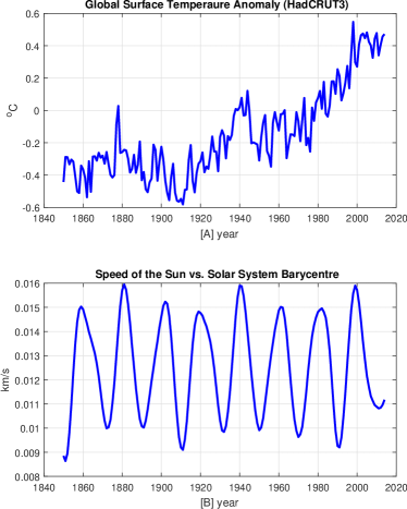
Figure 1: [A] HadCRUT3 global surface temperature (Brohan et al., 2006); [B] Speed of the Sun relative to the barycenter of the solar system. Annual means. (For details: Scafetta, 2014, 2016).

Herein I explain that Scafetta (2016) did not specify any value for such two parameters simply because my analysis did not require them. In fact:
1) Holm confused the MSC-CCA method for its reduced-rank approximation known as the Reduced-Rank CCA (MSC-RRCCA). I will explain how the two techniques are used and how the reduced-rank parameter $p$ should be chosen. The reduced-rank operation was developed to attempt to suppress the noise in order to emphasize the signal (Santamaría and Vía, 2007), but it was unnecessary in Scafetta (2016) since I directly evaluated the 95% significance of the MSC-CCA spectral peaks using the random phase significance model (Traversi et al., 2012). In any case, for the specific analysis presented in Scafetta (2016), MSC-CCA and MSC-RRCCA produce identical results when $p$ is varied within its allowed range. Therefore, Scafetta (2016)’s result could not be ambiguous.
2) Regarding the regularization parameter $\epsilon$ (or $\delta$), it is evident that it was added to the algorithm by Holm himself. In fact, this parameter simply does not exist in the original MSC-CCA/MSC-RRCCA definition or code and, therefore, I could not have used it. Herein I will explain why MSC-CCA/MSC-RRCCA, in most cases, does not require it even when the correlation matrices are singular.

Contrary to Holm’s opinion, his failure to reproduce Scafetta (2016) was not due to any ambiguity present in my work regarding presumed undocumented parameters. Holm just used different analysis algorithms instead of the real MSC-CCA/MSC-RRCCA one. In fact, for his figures 2-4, Holm (2018, section 3, paragraph 2) apparently adopted a MatLab “gcs_cca_1D.m” function (modified with a regularization parameter) that, as people familiar with these codes know, evaluates the Generalized Coherence Spectrum using the Canonical Correlation Analysis (GCS-CCA), proposed only in Ramírez et al. (2008), which Scafetta (2016) did not even cite. For his figure 5, Holm used the basic form of the Welch MSC algorithm (his eq. 3) by erroneously equating it to the non-parametric MSC-CCA (his eq. 11). Thus, Holm (2018) is rather misleading since he always claimed to use the MSC-CCA methodology while, in reality, he adopted different MSC methodologies.

To avoid any possible misinterpretation, I now provide as an electronic supplement the Matlab codes to replicate the MSC-CCA analysis of Scafetta (2016).

2 MSC-CCA and MSC-RRCCA

MSC-CCA and MSC-RRCCA are differently defined. Santamaría and Vía (2007) clearly distinguished between them although the main intent of their work was to develop the parametric MSC-RRCCA algorithm, which is one of the improved versions of MSC-CCA. Zheng et al. (2008) showed that MSC-CCA belongs to a family of non-parametric MSC estimators of the type:

$${}^{\alpha}\gamma_{xy}^{2}(\omega_{L})=\frac{\left|\mathbf{f}_{L}^{H}\mathbf{R}{}_{xx}^{\text{\textminus}\alpha}\mathbf{R}_{xy}\mathbf{R}{}_{yy}^{\text{\textminus}\alpha}\mathbf{f}_{L}\right|^{2}}{(\mathbf{f}_{L}^{H}\mathbf{R}{}_{xx}^{1\text{\textminus}2\alpha}\mathbf{f}_{L})(\mathbf{f}_{L}^{H}\mathbf{R}{}_{yy}^{1\text{\textminus 2}\alpha}\mathbf{f}_{L})},$$ (1)

where $x$ and $y$ are two time series of $N$ data, $\mathbf{R}_{xx}$, $\mathbf{R}_{yy}$ and $\mathbf{R}_{xy}$ are the correlation and cross-correlation matrices, $\mathbf{f}_{L}$ is the Fourier vector, $\mathbf{f}_{L}=\left[1\>e^{jw}\>\ldots\>e^{jw(L-1)}\right]^{T}/\sqrt{L}$, $L$ is the window length parameter, $\omega$ is the frequency, $0\leq{}^{\alpha}\gamma_{xy}^{2}\leq 1$ and $\alpha\in[0,1]$ is the exponential characterizing the estimator. MSC-CCA is defined as:

$$\gamma_{xy}^{2}(\omega,L)=\left|\mathbf{f}_{L}^{H}\mathbf{R}_{xx}^{\text{\textminus}0.5}\mathbf{R}_{xy}\mathbf{R}_{yy}^{\text{\textminus}0.5}\mathbf{f}_{L}\right|^{2},$$ (2)

where $\mathbf{C}_{xy}=\mathbf{R}_{xx}^{\text{\textminus}0.5}\mathbf{R}_{xy}\mathbf{R}_{yy}^{\text{\textminus}0.5}$ is the coherence matrix. The adoption of the square root ($\alpha=0.5$) makes MSC-CCA a midway algorithm between the Welch ($\alpha=0$) and the MVDR ($\alpha=1$) MSC methods which optimizes its MSC performance. In fact, as the parameter $\alpha$ decreases from 1 to 0, the signal mismatch problem reduces at the expense of a decrease in frequency resolution (Zheng et al., 2008). In fact, computer tests demonstrate the MSC-CCA advantages such as a better spectral resolution versus the Welch’s estimator (implemented in the MatLab mscohere function) and the avoidance of the signal canceling problems of the minimum variance distortion-less response (MVDR) estimator (cf.: Santamaría and Vía, 2007; Scafetta, 2016; Zheng et al., 2008).

An optional operation can be added to the MSC-CCA algorithm to filter out the lowest MSC value frequencies, which are interpreted as noise or non-coherent signals. Santamaría and Vía (2007) labeled this methodology Reduced-Rank CCA (MSC-RRCCA). This operation is possible because $\mathbf{C}_{xy}$ can be decomposed by singular value decomposition (SVD) as $\mathbf{C}_{xy}=\mathbf{U}\mathbf{\Lambda}\mathbf{U}^{H}$: where $\mathbf{U}\mathbf{U}^{H}=\mathbf{I}$ , $\mathbf{U}$ contains the singular vectors of $\mathbf{C}_{xy}$ and $\mathbf{\Lambda}$ is a diagonal matrix with non-negative real singular eigenvalues, $k_{i}^{2}$, for $i=1,\ldots,\>L$, sorted in descending order. Thus, it is possible to select a number $p<L$ of eigenvalues considered to be the most significant ones, and substitute the coherence matrix $\mathbf{C}_{xy}$ with its reduced-rank approximation of order $p$: $\tilde{\mathbf{C}}_{xy,p}=\mathbf{U}\tilde{\mathbf{\Lambda}}_{p}\mathbf{U}^{H}$. Santamaría and Vía (2007, figre 4) only proposed a qualitative methodology for the choice of $p$ based on a visual inspection of how the singular eigenvalue function drops: their examples suggests that $p$ could be chosen as $k_{p}^{2}>0.5\geq k_{p+1}^{2}$. More recently, Shao et al. (2014) proposed a generalized likelihood ratio test (GLRT) methodology. In any case, the RR diagonal matrix $\tilde{\mathbf{\Lambda}}_{p}$ is obtained by setting $k_{i}^{2}=0$ for $i=p+1,\ldots,\>L$, and MSC-RRCCA is defined as

$$\tilde{\gamma}_{xy}^{2}(\omega,L,p)=\left|\mathbf{f}_{L}^{H}\tilde{\mathbf{C}}_{xy,p}\mathbf{f}_{L}\right|^{2},$$ (3)

with $0\leq\tilde{\gamma}_{xy}^{2}\leq\gamma_{xy}^{2}\leq 1$ (e.g. Shao et al., 2014). Eqs. 2 and 3 show that MSC-CCA and MSC-RRCCA differ. However, when $p=L$ the latter exactly coincides with the former and, therefore, MSC-RRCCA generalizes MSC-CCA. When $p<L$, MSC-RRCCA is a kind of MSC-CCA filtered off of its less relevant MSC values. However, if the only excludable singular eigenvalues are already equal to zero, which occurs when $\mathbf{C}_{xy}$ is singular, MSC-RRCCA and MSC-CCA produce exactly the same output. This is the case for the analysis performed in Scafetta (2016) where I used a traditional method to directly evaluate the 95% significance of the MSC spectral peaks.

Based on the above definitions it is clear that (Holm, 2018)’s claim that MSC-CCA “assumes a model with a predetermined number of sinusoids for the climate data” is erroneous. In fact, MSC-CCA does not eliminate any singular eigenvalues of the coherence matrix $\mathbf{C}_{xy}$ and, therefore, it does not apply any frequency filtering or selection. Moreover, such a selection does not occur even when MSC-RRCCA is adopted if the excluded singular eigenvalues of $\mathbf{C}_{xy}$ are already all equal to zero.

3 Scafetta (2016) cited and used MSC-CCA

Holm (2018)’s main allegation is that Scafetta (2016) did not specify the “values of key parameters in the CCA method” that, in his opinion, I should have necessarily adopted. The first one would be the reduced-rank parameter $p$ introduced above. Yet, Scafetta (2016) only used MSC-CCA in its basic form as implicit in the fact that I did not explicit any value of $p$. Thus, a reader had to realize that the RR option was not used or that I used it at its default value $p=L$. Evidently, Scafetta had no obligation to explicit the value of a parameter that is either missing in the MSC-CCA algorithm (Eq. 2) or it is automatically set to its default value by the original code itself.

In fact, the Matlab reduced-rank MSC-CCA code provided by its authors, “CCA_MSC.m,” contains also the command “if isempty(R) R=L;” which sets the reduced rank parameter $p$ (labeled $R$) to $L$ when its input is left empty. To avoid any possible confusion or misinterpretation, I now provide as an electronic supplement the Matlab codes to replicate the MSC-CCA analysis of Scafetta (2016). Thus, according to its own authors, MSC-CCA is the default version of MSC-RRCCA, as the mathematical logic of the equations 1 and 2 also imply. On the contrary, Holm’s misunderstanding likely occurred because he used the MatLab “gcs_cca_1D.m” function, written as gcs_cca_1D(x,L,K,P) (see Supplement), that depends explicitly on a reduced-rank parameter “$P$” that must be set to some value.

Moreover, Scafetta (2016) used the adjective “reduced-rank” just in page 2126 when I introduced the content of Santamaría and Vía (2007) that compared several MSC methods, but I never used it when I presented or discussed my own calculations. I was also very careful to title figures 4 and 7 in Scafetta (2016) just as “Canonical Coordinates” and “Canonical Coordinates (CCA)”, respectively, while Santamaría and Vía (2007) titled their figures 1-3 “reduced-rank CCA” since they showed MSC-RRCCA examples while I showed MSC-CCA ones. Note that also Zheng et al. (2008) showed examples of MSC-CCA without any reduced rank.

Despite the numerous evidences that I did not use the RR option, Holm (2018) only exploited a possible minor typo present in page 2126 of Scafetta (2016) to claim that I was ambiguous regarding whether I was using MSC-RRCCA or MSC-CCA. Yet, the typo likely occurred because the original authors labeled their code as “CCA_MSC.m.” This label is ambiguous since the code actually implements MSC-RRCCA while MSC-CCA is interpreted as its default state (see Supplement). Consequently, I likely wrote “CCA–MSC is based on the reduced rank coherence matrix…” because I was implicitly referring to the MatLab code label. However, it is true that the use of the term "reduced-rank" in Scafetta (2016) might have confused a few readers. In any case, Section 5 demonstrates that Holm’s “ambiguity argument” is irrelevant because under the same statistical condition of the analysis proposed in Scafetta (2016), both MSC-CCA and MSC-RRCCA produce an identical result.

4 Holm’s regularization parameter is unnecessary

Holm (2018)’s second claim is that Eq. 2 had to be modified using a regularization parameter $\epsilon$ (or $\delta$), which he supposed that I had used too but I left “undocumented”. His Eq. 9 expressed such a modification as $\mathbf{R}_{xx}=\mathbf{R}_{xx}+\epsilon\mathbf{I}$, which is also improperly written because it would imply $\epsilon=0$, while Holm set $\epsilon\neq 0$. Evidently, Scafetta (2016) did not mention any regularization parameter simply because it does not exist in Eq. 2 nor in Eq. 3. Moreover, it is not mentioned in Santamaría and Vía (2007) nor included in their “CCA_MSC.m” code.

Holm motivated the addition of such a regularization parameter because when he tried his “gcs_cca_1D.m” function on the physical records he found MSC estimates often larger than unity. Holm (2018) interpreted his results by claiming that a regularization parameter would be necessary to avoid “numerical problems due to possible singularity of” the correlation matrices. Yet, Holm’s statements are explicit admissions only that his code was not working properly. Indeed, MSC values cannot be larger than unity, which implies a numerical problem or a mathematical flaw in the algorithm or in the code.

Contrary to Holm’s opinion, I found that adding a regularization parameter to the MSC-CCA algorithm is often unnecessary because most matrix singularity issues are already efficiently handled by MatLab when the code is written as in the Supplement. Essentially, in processing Eq. 2, Matlab often evaluates $\mathbf{R}_{xx}^{-1/2}$ and $\mathbf{R}_{yy}^{-1/2}$ and then it factors their theoretical infinities using the singularities of $\mathbf{R}_{xy}$ as if $\sqrt{\infty}\cdot 0\cdot\sqrt{\infty}=0$, which prevents the NaN error. The same result could be obtained by adding a very small regularization term to the correlation matrices but, as said, in Scafetta (2016) this was unnecessary since Matlab did not give any warnings regarding an encountered numerical failure. In fact, simple tests show that Matlab evaluates $\mathbf{A}^{-0.5}$ even when $\mathbf{A}^{-1}$ fails because the matrix $\mathbf{A}$ is singular. Probably, the computational rounding errors slightly break the matrix singularity and its positive semi-definite status. Then, the square root makes it easier to keep the values within the double floating-point limits of the computer that can handle positive real numbers between $2\cdot 10^{-308}$ and $2\cdot 10^{308}$. This fact makes the MSC-CCA code significantly more stable than, for example, the MVDR estimator (Benesty et al., 2006) whose published code uses a small and fixed regularization parameter (which I did not change) to slightly modify the correlation matrices to permit their numerical inversion in singularity cases.

Moreover, once the coherence matrix $\mathbf{C}_{xy}$ of Eq. 2 is numerically well defined, the RR operation can be applied without any problem. Thus, also Holm (2018)’s claim that the regularization parameter would be “unnecessary” when the RR option is not used, is incorrect. It does not reflect how Eqs. 2 and 3 work, which necessarily imply that $0\leq\tilde{\gamma}_{xy}^{2}\leq\gamma_{xy}^{2}\leq 1$ (Shao et al., 2014), while Holm’s claim would imply that in some cases and for some frequencies $0\leq\gamma_{xy}^{2}\leq 1<\tilde{\gamma}_{xy}^{2}$.

Regarding the GCS-CCA method, Holm’s own tests (figures 2-4) showed that it still did not properly work even after the addition of his regularization parameter. Thus, contrary to Holm’s opinion, the gcs_cca_1D.m function could not be fixed in his proposed manner. Proposing a proper correction of the GCS-CCA method and/or of its code is out of the scope of this work.

5 Step-by-step replication of Scafetta (2016)

The MSC-CCA analysis (Eq. 2) of the physical data is repeated as in Scafetta (2016) using $L=110$ and compared against the MSC-RRCCA one: see Figure 2. There are $N=165$ annual values from 1850 to 2014, the last year when the HadCRUT3 temperature record by Brohan et al. (2006) was provided. I used this record, and not the updated HadCRUT4 version, because both Holm and I have used it since 2010: the results would not change significantly using HadCRUT4. The temperature record is detrended of its quadratic trend as done in Scafetta (2016) before the analysis.

Figure 2A shows the singular eigenvalues $k_{i}^{2}$ for $i=1,\ldots\>,110$ of the coherence matrix $\mathbf{C}_{xy}$ ordered from the larger to the smaller. They are nearly equal to 1 for $i=1,\ldots\>,56$ and nearly equal to zero for $i=57,\ldots\>,110$. Let us make some considerations:

1) The 56 singular eigenvalues larger than zero are expected since the rank of $\mathbf{R}_{xx}$, $\mathbf{R}_{yy}$ and $\mathbf{R}_{xy}$ is $165-110+1=56$ while their size is $110\times 110$: only 56 110-long different moving windows can be made using 165 data.

2) The other $110-56=54$ singular eigenvalues of $\mathbf{C}_{xy}$ are nearly equal to zero. Thus, MatLab efficiently worked around the theoretical singularities of the matrices.

3) Figure 2A also suggests that if MSC-RRCCA is applied, the reduced-rank parameter $p$ could be set only between 56 and 110. In fact, $p$ should not be set below 56 because all singular eigenvalues are nearly equivalent to each other and close to 1, and it would be impossible to discriminate them between the most and the least relevant ones. This consideration would be also consistent with the GLRT-based rank detection method (Shao et al., 2014) since its test variable $2\varsigma_{p}=-N\sum_{i=p+1}^{L}\ln(1-\gamma_{i}^{2})$ would essentially be equal to infinite for $p\leq 56$ and equal to zero for $p\geq 57$. Thus, within the allowed range, the selection of $p$ does not produce any variation in the result because $k_{i}^{2}=0$ for $i=57,\ldots\>,110$.

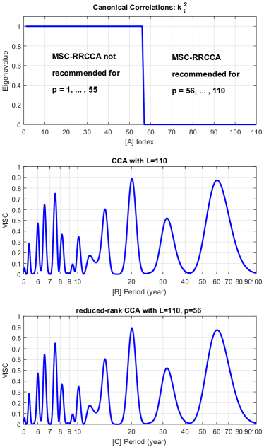
Figure 2: Coherence analysis between reccomended the data shown in Figure 1 using $L=110$. [A] Singular eigenvalues; [B] CCA; [C] Reduced-Rank CCA with $p=56$. Compare with Scafetta (2016).

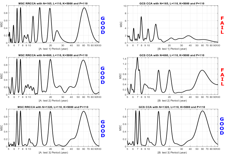
Figure 3: Comparison between MSC-CCA (left) and GCS-CCA (right) with the given parameters using synthetic records as discussed in Section 6. MSC-CCA performs always well and it is stable because the five theoretical coherent periods equal to 6.6, 7.4, 14, 20 and 60 year are always found. On the contrary, GCS-CCA performs well only in test #3. Note the severe failure of GCS-CCA in test #1 and test #2 since values with $MSC>1$ are observed.

Figures 2B and 2C show that MSC-CCA and MSC-RRCCA with $p=56$ produce exactly the same result. Both analyses show very strong coherence peaks at 20- and 60-year periods ($MSC\approx 0.9$) and reproduce exactly Scafetta (2016, figure 4D and 7).

The result is confirmed also using the monthly record as in Holm (2018) (Scafetta (2016) used the annual one) and using a coherence window $L=(N+1)/2=83$ (see also Section 8): in the latter case the matrices $\mathbf{R}_{xx}$, $\mathbf{R}_{yy}$ and $\mathbf{R}_{xy}$ are not singular and, therefore, there are no numerical issues. The Supplement also includes the original “CCA_MSC.m” code to reproduce Santamaría and Vía (2007) to assure readers that I am using the right algorithm. Moreover, the reliability of my MatLab codes is further confirmed by a simple computer experiment simulating the same statistical constrains of the physical data analyzed in Scafetta (2016): see also Figure 3.

In conclusion, contrary to Holm (2018)’s claims, Scafetta (2016) cannot be ambiguous because (1) the regularization parameter $\delta$ was not required and (2) both MSC-CCA and MSC-RRCCA produce the same output. A reader simply had to use the indicated analysis techniques (MSC-CCA or MSC-RRCCA would have been equivalent) and to do it properly, but Holm used different algorithms. Then, Scafetta (2016, figure 7) directly evaluated the significance of the MSC-CCA results using Monte Carlo simulations based on the random phase model: see also Section 8.

6 MSC-CCA versus GCS-CCA

Ramírez et al. (2008) apparently considered the GCS-CCA as a multi-sequence extension of MSC-CCA, which processes just two sequences (Santamaría and Vía, 2007). However, I will herein demonstrate that this is not the case. The two codes can generate significantly different results under specific statistical conditions, which explains the alternative conclusions in Scafetta (2016) and Holm (2018). In fact, the “gcs_cca_1D.m” function was not written in such a way to naturally implement the MSC-CCA algorithm in a 2-signal case because the two functions handle the data differently. For example, for two records GCS-CCA uses 2Lx2L coherence matrices while MSC-CCA uses LxL coherence matrices.

Since Holm (2018) found that the gcs_cca_1D.m function was unreliable using specific physical data while in Ramírez et al. (2008) it was working well using generic synthetic examples, it is necessary to test whether and under which specific statistical circumstances GCS-CCA and MSC-CCA give different results. I will do this now by comparing simple computer tests where the same pair of synthetic records are processed with both techniques. I used the gcs_cca_1D.m function that the authors sent me in 2014, which replicates Ramírez et al. (2008) (see Supplement). However, this function might not coincide with that used in Holm (2018) because (1) Holm did not published it and (2) he stated that, since it was not working, he and/or Ramírez altered it with a regularization parameter $\delta$. The exact nature of the code modifications were not provided in Holm (2018) so that also his figures 2-4 cannot be replicated. Therefore, my results might appear different from those that Holm could get with his code, but they show what the original gcs_cca_1D.m function by Ramírez et al. (2008) really does.

Pairs of synthetic records were generated with five harmonics with periods equal to 6.6, 7.4, 14, 20 and 60 year, as similarly found in the physical data discussed in Scafetta (2016), plus Gaussian noise: see the Supplement for details. I use $L=110$, $K=5000$ equispaced frequencies and $P=L=110$, which means that the reduced-rank option was not used. However, I progressively increase the length of the record as $N_{1}=165$ (as in the original physical records), $N_{2}=4*165$ and $N_{3}=8*165$.

Figure 3 depicts the results. MSC-CCA works always well in all three tests, it is stable and always finds the expected 5 coherent harmonics, which are characterized by $0.9<MSC<1$. On the contrary, GCS-CCA works well only when N is very large relative to $L$ (test #3) but, as $N$ decreases, it becomes progressively more and more unstable and completely fails for $N=165$ where the “estimate of MSC often became much higher than unity”, as Holm (2018) stated to have found in his tests. By running again and again the same code, only the GCS-CCA result depicted in test #3 remains stable, while the result depicted in test #1 changes greatly at each run and always fails while that of test #2 fails in some case.

Thus, MSC-CCA and GCS-CCA perform similarly only when $N\gg L$. In these simulations, GCS-CCA works well when $N\geq 5L$. However, for the specific analysis presented in Scafetta (2016), which required investigating the low-frequency spectrum and used $L=110$ and $N=165$, GCS-CCA fails. In conclusion, since GCS-CCA statistically collapses when it attempts to reproduce Scafetta (2016), using GCS-CCA instead of MSC-CCA definitely explains Holm’s inability to reproduce my result.

7 Holm (2018)’s figure 5 is misleading

Regarding his figure 5, Holm (2018) claimed to be using MSC-CCA with $\delta=0$ and $P=L$ (as Scafetta (2016) could have done), but I found that his result was not reproducible even when the original gcs_cca_1D.m function was used. His figure 5 shows MSC values between 0 and 1, but I found much-higher-than-unity MSC values: see Figure 4. I used monthly records as in Holm (2018), but a similar failure occurs using the yearly record. Indeed, the result depicted in Holm’s figure 5 shows contradictions by his own acknowledgment (see his Section 2) that using the original algorithm “the estimate of MSC often became much higher than unity.” This was the reason why Holm added the regularization parameter $\delta$ to the algorithm. He also observed that for high value of $p$ (note that $p=L$ is its maximum value) $\delta$ was necessary and had to be high since, if it was set too low (note that $\delta=0$ is its lowest value), his algorithm gave $MSC>1$ (cf. his figure 2 and related comments). Thus, the severe numerical instability disclosed by Holm is perfectly consistent with my analysis, but not with the result shown in his figure 5.

Indeed, Holm’s figure 5 was apparently not obtained by setting $\delta=0$ and $P=L$ in the same code used for his figures 2-4. Holm stated that he used his eq. 3 that, however, is the Welch’s averaged periodogram method implemented in the MatLab “mscohere” function and can be obtained also from Eq. 1 with $\alpha=0$. Holm (2018) justified such a choice by claiming that his eq. 3 represented MSC-CCA without rank reduction (his eq. 11), which is erroneous (cf. Section 2 and Zheng et al., 2008).

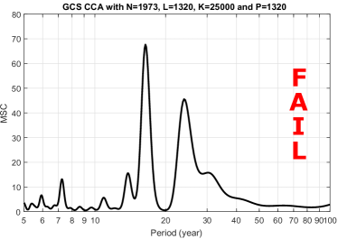
Figure 4: GCS-CCA analysis (with the original “gcs_cca_1D.m” function) of the physical records (monthly resolution) without the RR filtering ($P=L$). Note the severe algorithm failure ($MSC>1$).

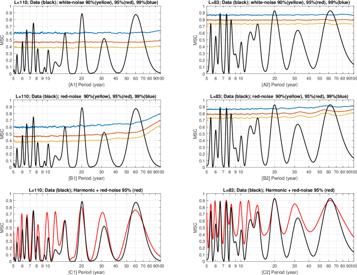
Figure 5: MSC-CCA between the global surface temperature record and the Sun’s speed against different significance models as explained in Section 8. The coherence frequency peaks at 20- and 60-year periods pass well the 95% level in all cases.

8 The 95% significance problem

Holm (2018, figure 5) also questioned that the spectral coherence at the 20- and 60-year periods was 95% significant. However, in Scafetta (2016, figure 7) their 95% significance is well met. Holm and I presumably used the same random phase significance model (cf.: Traversi et al., 2012) but, as proven above, we did not use the same MSC algorithm and Scafetta (2016) already proved that the Welch MSC algorithm, which was used by Holm instead of MSC-CCA, provides uncertain results. Moreover, there is some issue regarding the appropriate significance model to be used. For example, the wavelet transform coherence (WTC) proposed by Grinsted et al. (2004), where AR(1) significance models are assumed by default, shows that in the critical 17-22 year and around the 60-year range the spectral coherence is large enough to pass well the 95% significance level. However, Holm (2015, figure 5) claimed a different result using the random phase significance model, which assumes that one record is nearly harmonic: in this case the problem could have be induced by the WTC low spectral resolution yielding Scafetta (2016) to propose the adoption of the MSC-CCA high resolution method. Thus, the important role of the significance model needs to be now clarified.

The basic assumption is that two records are of the type: $x(t)=signal(t)+noise(t)$. The issue is to determine how likely the observed MSC spectral peaks could be artifacts of the noise function. Using Monte Carlo method simulations, it is possible to determine the MSC-CCA significance curves that various forms of noise models could produce. Note that the direct adoption of the confidence methodology voids the necessity of using the RR operation. There are three basic cases:
1) White-noise vs. white-noise. It is assumed that the two records are affected just by random white noise. The test is performed by generating 10000 pairs of Gaussian noise sequences with N=165 and their MSC-CCA curves are evaluated. Then, for each frequency, I took the 90%, 95% and 99% top values among the 10000 estimates.
2) Red-noise vs. red-noise. It is assumed that both records are AR(1) processes. The test is performed by generating 10000 pairs of AR(1) sequences calibrated on the data records with N=165 and evaluate their MSC-CCA curves. The AR(1) records are obtained with the model $x_{n}=\alpha x_{n-1}+\xi_{n}$ for $n=1,2,\ldots,\,N$, where $\xi_{n}$ is a sequence of Gaussian random noise and the AR(1) parameter $\alpha$ is measured on the physical data record. I got $\alpha=0.94$ for the astronomical record once detrended of its mean and $\alpha=0.58$ for the temperature record once detrended of a parabolic trend. Then, I did as above.
3) Harmonic signal vs. red-noise. One record is assumed harmonic while the other (e.g. the temperature record) is an AR(1) process. This case is interesting because a nearly harmonic record (e.g. the astronomical one) would a-priory select specific harmonics that could give origin to high specific MSC peaks even if tested against just noise. The test is performed by pairing the astronomical record with 10000 AR(1) sequences modeling the temperature record as above. Then, for each frequency, I took the 95% top value among the 10000 estimates.

Figure 5 shows the evaluated significance curves against the measured MSC-CCA curves generated by the physical records using $L=110$ and $L=83$. The noise models #1 and #2 give a 99% significance for many MSC peaks including those at 20- and 60-year periods. Test #3 shows results similar to those found in Scafetta (2016, figure 7) using the random phase significance model, which the method approximately simulates, and give a very safe 95% significance level for the same coherence spectral peaks. Thus, the 6 panels of Figure 4 fully confirm Scafetta (2016) and my previous studies, and contradict the contrary claims made in Holm (2014, 2015, 2018).

Regarding test #3, I note that if one of the two records is already known to be harmonic (e.g. orbital astronomical records, cf.: Scafetta, 2014, figure 5) and its main harmonics are already known, using spectral coherence methodologies should be unnecessary in most cases. In fact, in such situations the spectral coherence is logically reduced to the simple verification of whether the second record (e.g. the temperature one) is characterized by spectral frequencies consistent with those already known to exist in the harmonic signal. Spectral analysis confirms with a 99% significance the presence of quasi 20- and 60-year harmonics in the global surface temperature: this was the original logic followed in Scafetta (2010, figures 3, 6 and 9) and in Scafetta (2016, figure 2B).

9 Conclusion

I have demonstrated that Holm (2018) failed to reproduce Scafetta (2016) not because I left two parameters, $\delta$ and $p$, “undocumented”, as he claimed, but because he mistook the MSC-CCA method (Santamaría and Vía, 2007), which is what Scafetta (2016) used and referenced, for two different MSC methodologies. For his figures 2-4, Holm apparently adopted the GCS-CCA methodology proposed in Ramírez et al. (2008) altered with a regularization term without realizing that it implemented a different algorithm. Herein I showed (1) that the MSC-CCA methodology did not need the two parameters proposed by Holm and (2) that the “gcs_cca_1D.m” function, which Holm adopted, becomes progressively unstable and collapses under the specific statistical conditions required to replicate Scafetta (2016). Of course, Scafetta (2016) was not responsible about Ramírez et al. (2008), the “gcs_cca_1D.m” function and Holm adopting it to try to reproduce my results because I always cited and used only the reliable MSC-CCA code sent me by Vía. For his figure 5, Holm was supposed to use MSC-CCA with $\delta=0$ and $P=L$ and mentioned that he still could not replicate my results. Yet, for this figure he used his eq. 3, representing the basic Welch MSC algorithm (Eq. 1 with $\alpha=0$) by erroneously equating it to the non-parametric MSC-CCA algorithm (Eq. 1 with $\alpha=0.5$).

Moreover, no formal ambiguity could exist in Scafetta (2016) regarding the adoption of the RR parameter $p$, as Holm also charged, because in the specific case both MSC-CCA and MSC-RRCCA produce the exact same result when properly used. Moreover, the RR option was not needed in Scafetta (2016) because I adopted Monte Carlo simulations based on the random phase model to evaluate the 95% statistical significance of MSC spectral peaks. Thus, the “noise” present in the MSR-CCA result did not need to be suppressed with a RR filtering. Finally, contrary to Holm (2018)’s claims, I have further confirmed the spectral coherence with at least a 95% significance at the 20- and 60-year periods between the analyzed climatic and astronomical records using various standard noise models.

Holm (2018) made secondary comments referring also to his past critiques (Holm, 2014, 2015) to my previous studies, for example in his Section 4.3. Interested readers can find my past rebuttals in Scafetta (2014, 2016). A latest general review on the topic of an astronomical origin of climate oscillations throughout the Holocene is found in Scafetta et al. (2016) and in its references.

The online Supplement provides data and Matlab codes necessary to reproduce all results shown above, the original “CCA_MSC.m” and “gcs_cca_1D.m” codes and a code to reproduce Holm’s figure 5 using the mscohere function. See: https://doi.org/10.1016/j.asr.2018.05.014

References

- Benesty et al. (2006) Benesty, J., Chen, J., Huang, Y. 2006. Estimation of the coherence function with the MVDR approach. 2006 IEEE Int. Conf. Acoust. and Speech Sign. Proc., 3, 500–503.
- Brohan et al. (2006) Brohan, P., Kennedy, J.J., Harris, I., Tett, S.F.B., Jones, P.D., 2006. Uncertainty estimates in regional and global observed temperature changes: a new dataset from 1850. J. Geophys. Res., 111, D12106.
- Grinsted et al. (2004) Grinsted, A., Moore, J. C., Jevrejeva, S., 2004. Application of the cross wavelet transform and wavelet coherence to geophysical time series. Nonlinear Proc. Geophys., 11, 561–566.
- Holm (2014) Holm, S., 2014. On the alleged coherence between the global temperature and the sun’smovement. J. Atmos. Solar-Terrestr. Phys., 110–111, 23–27.
- Holm (2015) Holm, S., 2015. Prudence in estimating coherence between planetary, solar and climate oscillations. Astrophys. Space Sci., 357, 1–8.
- Holm (2018) Holm, S., 2018. Comment on “High resolution coherence analysis between planetary and climate oscillations”. Advances in Space Research. https://doi.org/10.1016/j.asr.2017.09.034
- Ramírez et al. (2008) Ramírez, D., Vía, J., Santamaría, I., 2008. A generalization of the magnitude squared coherence spectrum for more than two signals: definition, properties and estimation. 2008 IEEE Int. Conf. Acoust. and Speech Sign. Proc., 3769–3772.
- Santamaría and Vía (2007) Santamaría, I., Vía, J., 2007. Estimation of the magnitude squared coherence spectrum based on reduced- rank canonical coordinates. 2007 IEEE Int. Conf. Acoust. and Speech Sign. Proc., 3, 985–988.
- Scafetta (2010) Scafetta, N., 2010. Empirical evidence for a celestial origin of the climate oscillations and its implications. J. Atmos. Sol. Terr. Phys., 72, 951–970.
- Scafetta (2014) Scafetta, N., 2014. Discussion on the spectral coherence between planetary, solar and climate oscillations: a reply to some critiques. Astrophys. Space Sci. 354, 275–299.
- Scafetta (2016) Scafetta, N., 2016. High resolution coherence analysis between planetary and climate oscillations. Advances in Space Research, 57, 2121–2135.
- Scafetta et al. (2016) Scafetta, N., Milani, F., Bianchini, A., Ortolani, S., 2016. On the astronomical origin of the Hallstatt oscillation found in radiocarbon and climate records throughout the Holocene. Earth-Science Reviews, 162, 24–43.
- Shao et al. (2014) Shao, Q., Peng, R., Zheng, C., 2014. Estimation of a generalized non-parametric magnitude squared coherence spectrum using the GLRT-based rank detection. In IEEE Inter. Conf. on Signal Process. (ICSP), 189-193.
- Traversi et al. (2012) Traversi, R., Usoskin, I., Solanki, S., Becagli, S., Frezzotti, M., Severi, M., Stenni, B., Udisti, R., 2012. Nitrate in polar ice: a new tracer of solar variability. Sol. Phys., 280, 237–254.
- Zheng et al. (2008) Zheng, C., Zhou, M., Li, X., 2008. On the relationship of non-parametric methods for coherence function estimation. Signal Process., 88, 2863–2867.