Two- and three-body interactions in $\varphi^{4}$ theory from lattice simulations

Abstract

We calculate the one-, two- and three-particle energy levels for different lattice volumes in the complex $\varphi^{4}$ theory on the lattice. We argue that the exponentially suppressed finite-volume corrections for the two- and three-particle energy shifts can be reduced significantly by using the single particle mass, which includes the finite-size effects. We show numerically that, for a set of bare parameters, corresponding to the weak repulsive interaction, one can reliably extract the two- and three-particle energy shifts. From those, we extract the scattering length, the effective range and the effective three-body coupling. We show that the parameters, extracted from the two- and three-particle energy shifts, are consistent. Moreover, the effective three-body coupling is significantly different from zero.

I Introduction

In the last decade, the use of the (multi-channel) Lüscher equation Luescher-torus ; Rummukainen ; Lage-KN ; Lage-scalar ; He ; Sharpe ; Briceno-multi ; Liu ; PengGuo-multi ; Morningstar:2017spu has become a standard tool for the extraction of the infinite-volume two-particle scattering phase shifts and inelasticities from the energy spectrum on the lattice Helmes:2017smr ; Liu:2016cba ; Helmes:2015gla ; Romero-Lopez:2018zyy ; Wilson-pieta ; Bolton:2015psa ; Briceno:2016mjc ; Briceno:2017qmb ; Guo:2018zss . Further, the Lellouch-Lüscher formalism, as well as its generalizations to the case of the coupled two-particle channels, have been successfully used for the measurement of various matrix elements with two-particle final states, as well as for the calculation of the resonance form factors Lellouch:2000pv ; Hansen:2012tf ; Briceno:2014uqa ; Briceno:2015csa ; Bernard:2012bi ; Agadjanov:2014kha ; B-decays ; Briceno:2016kkp . Very recently, the focus in the development of the formalism has been shifted from two- to three-particle systems, where a significant amount of work has been done in the course of last few years Polejaeva:2012ut ; Meissner:2014dea ; Guo:2016fgl ; Guo:2017ism ; Briceno:2012rv ; Hansen:2014eka ; Hansen:2015zga ; Hansen:2015zta ; Hansen:2016fzj ; Hansen:2016ync ; Briceno:2017tce ; Kreuzer:2010ti ; Kreuzer:2009jp ; Kreuzer:2008bi ; Kreuzer:2012sr ; Sharpe-recent ; pang1 ; pang2 ; Meng:2017jgx ; Doring:2018xxx ; Mai:2017bge ; Briceno:2018mlh . In particular, the formalism of Refs. pang1 ; pang2 ; Doring:2018xxx provides a systematic fit strategy to the data, even if the latter consists of only few data points with sizable errors (a conceptually similar approach was proposed in Ref. Mai:2017bge ). The output of this fit determines the low-energy constants in the three-particle sector (three-particle force), which can be further used, as an input, in the infinite-volume scattering equations, in order to determine all $S$-matrix elements in the three-particle sector. It is not immediately clear, however, whether this ambitious program can be realized in practice or, in other words, whether the three-body force can be reliably extracted from the lattice data. The present study intends to explore this gap and test the viability of the theoretical framework.

The strategy laid out in Refs. pang1 ; pang2 ; Doring:2018xxx could be briefly summarized as follows: the interactions in the effective Lagrangian, describing three particles, are parameterized by two sets of couplings. The first set of couplings describes the low-energy interactions in the two-particle sub-systems. These can be related to the usual effective range expansion parameters: the scattering length $a$, the effective range $r$, and so on. The second set corresponds to the tower of the three-body local couplings, which are multiplying the operators with an increasing number of space derivatives acting on the fields. At lowest order, there is just a single constant describing the contact non-derivative interaction of three particles at one point. If the particle-dimer picture is used, these two sets of couplings are uniquely translated into the sets describing the dimer-two-particle vertex and the contact particle-dimer interactions. The details are given in Refs. pang1 ; pang2 .

Next, note that the couplings in the two-body sector can be independently fitted to the two-particle phase shift, extracted from the lattice data by using the Lüscher method. On the contrary, the finite-volume spectrum in the three-particle sector, which is determined by the quantization condition derived in Ref. pang2 , depends on both sets of couplings, with the former already fixed from the fit to the two-particle scattering data. Thus, the fit to the three-particle energy levels allows one to determine the first few couplings in the three-particle (particle-dimer) sector. Using the values of the couplings, determined in this way, one may then calculate all infinite volume $S$-matrix elements.

Note also that the presence of the three-body force in the equations (both in infinite and finite volume) is crucial. These equations contain the UV cutoff and, without the three-body force, one could not ensure UV cutoff-independence of the observable quantities, obtained by solving the equations. Namely, the coupling constants should show the log-periodic dependence on the cutoff (see, e.g., Bedaque:1998kg ; Bedaque:1998km ).

The aim of our investigation is, in particular, to answer to the following questions:

• Is the theoretical approach, proposed in Refs. pang1 ; pang2 ; Doring:2018xxx , practically viable? Could one unambiguously extract the effect from the genuinely three-body (particle-dimer) coupling(s) from data with the present computational ressources?

• What is the best fit strategy? At which volumes should the data be taken to be most sensitive to the three-particle coupling(s)?

• Does one have all finite-volume artifacts under sufficient control in order to extract the three-body coupling(s) with a reasonable systematic error?

In order to answer these questions we have used our framework from the beginning to the end to analyze the data in the toy model described by the $\varphi^{4}$ Lagrangian . On the one hand, this model is chosen for the illustration of the fact that the three-body calculations can be systematically carried out even without committing extraordinary computational capabilities. On the other hand, we use this model as an example to discuss the general issues, which were outlined above.

For simplicity, we will from now on assume that the three-particle force is described by the single non-derivative coupling. It will be seen, a posteriori, that the accuracy of lattice data is not yet sufficient for extracting higher-order couplings as well.

It is important to realize that the role of the three-body force in the following situations is physically very different:

• There exists a three-particle bound state: in nature this scenario is realized e.g. in a particular three-nucleon systems (triton). In this case, one can directly extract the pertinent three-body coupling by extrapolating the measured bound-state energy to infinite volume.

• There is no three-particle bound state: in nature this corresponds to e.g. the final-state interactions in the $K\to 3\pi$ decay. In large volumes, the free three-particle energy levels are displaced (such a case was considered, e.g., in Refs. Huang ; Wu ; Tan ; Beane ; Hansen:2015zta ; Hansen:2016fzj ; Sharpe-recent ). The displacement contains the three-particle coupling only at N³LO in the perturbative expansion in $1/L$, where $L$ is the size of the box and, hence, it is legitimate to ask, whether this coupling can be extracted from data at any precision. Further, making $L$ smaller in order to enhance the relative contribution of the three-particle force, one is necessarily confronted with the question about the exponentially suppressed finite volume effects. Does one control these effects to a sufficient precision, to ensure a clean extraction of the three-particle coupling?

We stress here once more that in nature one encounters both scenarios, so it is useful to address them both in the model study. Whereas the extraction of the three-particle coupling in scenario i) is relatively straightforward, the scenario ii) should be given more scrutiny.

In particular, we would like to point out the issue of consistency of the infinite-volume and the finite-volume descriptions of the same system in the framework we are considering. Suppose that scenario ii) is realized. Then, the three-body coupling appears only at order $L^{-6}$ in the perturbative expansion of the ground-state energy level, which starts at $O(L^{-3})$ (to be more precise, a certain cutoff-independent combination of this coupling and the UV cutoff should appear in the expression of the finite-volume energy). Owing to this fact, the extracted value of this coupling will potentially have large errors. This could lead to problems, if the same coupling would emerge at the leading order in the infinite-volume scattering amplitude. It can be seen, however, that this is not the case – the pertinent contribution to the scattering amplitude is suppressed in perturbation theory.

Finally, note that the quantization condition given in Ref. pang2 determines the energy levels implicitly as the solutions of the secular equation. Perturbative expansion in the vicinity of the unperturbed energy levels (both for the ground state and the excited states) is possible JWu . As expected, after this expansion, the results of Refs. Huang ; Wu ; Tan ; Beane ; Hansen:2015zta ; Hansen:2016fzj ; Sharpe-recent for the ground state are reproduced – there is nothing more about the quantization condition in this case. Therefore, in order to fit the three-particle energy levels, we shall further use the expressions given in Ref. Sharpe-recent . A detailed comparison of the threshold expansion given in Ref. Sharpe-recent and the expansion emerging in our approach, es well at the explicit result for the first excited three-particle state is forthcoming JWu .

II Description of the Model

We now turn to the description of the model which will be used in numerical lattice simulations. We choose the complex $\varphi^{4}$ theory, because the charge quantum number protects the mixing of one-, two- and three-particle states. The continuum Euclidean Lagrangian reads

$$\mathcal{L}_{E}=\partial_{\mu}\varphi_{c}^{\dagger}\partial_{\mu}\varphi_{c}+m^{2}_{0}|\varphi_{c}|^{2}+\lambda_{c}|\varphi_{c}|^{4},$$ (1)

and the discretization is performed as follows:

$$\partial_{\mu}\varphi_{c} \rightarrow(\varphi_{c}(x+a\mu)-\varphi_{c}(x))/a\,,$$ (2)

$$\int d^{4}x \rightarrow a^{4}\sum_{x},$$ (3)

$$a\varphi_{c}(x) \rightarrow\sqrt{\kappa}\varphi_{x}\,,$$ (4)

and this way, the discretized action reads

$$S=\sum_{x} \Big{(}-\kappa\sum_{\mu}(\varphi_{x}^{*}\varphi_{x+\mu}+cc)+\lambda(|\varphi_{x}|^{2}-1)^{2}+|\varphi_{x}|^{2}\Big{)}\,,$$ (5)

with

$$\lambda_{c}=\frac{\lambda}{\kappa^{2}},\quad(am_{0})^{2}=\frac{1-2\lambda-8\kappa}{\kappa}\,.$$ (6)

The interpolating operators used for the one-, two- and three-particle states are:

$$\hat{\mathcal{O}}_{\varphi}(\mathbf{x},t)=\varphi(\mathbf{x},t)\,,~{}\hat{\mathcal{O}}_{2\varphi}(\mathbf{x},\mathbf{y},t)=\varphi(\mathbf{x},t)\varphi(\mathbf{y},t)\,,~{}\hat{\mathcal{O}}_{3\varphi}(\mathbf{x},\mathbf{y},\mathbf{z},t)=\varphi(\mathbf{x},t)\varphi(\mathbf{y},t)\varphi(\mathbf{z},t)\,,$$ (7)

respectively. In principle, one must substract the vacuum expectation value (vev) to an operator before constructing the correlation function. However, the transformation

$$\varphi(\mathbf{x},t)\rightarrow\varphi(\mathbf{x},t)e^{i\pi/n},$$ (8)

is a symmetry of the action and the operators in Eq. 7 have a vanishing vev:

$$\braket{\hat{\mathcal{O}}_{n}(\mathbf{x},t)}=\braket{\varphi(\mathbf{x},t)^{n}}\rightarrow-\braket{\varphi(\mathbf{x},t)^{n}}=0.$$ (9)

This way, the correlation functions for the one-particle state are built as follows:

$$C_{1}(t)=\sum_{t^{\prime}}\sum_{x,y}\braket{\hat{\mathcal{O}}_{\varphi}(\mathbf{x},t^{\prime})\hat{\mathcal{O}}^{\dagger}_{\varphi}(\mathbf{y},t+t^{\prime})}\,,$$ (10)

and, similarly, for the two- and three-particle states. That is, we extract the one-, two- and three-particle energies in the center-of-mass (CM) frame.

The energies can be calculated by fitting the correlation functions to their theoretical form, which can be determined by using the Transfer Matrix formalism:

$$C_{i}(t)=\text{Tr }(e^{-\hat{H}(T-t)}\hat{\mathcal{O}}_{i}(0)e^{-\hat{H}t}\hat{\mathcal{O}}_{i}^{\dagger}(0))/\mathcal{Z}\,,\quad\quad\hat{\mathcal{O}}_{i}=\hat{\mathcal{O}}_{\varphi}\,,\,\hat{\mathcal{O}}_{2\varphi}\,,\,\hat{\mathcal{O}}_{3\varphi}\,,$$ (11)

and calculating explicitly in terms of all possible states:

$$\begin{split}C_{i}(t)&=\sum_{n,m}|\braket{n}{\hat{\mathcal{O}}_{i}}{m}|^{2}e^{-E_{n}(T-t)}e^{-E_{m}t}/\mathcal{Z}\\ &=\sum_{n,m}|\braket{n}{\hat{\mathcal{O}}_{i}}{m}|^{2}e^{-(E_{m}+E_{n})T/2}\cosh((E_{m}-E_{n})(t-T/2))/\mathcal{Z}.\end{split}$$ (12)

This way, the different correlation functions look like:

$$C_{1}(t) =|A_{1}|^{2}e^{-M\frac{T}{2}}\cosh{M(t-T/2)},$$ (13)

$$C_{2}(t) =|A_{2}|^{2}e^{-E_{2}\frac{T}{2}}\cosh{E_{2}(t-T/2)}+|A_{1\to 1}|^{2}e^{-MT},$$ (14)

$$C_{3}(t) =|A_{3}|^{2}e^{-E_{3}\frac{T}{2}}\cosh{E_{3}(t-T/2)}+|A_{1\to 2}|^{2}e^{-(E_{2}+M)\frac{T}{2}}\cosh{(E_{2}-M)(t-T/2)}\,.$$ (15)

The additional terms in $C_{2}$ and $C_{3}$ come from thermal pollution, i.e., antiparticles propagating backwards in time and crossing the periodic temporal boundary. They are relevant, since the matrix elements $A_{1\to 1}\propto\braket{\varphi^{\dagger}}{\hat{\mathcal{O}}_{2\varphi}}{\varphi}$ and $A_{1\to 2}\propto\braket{\varphi^{\dagger}}{\hat{\mathcal{O}}_{3\varphi}}{\varphi\varphi}$ are different from zero and, in general, they are of the same order of magnitude as $A_{2}$ and $A_{3}$, respectively. In contrast to $C_{2}$, the pollution term in $C_{3}$ is time-dependent. Both of these additional terms vanish in the limit of $T\to\infty$ but, for finite $T$, they have to be taken into account in the analysis. For $C_{2}$, this can be done by using the discrete derivative of the correlation function, the so-called shifted correlation function:

$$\tilde{C}_{2}(t)=C_{2}(t)-C_{2}(t+1)\,.$$ (16)

This has also advantage in terms of less correlation among the different time slices Ottnad:2017bjt . Using Eq. (16) turns the functional dependence on $t$ in $C_{2}(t)$ into $\sinh$. For $C_{3}$, we take the time-dependent pollution into account explicitly in our fitting. In doing so, we are using the single particle mass $M$ and the two particle energy $E_{2}$ as an input, determined from $C_{1}$ and $C_{2}$, respectively.

Our ensembles are generated using the Metropolis algorithm with simultaneous updates in the even and odd parts of the lattice. We choose $m^{2}_{0}=-4.9$ and $\lambda_{c}=10.0$ implying $\lambda=0.253308$ and $\kappa=0.159156$. We calculate the spectra in 15 different volumes, $L=[5,18]$ and $L=20$ with $T=24$ and two volumes $L=14,\ 24$ with $T=48$. The number of independent configurations is always in the range 7500-100000 and the errors are calculated through jackknife resampling. A summary of all ensembles can be found in Table 2. For the reasons given in the previous paragraph, we fit the corresponding $\sinh$ functional form to our data for the correlation functions $\tilde{C}_{1}$, $\tilde{C}_{2}$ and $\tilde{C}_{3}$. The excited states are expected to be strongly suppressed because we use charged operators and because of the small value of the renormalized coupling $\lambda_{c}$. In practice, there seems to be no sign of excited states in the correlation functions, and thus the fits are performed to all time slices. This can be seen in the effective mass ($m_{\mathrm{eff}}$) plots compiled in Appendix B, where $m_{\mathrm{eff}}$ is defined through:

$$\frac{\tilde{C}_{1}(t+1)}{\tilde{C}_{1}(t)}=\frac{\sinh(m_{\mathrm{eff}}(t+1-\frac{T}{2}))}{\sinh(m_{\mathrm{eff}}(t-\frac{T}{2}))}\,.$$ (17)

For $C_{2}$, the relation looks identical. For $C_{3}$, the functional form is more complicated, but $m_{\mathrm{eff}}$ can be defined likewise.

III The spectrum in finite volume

In the $\varphi^{4}$ theory in the symmetric phase, which is studied in the present paper, the vertices with the odd number of the field $\varphi$ are barred. This situation resembles the one in chiral perturbation theory (ChPT) and we can straightforwardly use the perturbative expression, obtained in Ref. GL (see also Ref. Colangelo ), to describe the volume-dependence of the single-particle mass. This expression has the following form

$$M_{L}-M=\mbox{const}\,\frac{K_{1}(ML)}{ML}\,,$$ (18)

where $M=M_{\infty}$ and $K_{1}(z)$ denotes the modified Bessel function of first kind. Taking into account the asymptotic expression of the Bessel function for a large value of the argument, we get

$$M_{L}-M=\mbox{const}\,\frac{\exp(-ML)}{(ML)^{3/2}}\,.$$ (19)

The threshold expansion of the two- and three-particle energies can be taken from the literature. For convenience, we generally stick to the notations used Ref. Sharpe-recent (we use lattice units in the formulae below). The two-body energy shift $\Delta E_{2}$ reads:

$$\Delta E_{2}=\frac{4\pi a}{ML^{3}}\,\biggl{\{}1+c_{1}\biggl{(}\frac{a}{\pi L}\biggr{)}+c_{2}\biggl{(}\frac{a}{\pi L}\biggr{)}^{2}+c_{3}\biggl{(}\frac{a}{\pi L}\biggr{)}^{3}+\frac{2\pi ra^{2}}{L^{3}}-\frac{\pi a}{M^{2}L^{3}}\biggr{\}}+O(L^{-7})\,,$$ (20)

where $a$ and $r$ denote the two-body scattering length and the effective radius, respectively, and $c_{1},c_{2},c_{3}$ are known numerical constants. The last term is the relativistic correction, which vanishes at $M\to\infty$.

The three-body energy shift of the ground-state level $\Delta E_{3}$ takes the form:

$$\begin{split}\Delta E_{3}=&\frac{12\pi a}{ML^{3}}\biggl{\{}1+d_{1}\biggl{(}\frac{a}{\pi L}\biggr{)}+d_{2}\left(\frac{a}{\pi L}\right)^{2}+\frac{3\pi a}{M^{2}L^{3}}+\frac{6\pi ra^{2}}{L^{3}}\\ &+\left(\frac{a}{\pi L}\right)^{3}d_{3}\log\frac{ML}{2\pi}\biggr{\}}-\frac{D}{48M^{3}L^{6}}+O(L^{-7})\,,\end{split}$$ (21)

where $d_{1},d_{2},d_{3}$ are the known numerical constants and the parameter $D$ is a sum of different terms including the three-body coupling constant we are looking for (or, the divergence-free three-body scattering amplitude ${\cal M}_{3,thr}$ in the notations of Ref. Sharpe-recent ). The individual terms in this sum (including the three-body coupling) depend on the ultraviolet cutoff – only the sum of all terms in $D$ is cutoff-independent. In addition, the quantity $D$ depends on the choice of the scale in the logarithm, which is present in Eq. (21) – there, it is chosen to be equal to $M$, which is the only available natural scale in the theory. Choosing any other scale around this natural scale leads to an additive contribution to $D$. Consequently, our goal can be re-formulated as follows: we want to show that $D$ is clearly non-zero beyond the statistical uncertainty, when the scale in the logarithm is of order $M$. This fact would be interpreted as a detection of the contribution of the three-particle force, which also emerges at $O(L^{-6})$. Any further refinement of the argument seems not to be possible, because the individual contributions are scale- and cutoff-dependent.

Before fitting the above formulae for the energy shift to the lattice data, the following important question is in order. As we see, in order to reliably extract the coefficient of order $L^{-6}$, we have to go to not so large $L$. In this case, the exponentially suppressed corrections in $L$, which were neglected in Eqs. (20), (21), might become non-negligible (and, as we shall see, they really do). Then, what is the systematic error imposed on the extracted value of the coefficient of order $L^{-6}$ by neglecting such terms? We shall show that one may treat the leading exponential corrections in a relatively simple fashion, greatly improving the accuracy of the Eqs. (20) and (21).

In the infinite volume, the two- and three-particle thresholds are located at the energies $2M$ and $3M$, respectively. In a finite volume, this shifts to $2M_{L}$ and $3M_{L}$. This exponentially suppressed shift, albeit not large, may become statistically relevant, if low $L$ values are included in the fit. Below we shall argue that, up to next-to-leading order in perturbation theory, using $\Delta E_{2}=E_{2}(L)-2M_{L}$ and $\Delta E_{3}=E_{3}(L)-3M_{L}$ already captures the bulk of these exponentially suppressed corrections – the remaining terms should be suppressed by two powers of $L$ and by one power of the coupling constant $\lambda_{c}$ with respect to the leading correction.

In order to study the exponentially suppressed terms, one has to abandon the non-relativistic effective field theory, which provides a very comfortable framework to derive equations like (20) or (21), and turn to the relativistic description of the system. In the following, we work in Minkowski space and consider the two-particle case first. It is convenient to start with the Bethe-Salpeter equation for the two-body scattering amplitude $T$ in the center-of-mass (CM) frame. In the infinite volume, the equation takes the form:

$$T(p,p^{\prime})=K(p,p^{\prime})+\frac{1}{2}\,\int\frac{d^{4}k}{(2\pi)^{4}i}\,K(p,k)G_{2}(k)T(k,p^{\prime})\,.$$ (22)

Here, the 4-momenta $p,k,p^{\prime}$ denote the relative momenta of the two-particle system with total momentum $P=(E,{\bf 0})$. Further, $K(p,p^{\prime})$ is the kernel of the Bethe-Salpeter equation (the sum of all two-particle irreducible diagrams), and $G_{2}(k)=G(\frac{1}{2}\,P+k)G(\frac{1}{2}\,P-k)$ is the product of two dressed one-particle propagators, including all self-energy insertions. To the order we are working, however, these self-energy insertions do not contribute and $G$ can be replaced by the free relativistic propagator.

In a finite volume with periodic boundary conditions, the counterpart of Eq. (22) is written as:

$$T_{L}(p,p^{\prime})=K_{L}(p,p^{\prime})+\frac{1}{2}\,\int\frac{dk_{0}}{2\pi i}\,\frac{1}{L^{3}}\,\sum_{\bf k}K_{L}(p,k)G_{2L}(k)T_{L}(k,p^{\prime})\,,\quad\quad{\bf k}=\frac{2\pi}{L}\,{\bf n}\,,\quad{\bf n}\in\mathbb{Z}^{3}\,,$$ (23)

where $L$ stands for the spatial size of the (cubic) box (the temporal extent of the box is assumed infinite). The three-momenta ${\bf p},{\bf p}^{\prime}$ are discretized as well. Further, in analogy with Ref. Luescher-1 , we single out the positive-energy contribution in the two-particle propagator by writing

$$G_{2L}(k)=\frac{1}{(2w_{L}({\bf k}))^{2}}\,\frac{2\pi i\delta(k_{0})}{2w_{L}({\bf k})-E}+\hat{G}_{2L}(k)\,,\quad\quad w_{L}({\bf k})=\sqrt{M_{L}^{2}+{\bf k}^{2}}\,.$$ (24)

In the above equation, $\hat{G}_{2L}(k)$ contains in general the contributions from the negative-energy states (anti-particles), as well as the contributions coming from the many-particle intermediate states in the spectral representation. Defining further

$$\hat{K}_{L}(p,p^{\prime})=K_{L}(p,p^{\prime})+\frac{1}{2}\,\int\frac{dk_{0}}{2\pi i}\,\frac{1}{L^{3}}\,\sum_{\bf k}K_{L}(p,k)\hat{G}_{2L}(k)\hat{K}_{L}(k,p^{\prime})\,,$$ (25)

and

$$T_{L}({\bf p},{\bf p}^{\prime})=T_{L}(p,p^{\prime})\biggr{|}_{p_{0}=p^{\prime}_{0}=0}\,,\quad\quad\hat{K}_{L}({\bf p},{\bf p}^{\prime})=\hat{K}_{L}(p,p^{\prime})\biggr{|}_{p_{0}=p^{\prime}_{0}=0}\,,$$ (26)

we get:

$$T_{L}({\bf p},{\bf p}^{\prime})=\hat{K}_{L}({\bf p},{\bf p}^{\prime})+\frac{1}{2}\,\frac{1}{L^{3}}\,\sum_{\bf k}\hat{K}_{L}({\bf p},{\bf k})\frac{1}{(2w_{L}({\bf k}))^{2}}\,\frac{1}{2w_{L}({\bf k})-E}\,T_{L}({\bf k},{\bf p}^{\prime})\,.$$ (27)

If one now singles out the term with ${\bf k}=0$, it is possible to define

$$\hat{T}_{L}({\bf p},{\bf p}^{\prime})=\hat{K}_{L}({\bf p},{\bf p}^{\prime})+\frac{1}{2}\,\frac{1}{L^{3}}\,\sum_{{\bf k}\neq{\bf 0}}\hat{K}_{L}({\bf p},{\bf k})\frac{1}{(2w_{L}({\bf k}))^{2}}\,\frac{1}{2w_{L}({\bf k})-E}\,\hat{T}_{L}({\bf k},{\bf p}^{\prime})\,.$$ (28)

Then, it can be shown that there exists an algebraic relation between $T_{L}$ and $\hat{T}_{L}$:

$$T_{L}({\bf p},{\bf p}^{\prime})=\hat{T}_{L}({\bf p},{\bf p}^{\prime})+\frac{\hat{T}_{L}({\bf p},{\bf 0})\hat{T}_{L}({\bf 0},{\bf p}^{\prime})}{2L^{3}(2M_{L})^{2}\biggl{(}2M_{L}-E-\dfrac{1}{2L^{3}(2M_{L})^{2}}\,\hat{T}_{L}({\bf 0},{\bf 0})\biggr{)}}\,.$$ (29)

From the above expression, it is seen that the exact energy shift of the ground state is determined from the equation

$$2M_{L}-E-\frac{1}{2L^{3}(2M_{L})^{2}}\,\hat{T}_{L}({\bf 0},{\bf 0})=0\,.$$ (30)

Note that the quantity $\hat{T}_{L}({\bf 0},{\bf 0})$ itself depends on the energy $E=E_{2}(L)$, so the solution of the above equation can be written down perturbatively, expanding order by order in the energy shift $(E-2M_{L})$.

Let us now find the solution of this equation up to second order in the coupling constant $\lambda_{c}$. We shall be interested in the exponentially suppressed terms only, since the power-suppressed terms will obviously coincide with those in the Lüscher equation. At lowest order in $\lambda_{c}$, we get $\hat{T}_{L}({\bf 0},{\bf 0})=-24\lambda_{c}=\mbox{const}$, so there are no exponentially suppressed terms at all. These appear first at order $\lambda_{c}^{2}$. The Bethe-Salpeter kernel at this order is given by

$$K_{L}(p,p^{\prime})=-(24\lambda_{c})+\frac{1}{2}\,(24\lambda_{c})^{2}(K^{t}_{L}(p,p^{\prime})+K^{u}_{L}(p,p^{\prime}))\,,$$ (31)

where $K^{t,u}_{L}$ are the $t,u$-channel one-loop diagrams of the type shown in Fig. 1. The Feynman “integral” in a finite volume, which corresponds to this diagram, is given by

$$K^{t}_{L}(p,p^{\prime})=\frac{1}{L^{3}}\,\int\frac{dk_{0}}{2\pi i}\sum_{\bf k}\frac{1}{(M^{2}-k_{0}^{2}+{\bf k}^{2}-i0)^{2}}=K^{t}_{\infty}(p,p^{\prime})+\mbox{const}\frac{\exp(-ML)}{L^{1/2}}\,.$$ (32)

This result can be most easily obtained by noting that Eqs. (18), (19) are nothing but the contribution from the tadpole graph to the one-particle self energy. Then, the leading asymptotic behavior in Eq. (32) is obtained by differentiating the r.h.s. of Eq. (19) with respect to $M$.

Figure 1: The lowest-order term in $K^{t}_{L}$, which contains exponentially suppressed contributions.

Further, using Eqs. (25)-(28), one obtains:

$$\hat{T}_{L}({\bf 0},{\bf 0})=K_{L}(0,0)+\frac{1}{2}\,(24\lambda_{c})^{2}(I_{L}^{(1)}+I_{L}^{(2)})+O(\lambda_{c}^{3})\,,$$ (33)

where

$$I_{L}^{(1)}=\frac{1}{L^{3}}\,\sum_{\bf k}\frac{1}{(2w_{L}({\bf k}))^{2}}\frac{1}{2w_{L}({\bf k})+E}\,,\quad\quad I_{L}^{(2)}=\frac{1}{L^{3}}\,\sum_{{\bf k}\neq{\bf 0}}\frac{1}{(2w_{L}({\bf k}))^{2}}\frac{1}{2w_{L}({\bf k})-E}\,.$$ (34)

Using Poisson’s summation formula, one can single out the leading exponential correction to the infinite-volume result:

$$I_{L}^{(1)}=\sum_{{\bf j}\in\mathbb{Z}^{3}}\int\frac{d^{3}{\bf k}}{(2\pi)^{3}}\,\frac{e^{iL{\bf k}{\bf j}}}{(2w_{L}({\bf k}))^{2}(2w_{L}({\bf k})+E)}=I^{(1)}_{\infty}+6\int\frac{d^{3}{\bf k}}{(2\pi)^{3}}\,\frac{e^{iLk_{1}}}{(2w_{L}({\bf k}))^{2}(2w_{L}({\bf k})+E)}+\cdots\,,$$

where the ellipses stand for the more suppressed terms. Shifting now the integration contour in $k_{1}$ into the complex plane: $k_{1}\to k_{1}+iM$ (we again replace $M_{L}\to M$), and rescaling the integration variables according to $k_{1}\to k_{1}/L,~{}k_{2,3}\to k_{2,3}/\sqrt{L}$, we obtain:

$$I_{L}^{(1)} = I^{(1)}_{\infty}+\frac{3e^{-ML}}{2L}\,\int\frac{dk_{1}d^{2}{\bf k}_{\perp}}{(2\pi)^{3}}\,\frac{e^{ik_{1}}}{\biggl{(}2iMk_{1}+{\bf k}_{\perp}^{2}+\frac{k_{1}^{2}}{L}\biggr{)}\biggl{(}2\sqrt{\frac{2iMk_{1}+{\bf k}_{\perp}^{2}}{L}+\frac{k_{1}^{2}}{L^{2}}}+E\biggr{)}}$$ (36)

$$\to I^{(1)}_{\infty}+\frac{3e^{-ML}}{2EL}\,\int\frac{dk_{1}d^{2}{\bf k}_{\perp}}{(2\pi)^{3}}\,\frac{e^{ik_{1}}}{2iMk_{1}+{\bf k}_{\perp}^{2}}=I^{(1)}_{\infty}+\frac{3e^{-ML}}{4EML}\,\int\frac{d^{2}{\bf k}_{\perp}}{(2\pi)^{2}}\,\exp\biggl{(}-\frac{{\bf k}_{\perp}^{2}}{2M}\biggr{)}$$

$$= \int\frac{d^{3}{\bf k}}{(2\pi)^{3}}\,\frac{1}{(2w({\bf k}))^{2}}\frac{1}{2w({\bf k})+E}+O\biggl{(}\frac{e^{-ML}}{L}\biggr{)}\,.$$

Here, $w({\bf k})=\sqrt{M^{2}+{\bf k}^{2}}$ and ${\bf k}_{\perp}=(k_{2},k_{3})$. It is seen that the leading exponentially suppressed terms here have an extra suppression factor $L^{-1/2}$, as compared to the $t,u$-channel contributions.

The calculation of $I_{L}^{(1)}$ proceeds analogously, with the difference that the denominator is now singular – so, one has to carry out subtractions in the numerator first, in order to be able to use Poisson’s formula. The final result is given below:

$$I_{L}^{(2)} = P.V.\int\frac{d^{3}{\bf k}}{(2\pi)^{3}}\,\frac{1}{(2w({\bf k}))^{2}}\frac{1}{2w({\bf k})-E}+\frac{1}{2E}\biggl{(}\frac{1}{L^{3}}\sum_{{\bf k}\neq{\bf 0}}\frac{1}{{\bf k}^{2}-q_{0}^{2}}-P.V.\int\frac{d^{3}{\bf k}}{(2\pi)^{3}}\,\frac{1}{{\bf k}^{2}-q_{0}^{2}}\biggr{)}$$ (37)

$$+ \frac{1}{4EM^{2}L^{3}}\frac{E+4M}{E+2M}+O\biggl{(}\frac{e^{-ML}}{L}\biggr{)}\,,$$

where $q_{0}^{2}=E^{2}/4-M^{2}$. The last two terms in the above expression give the familiar power-suppressed contributions to the Lüscher formula, which are already contained in Eq. (20) (in particular, the last term is responsible for the relativistic correction). Putting things together, we finally conclude that the leading exponentially suppressed corrections in $\hat{T}_{L}({\bf 0},{\bf 0})/L^{3}$ are of order $\lambda_{c}^{2}e^{-ML}/L^{7/2}$, whereas in the mass $M_{L}$ these contribute at order $\lambda_{c}e^{-ML}/L^{3/2}$. Thus, calculating the shift $\Delta E_{2}=E_{2}(L)-2M_{L}$ instead of $E_{2}(L)-2M$ one gains the suppression factor $\lambda_{c}/L^{2}$ for the exponential contributions at no extra cost.

Figure 2: The leading contribution to the three-particle coupling constant of the effective theory

Considering the three-particle energy we remark that the above result for the two-particle energy shift could be interpreted in terms of the non-relativistic effective Lagrangians, with the coupling constants having exponentially suppressed contributions. For example, $M_{L}=M+O(e^{-ML}/L^{3/2})$, $a_{L}=a+O(e^{-ML}/L^{1/2})$, and so on. One can use these volume-dependent constants in Eq. (21), in order to find the leading exponential terms. Further, in this language, the leading exponential correction to the three-particle coupling constant arises from the diagram, shown in Fig. 2. In analogy with Eq. (32), it is straightforward to derive that the leading exponential corrections coming from this diagram are suppressed by the factor $e^{-ML}L^{1/2}$. Using this information in Eq. (21), we arrive at the same conclusion as in the two-particle case, namely, that replacing $E_{3}(L)-3M$ by $E_{3}(L)-3M_{L}$, one gains the suppression factor $\lambda_{c}/L^{2}$ for the exponential contributions.

IV Numerical Results

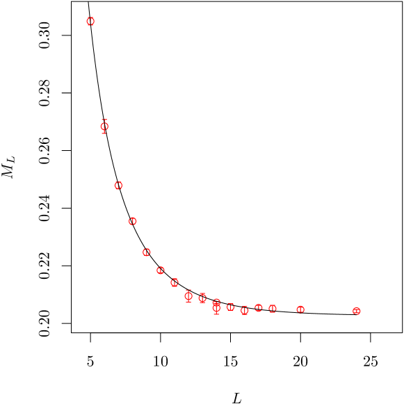
Figure 3: $M_{L}$ as a function of $L$. The solid line represents a fit of Eq. (18) to the data in the fit range $[4,24]$.

We now address the analysis of the lattice spectrum in our model, which is shown in Table 2 in Appendix A. Moreover, as an illustration we also show in Appendix B the plots for the effective mass and the correlation function for the case $L=18$.

First, we study the volume dependence of the single particle mass, which is given by Eq. (18). The results are range-independent and seem to describe the data very well. This is immediately seen in Fig. 3, which displays the fit of Eq. (18) to the data on $M_{L}$ in the whole range of volumes from $L_{\mathrm{min}}=4$ to $L_{\mathrm{max}}=24$. The fit yields

$$M_{\infty}=0.2027(2),\ \ \ \chi^{2}/\mathrm{d.o.f.}=15.17/16,\ \ \ p\,\text{-value}=0.44\,,$$ (38)

indicating a very good description of the data. The best fit parameters for the fits with other fit ranges are compiled in Appendix D.

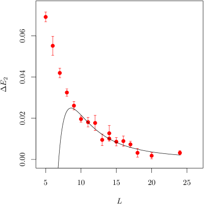
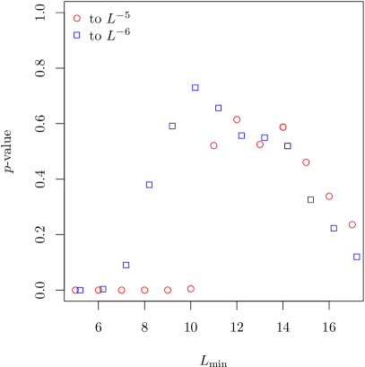
Figure 4: Left: fit of Eq. (20) to the data for $\Delta E_{2}$ in the $L$-range $[9,24]$ including $a$ and $r$ as fit parameters. Right: $p$-value of the fit of Eq. (20) to the data for $\Delta E_{2}$ as a function of $L_{\mathrm{min}}$ with a constant $L_{\mathrm{max}}=24$.

Next, we consider the two-particle energy shift $\Delta E_{2}(L)$, for which data from $L=4$ to $L=24$ are available. We fit Eq. (20) to the data, varying the lower end of the fit range in $L$ and the number of the fit parameters. The upper end in the fit range is kept fixed at $L_{\mathrm{max}}=24$. For large $L_{\mathrm{min}}$, one expects that only the scattering length is important and that in Eq. (20) one can neglect all terms of order $L^{-6}$ or smaller. Adding the effective range $r$ as a fit parameter, it should be possible to include smaller values of $L$ in the fit, while reproducing the results of the fit with only the scattering length as a free parameter.

In the left panel of Fig. 4, we show an example of a fit of Eq. (20) to the data including all terms up to order $L^{-6}$, i.e. with $a$ and $r$ as fit parameters. $L_{\mathrm{min}}=9$ was chosen for this particular fit. In the right panel of that figure, we show the $p$-value of the fit of Eq. (20) to the data as a function of $L_{\mathrm{min}}$. Red circles correspond to the one-parameter fit up to order $L^{-5}$, and blue squares to the two-parameter fit up to order $L^{-6}$. For the former, we observe the $p$-values around $0.5$ from $L_{\mathrm{min}}=11$ and larger, for the latter from around $L_{\mathrm{min}}=8$.

From these $L_{\mathrm{min}}$ values on, we also observe stable values for the fit parameters $a$ and $r$ within errors. This is shown in Fig. 5, where we plot $a$ in the left panel and $r$ in the right panel, both as functions of $L_{\mathrm{min}}$. In addition, as one infers from the left panel, the values for $a$ agree within errors between the single- and the two-parameter fits from the aforementioned $L_{\mathrm{min}}$-values onward. As a result, we quote here the best fit parameters from the two-parameter fit with $L_{\mathrm{min}}=9$, which can be found in Table 1.

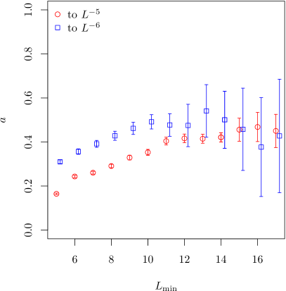
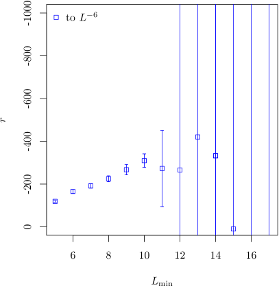
Figure 5: The scattering length $a$ (left) and the effective range $r$ (right) determined by a fit of Eq. (20) to the data for $\Delta E_{2}$ as functions of $L_{\mathrm{min}}$ with fixed $L_{\mathrm{max}}=24$.

Further, each data point for $\Delta E_{2}$ can be translated into one phase shift at a certain value of the scattering momentum. For that, we calculate the S-wave phase shift as Luescher-torus

$$\cot\delta=\frac{Z_{00}(1,q^{2})}{\pi^{3/2}q}\,,$$ (39)

where $Z_{00}(1,q^{2})$ is the generalized Lüscher zeta-function, $q=\frac{Lk}{2\pi}$ and $E_{2}=2\sqrt{k^{2}+M_{L}^{2}}$. Note that we used here the mass $M_{L}$, taking into account the discussion in Section III. The results can be seen from Table 3 in Appendix C. The phase shift obeys the inequality $|\delta|<2\,^{\circ}$, guaranteeing that with the current model parameters we are in the perturbative regime. The smallness of the phase shift also supports the validity of the arguments in Section III.

In Fig. 6, the phase shift is shown as a function of the scattering momentum $k$. We are now able to check, whether the parameters obtained from the fit to $\Delta E_{2}$ also describe the phase shift data properly. For this purpose, we use the effective range expansion:

$$k\cot\delta=-\frac{1}{a}+\frac{1}{2}rk^{2}+O(k^{4})$$ (40)

with the best fit parameters compiled in Table 1. In Figure 6, we show the phase shift (in degrees), determined by using Eq. (39), as a function of the scattering momentum $k$ (in lattice units). In addition, we show $\delta(k)$, determined from Eq. (40) by using the best fit parameters from the fit to $\Delta E_{2}$ (the solid line in this figure). It can be observed that both data analysis methods match nicely.

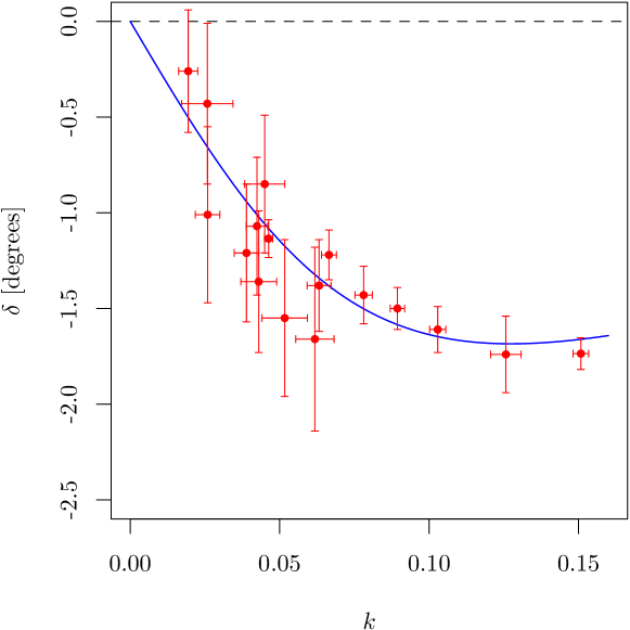
Figure 6: Phase shift as a function of the scattering momentum $k$ in lattice units. The expected curve, given by the parameters from the best fit to $\Delta E_{2}$, is shown as a solid line.

Turning to $\Delta E_{3}$ now, we have checked first that the data for the ratio

$$\frac{\Delta E_{3}}{\Delta E_{2}}=3+O(L^{-5}).$$ (41)

is close to $3$, as one expects. This is shown in the left panel of Fig. 7. Next we fit Eq. (21) to the data for $\Delta E_{3}$, including only the scattering length $a$ as a single fit parameter. Therefore, we include only the terms up to the order $L^{-5}$ in the fit. If everything is consistent, this should allow us to reproduce the value of the scattering length, determined by the fits to $\Delta E_{2}$ for sufficiently large values of $L_{\mathrm{min}}$.

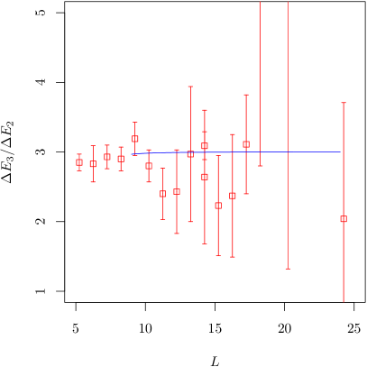
Figure 7: Left: Ratio $\Delta E_{3}/\Delta E_{2}$ as a function of $L$. The solid line represents the ratio computed from the best fit parameters from Table 1, using Eqs. (20) and (21). Right: Scattering length $a$ as a function of $L_{\mathrm{min}}$ determined fits of Eq. (21) up to order $L^{-5}$ to our data for $\Delta E_{3}$, i.e. with $a$ the only fit parameter.

The result of this exercise is shown in the left panel of Fig. 7 and the right panel of Fig. 8. We plot $a$ and the $p$-value of the fit, both as functions of $L_{\mathrm{min}}$. We observe reasonable $p$-values from $L_{\mathrm{min}}=11$ onward and the best fit values for $a$ lie between $0.4$ and $0.5$. Within errors, this is in agreement with the value quoted in Table 1, which was obtained from the fit to $\Delta E_{2}$. We hence conclude that, for sufficiently large values of $L$, the data for $\Delta E_{3}$ and $\Delta E_{2}$ are reasonably well described by the same value of the scattering length $a$. We cannot perform the same test, including also $r$, because at that order also the three-body term contributes.

As a next step, we will use the results for $a$ and $r$ from the fit of Eq. (20) to the data for $\Delta E_{2}$ as priors for the fit of Eq. (21) to the data for $\Delta E_{3}$, including terms up to the order $L^{-6}$. To this end, we introduce an augmented $\chi^{2}$ function

$$\chi^{2}_{\mathrm{aug}}\ =\ \chi^{2}+\left(\frac{P_{r}-r}{\Delta r}\right)^{2}+\left(\frac{P_{a}-a}{\Delta a}\right)^{2}$$

with $\chi^{2}$ defined as usual, $P_{r}$ and $P_{a}$ being the priors for $a$ and $r$, respectively, and $\Delta a$ and $\Delta r$ denoting the corresponding standard errors. In the fit, we minimize the augmented $\chi^{2}_{\mathrm{aug}}$. The actual values for $P_{a},P_{r},\Delta a$ and $\Delta r$ are the best fit parameters with errors, which can be found in Table 1. The goal here is to see whether we get a significant contribution from the three-body term in Eq. (21) or not. An example of a fit with $L_{\mathrm{min}}=9$ and $L_{\mathrm{max}}=24$ is shown in the right panel of Fig. 8.

Figure 8: Left: $p$-value as a function of $L_{\mathrm{min}}$ for the fits of Eq. (21) up to order $L^{-5}$ to our data for $\Delta E_{3}$, i.e. with $a$ the only fit parameter. Right: Exemplary plot of a fit (solid line) of Eq. (21) to the data for $\Delta E_{3}$ with $L_{\mathrm{min}}=9$ and $L_{\mathrm{max}}=24$.

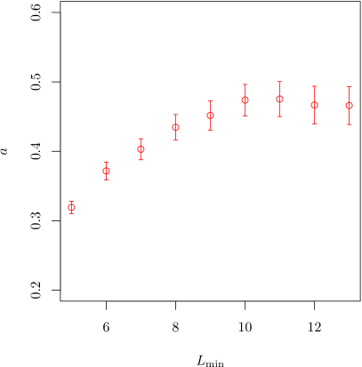
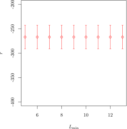
Figure 9: $a$ and $r$ as functions of $L_{\mathrm{min}}$ from the fits of Eq. (21) to the data for $\Delta E_{3}$. Both $a$ and $r$ were included in the fit with priors from the fit to $\Delta E_{2}$ (the values can be found in Table 1).

The scattering length $a$ and the effective range $r$ are highly constrained by the prior included in the fit. This can be observed from Fig. 9, where $a$ (left panel) and $r$ (right panel) are plotted as functions of $L_{\mathrm{min}}$. The fit to $\Delta E_{3}$ appears not to be sensitive to the effective range $r$, with the prior value always reproduced. This is expected, because the term proportional to $r$ interferes with the term proportional to $D$. Thus, the fit will always choose the prior value for $r$ to minimize the augmented $\chi^{2}$. For $a$, we again observe that, for sufficiently large $L_{\mathrm{min}}$, the value from the fit to $\Delta E_{2}$ is reproduced within errors. From this, one may infer that $L_{\mathrm{min}}\geq 9$ should be chosen.

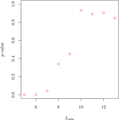
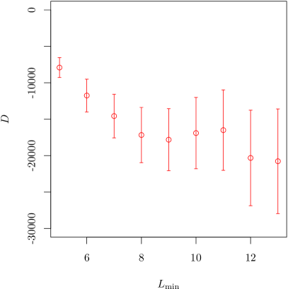
Figure 10: $p$-value and $D$ as functions of $L_{\mathrm{min}}$ from fits of Eq. (21) to the data of $\Delta E_{3}$.

This conclusion is also supported by the $p$-value, shown in the left panel of Fig. 10 as a function of $L_{\mathrm{min}}$. For $L_{\mathrm{min}}=8$ and $9$ we observe reasonable $p$-values. For $L_{\mathrm{min}}=10$ or larger the $p$-values become close to $1$, indicating at too many fit parameters for too few data points. Finally, in the right panel of Fig. 10, we show the three-body parameter $D$ as a function of $L_{\mathrm{min}}$. In the relevant region of $L_{\mathrm{min}}$ we observe a plateau within errors at a value significantly different from zero. Actually, $D$ is different from zero to many $\sigma$ for all considered values of $L_{\mathrm{min}}$, in particular $4\sigma$ for $L_{\mathrm{min}}=9$. Final results of the fit to $\Delta E_{3}$ are shown in Table 1.

	$[L_{\mathrm{min}},L_{\mathrm{max}}]$	$a$	$r$	$D$	$\chi^{2}/\mathrm{d.o.f.}$	$p$-value
$\Delta E_{2}$	[9,24]	0.46(3)	-267(24)	—	9.33/10	0.59
$\Delta E_{3}$	[9,24]	0.45(2)	-267(24)	-17814(4378)	10.90/11	0.45

Table 1: Selected fit results to $\Delta E_{2,3}$

Eventually, we can use the parameters from Table 1 to compute the ratio $\Delta E_{3}/\Delta E_{2}$, using Eqs. (20) and (21), both to the order $L^{-6}$. The result is shown as a solid line in the left panel of Fig. 7. The agreement is satisfactory within error bars.

We close this section with two remarks: First, we have also included an effective term of order $L^{-7}$ in the fits and observed that our results are stable under such a change. Second, a direct fit to the data for $\Delta E_{3}/\Delta E_{2}$ appears not to be sensitive to the fit parameters we are interested in.

V Summary and Outlook

In this paper, we have investigated the two- and three-particle interactions in complex $\varphi^{4}$ theory on the lattice. In particular, we have carried out a theoretical study of the exponential finite-volume corrections to the one-, two- and three-particle energy levels. To next-to-leading order in perturbation theory it was shown that, using the finite-volume particle mass $M_{L}$ instead of the infinite-volume one $M$ in the definition of the two- and three-particle threshold energies allows one to significantly reduce the exponential corrections to the Lüscher-type formulae for the two- and three-particle ground-state energy shifts. For example, in case of the model considered, these corrections get a suppression factor $\lambda_{c}/L^{2}$, when $M_{L}$ is used. A proof of this statement to all orders in perturbation theory seems challenging but worth trying, since it could be interesting for many lattice QCD applications. We plan to take up this challenge in our future publications.

The big advantage of $\varphi^{4}$ theory as compared to QCD lies in a much reduced computational complexity. This fact allowed us to study a large set of ensembles with different finite volumes at fixed values of bare parameters. At the first stage, we study the finite-volume corrections to the single-particle mass on these ensembles. We show that these corrections are well described by the corresponding expression known from the effective field theory. Next, for each of the aforementioned ensembles, we determine the two-particle and three-particle energy shifts in a finite volume, $\Delta E_{2}$ and $\Delta E_{3}$. Then, we extract the scattering length $a$ and the effective range $r$ from the $L$-dependence of $\Delta E_{2}$ by applying the Lüscher formalism. We also show that, depending on the range of values of $L$, used in the fit, either only $a$ or $a$ and $r$ together can be determined, with consistent results for $a$ in both cases.

As a next step, we show that we can extract the scattering length for sufficiently large values of $L$ from $\Delta E_{3}$ as well, and its value turns out to be consistent with the value extracted from the fit to $\Delta E_{2}$. Hence, we conclude that our data for $\Delta E_{2}$ and $\Delta E_{3}$ are consistent. Now, we follow the idea of Refs. pang1 ; pang2 and use $a$ (and $r$), determined from $\Delta E_{2}$, as an input for the analysis of $\Delta E_{3}$. In this case, the (higher order) formula for $\Delta E_{3}$ includes the three-body effective coupling as well. On the basis of the analysis of data, taken at many different volumes, we find a statistically significant three-body contribution $D$, which is definitely away from zero. This is a central result of our work.

In this simple theory, there are still many issues to be explored. For example, one could study the multiparticle states with more than three particles and try to figure out, how their energy depends on the volume. Moreover, one may include excited three-particle states in the rest frame or moving frames for a more sophisticated study of the three-body coupling. In addition, it would be interesting to investigate $\varphi^{4}$ theory at parameter values where a the three-body bound state is present, since the volume-dependence of such an energy level is qualitatively different from the one seen it this work. For this, one would have to further explore the parameter space of the theory.

Appendix A Spectrum

$L$	$T$	$n_{conf}$	$M_{L}$	$E_{2}(L)$	$E_{3}(L)$	$\Delta E_{2}$	$\Delta E_{3}$	$\Delta E_{3}/\Delta E_{2}$
4	24	18000	0.3634(16)	–	–	–	–	–
5	24	28000	0.3049(13)	0.6790(20)	1.1121(93)	0.0692(24)	0.1973(97)	2.85(12)
6	24	7500	0.2684(24)	0.5920(36)	0.962(16)	0.0552(46)	0.156(17)	2.83(26)
7	24	30000	0.2479(12)	0.5378(17)	0.8669(74)	0.0420(23)	0.1233(79)	2.93(17)
8	24	47000	0.2355(10)	0.5035(13)	0.8006(57)	0.0325(18)	0.0941(62)	2.90(17)
9	24	40000	0.2247(11)	0.4756(14)	0.7574(62)	0.0261(20)	0.0832(67)	3.19(24)
10	24	70000	0.21843(85)	0.4565(11)	0.7103(46)	0.0196(15)	0.0550(50)	2.80(23)
11	24	30000	0.2142(13)	0.4464(17)	0.6859(71)	0.0181(23)	0.0434(77)	2.40(37)
12	24	12000	0.2095(21)	0.4367(26)	0.672(11)	0.0177(37)	0.043(12)	2.43(60)
13	24	20000	0.2088(16)	0.4271(21)	0.6546(91)	0.0095(28)	0.0282(98)	2.97(97)
14	24	28000	0.2054(22)	0.4236(28)	0.650(13)	0.0127(38)	0.034(14)	2.64(96)
15	24	40000	0.2057(12)	0.4199(15)	0.6362(66)	0.0086(20)	0.0192(70)	2.23(72)
16	24	52000	0.2045(14)	0.4179(18)	0.6347(83)	0.0089(25)	0.0211(88)	2.37(88)
17	24	70000	0.20540(87)	0.4181(11)	0.6388(50)	0.0073(15)	0.0226(54)	3.11(71)
18	24	36000	0.2051(12)	0.4134(16)	0.6371(71)	0.0032(21)	0.0218(76)	6.8(4.0)
20	24	70000	0.20477(87)	0.4114(11)	0.6241(52)	0.0018(15)	0.0098(55)	5.4(4.1)
14	48	36000	0.20724(33)	0.42461(63)	0.6530(23)	0.01014(62)	0.0313(24)	3.09(20)
24	48	100000	0.20426(55)	0.4118(11)	0.6194(58)	0.0032(10)	0.0066(59)	2.0(1.7)

Table 2: Energies, obtained from the lattice for one, two and three particles. Moreover, we include the energy difference and the ratio treating the correlations in a proper way.

Appendix B Effective mass and Correlation functions for $L=18$

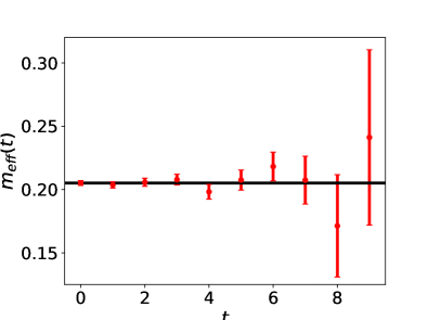
(a)  Effective mass for one particle at $L=18$.

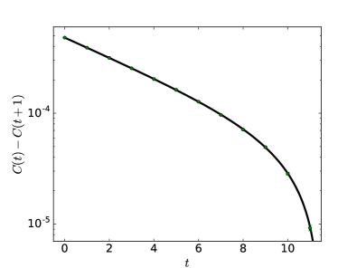
(b)  Correlation function of one particle for $L=18$

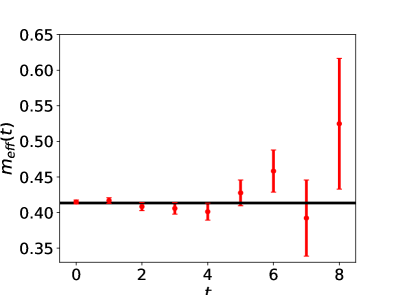
(c)  Effective mass for two particles in $L=18$.

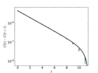
(d)  Correlation function of two particles for $L=18$

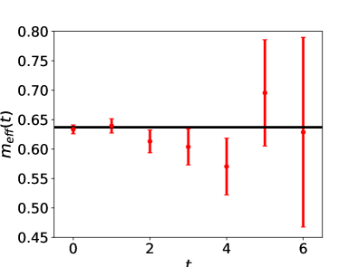
(e)  Effective mass for three particle in $L=18$.

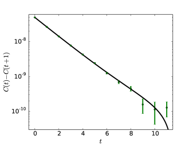
(f)  Correlation function of three particles for $L=18$

Figure 11: Relevant plots for our analysis at $L=18$

Appendix C Phase Shifts

$L$	$T$	$k$	${\delta}$
5	24	0.1508(26)	-1.736(83)
6	24	0.1257(51)	-1.74(20)
7	24	0.1029(27)	-1.61(12)
8	24	0.0894(24)	-1.50(11)
9	24	0.0781(29)	-1.43(15)
10	24	0.0665(25)	-1.22(13)
11	24	0.0632(40)	-1.38(24)
12	24	0.0618(64)	-1.66(48)
13	24	0.0450(67)	-0.85(36)
14	24	0.0517(76)	-1.55(41)
15	24	0.0424(36)	-1.07(36)
16	24	0.0430(60)	-1.36(37)
17	24	0.0389(41)	-1.21(36)
18	24	0.0258(86)	-0.43(42)
20	24	0.0194(32)	-0.26(32)
24	48	0.0259(41)	-1.01(46)
14	48	0.0463(14)	-1.135(99)

Table 3: Phase shift in degrees, obtained from Eq. (39). The small value ensures perturbability.

Appendix D Fits $\Delta E_{2,3}$

$[L_{i},L_{f}]$	$a$	$r$	$\chi^{2}/\mathrm{d.o.f.}$	$p$-value
$[7,24]$	0.391(16)	-191(10)	1.55	0.09
$[8,24]$	0.428(20)	-225(14)	1.07	0.38
$[9,24]$	0.462(28)	-267(24)	0.84	0.59
$[10,24]$	0.491(32)	-309(32)	0.70	0.73
$[11,24]$	0.477(51)	-270(180)	0.76	0.66

Table 4: Exemplary fit results for $\Delta E_{2}$.

$[L_{i},L_{f}]$	$a$	$D$	$\chi^{2}/\mathrm{d.o.f.}$	$p$-value
$[7,24]$	0.403(15)	-14569(3022)	1.75	0.04
$[8,24]$	0.435(18)	-17169(3915)	1.12	0.34
$[9,24]$	0.452(21)	-17814(4378)	0.99	0.45
$[10,24]$	0.474(23)	-16903(5030)	0.43	0.93
$[11,24]$	0.475(25)	-16502(5592)	0.48	0.89

Table 5: Exemplary fit results for $\Delta E_{3}$.

References

- (1) M. Lüscher, Nucl. Phys. B 354 (1991) 531.
- (2) K. Rummukainen and S. A. Gottlieb, Nucl. Phys. B 450 (1995) 397 [hep-lat/9503028].
- (3) M. Lage, U.-G. Meißner and A. Rusetsky, Phys. Lett. B 681 (2009) 439 [arXiv:0905.0069 [hep-lat]].
- (4) V. Bernard, M. Lage, U.-G. Meißner and A. Rusetsky, JHEP 1101 (2011) 019 [arXiv:1010.6018 [hep-lat]].
- (5) C. Liu, X. Feng and S. He, JHEP 0507 (2005) 011 [arXiv:hep-lat/0504019]; Int. J. Mod. Phys. A 21 (2006) 847, [arXiv:hep-lat/0508022].
- (6) M. T. Hansen and S. R. Sharpe, Phys. Rev. D 86 (2012) 016007 [arXiv:1204.0826 [hep-lat]].
- (7) R. A. Briceño and Z. Davoudi, Phys. Rev. D 88 (2013) 094507 [arXiv:1204.1110 [hep-lat]].
- (8) N. Li and C. Liu, Phys. Rev. D 87 (2013) 014502 [arXiv:1209.2201 [hep-lat]].
- (9) P. Guo, J. Dudek, R. Edwards and A. P. Szczepaniak, Phys. Rev. D 88 (2013) 014501 [arXiv:1211.0929 [hep-lat]].
- (10) C. Morningstar, J. Bulava, B. Singha, R. Brett, J. Fallica, A. Hanlon and B. Hörz, Nucl. Phys. B 924 (2017) 477 [arXiv:1707.05817 [hep-lat]].
- (11) C. Helmes, C. Jost, B. Knippschild, B. Kostrzewa, L. Liu, C. Urbach and M. Werner, Phys. Rev. D 96 (2017) no.3, 034510 [arXiv:1703.04737 [hep-lat]].
- (12) L. Liu et al., Phys. Rev. D 96 (2017) no.5, 054516 [arXiv:1612.02061 [hep-lat]].
- (13) C. Helmes et al. [ETM Collaboration], JHEP 1509 (2015) 109 [arXiv:1506.00408 [hep-lat]].
- (14) F. Romero-López, A. Rusetsky and C. Urbach, arXiv:1802.03458 [hep-lat].
- (15) J. J. Dudek et al. [Hadron Spectrum Collaboration], Phys. Rev. Lett. 113 (2014) 182001 [arXiv:1406.4158 [hep-ph]]; D. J. Wilson, J. J. Dudek, R. G. Edwards and C. E. Thomas, Phys. Rev. D 91 (2015) 054008 [arXiv:1411.2004 [hep-ph]]; J. J. Dudek et al. [Hadron Spectrum Collaboration], Phys. Rev. D 93 (2016) 094506 [arXiv:1602.05122 [hep-ph]].
- (16) D. R. Bolton, R. A. Briceño and D. J. Wilson, Phys. Lett. B 757 (2016) 50 [arXiv:1507.07928 [hep-ph]].
- (17) R. A. Briceño, J. J. Dudek, R. G. Edwards and D. J. Wilson, Phys. Rev. Lett. 118, 022002 (2017) [arXiv:1607.05900 [hep-ph]].
- (18) R. A. Briceno, J. J. Dudek, R. G. Edwards and D. J. Wilson, Phys. Rev. D 97 (2018) 054513 [arXiv:1708.06667 [hep-lat]].
- (19) D. Guo, A. Alexandru, R. Molina, M. Mai and M. Döring, arXiv:1803.02897 [hep-lat].
- (20) L. Lellouch and M. Lüscher, Commun. Math. Phys. 219 (2001) 31 [hep-lat/0003023].
- (21) M. T. Hansen and S. R. Sharpe, Phys. Rev. D 86 (2012) 016007 [arXiv:1204.0826 [hep-lat]].
- (22) R. A. Briceño, M. T. Hansen and A. Walker-Loud, Phys. Rev. D 91 (2015) 3, 034501 [arXiv:1406.5965 [hep-lat]].
- (23) R. A. Briceño and M. T. Hansen, Phys. Rev. D 92 (2015) 7, 074509, [arXiv:1502.04314 [hep-lat]].
- (24) V. Bernard, D. Hoja, U.-G. Meißner and A. Rusetsky, JHEP 1209 (2012) 023 [arXiv:1205.4642 [hep-lat]].
- (25) A. Agadjanov, V. Bernard, U.-G. Meißner and A. Rusetsky, Nucl. Phys. B 886 (2014) 1199 [arXiv:1405.3476 [hep-lat]].
- (26) A. Agadjanov, V. Bernard, U.-G. Meißner and A. Rusetsky, Nucl. Phys. B 910 (2016) 387 [arXiv:1605.03386 [hep-lat]].
- (27) R. A. Briceño, J. J. Dudek, R. G. Edwards, C. J. Shultz, C. E. Thomas and D. J. Wilson, Phys. Rev. D 93 (2016) 114508 [arXiv:1604.03530 [hep-ph]].
- (28) K. Polejaeva and A. Rusetsky, Eur. Phys. J. A 48 (2012) 67, [arXiv:1203.1241 [hep-lat]].
- (29) U.-G. Meißner, G.-Rios and A. Rusetsky, Phys. Rev. Lett. 114 (2015) 091602 Erratum: [Phys. Rev. Lett. 117 (2016) 069902], [arXiv:1412.4969 [hep-lat]].
- (30) P. Guo, Phys. Rev. D 95 (2017) 054508, [arXiv:1607.03184 [hep-lat]].
- (31) P. Guo and V. Gasparian, Phys. Lett. B 774 (2017) 441 [arXiv:1701.00438 [hep-lat]].
- (32) R. A. Briceño and Z. Davoudi, Phys. Rev. D 87 (2013) 094507, [arXiv:1212.3398 [hep-lat]].
- (33) M. T. Hansen and S. R. Sharpe, Phys. Rev. D 90 (2014) 116003, [arXiv:1408.5933 [hep-lat]].
- (34) M. T. Hansen and S. R. Sharpe, Phys. Rev. D 92 (2015) 114509, [arXiv:1504.04248 [hep-lat]].
- (35) M. T. Hansen and S. R. Sharpe, Phys. Rev. D 93 (2016) 014506, [arXiv:1509.07929 [hep-lat]].
- (36) M. T. Hansen and S. R. Sharpe, Phys. Rev. D 93 (2016) 096006, [arXiv:1602.00324 [hep-lat]].
- (37) M. T. Hansen and S. R. Sharpe, Phys. Rev. D 95 (2017) 034501, [arXiv:1609.04317 [hep-lat]].
- (38) R. A. Briceño, M. T. Hansen and S. R. Sharpe, Phys. Rev. D 95 (2017) 074510 [arXiv:1701.07465 [hep-lat]].
- (39) S. Kreuzer and H.-W. Hammer, Phys. Lett. B 694 (2011) 424, [arXiv:1008.4499 [hep-lat]].
- (40) S. Kreuzer and H.-W. Hammer, Eur. Phys. J. A 43 (2010) 229, [arXiv:0910.2191 [nucl-th]].
- (41) S. Kreuzer and H.-W. Hammer, Phys. Lett. B 673 (2009) 260, [arXiv:0811.0159 [nucl-th]].
- (42) S. Kreuzer and H.-W. Grießhammer, Eur. Phys. J. A 48 (2012) 93, [arXiv:1205.0277 [nucl-th]].
- (43) S. R. Sharpe, Phys. Rev. D 96 (2017) 054515 [arXiv:1707.04279 [hep-lat]].
- (44) H.-W. Hammer, J. Y. Pang and A. Rusetsky, JHEP 1709 (2017) 109 [arXiv:1706.07700 [hep-lat]].
- (45) H.-W. Hammer, J.-Y. Pang and A. Rusetsky, JHEP 1710 (2017) 115 [arXiv:1707.02176 [hep-lat]].
- (46) Y. Meng, C. Liu, U.-G. Meißner and A. Rusetsky, arXiv:1712.08464 [hep-lat].
- (47) M. Döring, H.-W. Hammer, M. Mai, J.-Y. Pang, A. Rusetsky and J. Wu, arXiv:1802.03362 [hep-lat].
- (48) M. Mai and M. Döring, Eur. Phys. J. A 53 (2017) 240 [arXiv:1709.08222 [hep-lat]].
- (49) R. A. Briceño, M. T. Hansen and S. R. Sharpe, arXiv:1803.04169 [hep-lat].
- (50) P. F. Bedaque, H.-W. Hammer and U. van Kolck, Phys. Rev. Lett. 82 (1999) 463 [nucl-th/9809025].
- (51) P. F. Bedaque, H.-W. Hammer and U. van Kolck, Nucl. Phys. A 646 (1999) 444 [nucl-th/9811046].
- (52) E. Epelbaum, J. Gegelia, U.-G. Meißner and D. L. Yao, Eur. Phys. J. A 53 (2017) 98 [arXiv:1611.06040 [nucl-th]].
- (53) S. R. Beane, W. Detmold, T. C. Luu, K. Orginos, M. J. Savage and A. Torok, Phys. Rev. Lett. 100 (2008) 082004 [arXiv:0710.1827 [hep-lat]].
- (54) W. Detmold, M. J. Savage, A. Torok, S. R. Beane, T. C. Luu, K. Orginos and A. Parreno, Phys. Rev. D 78 (2008) 014507 [arXiv:0803.2728 [hep-lat]].
- (55) C. Gattringer, M. Giuliani and O. Orasch, arXiv:1804.01580 [hep-lat].
- (56) K. Huang and C. N. Yang, Phys. Rev. 105 (1957) 767.
- (57) T. T. Wu, Phys. Rev. 115 (1959) 1390.
- (58) S. Tan, Phys. Rev. A 78 (2008) 013636 [arXiv:0709.2530 [cond-mat.stat-mech]].
- (59) S. R. Beane, W. Detmold and M. J. Savage, Phys. Rev. D 76 (2007) 074507 [arXiv:0707.1670 [hep-lat]].
- (60) J.-Y. Pang, J. Wu, H.-W. Hammer, U.-G. Meißner and A. Rusetsky, in preparation.
- (61) K. Ottnad et al. [ETM Collaboration], Phys. Rev. D 97 (2018) 054508 [arXiv:1710.07986 [hep-lat]].
- (62) J. Gasser and H. Leutwyler, Phys. Lett. B 184 (1987) 83.
- (63) G. Colangelo and S. Durr, Eur. Phys. J. C 33 (2004) 543 [hep-lat/0311023]; G. Colangelo, S. Durr and C. Haefeli, Nucl. Phys. B 721 (2005) 136 [hep-lat/0503014].
- (64) M. Lüscher, Commun. Math. Phys. 104 (1986) 177.