Spin liquid fingerprints in the thermal transport of a Kitaev-Heisenberg ladder

Abstract

We identify fingerprints of a proximate quantum spin-liquid (QSL), observable by finite-temperature dynamical thermal transport within a minimal version of the idealized Kitaev model on a two-leg ladder, if subjected to inevitably present Heisenberg couplings. Using exact diagonalization and quantum typicality, we uncover (i) an insulator-conductor crossover induced by fracton recombination at infinitesimal Heisenberg coupling, (ii) low- and high-energy signatures of fractons, which survive far off the pure QSL point, and (iii) a non-monotonous current life-time versus Heisenberg couplings. Guided by perturbation theory, we find (iv) a Kitaev-exchange induced “one-magnon” contribution to the dynamical heat transport in the strong Heisenberg rung limit.

A quantum spin liquid (QSL) is an elusive state of magnetic matter with the intriguing property of lacking a local magnetic order parameter in the absence of external fields at any temperature $T$ Savary and Balents (2017); Zhou et al. (2017). Instead, QSLs may show quantum orders, massive entanglement and exotic fractional elementary excitations, e.g. spinons Coldea et al. (2001); Helton et al. (2007); Gomilšek et al. (2017), Majorana fermions, gauge vortices Hermanns et al. (2015); Le Hur et al. (2017) and alike. QSLs are a consequence of frustrating exchange couplings, such that the local magnetic moments cannot simultaneously satisfy their mutual interactions Lee (2014). In a seminal paper Kitaev (2006), Kitaev introduced an exactly solvable $\mathbb{Z}_{2}$ QSL-model, where spin-$1/2$ operators reside on the vertices of a honeycomb lattice and are subject to exchange frustration from Ising interactions of the type $XX$, $YY$, or $ZZ$ depending on the direction of the bond Hermanns et al. (2018). Early on, it was proposed that such patterns can be realized in optical lattices Duan et al. (2003), and shortly after also in Mott-Hubbard insulators with strong spin orbit coupling (SOC) Jackeli and Khaliullin (2009); Chaloupka et al. (2010). In the quest for materials which host Kitaev physics, several compounds have surfaced, e.g. the iridates $\alpha$-$\mathrm{Na_{2}IrO_{3}}$ or $\alpha$-$\mathrm{Li_{2}IrO_{3}}$, as well as $\alpha$-$\mathrm{RuCl_{3}}$. The latter systems, however, all order magnetically at low temperatures due to additional interactions Yadav et al. (2016); Choi et al. (2012); Nishimoto et al. (2016); Ye et al. (2012). Recently, $\mathrm{H_{3}LiIr_{2}O_{6}}$ has been synthesized, which reportedly shows no magnetic order at temperatures $\gtrsim 10^{-4}J$, with $J$ the exchange interaction Kitagawa et al. (2018).

With low-$T$ magnetic ordering being the common obstacle in real materials, preempting the putative formation of a QSL, it is of tantamount importance to identify and interpret fingerprints, genuine to a QSL in systems which are subject to residual interactions, which obscure QSL behavior. For Kitaev magnets, this is not trivial and largely under debate Banerjee et al. (2016); Sandilands et al. (2015); Glamazda et al. (2017); Winter et al. (2018); Nasu et al. (2016); Winter et al. (2017). In this endeavor, thermal transport has also been employed. Unlike to other magnetic systems Hess et al. (2003); Hlubek et al. (2010), the longitudinal thermal conductivity $\kappa_{xx}$ in $\alpha$-$\mathrm{RuCl_{3}}$ is predominantly phononic with, however, a very unusual behavior Hirobe et al. (2017); Yu et al. (2018); Hentrich et al. (2018); Leahy et al. (2017); Hentrich et al. (2018). Whether this is due to remnants of Majorana fermions is not clear. Stronger evidence of Kitaev physics might show up in finite external magnetic fields (not considered here), because the low temperature magnetic order is suppressed Baek et al. (2017) and it could give rise to a quantized thermal Hall conductance Kasahara et al. (2018).

Theoretically, thermal transport studies in pure Kitaev QSLs have been performed via quantum Monte Carlo simulations in 2D Nasu et al. (2017) or via ED in 1D and 2D Metavitsiadis and Brenig (2017); Metavitsiadis et al. (2017). Moment expansions might also provide high-temperature analytic results for thermal transport of pure Kitaev QSLs in the future Briffa and Zotos (2018). Thermal transport was also studied in magnetically ordered phases of a Kitaev-Heisenberg model using spin wave calculations Stamokostas et al. (2017). However, the impact of isotropic Heisenberg exchange on thermal transport, perturbing a pure Kitaev QSL, is a completely open issue. Here our work makes a step forward. We study the thermal transport properties of a Kitaev-Heisenberg ladder (KHL), using exact diagonalization (ED), dynamical quantum typicality (DQT), and perturbation theory. By tuning the exchange between the limits of a pure Kitaev ladder (KL) and a Heisenberg ladder (HL), we provide a comprehensive view on the transport properties, while crossing over from a $\mathbb{Z}_{2}$ QSL into a conventional dimer magnet with gapped triplon excitations. En route, we emphasize characteristics which serve to identify Kitaev physics even at moderate Heisenberg couplings.

The Hamiltonian for the Kitaev-Heisenberg model on a ladder of $L$ rungs with boundary conditions is given by

$$H=\sum_{a=x,y,z}\sum_{\langle i,j\rangle}J_{ij}^{a}S_{i}^{a}S_{j}^{a}+J_{ij}S_{i}^{a}S_{j}^{a}~{}.$$ (1)

Here $S$ are spin-$1{/}2$ operators, and the restricted sum over $i,j$ reproduces the geometry depicted in Fig. 1. $J_{ij}^{a}=J_{x},J_{y},J_{z}$ denote the anisotropic Kitaev interactions–only one of them is non-zero per bond–which we parametrize in terms of the coupling strength $J_{K}$. On the other hand, $J_{ij}=J_{H},J_{H}^{\prime}$ are $\mathrm{SU(2)}$ invariant Heisenberg interactions. If $J_{H}\neq J_{H}^{\prime}$ is considered we will note this explicitly. Lastly, we set the lattice constant equal to unity, as well as the Planck and Boltzmann constants.

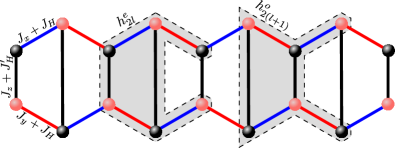
Figure 1: The Kitaev-Heisenberg ladder. $J_{x}$, $J_{y}$, and $J_{z}$ denote Ising interactions, while $J_{H}$ and $J_{H}^{\prime}$ $\mathrm{SU(2)}$ invariant Heisenberg interactions. The local energy densities $h_{l}^{e}$ and $h_{l}^{o}$ used to define the energy current are highlighted.

In the absence of Heisenberg interactions ($J_{ij}=0$) the system is a $\mathbb{Z}_{2}$ spin liquid Feng et al. (2007); Wu (2012); Le Hur et al. (2017). The spin degrees of freedom fractionalize into two species of Majorana fermions and the Hamiltonian acquires the form Le Hur et al. (2017)

$$H=-\frac{i}{4}\sum_{b}J_{x}c_{b}c_{r}+J_{y}c_{b}c_{r}-J_{z}(i\bar{c}_{b}\bar{c}_{r})c_{b}c_{r}\,,$$ (2)

where $c,\bar{c}$ represent Majorana fermions, $\{c_{i},c_{j}\}=2\delta_{ij}=\{\bar{c}_{i},\bar{c}_{j}\}$, while the indices $b$ and $r$ correspond to the “black” and “red” sites of the lattice respectively. The quantity in the parenthesis is a good quantum number of the model, $\eta=i\bar{c}_{b}\bar{c}_{r}=\pm 1$, and therefore the $\bar{c}$ species becomes static. By defining Dirac fermions from pairs of Majorana fermions residing on the two sites of the same rung, Hamiltonian (2) transforms to a tight-binding chain with pairing terms in the presence of a $\mathbb{Z}_{2}$ gauge field, with the latter acting as a disorder potential. The ground state of the system lies in the uniform $\eta$-sectors, and it can either be gapless for $|J_{x}-J_{y}|=J_{z}$, or gapped otherwise. Further we emphasize that for $|J_{x}-J_{y}|>J_{z}$ the system acquires a finite topological (string-)order parameter Feng et al. (2007); Wu (2012).

Transport properties of the KL were analyzed in Ref. [35], showing that in this quasi-1D case, the sole carriers of heat, the Majorana fermions, scatter from the thermally activated static gauge disorder such, that localization occurs. I.e. the KL turns into an ideal heat insulator at all temperatures. In the pure 2D Kitaev model similar scattering occurs, but too weak to force localization, leading to normal heat conduction Nasu et al. (2017); Metavitsiadis et al. (2017). In contrast, the HL exhibits a ground state adiabatically connected to a rung-singlet product (RSP) state, and triplon excitations Dagotto and Rice (1996). The energy transport of the HL has been analyzed exhaustively over wide ranges of coupling strengths and temperatures and is well understood to be diffusive Zotos (2004); Steinigeweg et al. (2016).

To analyze the thermal transport properties of the KHL, we obtain the energy current operator $j^{\epsilon}$ from the time derivative of the polarization operator, $P^{\epsilon}=\sum_{l}2lh_{2l}$ Mahan (1981), which yields $j^{\epsilon}=-2i\sum_{l}[h_{2l},h_{2(l-1)}]$. The local energy density $h_{2l}$ satisfies the constraint $\sum_{l}h_{2l}=H$, rendering the choice of $h_{2l}$ not unique. In this work, we choose $h_{2l}=(h_{2l}^{e}+h_{2l}^{o})/2$, see Fig. 1. We emphasize, that such freedom of choice does not affect our main findings.

The real part of the energy current correlation function is given by $C(t)=\mathrm{Re}[\langle j^{\epsilon}(t)j^{\epsilon}\rangle/L]$, where the brackets $\langle\cdots\rangle$ denote the thermal expectation value at temperature $T$. The thermal Drude weight (DW) $D$ as well as the regular part $\kappa^{\prime}$ of the thermal conductivity, $\kappa(\omega)=2\pi D\delta(\omega)+\kappa^{\prime}(\omega)$, are obtained via

$$D=\frac{C_{0}}{2T^{2}},~{}\kappa^{\prime}(\omega)=\mathcal{P}\frac{2\beta}{\omega}\tanh\frac{\beta\omega}{2}\int_{0}^{\infty}dt\cos\omega t~{}C(t),$$ (3)

with $\beta=1/T$, $\mathcal{P}$ the principal value, and $C_{0}$ the time independent contribution of degenerate states to $C(t)$. The static value of the regular part is determined by the limiting procedure $\kappa_{dc}=\kappa^{\prime}(\omega\rightarrow 0)$. A finite value of $D$ signifies dissipationless energy transport, whereas the contribution of dissipative modes to the normal dc conductivity is obtained by $\kappa_{dc}$. In the case where $D$ and $\kappa_{dc}$ vanish simultaneously the system is an ideal heat insulator Zotos and Prelovšek (1996).

The thermal expectation value is evaluated numerically either using exact diagonalization (ED) by tracing over the full Hilbert space, or by using the dynamical quantum typicality (DQT), where the full trace is replaced by a scalar product of a pure random state $|\psi\rangle$, evolved to $|\psi_{\beta}\rangle=e^{-\beta H/2}|\psi\rangle$ to account for finite temperatures Steinigeweg et al. (2014). The limiting temperature for the DQT is approximately the energy scale of the system $J$, which is formally defined below Steinigeweg et al. (2016). The correlation function is then evaluated via $C(t)\approx\mathrm{Re}\frac{\langle\psi_{\beta}|j^{\epsilon}(t)j^{\epsilon}|\psi_{\beta}\rangle}{L\langle\psi_{\beta}|\psi_{\beta}\rangle}$ by solving a standard differential equation problem for the temperature and the time evolution. The error in DQT scales with the inverse square root of the Hilbert space dimension, namely exponentially with $L$. The time (temperature) evolution is performed with a $J\delta t=0.01$ ($J\delta\beta=0.01$) step [corresponding to an accuracy of the order of $O(10^{-8})$ in the fourth order Runge-Kutta algorithm], and up to a maximum time $t_{m}J=100\pi$, giving a $\pi/t_{m}=0.01J$ frequency resolution. We keep the same frequency resolution also for the ED results in the binning of the $\delta$ functions.

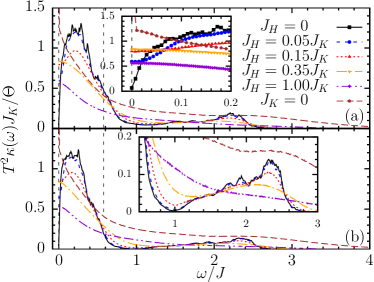
Figure 2: High temperature thermal conductivity versus frequency on a ladder of $L=12$ rungs via DQT for: (a) $J_{x,y,z}=(2,1,1)J_{K}$ and (b) $J_{x,y,z}=(3,1,1)J_{K}$. For each case the Heisenberg couplings $J_{H}/J_{K}=0.05,0.15,0.35,1$ are considered. As a reference, the curves $J_{K}=0$ and $J_{H}=0$ are also shown, where the latter is obtained using ED in the fermionic representation of Eq. (2), for a chain length of $L=32$ sites. The corresponding insets zoom into the low (a) and high frequency (b) parts of $\kappa(\omega)$.

Now we detail a central point of this work, i.e. the evolution of the KHL from the insulating QSL regime of the pure KL to the diffusive one of the HL close to the RSP state. To this end we present in Fig. 2 the normalized thermal conductivity $T^{2}\kappa(\omega)/\Theta$, with $\Theta=\frac{\pi}{L}\langle j^{\epsilon}j^{\epsilon}\rangle$ the sum-rule Zotos (2004); Shastry (2006). We distinguish two cases with respect to the pure Kitaev ladder: (a) $J_{x,y,z}=(2,1,1)J_{K}$, corresponding to one of its gapless phases, Fig. 2(a); (b) $J_{x,y,z}=(3,1,1)J_{K}$ corresponding to one of its topological gapped phases, Fig. 2(b). For each of the two cases, we present results for $J_{H}/J_{K}=0.05,0.15,0.35,1$ derived via DQT at $\beta=0$ on a system of $L=12$ rungs. As a reference, we also present results for the HL ($J_{K}=0$), and for the KL ($J_{H}=0$). To reduce large degeneracy effects, specific to the latter, we resort to the effective fermionic representation of Eq. (2), in that case, using chains with $L=32$ fermionic sites and ED calculations. The frequency axes are rescaled by the “effective” coupling $J=(J_{x}+J_{y}+J_{z})/3+J_{H}$.

Starting with absent Heisenberg interactions, $\kappa(\omega)$ comprises two prominent structures. First, a low frequency one, which can be interpreted as the DW, i.e. the quasiparticle contribution, spread over a finite frequency region due to the scattering of the itinerant fermions on the gauge disorder potential. This lifts the degeneracies of the translationally invariant system yielding a broad low frequency hump. In 1D, itinerant fermions scattering off a random (here binary) potential leads to insulating behavior Anderson (1958), also for Eq. (2), i.e. $D=0$ and $\kappa_{dc}=0$ in the thermodynamic limit. Consequently, the correlation function exhibits a sharp low frequency dip and the maximum of $\kappa(\omega)$ is shifted away from $\omega=0$. Second, a high frequency hump arises due to pair-breaking two-fermion contributions in $j^{\epsilon}$, which survives at all temperatures–in contrast to the quasiparticle one which is suppressed at low temperatures due to the fermionic occupation factors. The two structures are continuously connected in the gapless case, while in the gapped one the correlation function vanishes for intermediate frequencies showing that the gap persists even at infinite temperatures.

Now we invoke Heisenberg coupling. This breaks the $\mathbb{Z}_{2}$ symmetry, renders the gauge-fluxes mobile, and restores translational invariance on some low-energy scale, expanding as $J_{H}/J_{K}$ increases. In fact, for all $J_{H}\neq 0$ considered, localization breaks down, and a finite dc conductivity emerges in Fig. 2(a,b) and the inset of Fig. 2(a). Yet, for a substantial range of $J_{H}/J_{K}\lesssim 0.2$, and on a frequency scale of $O(1)$ the low-$\omega$ hump and depletion region persists, very suggestive of a fractionalized two component “liquid” of light(heavy) mobile Majorana fermions(gauge fluxes). Actually, the fluxes maintain a finite expectation value for $J_{H}\neq 0$ Agrapidis et al. (shed). As $J_{H}$ is further increased, the system enters the Heisenberg regime, where the low-$\omega$ depletion is completely filled in and the correlation function becomes monotonous at low frequencies. Figs. 2(a,b) nicely support the naive expectation, that the coupling ratio separating the Kitaev from the Heisenberg regime should satisfy $J_{H}\approx J_{K}/3$ even if $J_{x}\neq J_{y},J_{z}$ as in Figs. 2(b), see also Fig. 3(b).

While the low-$\omega$ depletion-hump structure is intricately intertwined with the two-component nature of the fractionalization, the high-$\omega$ pair-breaking peak directly probes only one part of the fractional excitations, i.e. the two-fermion DOS. As is obvious from the inset of Fig. 2(b), this feature persists well into the range of finite Heisenberg interactions, namely $0\leq J_{H}/J_{K}\lesssim 0.6$, thereby providing not only an unequivocal fingerprint of the original KL QSL in the presence of perturbing Heisenberg exchange, but also a measure for the crossover scale $J_{H}/J_{K}|_{rec}$, at which Majorana fermions and fluxes recombine to form triplons.

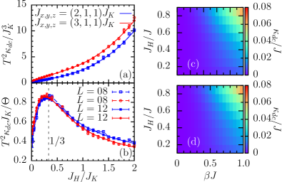
Figure 3: (a) $T^{2}\kappa_{dc}$ and (b) $T^{2}\kappa_{dc}/\Theta$ versus the ratio $J_{H}/J_{K}$ at $\beta=0$ via DQT. Open points correspond to $L=8$ while the filled ones to $L=12$. (c) and (d), heatmap of $\kappa_{dc}$ for $L=10$ versus temperature and the couplings $J_{K}$, $J_{H}$ keeping $J$ fixed. (c) corresponds to $J_{x,y,z}=(2,1,1)J_{K}$ and (d) to $J_{x,y,z}=(3,1,1)J_{K}$.

Let us now focus on the dc part of the thermal transport, both, versus the coupling constants, as well as the temperature and for $J_{x,y,z}/J_{K}=(2,1,1),(3,1,1)$, i.e. for a gapless and a gapped case. We begin with $T^{2}\kappa_{dc}$ versus $J_{K}/J_{H}$ at $\beta=0$ in Fig. 3(a). A clearly monotonous increase with increasing $J_{H}$ is observable, corroborating not only the insulating behavior of the KL, but also a critical coupling for localization of $J_{H}=0$. In fact the data can be fitted very well by a fourth order polynomial with minor offsets, strongly suggesting an insulator as $J_{H}\rightarrow 0$. Next, we normalize to the sum-rule, displaying $T^{2}\kappa_{dc}/\Theta$ in Fig. 3(b). This can be viewed as a rough measure for a zero-frequency current life-time. Once again, this figure shows a clear scale of $J_{H}\approx J_{K}/3$, separating the KL QSL from the HL RSP. The rapid decrease of $\kappa_{dc}/\Theta$ below this scale is dictated by the onset of localization, i.e. the vanishing of $\kappa_{dc}$. This is in sharp contrast to the physics of the HL, where the current life-time at $\beta=0$ is a finite constant. Interestingly the two regimes are connected non-monotonously. It is tempting to speculate that this may imply a reduction of current scattering at the crossover to fractionalization. In passing, Fig. 3(a),(b) prove that finite size effects are negligible, showing little difference between $L=8\mbox{~{}and~{}}12$.

Next, we consider two contour plots of the temperature dependence of $\kappa_{dc}$ versus $J_{H}/J$ at $J_{x,y,z}/J_{K}=(2,1,1)$ and $(3,1,1)$ in Figs. 3(c) and (d). The data is represented keeping the effective energy scale $J$ constant. This figure clearly shows how a low-temperature regime of enhanced dc conductivity developing in the upper right hand corner of the plot, as the system recombines localized Majorana fermions into mobile triplons upon increasing $J_{H}/J$. We note that $\kappa_{dc}\propto\beta^{2}$ as $\beta\rightarrow 0,\forall J_{H}/J$. This leads to the blue regions in Figs. 3(c),(d). The main point relating to the latter is, that for $J_{H}=0$ this region extends over all $\beta$, consistent with an insulator at all temperatures Metavitsiadis and Brenig (2017). Finally, in view of the similar appearance of Figs. 3(c),(d), differences between the gapped and gapless case, which are certainly present for $\beta>1/J$ remain inaccessible to our numerical approach.

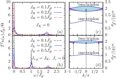
Figure 4: (a) and (b), $T^{2}\kappa(\omega)/\Theta$ versus frequency in the strong-rung limit for Heisenberg $J_{H}/J_{H}^{\prime}=0.1,0.2,0.5$ and Kitaev $J_{K}/J_{H}^{\prime}=0.1,0.2,0.5$ legs respectively obtained via ED at $\beta=0$. (c) and (d), low lying excitation spectrum derived from perturbation theory in the strong-rung limit. The light blue region denotes the two-triplon continuum while the violet dashed lines two-triplon bound states.

Now we change the perspective, and shed light on the impact of Kitaev exchange as a perturbation, starting from the popular strong rung limit of the HL, i.e. for $J_{H}^{\prime}\gg J_{K},J_{H}$. For $J_{K},J_{H}=0$ the ground state $|GS\rangle$ is a RSP state, with energy $E_{GS}/L=-3J_{H}^{\prime}/4$. Finite $J_{K},J_{H}$ both shift $E_{GS}$ and induce dispersive triplon excitations $|k,s\rangle$, with momentum $k$ and magnetization $s$. We evaluate by perturbation theory Papanicolaou and Spathis (1990); Reigrotzki et al. (1994); Kotov et al. (1999) the one and two triplon energies,

$$\frac{\omega^{(1)}(k)}{J_{H}^{\prime}}=1+\lambda\cos k,~{}\frac{\omega^{(2)}(k)}{J_{H}^{\prime}}=2\left(1\pm\lambda\cos\frac{k}{2}\right),$$ (4)

where $\omega^{(2)}(k)$ stands for the boundaries of the two-triplon continuum, while $\lambda=J_{H}/J_{H}^{\prime}$ and $J_{K}/2J_{H}^{\prime}$, for Heisenberg [Fig. 4(c)] and Kitaev [Fig. 4(d)] leg interactions respectively. While these figures include our results for two-triplon bound states, they will not be considered further, since they branch off the continuum only near the zone boundary, and are not expected to contribute significantly to $\kappa(\omega)$ cit .

From Figs. 4(c),(d) and Eq. (4), we can now interpret ED for $\kappa(\omega)$ with $L=8$ at $\beta=0$ for Heisenberg, versus Kitaev legs, in Figs. 4(a) versus (b). In both cases intensity at $\omega\sim 0$ arises from thermally populated triplon states, comprising a Drude weight on finite systems. Additionally however, for Heisenberg legs $j^{\epsilon}|GS\rangle$ generates a state in the two triplon manifold, which combined with the selection rules $\Delta S_{z}=0$ and $\Delta k=0$, dictated by the symmetries of the Heisenberg Hamiltonian, results in transitions with energies $\omega\sim 2J_{H}^{\prime}(1\pm J_{H}/J_{H}^{\prime})$. This is clearly seen in Figs. 4(a). In sharp contrast, Kitaev legs induce an additional current mode at $\omega\sim J_{H}^{\prime}$, visible in Fig. 4(b). This qualitative change is a direct consequence of the loss of $SU(2)$ invariance, which allows for heat-current transitions between one- and two-triplon states, subject to a $\Delta k=0$ only. This one-triplon current intensity will feature a strong temperature dependence $\sim\exp(-J_{H}^{\prime}/T)$ as it involves only excited states. As Figs. 4(a),(b) show our interpretation remains intact up to fairly strong leg couplings $J_{K,H}/J_{H}^{\prime}\approx 0.5$. Finally, we note that $j^{\epsilon}|GS\rangle$ also induces low intensities at three triplon energies, not considered here.

To summarize, we have uncovered several fingerprint of a proximate Kitaev QSL manifested at various energy scales in the dynamical thermal transport of the Kitaev-Heisenberg ladder. While born out of a quasi-1D model study, our results should be transferable to 2D except for the singular behavior at $J_{H}=0$ due to the difference between localization in 1D and 2D. We hope this may stimulate experiments, realizing that not only dc thermal conductivity is a well established experimental probe, but also dynamical heat transport can be addressed, e.g. via fluorescent flash methods Montagnese et al. (2013); Otter et al. (2009) or pump-probe techniques Schmidt et al. (2008). Moreover, a “tuning” of the exchange couplings, discussed here theoretically, is also experimentally feasible - within certain limits - by chemical substitution or external pressure.

References

- Savary and Balents (2017) L. Savary and L. Balents, Reports on Progress in Physics 80, 016502 (2017).
- Zhou et al. (2017) Y. Zhou, K. Kanoda, and T.-K. Ng, Rev. Mod. Phys. 89, 025003 (2017).
- Coldea et al. (2001) R. Coldea, D. A. Tennant, A. M. Tsvelik, and Z. Tylczynski, Phys. Rev. Lett. 86, 1335 (2001).
- Helton et al. (2007) J. S. Helton, K. Matan, M. P. Shores, E. A. Nytko, B. M. Bartlett, Y. Yoshida, Y. Takano, A. Suslov, Y. Qiu, J.-H. Chung, D. G. Nocera, and Y. S. Lee, Phys. Rev. Lett. 98, 107204 (2007).
- Gomilšek et al. (2017) M. Gomilšek, M. Klanjšek, R. Žitko, M. Pregelj, F. Bert, P. Mendels, Y. Li, Q. M. Zhang, and A. Zorko, Phys. Rev. Lett. 119, 137205 (2017).
- Hermanns et al. (2015) M. Hermanns, K. O’Brien, and S. Trebst, Phys. Rev. Lett. 114, 157202 (2015).
- Le Hur et al. (2017) K. Le Hur, A. Soret, and F. Yang, Phys. Rev. B 96, 205109 (2017).
- Lee (2014) P. A. Lee, Journal of Physics: Conference Series 529, 012001 (2014).
- Kitaev (2006) A. Kitaev, Annals of Physics 321, 2 (2006), january Special Issue.
- Hermanns et al. (2018) M. Hermanns, I. Kimchi, and J. Knolle, Annual Review of Condensed Matter Physics 9, 17 (2018).
- Duan et al. (2003) L.-M. Duan, E. Demler, and M. D. Lukin, Phys. Rev. Lett. 91, 090402 (2003).
- Jackeli and Khaliullin (2009) G. Jackeli and G. Khaliullin, Phys. Rev. Lett. 102, 017205 (2009).
- Chaloupka et al. (2010) J. c. v. Chaloupka, G. Jackeli, and G. Khaliullin, Phys. Rev. Lett. 105, 027204 (2010).
- Yadav et al. (2016) R. Yadav, N. A. Bogdanov, V. M. Katukuri, S. Nishimoto, J. van den Brink, and L. Hozoi, Scientific Reports 6, 37925 (2016).
- Choi et al. (2012) S. K. Choi, R. Coldea, A. N. Kolmogorov, T. Lancaster, I. I. Mazin, S. J. Blundell, P. G. Radaelli, Y. Singh, P. Gegenwart, K. R. Choi, S.-W. Cheong, P. J. Baker, C. Stock, and J. Taylor, Phys. Rev. Lett. 108, 127204 (2012).
- Nishimoto et al. (2016) S. Nishimoto, V. M. Katukuri, V. Yushankhai, H. Stoll, U. K. Rößler, L. Hozoi, I. Rousochatzakis, and J. van den Brink, Nature Communications 7, 10273 (2016).
- Ye et al. (2012) F. Ye, S. Chi, H. Cao, B. C. Chakoumakos, J. A. Fernandez-Baca, R. Custelcean, T. F. Qi, O. B. Korneta, and G. Cao, Phys. Rev. B 85, 180403 (2012).
- Kitagawa et al. (2018) K. Kitagawa, T. Takayama, Y. Matsumoto, A. Kato, R. Takano, Y. Kishimoto, S. Bette, R. Dinnebier, G. Jackeli, and H. Takagi, Nature 554, 341 (2018).
- Banerjee et al. (2016) A. Banerjee, C. A. Bridges, J.-Q. Yan, A. A. Aczel, L. Li, M. B. Stone, G. E. Granroth, M. D. Lumsden, Y. Yiu, J. Knolle, S. Bhattacharjee, D. L. Kovrizhin, R. Moessner, D. A. Tennant, D. G. Mandrus, and S. E. Nagler, Nature Materials 15, 733 (2016).
- Sandilands et al. (2015) L. J. Sandilands, Y. Tian, K. W. Plumb, Y.-J. Kim, and K. S. Burch, Phys. Rev. Lett. 114, 147201 (2015).
- Glamazda et al. (2017) A. Glamazda, P. Lemmens, S.-H. Do, Y. S. Kwon, and K.-Y. Choi, Phys. Rev. B 95, 174429 (2017).
- Winter et al. (2018) S. M. Winter, K. Riedl, D. Kaib, R. Coldea, and R. Valentí, Phys. Rev. Lett. 120, 077203 (2018).
- Nasu et al. (2016) J. Nasu, J. Knolle, D. Kovrizhin, Y. Motome, and R. Moessner, Nature Physics 12, 912 (2016).
- Winter et al. (2017) S. M. Winter, K. Riedl, P. A. Maksimov, A. L. Chernyshev, A. Honecker, and R. Valentí, Nature Communications 8, 1152 (2017).
- Hess et al. (2003) C. Hess, B. Büchner, U. Ammerahl, L. Colonescu, F. Heidrich-Meisner, W. Brenig, and A. Revcolevschi, Phys. Rev. Lett. 90, 197002 (2003).
- Hlubek et al. (2010) N. Hlubek, P. Ribeiro, R. Saint-Martin, A. Revcolevschi, G. Roth, G. Behr, B. Büchner, and C. Hess, Phys. Rev. B 81, 020405 (2010).
- Hirobe et al. (2017) D. Hirobe, M. Sato, Y. Shiomi, H. Tanaka, and E. Saitoh, Phys. Rev. B 95, 241112 (2017).
- Yu et al. (2018) Y. J. Yu, Y. Xu, K. J. Ran, J. M. Ni, Y. Y. Huang, J. H. Wang, J. S. Wen, and S. Y. Li, Phys. Rev. Lett. 120, 067202 (2018).
- Hentrich et al. (2018) R. Hentrich, A. U. B. Wolter, X. Zotos, W. Brenig, D. Nowak, A. Isaeva, T. Doert, A. Banerjee, P. Lampen-Kelley, D. G. Mandrus, S. E. Nagler, J. Sears, Y.-J. Kim, B. Büchner, and C. Hess, Phys. Rev. Lett. 120, 117204 (2018).
- Leahy et al. (2017) I. A. Leahy, C. A. Pocs, P. E. Siegfried, D. Graf, S.-H. Do, K.-Y. Choi, B. Normand, and M. Lee, Phys. Rev. Lett. 118, 187203 (2017).
- Hentrich et al. (2018) R. Hentrich, M. Roslova, A. Isaeva, T. Doert, W. Brenig, B. Büchner, and C. Hess, ArXiv e-prints (2018), arXiv:1803.08162 [cond-mat.str-el] .
- Baek et al. (2017) S.-H. Baek, S.-H. Do, K.-Y. Choi, Y. S. Kwon, A. U. B. Wolter, S. Nishimoto, J. van den Brink, and B. Büchner, Phys. Rev. Lett. 119, 037201 (2017).
- Kasahara et al. (2018) Y. Kasahara, T. Ohnishi, Y. Mizukami, O. Tanaka, S. Ma, K. Sugii, N. Kurita, H. Tanaka, J. Nasu, Y. Motome, T. Shibauchi, and Y. Matsuda, ArXiv e-prints (2018), arXiv:1805.05022 [cond-mat.str-el] .
- Nasu et al. (2017) J. Nasu, J. Yoshitake, and Y. Motome, Phys. Rev. Lett. 119, 127204 (2017).
- Metavitsiadis and Brenig (2017) A. Metavitsiadis and W. Brenig, Phys. Rev. B 96, 041115 (2017).
- Metavitsiadis et al. (2017) A. Metavitsiadis, A. Pidatella, and W. Brenig, Phys. Rev. B 96, 205121 (2017).
- Briffa and Zotos (2018) A. K. R. Briffa and X. Zotos, Phys. Rev. B 97, 064406 (2018).
- Stamokostas et al. (2017) G. L. Stamokostas, P. E. Lapas, and G. A. Fiete, Phys. Rev. B 95, 064410 (2017).
- Feng et al. (2007) X.-Y. Feng, G.-M. Zhang, and T. Xiang, Phys. Rev. Lett. 98, 087204 (2007).
- Wu (2012) N. Wu, Physics Letters A 376, 3530 (2012).
- Dagotto and Rice (1996) E. Dagotto and T. M. Rice, Science 271, 618 (1996).
- Zotos (2004) X. Zotos, Phys. Rev. Lett. 92, 067202 (2004).
- Steinigeweg et al. (2016) R. Steinigeweg, J. Herbrych, X. Zotos, and W. Brenig, Phys. Rev. Lett. 116, 017202 (2016).
- Mahan (1981) G. D. Mahan, Many-particle physics (Plenum Press, New York, 1981) pp. xiv, 1003.
- Zotos and Prelovšek (1996) X. Zotos and P. Prelovšek, Phys. Rev. B 53, 983 (1996).
- Steinigeweg et al. (2014) R. Steinigeweg, J. Gemmer, and W. Brenig, Phys. Rev. Lett. 112, 120601 (2014).
- Shastry (2006) B. S. Shastry, Phys. Rev. B 73, 085117 (2006).
- Anderson (1958) P. W. Anderson, Phys. Rev. 109, 1492 (1958).
- Agrapidis et al. (shed) C. E. Agrapidis, J. van den Brink, and S. Nishimoto, (unpublished).
- Papanicolaou and Spathis (1990) N. Papanicolaou and P. Spathis, Journal of Physics: Condensed Matter 2, 6575 (1990).
- Reigrotzki et al. (1994) M. Reigrotzki, H. Tsunetsugu, and T. M. Rice, Journal of Physics: Condensed Matter 6, 9235 (1994).
- Kotov et al. (1999) V. N. Kotov, O. P. Sushkov, and R. Eder, Phys. Rev. B 59, 6266 (1999).
- (53) For more information see supplemental material.
- Montagnese et al. (2013) M. Montagnese, M. Otter, X. Zotos, D. A. Fishman, N. Hlubek, O. Mityashkin, C. Hess, R. Saint-Martin, S. Singh, A. Revcolevschi, and P. H. M. van Loosdrecht, Phys. Rev. Lett. 110, 147206 (2013).
- Otter et al. (2009) M. Otter, V. Krasnikov, D. Fishman, M. Pshenichnikov, R. Saint-Martin, A. Revcolevschi, and P. van Loosdrecht, Journal of Magnetism and Magnetic Materials 321, 796 (2009), proceedings of the Forth Moscow International Symposium on Magnetism.
- Schmidt et al. (2008) A. Schmidt, M. Chiesa, X. Chen, and G. Chen, Review of Scientific Instruments 79, 064902 (2008).