Spatial Frequency Loss for Learning Convolutional Autoencoders

Abstract

This paper presents a learning method for convolutional autoencoders (CAEs) for extracting features from images. CAEs can be obtained by utilizing convolutional neural networks to learn an approximation to the identity function in an unsupervised manner. The loss function based on the pixel loss (PL) that is the mean squared error between the pixel values of original and reconstructed images is the common choice for learning. However, using the loss function leads to blurred reconstructed images. A method for learning CAEs using a loss function computed from features reflecting spatial frequencies is proposed to mitigate the problem. The blurs in reconstructed images show lack of high spatial frequency components mainly constituting edges and detailed textures that are important features for tasks such as object detection and spatial matching. In order to evaluate the lack of components, a convolutional layer with a Laplacian filter bank as weights is added to CAEs and the mean squared error of features in a subband, called the spatial frequency loss (SFL), is computed from the outputs of each filter. The learning is performed using a loss function based on the SFL. Empirical evaluation demonstrates that using the SFL reduces the blurs in reconstructed images.

1 Introduction

Extracting features from images is crucial as a basis for tasks such as object detection and spatial matching. Although there are several feature extraction methods, extracting features using deep learning has attracted much attention. Using deep learning, we can automatically construct a feature extraction algorithm as a mapping represented by a multi-layer neural network. In particular, convolutional neural networks (CNNs)[12] in which filters for convolutional operations are automatically learnt have been widely used. The typical example of using CNNs is category classification for images. CNNs learnt using a large-scale labeled image dataset can extract features from a lot of objects[10, 17]. The features can even be transferred to tasks other than classification. However, annotating a large number of images is time-consuming, thus considering feature extraction based on unsupervised learning is necessary.

A way to realize feature extraction based on unsupervised learning is to use autoencoders[6]. Autoencoders can be obtained by utilizing multi-layer neural networks to learn an approximation to the identity function in an unsupervised manner. Several investigators have shown that the features obtained from hidden layers of autoencoders are useful for the tasks such as image retrieval[9], image classification[11] and image clustering[18]. The architecture of the networks used in [9] and [18] are fully connected, and the network used in [11] has local receptive fields that are not convolutional. Although the networks are reasonable to approximate the identity function, images with the same resolution have to be fed into the networks.

A learning algorithm for convolutional autoencoders (CAEs) for extracting features from images is considered in this paper. In CAEs, the inputs and outputs of CNNs are original and reconstructed images, and the differences between them are tried to minimize to learn an approximation to the identity function. The following advantages are main reasons to choose CAEs:(1) images with arbitrary resolutions can be used both in learning and prediction phases owing to weight sharing, (2) spatial dependency of features can be controlled by changing the resolutions of feature maps in hidden layers, (3) connecting CAEs to other CNNs is easy. Beside these advantages, CAEs have a well-known issue: learning CAEs using the loss function based on the pixel loss (PL) that is the mean squared error between the pixel values of original images and reconstructed images leads to blurred reconstructed images. Since the blurs show lack of information in features extracted in hidden layers to reproduce original images, to address the issue is important for feature extraction.

Another way for feature extraction via unsupervised learning is to use deep convolutional generative adversarial networks (DCGANs)[4, 13, 2, 14]. Two CNNs called a generator and a discriminator are used in DCGANs. Images are generated from random variables in the former, discrimination between generated images and corresponding original images is performed in the latter. The objective of learning DCGANs is to generate images that cannot be discriminated from corresponding original images. It’s shown that the images generated by DCGANs have little blurs. The reduction of blurs comes from the evaluation of generated images not using pixel values but using features utilizing in a discriminator. It confirms that the evaluation using features extracted by networks is useful in image style transfer as well[3, 8].

A way of addressing the issue of CAEs is considered here while keeping the image evaluation using features obtained by networks in mind. The blurs in reconstructed images show lack of high spatial frequency components mainly constituting edges and detailed textures that are important features for tasks such as object detection and spatial matching. That is, learning based on the PL does not exploit the information on high spatial frequency components. In order to exploit the information, a method for learning CAEs using a loss function computed from features reflecting spatial frequencies is proposed. The proposed method extracts features reflecting spatial frequencies from both original and reconstructed images by a Laplacian filter bank that has band-pass property. More precisely, a convolutional layer with a Laplacian filter bank as weights is added to CAEs and the mean squared error of features in a subband, called the spatial frequency loss (SFL), is computed from the outputs of each filter. Since we can separate features with high spatial frequencies from features with low spatial frequencies by a Laplacian filter bank, the learning algorithm based on the SFL exploits the information on high spatial frequency components to reproduce original images.

The differences between the proposed method and DCGANs are twofold: (1) The evaluation of images in DCGANs is performed using features obtained by a discriminator. In this case, the information reflected by the features is determined by an image dataset used in learning. Thus it’s not ambiguous that the features have the information on specific spatial frequencies. On the other hand, the proposed method uses the features explicitly reflecting specific spatial frequencies to evaluate images. (2) Since only a single layer has to be added to CAEs to extract the features by a Laplacian filter bank, the additional computational costs in learning is quite small compared to DCGANs. As demonstrated in the experimental results, introducing the features reflecting specific spatial frequencies is clearly effective to reduce the blurs in reconstructed images.

This paper organized as follows: Section 2 explains CAEs. The learning method using the loss function based on the SFL is proposed in Sec.3. The experimental results are shown in Sec.4. Section 5 summarizes this paper.

2 Convolutional Autoencoders (CAEs)

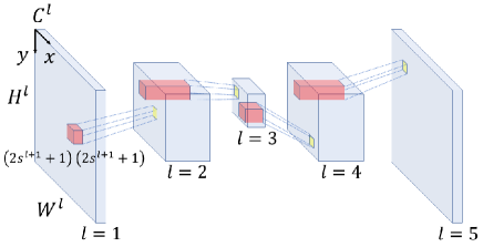
Figure 1: An example of a CAE. The number of layer $L$ is five. A mapping between the input layer and the output layer is realized by applying the filters with the size $C^{l+1}\left(2s^{l+1}+1\right)\left(2s^{l+1}+1\right)$ to the volume data with the size $C^{l}W^{l}H^{l}$. The output layer has feature maps with the same size as an original image and learning is performed to reproduce the original image in the feature maps.

A fully convolutional network[7, 16] is used to constitute a CAE in this paper. It assumes that a $L$ layer CNN such as Fig.1 has the volume data with the number of channels $C^{l}$, width $W^{l}$ and height $H^{l}$, $l=1,\ldots,L$. The volume data are represented as follows:

$$f^{l}\left(c,x,y\right),$$ (1)

$$c=1,\ldots,C^{l},~{}x=1,\ldots,W^{l},~{}y=1,\ldots,H^{l}.$$

The voxels in $f^{l}\left(c,x,y\right)$ correspond to artificial neurons. The volume data in the $\left(l+1\right)$-th layer are computed from one in the $l$-th layer using convolution operations and an activation function as follows:

$$o^{l+1}\left(c,x,y\right)=\sum_{c^{\prime}=1}^{C^{l}}\cdot$$

$$\sum_{\alpha=-s^{l+1}}^{s^{l+1}}\sum_{\beta=-s^{l+1}}^{s^{l+1}}f^{l}\left(c^{\prime},x+\alpha,y+\beta\right)w^{l+1}(c,c^{\prime},\alpha,\beta)$$ (2)

$$f^{l+1}\left(c,x,y\right)=a^{l+1}\left(o^{l+1}\left(c,x,y\right)+b^{l+1}\left(c\right)\right)$$ (3)

where, $w^{l+1}(c,c^{\prime},\alpha,\beta)$, $c=1,\ldots,C^{l+1}$ are filters with the size $C^{l+1}\left(2s^{l+1}+1\right)\left(2s^{l+1}+1\right)$, $s^{l+1}\in\mathcal{N}$, $b^{l+1}\left(c\right)$ are biases and $a^{l+1}\left(\cdot\right)$ is an activation function. The variables $\alpha$ and $\beta$ denote the horizontal and vertical shifts from $\left(x,y\right)$ and their origin is the center of a filter. Since the equations (2) and (3) can be regarded as feature extraction by convolution operations, $f^{l}\left(c,x,y\right)$, $l>1$ are called feature maps.

The input layer of a CAE is an original image and the output layer has feature maps with the same size as an original image. The filters and biases of a CAE are adjusted by learning so as to reproduce the original image in the feature maps of the output layer. A five layer CAE is shown in Fig.1 as an example.

The number of channels of hidden layers of CAEs should be smaller than the total number of channels of original images in an image dataset used in learning so that CAEs tries to reconstruct original images from the restricted features appeared in hidden layers. It turns out to extract common and useful features from original images to reconstruct them. Since no annotating images is required, the feature extraction by CAEs is realized by unsupervised learning.

3 Learning CAEs Using Spatial Frequency Loss

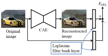
Figure 2: An example of the network for learning a CAE using the loss function $E_{SFL}$ based on the proposed spatial frequency loss. A convolutional layer with the weights obtained from a Laplacian filter bank is added to the CAE. The loss function $E_{SFL}$ is computed by inputting original and reconstructed images to the Laplacian filter bank layer to extract features reflecting spatial frequencies.

This section proposes a novel loss function for learning CAEs. We can use any loss functions that are consistent with the purpose of reconstructing original images. One of the loss functions is the following $E_{PL}$ based on the PL that is the mean squared error between the pixel values of original and reconstructed images:

$$E_{PL}=\frac{1}{N}\sum_{i=1}^{N}\sum_{c=1}^{c^{L}}w_{PL}\left(c\right)E_{PL}^{L}\left(i,c\right)$$ (4)

$$E_{PL}^{L}\left(i,c\right)=\frac{1}{2}\frac{1}{W^{L}H^{L}}\cdot$$

$$\hskip 8.5359pt\sum_{x=1}^{W^{L}}\sum_{y=1}^{H^{L}}\left\{f_{i}^{L}\left(c,x,y\right)-f_{i}^{1}\left(c,x,y\right)\right\}^{2}$$

where, $N$ is the number of images in a dataset, $w_{PL}\left(c\right)$ are the weights for the channels in the $L$-th layer and the subscript $i$ for the volume data represents the $i$-th image in a dataset. Although $E_{PL}$ is straightforward for the purposed of CAEs, learning using $E_{PL}$ leads to blurred reconstructed images, which show lack of high spatial frequency components.

High spatial frequency components mainly constitute edges and detailed textures that are important features for tasks such as object detection and spatial matching. Thus generating more clear reconstructed images by compensating the lack of components is important for feature extraction. In order to generate more clear reconstructed images, a learning method for CAEs using a loss function computed from features reflecting spatial frequencies is proposed. In the proposed method, a convolutional layer with a Laplacian filter back as weights is added to CAEs, and the loss function is computed from the outputs of the layer. Figure 2 shows an example of the network for learning a CAE using the proposed loss function.

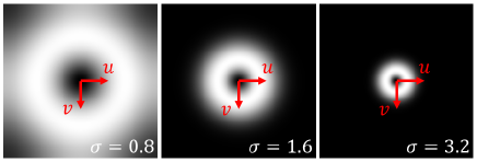
Figure 3: The frequency responses of the Laplacian filters with the scales $\sigma=0.8,~{}1.6$ and $3.2$. The $u$ and $v$ in these figures represent the spatial frequencies for $x$ and $y$ directions, respectively. The brightness of the images show the power spectra. As we can see from the figures, the Laplacian filter has band-pass property.

The Laplacian filter has the coefficients obtained from the following normalized Laplacian of Gaussian function:

$$\sigma^{2}\nabla^{2}g\left(x,y\right)=-\left(2-\frac{x^{2}+y^{2}}{\sigma^{2}}\right)g\left(x,y\right)$$ (5)

$$g\left(x,y\right)=\frac{1}{2\pi\sigma^{2}}e^{-\frac{x^{2}+y^{2}}{2\sigma^{2}}}$$

where, $\sigma$ is the scale. Figure 3 shows the frequency responses of the Laplacian filters with the scales $\sigma=0.8,1.6$ and $3.2$. As we can see from these figures, the Laplacian filter has band-pass property. The subband passed by the filter varies with the scale; the smaller scale is used, the higher spatial frequency is passed. Thus using the Laplacian filter bank, we can extract features in each subband from original and reconstructed images. Figure 4 represents an example of the outputs of the Laplacian filter bank. The outputs reflect the spatial frequencies because the smaller scale is used, the smaller changes in brightness are extracted.

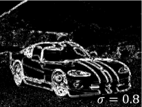
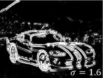
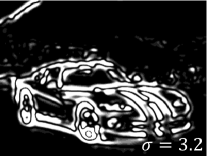
Figure 4: An example of the outputs of the Laplacian filter bank. The outputs are squared and quantized to the uniform 10 levels in [0:255]. The outputs reflect the spatial frequencies because the smaller scale is used, the smaller changes in brightness are extracted.

The definition of the spatial frequency loss (SFL) is now shown. Let a convolutional layer added to CAEs be the $\left(L+1\right)$-th layer. The activation function of the $\left(L+1\right)$-th layer is the identity function and the biases are 0. The SFL denoted by $E_{SFL}^{L+1}$ is defined by the mean squared error of features in a subband computed from the outputs of the $\left(L+1\right)$-th layer, and the loss function $E_{SFL}$ is constructed from the SFL as follows:

$$E_{SFL}=\frac{1}{N}\sum_{i=1}^{N}\sum_{c=1}^{C^{L+1}}w_{SFL}\left(c\right)E_{SFL}^{L+1}\left(i,c\left|\sigma_{c}\right.\right)$$ (6)

$$E_{SFL}^{L+1}\left(i,c\left|\sigma_{c}\right.\right)=\frac{1}{2}\frac{1}{W^{L+1}H^{L+1}}\cdot$$

$$\hskip 2.84544pt\sum_{x=1}^{W^{L+1}}\sum_{y=1}^{H^{L+1}}\left\{f_{i}^{L+1}\left(c,x,y\left|\sigma_{c}\right.\right)-f_{i}^{1}\left(c,x,y\left|\sigma_{c}\right.\right)\right\}^{2}$$

where, $w_{SFL}\left(c\right)$ are the weights for subbands and $f_{i}^{L+1}\left(c,x,y\left|\sigma_{c}\right.\right)$ and $f_{i}^{1}\left(c,x,y\left|\sigma_{c}\right.\right)$ are the results of applying the Laplacian filter with the scales $\sigma_{c}$ to reconstructed and original images, respectively. The number of channels $C^{L+1}$ is determined by the number of filters in a Laplacian filter bank.

We can evaluate the losses of subbands by $E_{SFL}$. However, the losses of whole spatial frequencies can not be computed due to the band-pass property of the Laplacian filter. Therefore, the following loss function $E$ is used for learning CAEs, so that the losses of whole spatial frequencies are evaluated by $E_{PL}$.

$$E=E_{PL}+E_{SFL}$$ (7)

The backpropagation algorithm[15] is applied to learning CAEs with the loss function of Eq.(7). First, the following gradients of the $E_{SFL}$ with respect to the outputs of the $\left(L+1\right)$-th layer are computed in learning:

$$\frac{\partial E_{SFL}}{\partial o_{i}^{L+1}\left(c,x,y\left|\sigma_{c}\right.\right)}=\frac{1}{N_{m}}\sum_{i=1}^{N_{m}}\biggl{[}w_{SFL}\left(c\right)\cdot$$ (8)

$$\left.\frac{1}{W^{L+1}H^{L+1}}\left\{f_{i}^{L+1}\left(c,x,y\left|\sigma_{c}\right.\right)-f_{i}^{1}\left(c,x,y\left|\sigma_{c}\right.\right)\right\}\right]$$

where, $N_{m}$ is the number of images in a mini-batch and $o_{i}^{L+1}\left(c,x,y\left|\sigma_{c}\right.\right)$ are the outputs of the $\left(L+1\right)$-th layer obtained by Eq.(2) for the $i$-th image in a mini-batch. The gradients are backpropagated to the $L$-th layer. Then, the following gradients of $E_{PL}$ are computed at the $L$-th layer:

$$\frac{\partial E_{PL}}{\partial o_{i}^{L}\left(c,x,y\right)}=\frac{1}{N_{m}}\sum_{i=1}^{N_{m}}\biggl{[}w_{PL}\left(c\right)\cdot$$ (9)

$$\left.\frac{1}{W^{L}H^{L}}\left\{f_{i}^{L}\left(c,x,y\right)-f_{i}^{1}\left(c,x,y\right)\right\}\cdot\frac{\partial f_{i}^{L}\left(c,x,y\right)}{\partial o_{i}^{L}\left(c,x,y\right)}\right]$$

where, $\frac{\partial f_{i}^{L}\left(c,x,y\right)}{\partial o_{i}^{L}\left(c,x,y\right)}$ are derived from the activation function $a^{L}\left(\cdot\right)$. The gradients of Eq.(9) are added to the gradients backpropagated from the $\left(L+1\right)$-th layer, followed by backpropagating the results to hidden layers of CAEs to adjust filters and biases. The learning algorithm taking both the PL and SFL into account is performed in this way.

4 Experimental Results

Table 1: The architecture of the CNN for learning. From the first to the fifth layers constituted a CAE. The sixth layer had the weights obtained from the Laplacian filter bank in which three filters were used.

Layer	Filter	Stride	Activation
no.	size		function
1	n/a	n/a	n/a
2	$32\times 3\times 3$	1	ReLU
3	$16\times 3\times 3$	2	ReLU
4	$32\times 3\times 3$	0.5	ReLU
5	$3\times 3\times 3$	1	$\tanh$
6	$3\times\lceil 8\sigma_{c}\rceil\times\lceil 8\sigma_{c}\rceil$	1	identity

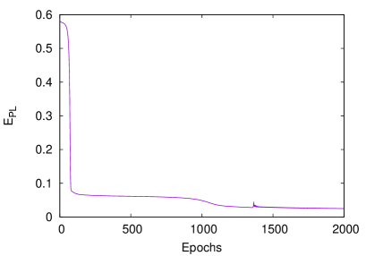
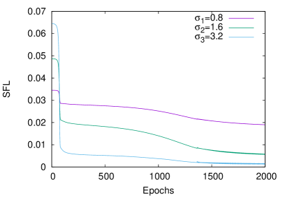
(a)                                                               (b)

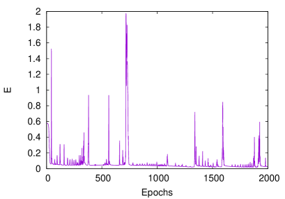
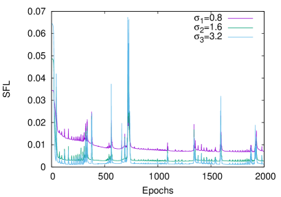
(c)                                                               (d)

Figure 5: Learning curves. (a) The learning using $E_{PL}$. (b) The changes in the SFLs of the subbands in learning of (a). (c) The learning introducing $E_{SFL}$. (d) The changes in the SFLs of the subbands in learning of (c). In (c) and (d), the curves were drawn under the condition of $W_{SFL}\left(c\right)=1$ to make comparison with (a) and (b) easy. In learning using $E_{PL}$, the SFLs of the subbands with $\sigma_{c}=0.8$ and $1.6$ largely remained even though $E_{PL}$ became small. On the other hand, the SFLs were reduced by introducing $E_{SFL}$.

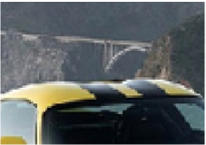
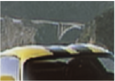
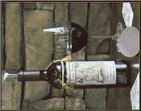
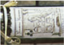
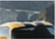
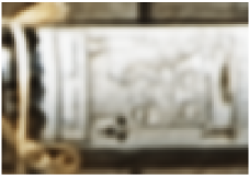
(a)                                                                      (b)

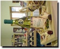
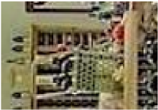
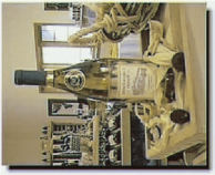
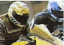
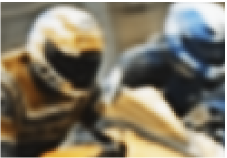
(c)                                                                      (d)

Figure 6: The original images and their reconstruction results. Top row: The original images and close-up of their portion. Middle row: The reconstructed images by the proposed method. Bottom row: The reconstructed images by learning using $E_{PL}$. Introducing $E_{SFL}$ into learning is clearly effective to reduce the blurs.

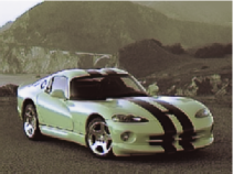
(a)

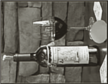
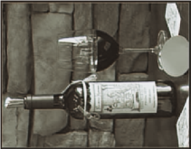
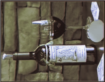
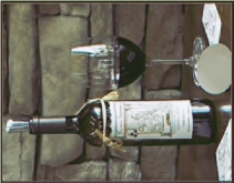
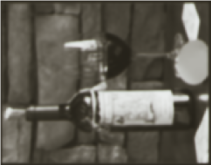
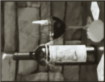
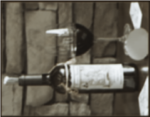
(b)

Figure 7: The reconstructed images for the images in Fig.6(a) and (b) at 100, 500, 1000 and 1500 epochs. Top row: The reconstructed images by the proposed method. Bottom row: The reconstructed images by learning using $E_{PL}$.

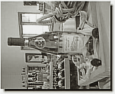
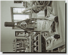
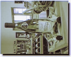
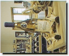
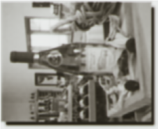
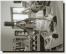
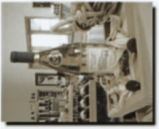
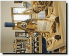
(c)

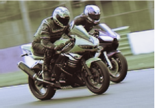
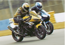
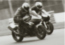
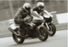
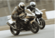
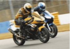
(d)

Figure 7: (continued) The reconstructed images for the images in Fig.6(c) and (d) at 100, 500, 1000 and 1500 epochs. Top row: The reconstructed images by the proposed method. Bottom row: The reconstructed images by learning using $E_{PL}$.

The experiments using the 70 color images in the Proposal Flow Willow dataset[5] were performed to demonstrate the usefulness of the proposed method. The size of the larger side of the original images was equal to 300 pixels and the sizes of the other sides were determined by the aspect ratios.

The architecture of the CNN for learning is shown in Tab.1. From the first layer to the fifth layer constituted a CAE. Since the activation function of the fifth layer was $\tanh$, the pixel values of the original images were scaled to $\left[-1,1\right]$. The resolution of the feature maps of the third layer was the half of the resolution of the original images, because the stride of the third layer was 2. The stride of the fourth layer was 0.5 that means upsampling carried out by the bilinear interpolation[16]. The sixth layer had the weights obtained from the Laplacian filter bank. Since the three filters with the scales $\sigma_{c}=0.8,1.6$ and $3.2$ were used for the filter bank, the sixth layer had the three channels corresponding to the subbands. Although the size of the Laplacian filter was basically decided by $\lceil 8\sigma_{c}\rceil$, the size was changed to an odd number by adding 1 if $\lceil 8\sigma_{c}\rceil$ was an even number.

The backpropagation algorithm with the momentum term[15] was use for learning. The learning coefficient was 0.02 and the weight for the momentum term was 0.5. The initial values of the filters were random numbers given by the distribution $N\left(0,0.02\right)$ and all the initial values of the biases were 0. All the weights $w_{PL}\left(c\right)$ in Eq.(4) were 1. The weights of Eq.(6) were 100 for $\sigma_{c}=0.8$ and 10 for both $\sigma_{c}=1.6$ and $3.2$, which emphasized the loss of the highest subband. The gradients of Eq.(8) and (9) were computed by the full-batch $\left(N_{m}=70\right)$. The maximum epoch was 2000.

The learning algorithm was implemented by C++ and CUDA[1] and performed on both the CPU and the GPU, Intel Xeon E5-2637v4 and NVIDIA Quadro M4000. The computational time for an epoch was about 218 and 214 seconds for the proposed method and the learning using $E_{PL}$, respectively. Thus learning for 2000 epochs required about 5 days.

Figure 5 shows the learning curves. The curve in Fig.5(a) is for learning using $E_{PL}$. The curves in Fig.5(b) represent the changes in the SFLs of the subbands in learning of (a). Note that the gradients of Eq.(8) were not backpropagated in Fig.5(b). As we can see from these figures, the SFLs of the subbands with $\sigma_{c}=0.8$ and $1.6$ largely remained even though $E_{PL}$ became small. In general, the power spectra of images concentrate in low spatial frequencies. Thus reducing the loss of the lowest subband was good way to reproduce the original images and $E_{PL}$ was actually reduced quickly at the beginning of learning. However, reducing the loss of the lowest subband turned out to reduce the gradients of $E_{PL}$ and make the SFLs of the other subbands, especially the SFL of the highest subband, remain. This is the reason why the reconstructed images obtained by learning using $E_{PL}$ have blurs.

Figure 5(c) and (d) represent the learning curves of the proposed method and the changes in the SFLs of the subbands in learning of (c), respectively. Since there is one-to-many uncertainty between the output of the Laplacian filter and the reconstructed image, the network parameters reducing $E_{SFL}$ might increase $E_{PL}$. Therefore, the losses in Fig.5(c) and (d) were oscillated because the network parameters consistent with both $E_{SFL}$ and $E_{PL}$ had to be found out. However, the SFLs of all the subbands were reduced as learning progressed as demonstrated in Fig.5(d). The SFLs of the subbands at 2000 epochs were (18.9,5.69,1.37) ($\times 10^{-3}$) in learning using $E_{PL}$ and (7.08,2.65,1.34) ($\times 10^{-3}$) in the proposed method, in which the SFLs are ordered with decreasing spatial frequencies. These results quantitatively show the usefulness of the proposed method to reduce the SFLs of the high spatial frequency components. Figure 6 represents the reconstructed images for the four original images at 2000 epochs, which were generated by the proposed method and learning using $E_{PL}$. Figure 7 shows the process of reconstruction for the images in Fig.6 at 100, 500, 1000 and 1500 epochs. The reconstructed images in these figures qualitatively demonstrate that the blurs were clearly reduced by the proposed method.

The proposed method extracts the features in subbands by a Laplacian filter bank. By this process, we can separate the features with high spatial frequencies from the features with low spatial frequencies. This separation enables us to perform weighting for the gradients of the subbands by $w_{SFL}\left(c\right)$ in Eq.(8) and facilitate the reconstruction of the features with high spatial frequencies. The key to reducing blurs is the separation of features.

As we can see from Fig.7, both the proposed method and learning using $E_{PL}$ required a large number of epochs to reproduce the colors, although the shapes were reconstructed in the early stage of learning. In addition, a part of the colors did not recall at 2000 epochs as shown in Fig.6. Reproducing correct colors in a short learning time is a problem for future work.

5 Summary

In this paper, the learning method for CAEs using the loss function computed from features reflecting spatial frequencies has been presented to reduce the blurs in reconstructed images. The spatial frequency loss (SFL) was defined using the features extracted by a Laplacian filter bank and the learning algorithm using the loss function constructed from the SFLs was shown. The experimental results were given to demonstrate the usefulness of the proposed method quantitatively and qualitatively. These results will contribute to facilitate the use of CAEs for feature extraction.

References

- [1] CUDA Zone. https://developer.nvidia.com/cuda-zone.
- [2] E. Denton, S. Chintala, A. Szlam, and R. Fergus. Deep generative image models using a Laplacian pyramid of adversarial networks. Advances in Neural Information Processing Systems, 2015.
- [3] L. A. Gatys, A. S. Echker, and M. Bethge. Image style transfer using convolutional neural networks. In Proc. Conf. Computer Vision and Pattern Recognition, 2016.
- [4] I. J. Goodfellow, J. Pouget-Abadie, M. Mirza, B. Xu, D. Warde-Farley, S. Ozair, A. Courville, and Y. Bengio. Generative adversarial nets. Advances in Neural Information Processing Systems, 2014.
- [5] B. Ham, M. Cho, C. Schmid, and J. Ponce. Proposal Flow: semantic correspondences from object proposals. In Proc. Int. Conf. Computer Vision and Pattern Recognition, 2016.
- [6] G. E. Hinton and R. R. Salakhutdinov. Reducing the dimensionality of data with neural networks. SCIENCE, 313:504–507, 2006.
- [7] A. D. J. T. Springenberg, T. Brox, and M. Riedmiller. Striving for simplicity: the all convolutional net. In Proc. Int. Conf. Machine Learning, 2015.
- [8] J. Johnson, A. Alahi, and L. Fei-Fei. Perceptual losses for real-time style transfer and super-resolution. In Proc. European Conf. Computer Vision, 2016.
- [9] A. Krizhevsky and G. E. Hinton. Using very deep autoencoders for content-based image retrieval. In Proc. European Symp. Artificial Neural Networks, 2011.
- [10] A. Krizhevsky, I. Sutskever, and G. E. Hinton. ImageNet classification with deep convolutional neural networks. In Proc. Int. Conf. Neural Information Processing Systems, volume 1, pages 1097–1105, 2012.
- [11] Q. V. Le, M. Ranzato, R. Monga, M. Devin, K. Chen, G. S. Corrado, J. Dean, and A. Y. Ng. Building high-level features using large scale unsupervised learning. In Proc. Int. Conf. Machine Learning, 2012.
- [12] Y. LeCun, O. Matan, B. Boser, J. S. Denker, D. Henderson, R. E. Howard, W. Hubbard, L. D. Jackel, and H. S. Baird. Handwritten zip code recognition with multilayer networks. In Proc. Int. Conf. Pattern Recognition, volume 2, pages 35–40, 1990.
- [13] A. Makhzani, J. Shlens, N. Jaitly, I. Goodfellow, and B. Grey. Adversarial autoencoders. In Proc. Int. Conf. Learning Representation, 2016.
- [14] A. Radford, L. Metz, and S. Chintala. Unsupervised representation learning with deep convolutional generative adversarial networks. In Proc. Int. Conf. Machine Learning, 2016.
- [15] D. E. Rumelhart, G. E. Hinton, and R. J. Williams. Learning representations by back-propagating errors. NATURE, 323(9):533–536, 1986.
- [16] E. Shelhamer, J. Long, and T. Darrell. Fully convolutional networks for semantic segmentation. IEEE Trans. PAMI, 39(4):604–651, 2017.
- [17] K. Simonyan and A. Zisserman. Very deep convolutional networks for large-scale image recognition. In Proc. Int. Conf. Learning Representation, 2015.
- [18] J. Xie, R. Girshick, and A. Farhadi. Unsupervised deep embedding for clustering analysis. In Proc. Int. Conf. Machine Learning, 2016.