Adversarial Regression with Multiple Learners

Abstract

Despite the considerable success enjoyed by machine learning techniques in practice, numerous studies demonstrated that many approaches are vulnerable to attacks. An important class of such attacks involves adversaries changing features at test time to cause incorrect predictions. Previous investigations of this problem pit a single learner against an adversary. However, in many situations an adversary’s decision is aimed at a collection of learners, rather than specifically targeted at each independently. We study the problem of adversarial linear regression with multiple learners. We approximate the resulting game by exhibiting an upper bound on learner loss functions, and show that the resulting game has a unique symmetric equilibrium. We present an algorithm for computing this equilibrium, and show through extensive experiments that equilibrium models are significantly more robust than conventional regularized linear regression.

1 Introduction

Increasing use of machine learning in adversarial settings has motivated a series of efforts investigating the extent to which learning approaches can be subverted by malicious parties. An important class of such attacks involves adversaries changing their behaviors, or features of the environment, to effect an incorrect prediction. Most previous efforts study this problem as an interaction between a single learner and a single attacker (Brückner & Scheffer, 2011; Dalvi et al., 2004; Li & Vorobeychik, 2014; Zhou et al., 2012). However, in reality attackers often target a broad array of potential victim organizations. For example, they craft generic spam templates and generic malware, and then disseminate these widely to maximize impact. The resulting ecology of attack targets reflects not a single learner, but many such learners, all making autonomous decisions about how to detect malicious content, although these decisions often rely on similar training datasets.

We model the resulting game as an interaction between multiple learners, who simultaneously learn linear regression models, and an attacker, who observes the learned models (as in white-box attacks (Šrndic & Laskov, 2014)), and modifies the original feature vectors at test time in order to induce incorrect predictions. Crucially, rather than customizing the attack to each learner (as in typical models), the attacker chooses a single attack for all learners. We term the resulting game a Multi-Learner Stackelberg Game, to allude to its two stages, with learners jointly acting as Stackelberg leaders, and the attacker being the follower. Our first contribution is the formal model of this game. Our second contribution is to approximate this game by deriving upper bounds on the learner loss functions. The resulting approximation yields a game in which there always exists a symmetric equilibrium, and this equilibrium is unique. In addition, we prove that this unique equilibrium can be computed by solving a convex optimization problem. Our third contribution is to show that the equilibrium of the approximate game is robust, both theoretically (by showing it to be equivalent to a particular robust optimization problem), and through extensive experiments, which demonstrate it to be much more robust to attacks than standard regularization approaches.

Related Work Both attacks on and defenses of machine learning approaches have been studied within the literature on adversarial machine learning (Brückner & Scheffer, 2011; Dalvi et al., 2004; Li & Vorobeychik, 2014; Zhou et al., 2012; Lowd & Meek, 2005). These approaches commonly assume a single learner, and consider either the problem of finding evasions against a fixed model (Dalvi et al., 2004; Lowd & Meek, 2005; Šrndic & Laskov, 2014), or algorithmic approaches for making learning more robust to attacks (Russu et al., 2016; Brückner & Scheffer, 2011; Dalvi et al., 2004; Li & Vorobeychik, 2014, 2015). Most of these efforts deal specifically with classification learning, but several consider adversarial tampering with regression models (Alfeld et al., 2016; Grosshans et al., 2013), although still within a single-learner and single-attacker framework. Stevens & Lowd (2013) study the algorithmic problem of attacking multiple linear classifiers, but did not consider the associated game among classifiers.

Our work also has a connection to the literature on security games with multiple defenders (Laszka et al., 2016; Smith et al., 2017; Vorobeychik et al., 2011). The key distinction with our paper is that in multi-learner games, the learner strategy space is the space of possible models in a given model class, whereas prior research has focused on significantly simpler strategies (such as protecting a finite collection of attack targets).

2 Model

We investigate the interactions between a collection of learners $\mathcal{N}=\{1,2,...,n\}$ and an attacker in regression problems, modeled as a Multi-Learner Stackelberg Game (MLSG). At the high level, this game involves two stages: first, all learners choose (train) their models from data, and second, the attacker transforms test data (such as features of the environment, at prediction time) to achieve malicious goals. Below, we first formalize the model of the learners and the attacker, and then formally describe the full game.

2.1 Modeling the Players

At training time, a set of training data $(\mathbf{X},\mathbf{y})$ is drawn from an unknown distribution $\mathcal{D}$. $\mathbf{X}\in\mathbb{R}^{m\times d}$ is the training sample and $\mathbf{y}\in\mathbb{R}^{m\times 1}$ is a vector of values of each data in $\mathbf{X}$. We let $\mathbf{x}_{j}\in\mathbb{R}^{d\times 1}$ denote the $j$th instance in the training sample, associated with a corresponding value $y_{j}\in\mathbb{R}$ from $\mathbf{y}$. Hence, $\mathbf{X}=[\mathbf{x}_{1},...,\mathbf{x}_{m}]^{\top}$ and $\mathbf{y}=[y_{1},y_{2},...,y_{m}]^{\top}$. On the other hand, test data can be generated either from $\mathcal{D}$, the same distribution as the training data, or from $\mathcal{D}^{{}^{\prime}}$, a modification of $\mathcal{D}$ generated by an attacker. The nature of such malicious modifications is described below. We let $\beta\ (0\leq\beta\leq 1)$ represent the probability that a test instance is drawn from $\mathcal{D}^{{}^{\prime}}$ (i.e., the malicious distribution), and $1-\beta$ be the probability that it is generated from $\mathcal{D}$.

The action of the $i$th learner is to select a $d\times 1$ vector $\bm{\theta}_{i}$ as the parameter of the linear regression function $\hat{\mathbf{y}}_{i}=\mathbf{X}\bm{\theta}_{i}$, where $\hat{\mathbf{y}}_{i}$ is the predicted values for data $\mathbf{X}$. The expected cost function of the $i$th learner at test time is then

$$c_{i}(\bm{\theta}_{i},\mathcal{D}^{{}^{\prime}})=\beta\mathbb{E}_{(\mathbf{X}^{{}^{\prime}},\mathbf{y})\sim\mathcal{D}^{{}^{\prime}}}[\ell(\mathbf{X}^{{}^{\prime}}\bm{\theta}_{i},\mathbf{y})]+(1-\beta)\mathbb{E}_{(\mathbf{X},\mathbf{y})\sim\mathcal{D}}[\ell(\mathbf{X}\bm{\theta}_{i},\mathbf{y})].$$ (1)

where $\ell(\hat{\mathbf{y}},\mathbf{y})=||\hat{\mathbf{y}}-\mathbf{y}||_{2}^{2}$. That is, the cost function of a learner $i$ is a combination of its expected cost from both the attacker and the honest source.

Every instance $(\mathbf{x},y)$ generated according to $\mathcal{D}$ is, with probability $\beta$, maliciously modified by the attacker into another, $(\mathbf{x}^{\prime},y)$, as follows. We assume that the attacker has an instance-specific target $z(\mathbf{x})$, and wishes that the prediction made by each learner $i$ on the modified instance, $\hat{y}=\bm{\theta}_{i}^{\top}\mathbf{x}^{{}^{\prime}}$, is close to this target. We measure this objective for the attacker by $\ell(\hat{\mathbf{y}}^{\prime},\mathbf{z})=||\hat{\mathbf{y}}^{\prime}-\mathbf{z}||_{2}^{2}$ for a vector of predicted and target values $\hat{\mathbf{y}}^{\prime}$ and $\hat{\mathbf{z}}$, respectively. In addition, the attacker incurs a cost of transforming a distribution $\mathcal{D}$ into $\mathcal{D}^{{}^{\prime}}$, denoted by $R(\mathcal{D}^{{}^{\prime}},\mathcal{D})$.

After a dataset $(\mathbf{X}^{{}^{\prime}},\mathbf{y})$ is generated in this way by the attacker, it is used simultaneously against all the learners. This is natural in most real attacks: for example, spam templates are commonly generated to be used broadly, against many individuals and organizations, and, similarly, malware executables are often produced to be generally effective, rather than custom made for each target. The expected cost function of the attacker is then a sum of its total expected cost for all learners plus the cost of transforming $\mathcal{D}$ into $\mathcal{D}^{{}^{\prime}}$ with coefficient $\lambda>0$:

$$c_{a}(\{\bm{\theta}_{i}\}_{i=1}^{n},\mathcal{D}^{{}^{\prime}})=\sum_{i=1}^{n}\mathbb{E}_{(\mathbf{X}^{{}^{\prime}},\mathbf{y})\sim\mathcal{D}^{{}^{\prime}}}[\ell(\mathbf{X}^{{}^{\prime}}\bm{\theta}_{i},\mathbf{z})]+\lambda R(\mathcal{D}^{{}^{\prime}},\mathcal{D}).$$ (2)

As is typical, we estimate the cost functions of the learners and the attacker using training data $(\mathbf{X},\mathbf{y})$, which is also used to simulate attacks. Consequently, the cost functions of each learner and the attacker are estimated by

$$c_{i}(\bm{\theta}_{i},\mathbf{X}^{{}^{\prime}})=\beta\ell(\mathbf{X}^{{}^{\prime}}\bm{\theta}_{i},\mathbf{y})+(1-\beta)\ell(\mathbf{X}\bm{\theta}_{i},\mathbf{y})$$ (3)

and

$$c_{a}(\{\bm{\theta}_{i}\}_{i=1}^{n},\mathbf{X}^{{}^{\prime}})=\sum_{i=1}^{n}\ell(\mathbf{X}^{{}^{\prime}}\bm{\theta}_{i},\mathbf{z})+\lambda R(\mathbf{X}^{{}^{\prime}},\mathbf{X})$$ (4)

where the attacker’s modification cost is measured by $R(\mathbf{X}^{{}^{\prime}},\mathbf{X})=||\mathbf{X}^{{}^{\prime}}-\mathbf{X}||_{F}^{2}$, the squared Frobenius norm.

2.2 The Multi-Learner Stackerlberg Game

We are now ready to formally define the game between the $n$ learners and the attacker. The MLSG has two stages: in the first stage, learners simultaneously select their model parameters $\bm{\theta}_{i}$, and in the second stage, the attacker makes its decision (manipulating $\mathbf{X}^{{}^{\prime}}$) after observing the learners’ model choices $\{\bm{\theta}\}_{i=1}^{n}$. We assume that the proposed game satisfies the following assumptions:

1. Players have complete information about parameters $\beta$ (common to all learners) and $\lambda$. This is a strong assumption, and we relax it in our experimental evaluation (Section 6), providing guidance on how to deal with uncertainty about these parameters.

2. Each learner has the same action (model parameter) space $\bm{\Theta}\subseteq\mathbb{R}^{d\times 1}$ which is nonempty, compact and convex. The action space of the attacker is $\mathbb{R}^{m\times d}$.

3. The columns of the training data $\mathbf{X}$ are linearly independent.

We use Multi-Learner Stackelberg Equilibrium (MLSE) as the solution for the MLSG, defined as follows.

Definition 1 (Multi-Learner Stackelberg Equilibrium (MLSE)).

An action profile $(\{\bm{\theta}_{i}^{*}\}_{i=1}^{n},\mathbf{X}^{*})$ is an MLSE if it satisfies

$$\begin{split}\bm{\theta}_{i}^{*}&=\operatorname*{arg\,min}_{\bm{\theta}_{i}\in\bm{\Theta}}c_{i}(\bm{\theta}_{i},\mathbf{X}^{*}(\bm{\theta})),\forall i\in\mathcal{N}\\ &\texttt{s.t. }\mathbf{X}^{*}(\bm{\theta})=\operatorname*{arg\,min}_{\mathbf{X}^{{}^{\prime}}\in\mathbb{R}^{m\times d}}c_{a}(\{\bm{\theta}_{i}\}_{i=1}^{n},\mathbf{X}^{{}^{\prime}}).\end{split}$$ (5)

where $\bm{\theta}=\{\bm{\theta}_{i}\}_{i=1}^{n}$ constitutes the joint actions of the learners.

At the high level, the MLSE is a blend between a Nash equilibrium (among all learners) and a Stackelberg equilibrium (between the learners and the attacker), in which the attacker plays a best response to the observed models $\bm{\theta}$ chosen by the learners, and given this behavior by the attacker, all learners’ models $\bm{\theta}_{i}$ are mutually optimal.

The following lemma characterizes the best response of the attacker to arbitrary model choices $\{\bm{\theta}_{i}\}_{i=1}^{n}$ by the learners.

Lemma 1 (Best Response of the Attacker).

Given $\{\bm{\theta}_{i}\}_{i=1}^{n}$, the best response of the attacker is

$$\mathbf{X}^{*}=(\lambda\mathbf{X}+\mathbf{z}\sum_{i=1}^{n}\bm{\theta}_{i}^{\top})(\lambda\mathbf{I}+\sum_{i=1}^{n}\bm{\theta}_{i}\bm{\theta}_{i}^{\top})^{-1}.$$ (6)

Proof.

We derive the best response of the attacker by using the first order condition. Let $\nabla_{{X}^{{}^{\prime}}}c_{a}(\{\bm{\theta}_{i}\}_{i=1}^{n},\mathbf{X}^{{}^{\prime}})$ denote the gradient of $c_{a}$ with respect to $\mathbf{X}^{{}^{\prime}}$. Then

$$\nabla_{{X}^{{}^{\prime}}}c_{a}=2\sum_{i=1}^{n}(\mathbf{X}^{{}^{\prime}}\bm{\theta}_{i}-\mathbf{z})\bm{\theta}_{i}^{\top}+2\lambda(\mathbf{X}^{{}^{\prime}}-X).$$

Due to convexity of $c_{a}$, let $\nabla_{{X}^{{}^{\prime}}}c_{a}=\mathbf{0}$, we have

$$\mathbf{X}^{*}=(\lambda\mathbf{X}+\mathbf{z}\sum_{i=1}^{n}\bm{\theta}_{i}^{\top})(\lambda\mathbf{I}+\sum_{i=1}^{n}\bm{\theta}_{i}\bm{\theta}_{i}^{\top})^{-1}.$$

∎

Lemma 6 shows that the best response of the attacker, $\mathbf{X}^{*}$, has a closed form solution, as a function of learner model parameters $\{\bm{\theta}_{i}\}_{i=1}^{n}$. Let $\bm{\theta}_{-i}=\{\bm{\theta}_{j}\}_{j\neq i}$, then $c_{i}(\bm{\theta}_{i},\mathbf{X}^{*})$ in Eq. (5) can be rewritten as

$$c_{i}(\bm{\theta}_{i},\bm{\theta}_{-i})=\beta\ell(\mathbf{X}^{*}(\bm{\theta}_{i},\bm{\theta}_{-i})\bm{\theta}_{i},\mathbf{y})+(1-\beta)\ell(\mathbf{X}\bm{\theta}_{i},\mathbf{y}).$$ (7)

Using Eq. (7), we can then define a Multi-Learner Nash Game (MLNG):

Definition 2 (Multi-Learner Nash Game (MLNG)).

A static game, denoted as $\langle\mathcal{N},\bm{\Theta},(c_{i})\rangle$ is a Multi-Learner Nash Game if

1. The set of players is the set of learners $\mathcal{N}$,

2. the cost function of each learner $i$ is $c_{i}(\bm{\theta}_{i},\bm{\theta}_{-i})$ defined in Eq. (7),

3. all learners simultaneously select $\bm{\theta}_{i}\in\bm{\Theta}$.

We can then define Multi-Learner Nash Equilibrium (MLNE) of the game $\langle\mathcal{N},\bm{\Theta},(c_{i})\rangle$:

Definition 3 (Multi-Learner Nash Equilibrium (MLNE)).

An action profile $\bm{\theta}^{*}=\{\bm{\theta}_{i}^{*}\}_{i=1}^{n}$ is a Multi-Learner Nash Equilibrium of the MLNG $\langle\mathcal{N},\bm{\Theta},(c_{i})\rangle$ if it is the solution of the following set of coupled optimization problem:

$$\min_{\bm{\theta}_{i}\in\bm{\Theta}}c_{i}(\bm{\theta}_{i},\bm{\theta}_{-i}),\forall i\in\mathcal{N}.$$ (8)

Combining the results above, the following result is immediate.

Theorem 1.

An action profile $(\{\bm{\theta}_{i}^{*}\}_{i=1}^{n},\mathbf{X}^{*})$ is an MLSE of the multi-learner Stackelberg game if and only if $\{\bm{\theta}_{i}^{*}\}_{i=1}^{n}$ is a MLNE of the multi-learner Nash game $\langle\mathcal{N},\bm{\Theta},(c_{i})\rangle$, with $\mathbf{X}^{*}$ defined in Eq. (6) for $\bm{\theta}_{i}=\bm{\theta}_{i}^{*},\forall i\in\mathcal{N}$.

Theorem 1 shows that we can reduce the original $(n+1)$-player Stackelberg game to an $n$-player simultaneous-move game $\langle\mathcal{N},\bm{\Theta},(c_{i})\rangle$. In the remaining sections, we focus on analyzing the Nash equilibrium of this multi-learner Nash game.

3 Theoretical Analysis

In this section, we analyze the game $\langle\mathcal{N},\bm{\Theta},(c_{i})\rangle$. As presented in Eq. (6), there is an inverse of a complicated matrix to compute the best response of the attacker. Hence, the cost function $c_{i}(\bm{\theta}_{i},\bm{\theta}_{-i})$ shown in Eq. (7) is intractable. To address this challenge, we first derive a new game, $\langle\mathcal{N},\bm{\Theta},(\widetilde{c}_{i})\rangle$ with tractable cost function for its players, to approximate $\langle\mathcal{N},\bm{\Theta},(c_{i})\rangle$. Afterward, we analyze existence and uniqueness of the Nash Equilibirum of $\langle\mathcal{N},\bm{\Theta},(\widetilde{c}_{i})\rangle$.

3.1 Approximation of $\langle\mathcal{N},\bm{\Theta},(c_{i})\rangle$

We start our analysis by computing $(\lambda\mathbf{I}+\sum_{i=1}^{n}\bm{\theta}_{i}\bm{\theta}_{i}^{\top})^{-1}$ presented in Eq. (6). Let matrix $\mathbf{A}_{n}=\lambda\mathbf{I}+\sum_{i=1}^{n}\bm{\theta}_{i}\bm{\theta}_{i}^{\top}$, and $\mathbf{A}_{-i}=\lambda\mathbf{I}+\sum_{j\neq i}\bm{\theta}_{j}\bm{\theta}_{j}^{\top}$. Then, $\mathbf{A}_{n}=\mathbf{A}_{-i}+\bm{\theta_{i}}\bm{\theta_{i}}^{\top}.$ Similarly, let matrix $\mathbf{B}_{n}=\lambda\mathbf{X}+\mathbf{z}\sum_{i=1}^{n}\bm{\theta}_{i}^{\top}$, and $\mathbf{B}_{-i}=\lambda\mathbf{X}+\mathbf{z}\sum_{j\neq i}\bm{\theta}_{j}^{\top}$, which implies that $\mathbf{B}_{n}=\mathbf{B}_{-i}+\mathbf{z}\bm{\theta}_{i}^{\top}$ The best response of the attacker can then be rewritten as $\mathbf{X}^{*}=\mathbf{B}_{n}\mathbf{A}_{n}^{-1}.$ We then obtain the following results.

Lemma 2.

$\mathbf{A}_{n}$ and $\mathbf{A}_{-i}$ satisfy

1. $\mathbf{A}_{n}$ and $\mathbf{A}_{-i}$ are invertible, and the corresponding invertible matrices, $\mathbf{A}_{n}^{-1}$ and $\mathbf{A}_{-i}^{-1}$, are positive definite.

2. $\mathbf{A}_{n}^{-1}=\mathbf{A}_{-i}^{-1}-\frac{\mathbf{A}_{-i}^{-1}\bm{\theta}_{i}\bm{\theta}_{i}^{\top}\mathbf{A}_{-i}^{-1}}{1+\bm{\theta}_{i}^{\top}\mathbf{A}_{-i}^{-1}\bm{\theta}_{i}}$.

3. $\bm{\theta}_{i}^{\top}\mathbf{A}_{-i}^{-1}\bm{\theta}_{i}\leq\frac{1}{\lambda}\bm{\theta_{i}}^{\top}\bm{\theta}_{i}$.

Proof.

1. First, we prove that $\mathbf{A}_{n}=\lambda\mathbf{I}+\sum_{i=1}^{n}\bm{\theta}_{i}\bm{\theta}_{i}^{\top}$ is invertible, and its inverse matrix, $\mathbf{A}_{n}^{-1}$, is positive definite by using mathematical induction.

   When $n=1$, $\mathbf{A}_{1}=\lambda\mathbf{I}+\bm{\theta}_{1}\bm{\theta}_{1}^{\top}$. As $\lambda\mathbf{I}$ is an invertible square matrix and $\bm{\theta}_{1}$ is a column vector, by using Sherman-Morrison formula, $\mathbf{A}_{1}$ is invertible.

   $$\mathbf{A}_{1}^{-1}=\frac{1}{\lambda}(\mathbf{I}-\frac{\bm{\theta}_{1}\bm{\theta}_{1}^{\top}}{\lambda+\bm{\theta}_{1}^{\top}\bm{\theta}_{1}}).$$

   For any non-zero column vector $\mathbf{u}$, we have

   $$\mathbf{u}^{\top}\mathbf{A}_{1}^{-1}\mathbf{u}=\frac{\lambda\mathbf{u}^{\top}\mathbf{u}+\mathbf{u}^{\top}\mathbf{u}\bm{\theta}_{1}^{\top}\bm{\theta}_{1}-\mathbf{u^{\top}}\bm{\theta}_{1}\bm{\theta}_{1}^{\top}\mathbf{u}}{\lambda(\lambda+\bm{\theta}_{1}^{\top}\bm{\theta}_{1})}.$$

   As $\mathbf{u}^{\top}\mathbf{u}>0$ and $\lambda>0$, according to Cauchy-Schwarz inequality,

   $$\mathbf{u}^{\top}\mathbf{u}\bm{\theta}_{1}^{\top}\bm{\theta}_{1}\geq\mathbf{u^{\top}}\bm{\theta}_{1}\bm{\theta}_{1}^{\top}\mathbf{u},$$

   Then, $\mathbf{u}^{\top}\mathbf{A}_{1}^{-1}\mathbf{u}>0$. Thus, $\mathbf{A}_{1}^{-1}$ is a positive definite matrix.

   We then assume that when $n=k(k\geq 1)$, $\mathbf{A}_{k}$ is invertible and $\mathbf{A}_{k}^{-1}$ is positive definite. Then, when $n=k+1$,

   $$\mathbf{A}_{k+1}=\mathbf{A}_{k}+\bm{\theta}_{k+1}\bm{\theta}_{k+1}^{\top}.$$

   As $\mathbf{A}_{k}$ is invertible, $\bm{\theta}_{k+1}$ is a column vector. By using Sherman-Morrison formula, we have that $\mathbf{A}_{k+1}$ is invertible, and

   $$\mathbf{A}_{k+1}^{-1}=\mathbf{A}_{k}^{-1}-\frac{\mathbf{A}_{k}^{-1}\bm{\theta}_{k+1}\bm{\theta}_{k+1}^{\top}\mathbf{A}_{k}^{-1}}{1+\bm{\theta}_{k+1}^{\top}\mathbf{A}_{k}^{-1}\bm{\theta}_{k+1}}.$$

   Then,

   $$\mathbf{u}^{\top}\mathbf{A}_{k+1}^{-1}\mathbf{u}=\frac{\mathbf{u}^{\top}\mathbf{A}_{k}^{-1}\mathbf{u}+\mathbf{u}^{\top}\mathbf{A}_{k}^{-1}\mathbf{u}\cdot\bm{\theta}_{k+1}^{\top}\mathbf{A}_{k}^{-1}\bm{\theta}_{k+1}-\mathbf{u}^{\top}\mathbf{A}_{k}^{-1}\bm{\theta}_{k+1}\cdot\bm{\theta}_{k+1}^{\top}\mathbf{A}_{k}^{-1}\mathbf{u}}{1+\bm{\theta}_{k+1}^{\top}\mathbf{A}_{k}^{-1}\bm{\theta}_{k+1}}$$

   As $\mathbf{A}_{k}^{-1}$ is a positive definite matrix, we have $\mathbf{u}^{\top}\mathbf{A}_{k}^{-1}\mathbf{u}>0$ and $\bm{\theta}_{k+1}^{\top}\mathbf{A}_{k}^{-1}\bm{\theta}_{k+1}>0$. By using Extended Cauchy-Schwarz inequality, we have

   $$\mathbf{u}^{\top}\mathbf{A}_{k}^{-1}\mathbf{u}\bm{\theta}_{k+1}^{\top}\mathbf{A}_{k}^{-1}\bm{\theta}_{k+1}>\mathbf{u}^{\top}\mathbf{A}_{k}^{-1}\bm{\theta}_{k+1}\bm{\theta}_{k+1}^{\top}\mathbf{A}_{k}^{-1}\mathbf{u}.$$

   Then, $\mathbf{A}_{k+1}^{-1}$ is positive definite. Hence, $\mathbf{A}_{n}=\lambda\mathbf{I}+\sum_{i=1}^{n}\bm{\theta}_{i}\bm{\theta}_{i}^{\top}$ is invertible, and $\mathbf{A}_{n}^{-1}$ is positive definite. Similarly, we can prove that $\mathbf{A}_{-i}$ is invertible, and $\mathbf{A}_{-i}^{-1}$ is positive definite.

2. We have proved that $\mathbf{A}_{n}$ and $\mathbf{A}_{-i}$ are invertible. Then, the result can be obtained by using Sherman-Morrison formula.

3. Let $\mathbf{A}_{-i,-j}=\mathbf{A}_{-i}-\bm{\theta}_{j}\bm{\theta}_{j}^{\top}$. As $\mathbf{A}_{-i,-j}$ is a symmetric matrix, its inverse, $\mathbf{A}_{-i,-j}^{-1}$ is also symmetric. Using a similar approach to the one above, we can prove that $\mathbf{A}_{-i,-j}$ is invertible and $\mathbf{A}_{-i,-j}^{-1}$ is positive definite. By using Sherman-Morrison formula, we have

   $$\mathbf{A}_{-i}^{-1}=\mathbf{A}_{-i,-j}^{-1}-\frac{\mathbf{A}_{-i,-j}^{-1}\bm{\theta}_{j}\bm{\theta}_{j}^{\top}\mathbf{A}_{-i,-j}^{-1}}{1+\bm{\theta}_{j}^{\top}\mathbf{A}_{-i,-j}^{-1}\bm{\theta}_{j}}.$$

   Then,

   $$\begin{split}\bm{\theta}_{i}^{\top}\mathbf{A}_{-i}^{-1}\bm{\theta}_{i}&=\bm{\theta}_{i}^{\top}\mathbf{A}_{-i,-j}^{-1}\bm{\theta}_{i}-\frac{\bm{\theta}_{i}^{\top}\mathbf{A}_{-i,-j}^{-1}\bm{\theta}_{j}\cdot{\textbullet}\bm{\theta}_{j}^{\top}\mathbf{A}_{-i,-j}^{-1}\bm{\theta}_{i}}{1+\bm{\theta}_{j}^{\top}\mathbf{A}_{-i,-j}^{-1}\bm{\theta}_{j}}\\ &=\bm{\theta}_{i}^{\top}\mathbf{A}_{-i,-j}^{-1}\bm{\theta}_{i}-\frac{(\bm{\theta}_{i}^{\top}\mathbf{A}_{-i,-j}^{-1}\bm{\theta}_{j})^{2}}{1+\bm{\theta}_{j}^{\top}\mathbf{A}_{-i,-j}^{-1}\bm{\theta}_{j}}\\ &\leq\bm{\theta}_{i}^{\top}\mathbf{A}_{-i,-j}^{-1}\bm{\theta}_{i}.\end{split}$$

   We then iteratively apply Sherman-Morrison formula and get

   $$\begin{split}\bm{\theta}_{i}^{\top}\mathbf{A}_{-i}^{-1}\bm{\theta}_{i}&\leq\bm{\theta}_{i}^{\top}\mathbf{A}_{0}^{-1}\bm{\theta}_{i}\\ &=\frac{1}{\lambda}\bm{\theta}_{i}^{\top}\bm{\theta}_{i}.\end{split}$$

∎

Lemma 2 allows us to relax $\ell(\mathbf{X}^{*}(\bm{\theta}_{i},\bm{\theta}_{-i})\bm{\theta}_{i},\mathbf{y})$ as follows:

Lemma 3.

$$\ell(\mathbf{X}^{*}(\bm{\theta}_{i},\bm{\theta}_{-i})\bm{\theta}_{i},\mathbf{y})\leq\ell( \mathbf{B}_{-i}\mathbf{A}_{-i}^{-1}\bm{\theta}_{i},\mathbf{y})$$

$$+\frac{1}{\lambda^{2}}||\mathbf{z}-\mathbf{y}||_{2}^{2}(\bm{\theta}_{i}^{\top}\bm{\theta}_{i})^{2}.$$ (9)

Proof.

Firstly, by using Sherman-Morrison formula we have

$$\begin{split}&\mathbf{X}^{*}\bm{\theta}_{i}=\mathbf{B}_{n}\mathbf{A}_{n}^{-1}\bm{\theta}_{i}\\ &=(\mathbf{B}_{-i}+\mathbf{z}\bm{\theta}_{i}^{\top})(\mathbf{A}_{-i}^{-1}-\frac{\mathbf{A}_{-i}^{-1}\bm{\theta}_{i}\bm{\theta}_{i}^{\top}\mathbf{A}_{-i}^{-1}}{1+\bm{\theta}_{i}^{\top}\mathbf{A}_{-i}^{-1}\bm{\theta}_{i}})\bm{\theta}_{i}\\ &=\mathbf{B}_{-i}\mathbf{A}_{-i}^{-1}\bm{\theta}_{i}+\frac{\mathbf{z}\bm{\theta}_{i}^{\top}\mathbf{A}_{-i}^{-1}\bm{\theta}_{i}-\mathbf{B}_{-i}\mathbf{A}_{-i}^{-1}\bm{\theta}_{i}\bm{\theta}_{i}^{\top}\mathbf{A}_{-i}^{-1}\bm{\theta}_{i}}{1+\bm{\theta}_{i}^{\top}\mathbf{A}_{-i}^{-1}\bm{\theta}_{i}}\\ &=\frac{(\mathbf{B}_{-i}+\mathbf{z}\bm{\theta}_{i}^{\top})\mathbf{A}_{-i}^{-1}\bm{\theta}_{i}}{1+\bm{\theta}_{i}^{\top}\mathbf{A}_{-i}^{-1}\bm{\theta}_{i}}\\ &=\frac{\mathbf{B}_{n}\mathbf{A}_{-i}^{-1}\bm{\theta}_{i}}{1+\bm{\theta}_{i}^{\top}\mathbf{A}_{-i}^{-1}\bm{\theta}_{i}}.\end{split}$$

Then,

$$\begin{split}&\ell(\mathbf{X}^{*}\bm{\theta}_{i},\mathbf{y})=||\frac{\mathbf{B}_{n}\mathbf{A}_{-i}^{-1}\bm{\theta}_{i}}{1+\bm{\theta}_{i}^{\top}\mathbf{A}_{-i}^{-1}\bm{\theta}_{i}}-\mathbf{y}||_{2}^{2}\\ &=||\frac{\mathbf{B}_{n}\mathbf{A}_{-i}^{-1}\bm{\theta}_{i}-\mathbf{y}-\bm{\theta}_{i}^{\top}\mathbf{A}_{-i}^{-1}\bm{\theta}_{i}\mathbf{y}}{1+\bm{\theta}_{i}^{\top}\mathbf{A}_{-i}^{-1}\bm{\theta}_{i}}||_{2}^{2}\\ &\leq||\mathbf{B}_{n}\mathbf{A}_{-i}^{-1}\bm{\theta}_{i}-\mathbf{y}-\bm{\theta}_{i}^{\top}\mathbf{A}_{-i}^{-1}\bm{\theta}_{i}\mathbf{y}||_{2}^{2}\\ &=||(\mathbf{B}_{-i}+\mathbf{z}\bm{\theta}_{i}^{\top})\mathbf{A}_{-i}^{-1}\bm{\theta}_{i}-\mathbf{y}-\bm{\theta}_{i}^{\top}\mathbf{A}_{-i}^{-1}\bm{\theta}_{i}\mathbf{y}||_{2}^{2}\\ &=||\mathbf{B}_{-i}\mathbf{A}_{-i}^{-1}\bm{\theta}_{i}-\mathbf{y}+(\mathbf{z}-\mathbf{y})\bm{\theta}_{i}^{\top}\mathbf{A}_{-i}^{-1}\bm{\theta}_{i}||_{2}^{2}\\ &\leq\ell(\mathbf{B}_{-i}\mathbf{A}_{-i}^{-1}\bm{\theta}_{i},\mathbf{y})+||\mathbf{z}-\mathbf{y}||_{2}^{2}(\bm{\theta}_{i}^{\top}\mathbf{A}_{-i}^{-1}\bm{\theta}_{i})^{2}\end{split}$$

By using Lemma 2, we have $(\bm{\theta}_{i}^{\top}\mathbf{A}_{-i}^{-1}\bm{\theta}_{i})^{2}\leq\frac{1}{\lambda^{2}}(\bm{\theta}_{i}^{\top}\bm{\theta}_{i})^{2}$ which completes the proof. ∎

Note that in Eq.  (3), $\mathbf{B}_{-i}$ and $\mathbf{A}_{-i}$ only depend on $\{\bm{\theta}_{j}\}_{j\neq i}$. Hence, the RHS of Eq. (3) is a strictly convex function with respect to $\bm{\theta}_{i}$. Lemma 3 shows that $\ell(\mathbf{X}^{*}(\bm{\theta}_{i},\bm{\theta}_{-i})\bm{\theta}_{i},\mathbf{y})$ can be relaxed by moving $\bm{\theta}_{i}$ out of $\mathbf{X}^{*}(\bm{\theta}_{i},\bm{\theta}_{-i})$ and adding a regularizer $(\bm{\theta}_{i}^{\top}\bm{\theta}_{i})^{2}$ with its coefficient $\frac{||\mathbf{z}-\mathbf{y}||_{2}^{2}}{\lambda^{2}}$. Motivated by this method, we iteratively relax $\ell(\mathbf{X}^{*}(\bm{\theta}_{i},\bm{\theta}_{-i})\bm{\theta}_{i},\mathbf{y})$ by adding corresponding regularizers. We now identify a tractable upper bound function for $c_{i}(\bm{\theta}_{i},\bm{\theta}_{-i})$.

Theorem 2.

$$\begin{split}c_{i}(\bm{\theta}_{i},\bm{\theta}_{-i})&\leq\bar{c}_{i}(\bm{\theta}_{i},\bm{\theta}_{-i})\\ &=\ell(\mathbf{X}\bm{\theta}_{i},\mathbf{y})+\frac{\beta}{\lambda^{2}}||\mathbf{z}-\mathbf{y}||_{2}^{2}\sum_{j=1}^{n}(\bm{\theta}_{j}^{\top}\bm{\theta}_{i})^{2}+\epsilon,\end{split}$$ (10)

where $\epsilon$ is a positive constant and $\epsilon<+\infty$.

Proof.

We prove by extending the results in Lemma 3 and iteratively relaxing the cost function. As presented in Lemma 3, we have

$$\ell(\mathbf{X}^{*}\bm{\theta}_{i},\mathbf{y})\leq\ell(\mathbf{B}_{-i}\mathbf{A}_{-i}^{-1}\bm{\theta}_{i},\mathbf{y})+\frac{1}{\lambda^{2}}||\mathbf{z}-\mathbf{y}||_{2}^{2}(\bm{\theta}_{i}^{\top}\bm{\theta}_{i})^{2}.$$

By using Sherman-Morrison formula,

$$\begin{split}\ell(\mathbf{B}_{-i}\mathbf{A}_{-i}^{-1}\bm{\theta}_{i},\mathbf{y})&=||\mathbf{B}_{-i}(\mathbf{A}_{-i,-j}^{-1}-\frac{\mathbf{A}_{-i,-j}^{-1}\bm{\theta}_{j}\bm{\theta}_{j}^{\top}\mathbf{A}_{-i,-j}^{-1}}{1+\bm{\theta}_{j}^{\top}\mathbf{A}_{-i,-j}^{-1}\bm{\theta}_{j}})\bm{\theta}_{i}-\mathbf{y}||_{2}^{2}\\ &\leq||\frac{\mathbf{B}_{-i}\mathbf{A}_{-i,-j}^{-1}\bm{\theta}_{i}}{1+\bm{\theta}_{j}^{\top}\mathbf{A}_{-i,-j}^{-1}\bm{\theta}_{j}}-\mathbf{y}||_{2}^{2}+\bigtriangleup_{1}(\bm{\theta})\end{split}$$

where $j\neq i$, and $\bigtriangleup_{1}(\bm{\theta})$ is a continuous function of $\bm{\theta}=\{\bm{\theta}_{i}\}_{i=1}^{n}$. As the action space $\bm{\Theta}$ is bounded, then $0\leq\bigtriangleup_{1}(\bm{\theta})<\infty$. Hence, we have

$$\begin{split}\ell(\mathbf{B}_{-i}\mathbf{A}_{-i}^{-1}\bm{\theta}_{i},\mathbf{y})&\leq||\frac{\mathbf{B}_{-i}\mathbf{A}_{-i,-j}^{-1}\bm{\theta}_{i}}{1+\bm{\theta}_{j}^{\top}\mathbf{A}_{-i,-j}^{-1}\bm{\theta}_{j}}-\mathbf{y}||_{2}^{2}+\bigtriangleup_{1}(\bm{\theta})\\ &=||\frac{\mathbf{B}_{-i}\mathbf{A}_{-i,-j}^{-1}\bm{\theta}_{i}-\mathbf{y}-\bm{\theta}_{j}^{\top}\mathbf{A}_{-i,-j}^{-1}\bm{\theta}_{j}\mathbf{y}}{1+\bm{\theta}_{j}^{\top}\mathbf{A}_{-i,-j}^{-1}\bm{\theta}_{j}}||_{2}^{2}+\bigtriangleup_{1}(\bm{\theta})\\ &\leq||\mathbf{B}_{-i}\mathbf{A}_{-i,-j}^{-1}\bm{\theta}_{i}-\mathbf{y}-\bm{\theta}_{j}^{\top}\mathbf{A}_{-i,-j}^{-1}\bm{\theta}_{j}\mathbf{y}||_{2}^{2}+\bigtriangleup_{1}(\bm{\theta})\\ &=||(\mathbf{B}_{-i,-j}+\mathbf{z}\bm{\theta}_{j}^{\top})\mathbf{A}_{-i,-j}^{-1}\bm{\theta}_{i}-\mathbf{y}-\bm{\theta}_{j}^{\top}\mathbf{A}_{-i,-j}^{-1}\bm{\theta}_{j}\mathbf{y}||_{2}^{2}+\bigtriangleup_{1}(\bm{\theta})\\ &=||(\mathbf{B}_{-i,-j}\mathbf{A}_{-i,-j}^{-1}\bm{\theta}_{i}-\mathbf{y})+(\mathbf{z}-\mathbf{y})\bm{\theta}_{j}^{\top}\mathbf{A}_{-i,-j}^{-1}\bm{\theta}_{i}+\bm{\theta_{j}}^{\top}\mathbf{A}_{-i,-j}^{\top}(\bm{\theta}_{i}-\bm{\theta}_{j})\mathbf{y}||_{2}^{2}+\bigtriangleup_{1}(\bm{\theta})\\ &\leq\ell(\mathbf{B}_{-i,-j}\mathbf{A}_{-i,-j}^{-1}\bm{\theta}_{i},\mathbf{y})+||(\mathbf{z}-\mathbf{y})||_{2}^{2}(\bm{\theta}_{j}^{\top}\mathbf{A}_{-i,-j}^{-1}\bm{\theta}_{i})^{2}+\bigtriangleup_{2}(\bm{\theta})\end{split}$$

where $\bigtriangleup_{2}(\bm{\theta})$ is a continuous function of $\bm{\theta}$ and $0\leq\bigtriangleup_{2}(\bm{\theta})<\infty$. Let $\mathbf{A}_{-i,-j,-k}=\mathbf{A}_{-i,-j}-\bm{\theta}_{k}\bm{\theta}_{k}^{\top}$, then, similarly, $(\bm{\theta}_{j}^{\top}\mathbf{A}_{-i,-j}^{-1}\bm{\theta}_{i})^{2}$ can be further relaxed as follows.

$$\begin{split}(\bm{\theta}_{j}^{\top}\mathbf{A}_{-i,-j}^{-1}\bm{\theta}_{i})^{2}&=(\bm{\theta}_{j}^{\top}(\mathbf{A}_{-i,-j,-k}^{-1}-\frac{\mathbf{A}_{-i,-j,-k}^{-1}\bm{\theta}_{k}\bm{\theta}_{k}^{\top}\mathbf{A}_{-i,-j,-k}^{-1}}{1+\bm{\theta}_{k}^{\top}\mathbf{A}_{-i,-j,-k}^{-1}\bm{\theta}_{k}})\bm{\theta}_{i})^{2}\\ &\leq(\bm{\theta}_{j}^{\top}\mathbf{A}_{-i,-j,-k}^{-1}\bm{\theta}_{i})^{2}+\bigtriangleup_{3}(\bm{\theta})\end{split}$$

where $0\leq\bigtriangleup_{3}(\bm{\theta})<\infty$, using the same approach,$(\bm{\theta}_{j}^{\top}\mathbf{A}_{-i,-j}^{-1}\bm{\theta}_{i})^{2}$ can be further and iteratively relaxed as follows,

$$\begin{split}(\bm{\theta}_{j}^{\top}\mathbf{A}_{-i,-j}^{-1}\bm{\theta}_{i})^{2}&\leq(\bm{\theta}_{j}^{\top}\mathbf{A}_{0}^{-1}\bm{\theta}_{i})^{2}+\bigtriangleup_{4}(\bm{\theta})\\ &=\frac{1}{\lambda^{2}}(\bm{\theta}_{j}^{\top}\bm{\theta}_{i})^{2}+\bigtriangleup_{4}(\bm{\theta})\end{split}$$

where $0\leq\bigtriangleup_{4}(\bm{\theta})<\infty$. Combining the results above, we can iteratively relax $\ell(\mathbf{B}_{-i}\mathbf{A}_{-i}^{-1}\bm{\theta}_{i},\mathbf{y})$ as follows,

$$\begin{split}\ell(\mathbf{B}_{-i}\mathbf{A}_{-i}^{-1}\bm{\theta}_{i},\mathbf{y})&\leq\ell(\mathbf{B}_{-i,-j}\mathbf{A}_{-i,-j}^{-1}\bm{\theta}_{i},\mathbf{y})+\frac{1}{\lambda^{2}}||\mathbf{z}-\mathbf{y}||_{2}^{2}(\bm{\theta}_{j}^{\top}\bm{\theta}_{i})^{2}+\bigtriangleup_{5}(\bm{\theta})\\ &\leq\ell(\mathbf{X}\bm{\theta}_{i},\mathbf{y})+\frac{1}{\lambda^{2}}||\mathbf{z}-\mathbf{y}||_{2}^{2}\sum_{j\neq i}(\bm{\theta}_{j}^{\top}\bm{\theta}_{i})^{2}+\bigtriangleup(\bm{\theta})\end{split}$$

where $0\leq\bigtriangleup_{5}(\bm{\theta})<\infty$ and $0\leq\bigtriangleup(\bm{\theta})<\infty$. Then,

$$\begin{split}\ell(\mathbf{X}^{*}\bm{\theta}_{i},\mathbf{y})&\leq\ell(\mathbf{B}_{-i}\mathbf{A}_{-i}^{-1}\bm{\theta}_{i},\mathbf{y})+\frac{1}{\lambda^{2}}||\mathbf{z}-\mathbf{y}||_{2}^{2}(\bm{\theta}_{i}^{\top}\bm{\theta}_{i})^{2}\\ &\leq\ell(\mathbf{X}\bm{\theta}_{i},\mathbf{y})+\frac{1}{\lambda^{2}}||\mathbf{z}-\mathbf{y}||_{2}^{2}\sum_{j=1}^{n}(\bm{\theta}_{j}^{\top}\bm{\theta}_{i})^{2}+\bigtriangleup(\bm{\theta}).\end{split}$$

Hence,

$$\begin{split}c_{i}(\bm{\theta}_{i},\bm{\theta}_{-i})&=\beta\ell(\mathbf{X}^{*}\bm{\theta}_{i},\mathbf{y})+(1-\beta)\ell(\mathbf{X}\bm{\theta}_{i},\mathbf{y})\\ &\leq\ell(\mathbf{X}\bm{\theta}_{i},\mathbf{y})+\frac{\beta}{\lambda^{2}}||\mathbf{z}-\mathbf{y}||_{2}^{2}\sum_{j=1}^{n}(\bm{\theta}_{j}^{\top}\bm{\theta}_{i})^{2}+\epsilon\end{split}$$

where $\epsilon$ is a constant such that $\epsilon=\beta\ast\max_{\bm{\theta}}\{\bigtriangleup(\bm{\theta})\}<\infty$. ∎

As represented in Eq. (10), $\bar{c}_{i}(\bm{\theta}_{i},\bm{\theta}_{-i})$ is strictly convex with respect to $\bm{\theta}_{i}$ and $\bm{\theta}_{j}(\forall j\neq i)$. We then use the game $\langle\mathcal{N},\bm{\Theta},(\bar{c}_{i})\rangle$ as an approximation of $\langle\mathcal{N},\bm{\Theta},(c_{i})\rangle$. Let

$$\begin{split}\widetilde{c}_{i}(\bm{\theta}_{i},\bm{\theta}_{-i})&=\bar{c}_{i}(\bm{\theta}_{i},\bm{\theta}_{-i})-\epsilon\\ &=\ell(\mathbf{X}\bm{\theta}_{i},\mathbf{y})+\frac{\beta}{\lambda^{2}}||\mathbf{z}-\mathbf{y}||_{2}^{2}\sum_{j=1}^{n}(\bm{\theta}_{j}^{\top}\bm{\theta}_{i})^{2},\end{split}$$ (11)

then $\langle\mathcal{N},\bm{\Theta},(\widetilde{c}_{i})\rangle$ has the same Nash equilibrium with $\langle\mathcal{N},\bm{\Theta},(\bar{c}_{i})\rangle$ if one exists, as adding or deleting a constant term does not affect the optimal solution. Hence, we use $\langle\mathcal{N},\bm{\Theta},(\widetilde{c}_{i})\rangle$ to approximate $\langle\mathcal{N},\bm{\Theta},(c_{i})\rangle$, and analyze the Nash equilibrium of $\langle\mathcal{N},\bm{\Theta},(\widetilde{c}_{i})\rangle$ in the remaining sections.

3.2 Existence of Nash Equilibrium

As introduced in Section 2, each learner has identical action spaces, and they are trained with the same dataset. We exploit this symmetry to analyze the existence of a Nash equilibrium of the approximation game $\langle\mathcal{N},\bm{\Theta},(\widetilde{c}_{i})\rangle$.

We first define a Symmetric Game (Cheng et al., 2004):

Definition 4 (Symmetric Game).

An n-player game is symmetric if the players have the same action space, and their cost functions $c_{i}(\bm{\theta}_{i},\bm{\theta}_{-i})$ satisfies

$$c_{i}(\bm{\theta}_{i},\bm{\theta}_{-i})=c_{j}(\bm{\theta}_{j},\bm{\theta}_{-j}),\forall i,j\in\mathcal{N}$$ (12)

if $\bm{\theta}_{i}=\bm{\theta}_{j}$ and $\bm{\theta}_{-i}=\bm{\theta}_{-j}$.

In a symmetric game $\langle\mathcal{N},\bm{\Theta},(\widetilde{c}_{i})\rangle$ it is natural to consider a Symmetric Equilibrium:

Definition 5 (Symmetric Equilibrium).

An action profile $\{\bm{\theta}_{i}^{*}\}_{i=1}^{n}$ of $\langle\mathcal{N},\bm{\Theta},(\widetilde{c}_{i})\rangle$ is a symmetric equilibrium if it is a Nash equilibrium and $\bm{\theta}_{i}^{*}=\bm{\theta}_{j}^{*},\forall i,j\in\mathcal{N}$.

We now show that our approximate game is symmetric, and always has a symmetric Nash equilibrium.

Theorem 3 (Existence of Nash Equilibrium).

$\langle\mathcal{N},\bm{\Theta},(\widetilde{c}_{i})\rangle$ is a symmetric game and it has at least one symmetric equilibrium.

Proof.

As described above, the players of $\langle\mathcal{N},\bm{\Theta},(\widetilde{c}_{i})\rangle$ use the same action space and complete information of others. Hence, the cost function $c_{i}$ is symmetric, making $\langle\mathcal{N},\bm{\Theta},(\widetilde{c}_{i})\rangle$ a symmetric game. As $\langle\mathcal{N},\bm{\Theta},(\widetilde{c}_{i})\rangle$ has nonempty, compact and convex action space, and the cost function $\widetilde{c}_{i}$ is continuous in $\{\bm{\theta}_{i}\}_{i=1}^{n}$ and convex in $\bm{\theta}_{i}$, according to Theorem 3 in Cheng et al. (2004), $\langle\mathcal{N},\bm{\Theta},(\widetilde{c}_{i})\rangle$ has at least one symmetric Nash equilibrium. ∎

3.3 Uniqueness of Nash Equilibrium

While we showed that the approximate game always admits a symmetric Nash equilibrium, it leaves open the possibility that there may be multiple symmetric equilibria, as well as equilibria which are not symmetric. We now demonstrate that this game in fact has a unique equilibrium (which must therefore be symmetric).

Theorem 4 (Uniqueness of Nash Equilibrium).

$\langle\mathcal{N},\bm{\Theta},(\widetilde{c}_{i})\rangle$ has a unique Nash equilibrium, and this unique NE is symmetric.

Proof.

We have known that $\langle\mathcal{N},\bm{\Theta},(\widetilde{c}_{i})\rangle$ has at least NE, and each learner has an nonempty, compact and convex action space $\bm{\Theta}$. Hence, we can apply Theorem 2 and Theorem 6 of Rosen (1965). That is, for some fixed $\{r_{i}\}_{i}^{n}(0<r_{i}<1,\sum_{i=1}^{n}r_{i}=1)$, if the matrix in Eq. (13) is positive definite, then $\langle\mathcal{N},\bm{\Theta},(\widetilde{c}_{i})\rangle$ has a unique NE.

$$Jr(\bm{\theta})=\begin{bmatrix}&r_{1}\nabla_{\bm{\theta}_{1},\bm{\theta}_{1}}\widetilde{c}_{1}(\bm{\theta})&\dots&r_{1}\nabla_{\bm{\theta}_{1},\bm{\theta}_{n}}\widetilde{c}_{1}(\bm{\theta})\\ &\vdots&&\vdots\\ &r_{n}\nabla_{\bm{\theta}_{n},\bm{\theta}_{1}}\widetilde{c}_{n}(\bm{\theta})&\dots&r_{n}\nabla_{\bm{\theta}_{n},\bm{\theta}_{n}}\widetilde{c}_{n}(\bm{\theta})\end{bmatrix}$$ (13)

By taking second-order derivatives, we have

$$\nabla_{\bm{\theta}_{i},\bm{\theta}_{i}}\widetilde{c}_{i}(\bm{\theta})=2\mathbf{X}^{\top}\mathbf{X}+\frac{2\beta||\mathbf{z}-\mathbf{y}||_{2}^{2}}{\lambda^{2}}(4\bm{\theta}_{i}\bm{\theta}_{i}^{\top}+2\bm{\theta}_{i}^{\top}\bm{\theta}_{i}\mathbf{I}+\sum_{j\neq i}\bm{\theta}_{j}\bm{\theta}_{j}^{\top})$$

and

$$\nabla_{\bm{\theta}_{i},\bm{\theta}_{j}}\widetilde{c}_{i}(\bm{\theta})=\frac{2\beta||\mathbf{z}-\mathbf{y}||_{2}^{2}}{\lambda^{2}}(\bm{\theta}_{i}^{\top}\bm{\theta}_{j}\mathbf{I}+\bm{\theta}_{j}\bm{\theta}_{i}^{\top})$$

We first let $r_{1}=r_{2}=...=r_{n}=\frac{1}{n}$ and decompose $Jr(\bm{\theta})$ as follows,

$$Jr(\bm{\theta})=\frac{2}{n}\mathbf{P}+\frac{2\beta||\mathbf{z}-\mathbf{y}||_{2}^{2}}{\lambda^{2}n}(\mathbf{Q}+\mathbf{S}+\mathbf{T}),$$ (14)

where $\mathbf{P}$ and $\mathbf{Q}$ are block diagonal matrices such that $\mathbf{P}_{ii}=\mathbf{X}^{\top}\mathbf{X}$, $\mathbf{P}_{ij}=\mathbf{0}$, $\mathbf{Q}_{ii}=4\bm{\theta}_{i}\bm{\theta}_{i}^{\top}+\bm{\theta}_{i}^{\top}\bm{\theta}_{i}\mathbf{I}$ and $\mathbf{Q}_{ij}=\mathbf{0}$, $\forall i,j\in\mathcal{N},j\neq i$. $\mathbf{S}$ and $\mathbf{T}$ are block symmetric matrices such that $\mathbf{S}_{ii}=\bm{\theta}_{i}^{\top}\bm{\theta}_{i}\mathbf{I}$, $\mathbf{S}_{ij}=\bm{\theta}_{i}^{\top}\bm{\theta}_{j}\mathbf{I}$, $\mathbf{T}_{ii}=\sum_{j\neq i}\bm{\theta}_{j}\bm{\theta}_{j}^{\top}$ and $\mathbf{T}_{ij}=\bm{\theta}_{j}\bm{\theta}_{i}^{\top}$, $\forall i,j\in\mathcal{N},j\neq i$.

Next, we prove that $\mathbf{P}$ is positive definite, and $\mathbf{Q}$, $\mathbf{S}$ and $\mathbf{T}$ are positive semi-definite. Let $\mathbf{u}=[\mathbf{u}_{1}^{\top},...,\mathbf{u}_{n}^{\top}]^{\top}$ be an $nd\times 1$ vector, where $\mathbf{u}_{i}\in\mathbb{R}^{d\times 1}(i\in\mathcal{N})$ are not all zero vectors.

1. $\mathbf{u}^{\top}\mathbf{P}\mathbf{u}=\sum_{i=1}^{n}\mathbf{u}_{i}^{\top}\mathbf{X}^{\top}\mathbf{X}\mathbf{u}_{i}=\sum_{i=1}^{n}||\mathbf{X}\mathbf{u}_{i}||_{2}^{2}$. As the columns of $\mathbf{X}$ are linearly independent and $\mathbf{u}_{i}$ are not all zero vectors, there exists at least one $\mathbf{u}_{i}$ such that $\mathbf{X}\mathbf{u}_{i}\neq\mathbf{0}$. Hence, $\mathbf{u}^{\top}\mathbf{P}\mathbf{u}>0$ which indicates that $\mathbf{P}$ is positive definite.

2. Similarly, $\mathbf{u}^{\top}\mathbf{Q}\mathbf{u}\geq 0$ which indicates that $\mathbf{Q}$ is a positive semi-definite matrix.

3. Let’s $\mathbf{S}^{*}\in\mathbb{R}^{n\times n}$ be a symmetric matrix such that $\mathbf{S}_{ii}^{*}=\bm{\theta}_{i}^{\top}\bm{\theta}_{i}$ and $\mathbf{S}_{ij}^{*}=\bm{\theta}_{i}^{\top}\bm{\theta}_{j}$, $\forall i,j\in\mathcal{N},j\neq i$. Hence, $\mathbf{S}_{ij}=\mathbf{S}_{ij}^{*}\mathbf{I}$, $\forall i,j\in\mathcal{N}$. Note that $\mathbf{S}^{*}=[\bm{\theta}_{1},\bm{\theta}_{2},...,\bm{\theta}_{n}]^{\top}[\bm{\theta}_{1},\bm{\theta}_{2},...,\bm{\theta}_{n}]$ is a positive semi-definite matrix, as it is also symmetric, there exists at least one lower triangular matrix $\mathbf{L}^{*}\in\mathbb{R}^{n\times n}$ with non-negative diagonal elements (Higham, 1990) such that

   $$\mathbf{S}^{*}=\mathbf{L}^{*}{\mathbf{L}^{*}}^{\top}\text{(Cholesky Decomposition)}$$

   Let $\mathbf{L}$ be a block matrix such that $\mathbf{L}_{ij}=\mathbf{L}_{ij}^{*}\mathbf{I}$, $\forall i,j\in\mathcal{N}$. Therefore, $(\mathbf{L}\mathbf{L}^{\top})_{ij}=(\mathbf{L}^{*}{\mathbf{L}^{*}}^{\top})_{ij}\mathbf{I}=\mathbf{S}_{ij}^{*}\mathbf{I}=\mathbf{S}_{ij}$ which indicates that $\mathbf{S}=\mathbf{L}\mathbf{L}^{\top}$ is a positive semi-definite matrix.

4. Since

   $$\begin{split}\mathbf{u}^{\top}\mathbf{T}\mathbf{u}&=\sum_{i=1}^{n}\sum_{j\neq i}(\mathbf{u}_{i}^{\top}\bm{\theta}_{j})^{2}+\sum_{i=1}^{n}\sum_{j\neq i}(\mathbf{u}_{i}^{\top}\bm{\theta}_{j})(\mathbf{u}_{j}^{\top}\bm{\theta}_{i})\\ &=\sum_{i=1}^{n}\sum_{j\neq i}[\frac{1}{2}(\mathbf{u}_{i}^{\top}\bm{\theta}_{j})^{2}+\frac{1}{2}(\mathbf{u}_{j}^{\top}\bm{\theta}_{i})^{2}+(\mathbf{u}_{i}^{\top}\bm{\theta}_{j})(\mathbf{u}_{j}^{\top}\bm{\theta}_{i})]\\ &=\frac{1}{2}\sum_{i=1}^{n}\sum_{j\neq i}(\mathbf{u}_{i}^{\top}\bm{\theta}_{j}+\mathbf{u}_{j}^{\top}\bm{\theta}_{i})^{2}\\ &\geq 0,\end{split}$$

   $\mathbf{T}$ is a positive semi-definite matrix.

Combining the results above, $Jr(\bm{\theta})$ is a positive definite matrix which indicates that $\langle\mathcal{N},\bm{\Theta},(\widetilde{c}_{i})\rangle$ has a unique NE. As Theorem 3 points out, the game has at least one symmetric NE. Therefore, the NE is unique and must be symmetric. ∎

4 Computing the Equilibrium

Having shown that $\langle\mathcal{N},\bm{\Theta},(\widetilde{c}_{i})\rangle$ has a unique symmetric Nash equilibrium, we now consider computing its solution. We exploit the symmetry of the game which enables to reduce the search space of the game to only symmetric solutions. Particularly, we derive the symmetric Nash equilibrium of $\langle\mathcal{N},\bm{\Theta},(\widetilde{c}_{i})\rangle$ by solving a single convex optimization problem. We obtain the following result.

Theorem 5.

Let

$$f(\bm{\theta})=\ell(\mathbf{X}\bm{\theta},\mathbf{y})+\frac{\beta(n+1)}{2\lambda^{2}}||\mathbf{z}-\mathbf{y}||_{2}^{2}(\bm{\theta}^{\top}\bm{\theta})^{2},$$ (15)

Then, the unique symmetric NE of $\langle\mathcal{N},\bm{\Theta},(\widetilde{c}_{i})\rangle$, $\{\bm{\theta}_{i}^{*}\}_{i=1}^{n}$, can be derived by solving the following convex optimization problem

$$\min_{\bm{\theta}\in\bm{\Theta}}f(\bm{\theta})$$ (16)

and then letting $\bm{\theta}_{i}^{*}=\bm{\theta}^{*},\forall i\in\mathcal{N}$, where $\bm{\theta}^{*}$ is the solution of Eq. (16).

Proof.

We prove this theorem by characterizing the first-order optimality conditions of each learner’s minimization problem in Eq. (8) with $c_{i}$ being replaced with its approximation $\widetilde{c}_{i}$. Let $\{\bm{\theta}_{i}^{*}\}_{i=1}^{n}$ be the NE, then it satisfies

$$(\bm{\eta}-\bm{\theta}_{i}^{*})^{\top}\nabla_{\bm{\theta}_{i}}\widetilde{c}_{i}(\bm{\theta}_{i}^{*},\bm{\theta}_{-i}^{*})\geq 0,\forall\bm{\eta}\in\bm{\Theta},\forall i\in\mathcal{N}$$ (17)

where $\nabla_{\bm{\theta}_{i}}\widetilde{c}_{i}(\bm{\theta}_{i}^{*},\bm{\theta}_{-i}^{*})$ is the gradient of $\widetilde{c}_{i}(\bm{\theta}_{i},\bm{\theta}_{-i})$ with respect to $\bm{\theta}_{i}$ and is evaluated at $\{\bm{\theta}_{i}^{*}\}_{i=1}^{n}$. Then, Eq. (17) is equivalent to the equations as follows:

$$\left\{\begin{aligned} &(\bm{\eta}-\bm{\theta}_{1}^{*})^{\top}\nabla_{\bm{\theta}_{1}}\widetilde{c}_{1}(\bm{\theta}_{1}^{*},\bm{\theta}_{-1}^{*})\geq 0,\forall\bm{\eta}\in\bm{\Theta},\\ &\bm{\theta}_{1}^{*}=\bm{\theta}_{j}^{*},\forall j\in\mathcal{N}\setminus\{1\}\\ \end{aligned}\right.$$ (18)

The reasons are: first, any solution of Eq. (17) satisfies Eq. (18), as $\{\bm{\theta}_{i}^{*}\}_{i=1}^{n}$ is symmetric; Second, any solution of Eq. (18) also satisfies Eq. (17). By definition of symmetric game, if $\bm{\theta}_{1}^{*}=\bm{\theta}_{j}^{*}$, then $\nabla_{\bm{\theta}_{1}}\widetilde{c}_{1}(\bm{\theta}_{1}^{*},\bm{\theta}_{-1}^{*})=\nabla_{\bm{\theta}_{j}}\widetilde{c}_{j}(\bm{\theta}_{j}^{*},\bm{\theta}_{-j}^{*})$, and we have

$$(\bm{\eta}-\bm{\theta}_{j}^{*})^{\top}\nabla_{\bm{\theta}_{j}}\widetilde{c}_{j}(\bm{\theta}_{j}^{*},\bm{\theta}_{-j}^{*}),\forall\bm{\eta}\in\bm{\Theta},\forall j\in\mathcal{N}\setminus\{1\}$$

Hence, Eq. (17) and Eq. (18) are equivalent. Eq. (18) can be further rewritten as

$$(\bm{\eta}-\bm{\theta}_{1}^{*})^{\top}\nabla_{\bm{\theta}_{1}}\widetilde{c}_{1}(\bm{\theta}_{1}^{*},\bm{\theta}_{-1}^{*})|_{\bm{\theta}_{1}^{*}=...=\bm{\theta}_{n}^{*}}\geq 0,\forall\bm{\eta}\in\bm{\Theta}.$$ (19)

We then let

$$\begin{split}F(\bm{\theta}_{1}^{*})&=\nabla_{\bm{\theta}_{1}}\widetilde{c}_{1}(\bm{\theta}_{1}^{*},\bm{\theta}_{-1}^{*})|_{\bm{\theta}_{1}^{*}=...=\bm{\theta}_{n}^{*}}\\ &=2\mathbf{X}^{\top}(\mathbf{X}\bm{\theta}_{1}^{*}-\mathbf{y})+\frac{2\beta(n+1)}{\lambda^{2}}||\mathbf{z}-\mathbf{y}||_{2}^{2}{\bm{\theta}_{1}^{*}}^{\top}\bm{\theta}_{1}^{*}\bm{\theta}_{1}^{*}.\end{split}$$ (20)

Then, $F(\bm{\theta}_{1}^{*})=\nabla_{\bm{\theta}_{1}}f(\bm{\theta}_{1}^{*})$ where $f(\cdot)$ is defined in Eq. (15). Hence, we have

$$(\bm{\eta}-\bm{\theta}_{1}^{*})^{\top}\nabla_{\bm{\theta}_{1}}f(\bm{\theta}_{1}^{*})\geq 0,\forall\bm{\eta}\in\bm{\Theta},$$ (21)

This means that $\bm{\theta}_{1}^{*}$ is the solution of the optimization problem in Eq.(16) which finally completes the proof. ∎

A deeper look at Eq. (15) reveals that the Nash equilibrium can be obtained by each learner independently, without knowing others’ actions. This means that the Nash equilibrium can be computed in a distributed manner while the convergence is still guaranteed. Hence, our proposed approach is highly scalable, as increasing the number of learners does not impact the complexity of finding the Nash equilibrium. We investigate the robustness of this equilibrium both using theoretical analysis and experiments in the remaining sections.

5 Robustness Analysis

We now draw a connection between the multi-learner equilibrium in the adversarial setting, derived above, and robustness, in the spirit of the analysis by Xu et al. (2009). Specifically, we prove the equivalence between Eq. (16) and a robust linear regression problem where data is maliciously corrupted by some disturbance $\bm{\triangle}$. Formally, a robust linear regression solves the following problem:

$$\min_{\bm{\theta}\in\bm{\Theta}}\max_{\bm{\triangle}\in\mathcal{U}}{||\mathbf{y}-(\mathbf{X}+\bm{\triangle})\bm{\theta}||_{2}^{2}},$$ (22)

where the uncertainty set $\mathcal{U}=\{\bm{\triangle}\in\mathbb{R}^{m\times d}\,|\,{\bm{\triangle}}^{T}{\bm{\triangle}}=\mathbf{G}:|\mathbf{G}_{ij}|\leq c|{\theta}_{i}{\theta}_{j}|\,\,\,\forall i,j\}$, with $c=\frac{\beta(n+1)}{2\lambda^{2}}{||\mathbf{z}-\mathbf{y}||_{2}^{2}}$. Note that $\bm{\theta}$ is a vector and ${\theta}_{i}$ is the $i$-th element of $\bm{\theta}$.

From a game-theoretic point of view, in training phase the defender is simulating an attacker. The attacker maximizes the training error by adding disturbance to $\mathbf{X}$. The magnitude of the disturbance is controlled by a parameter $c=\frac{\beta(n+1)}{2\lambda^{2}}{||\mathbf{z}-\mathbf{y}||_{2}^{2}}$. Consequently, the robustness of Eq. (22) is guaranteed if and only if the magnitude reflects the uncertainty interval. This sheds some light on how to choose $\lambda$, $\beta$ and $\mathbf{z}$ in practice. One strategy is to over-estimate the attacker’s strength, which amounts to choosing small values of $\lambda$, large values of $\beta$ and exaggerated target $\mathbf{z}$. The intuition of this strategy is to enlarge the uncertainty set so as to cover potential adversarial behavior. In Experiments section we will show this strategy works well in practice. Another insight from Eq. (22) is that the fundamental reason MLSG is robust is because it proactively takes adversarial behavior into account.

Theorem 6.

The optimal solution $\bm{\theta}^{\ast}$ of the problem in Eq. (16) is an optimal solution to the robust optimization problem in Eq. (22).

Proof.

Fix $\bm{\theta}^{\ast}$, we show that

$$\max_{\bm{\triangle}\in\mathcal{U}}{||\mathbf{y}-(\mathbf{X}+\bm{\triangle})\bm{\theta}^{\ast}||}_{2}^{2}={||\mathbf{y}-\mathbf{X}\bm{\theta}^{\ast}||_{2}^{2}}+c{({\bm{\theta}^{\ast}}^{T}\bm{\theta}^{\ast})}^{2}.$$

The left-hand side can be expanded as:

$$\max_{\bm{\triangle}\in\mathcal{U}}{||\mathbf{y}-(\mathbf{X}+\bm{\triangle})\bm{\theta}^{\ast}||_{2}^{2}}$$

$$= \max_{\bm{\triangle}\in\mathcal{U}}{||\mathbf{y}-\mathbf{X}\bm{\theta}^{\ast}-\bm{\triangle}\bm{\theta}^{\ast}||_{2}^{2}}$$

$$\leq \max_{\bm{\triangle}\in\mathcal{U}}{||\mathbf{y}-\mathbf{X}\bm{\theta}^{\ast}||_{2}^{2}}+\max_{\bm{\triangle}\in\mathcal{U}}{||\bm{\triangle}\bm{\theta}^{\ast}||_{2}^{2}}$$

$$= \max_{\bm{\triangle}\in\mathcal{U}}{||\mathbf{y}-\mathbf{X}\bm{\theta}^{\ast}||_{2}^{2}}+\max_{\bm{\triangle}\in\mathcal{U}}{{\bm{\theta}^{\ast}}^{T}{\bm{\triangle}}^{T}{\bm{\triangle}}\bm{\theta}^{\ast}}$$

(substitute $${\bm{\triangle}}^{T}{\bm{\triangle}}=\mathbf{G}$$)

$$= {||\mathbf{y}-\mathbf{X}\bm{\theta}^{\ast}||_{2}^{2}}+\max_{\mathbf{G}}{{\bm{\theta}^{\ast}}^{T}\mathbf{G}\bm{\theta}^{\ast}}$$

$$= {||\mathbf{y}-\mathbf{X}\bm{\theta}^{\ast}||_{2}^{2}}+\max_{\mathbf{G}}{\sum_{i=1}^{d}{{|{\theta}^{\ast}_{i}|}^{2}\mathbf{G}_{ii}}}+{2\sum_{j=1}^{d}{\sum_{i=1}^{j-1}{{\theta}^{\ast}_{i}{\theta}^{\ast}_{j}\mathbf{G}_{ij}}}}$$

$$\leq {||\mathbf{y}-\mathbf{X}\bm{\theta}^{\ast}||_{2}^{2}}+c{\sum_{i=1}^{d}{{|{\theta}^{\ast}_{i}|}^{4}}}+{2c\sum_{j=1}^{d}{\sum_{i=1}^{j-1}{({\theta}^{\ast}_{i}{\theta}^{\ast}_{j})^{2}}}}$$

$$= {||\mathbf{y}-\mathbf{X}\bm{\theta}^{\ast}||_{2}^{2}}+c\big{(}\sum_{i=1}^{d}{|{\theta}^{\ast}_{i}|^{2}}\big{)}^{2}$$

$$= {||\mathbf{y}-\mathbf{X}\bm{\theta}^{\ast}||_{2}^{2}}+c{({\bm{\theta}^{\ast}}^{T}\bm{\theta}^{\ast})}^{2}.$$

Now we define $\bm{\triangle}^{\ast}=[\sqrt{c}{\bm{\theta}}^{\ast}_{1}\mathbf{u},\cdots,\sqrt{c}{\bm{\theta}}^{\ast}_{n}\mathbf{u}]$, where $\bm{\theta}^{\ast}_{i}$ is the $i$-th element of $\bm{\theta}^{\ast}$ and $\mathbf{u}$ is defined as:

$$\mathbf{u}\triangleq\begin{cases}\frac{\mathbf{y}-\mathbf{X}\bm{\theta}^{\ast}}{||\mathbf{y}-\mathbf{X}\bm{\theta}^{\ast}||_{2}},&\textit{if}\ \mathbf{y}\neq\mathbf{X}\bm{\theta}^{\ast}\\ \textit{any vector with unit $L_{2}$ norm},&\text{otherwise}\end{cases}$$ (23)

Then we have:

$$\begin{split}&\max_{\bm{\triangle}\in\mathcal{U}}{\left\|\mathbf{y}-(\mathbf{X}+\bm{\triangle})\bm{\theta}^{\ast}\right\|}_{2}^{2}\\ \geq&{||\mathbf{y}-(\mathbf{X}+\bm{\triangle}^{\ast})\bm{\theta}^{\ast}||}_{2}^{2}\\ =&{||\mathbf{y}-\mathbf{X}\bm{\theta}^{\ast}-\bm{\triangle}^{\ast}\bm{\theta}^{\ast}||}_{2}^{2}\\ =&{||\mathbf{y}-\mathbf{X}\bm{\theta}^{\ast}-\sum_{i=1}^{d}{\sqrt{c}|{\theta}^{\ast}_{i}|^{2}\mathbf{u}}||_{2}^{2}}\\ &\text{($\mathbf{u}$ is in the same direction as $\mathbf{y}-\mathbf{X}\bm{\theta}^{\ast}$ )}\\ =&{||\mathbf{y}-\mathbf{X}\bm{\theta}^{\ast}||_{2}^{2}}+{||\sum_{i=1}^{d}{\sqrt{c}|{\theta}^{\ast}_{i}|^{2}\mathbf{u}}||_{2}^{2}}\\ =&{||\mathbf{y}-\mathbf{X}\bm{\theta}^{\ast}||_{2}^{2}}+c{({\bm{\theta}^{\ast}}^{T}\bm{\theta}^{\ast})}^{2}\end{split}$$ (24)

∎

6 Experiments

As previously discussed, a dataset is represented by $(\mathbf{X},\mathbf{y})$, where $\mathbf{X}$ is the feature matrix and $\mathbf{y}$ are labels. We use $(\mathbf{x}_{j},\mathbf{y}_{j})$ to denote the $j$-th instance and its corresponding label. The dataset is equally divided into a training set $(\mathbf{X}_{\text{train}},\mathbf{y}_{\text{train}})$ and a testing set $(\mathbf{X}_{\text{test}},\mathbf{y}_{\text{test}})$. We conducted experiments on three datasets: Wine Quality (redwine), Boston Housing Market (boston), and PDF malware (PDF). The number of learners is set to 5.

The Wine Quality dataset (Cortez et al., 2009) contains 1599 instances and each instance has 11 features. Those features are physicochemical and sensory measurements for wine. The response variables are quality scores ranging from 0 to 10, where 10 represents for best quality and 0 for least quality. The Boston Housing Market dataset (Harrison Jr & Rubinfeld, 1978) contains information collected by U.S Census Service in the area of Boston. This dataset has 506 instances and each instance has 13 features. Those features are, for example, per capita crime rate by town and average number of rooms per dwelling etc. The response variables are median home prices. The PDF malware dataset consists of 18658 PDF files collected from the internet. We employed an open-sourced tool mimicus to extract 135 real-valued features from PDF files (Šrndic & Laskov, 2014). We then applied peepdf to score each PDF between 0 and 10, with a higher score indicating greater likelihood of being malicious.

Throughout, we abbreviate our proposed approach as MLSG, and compare it to three other algorithms: ordinary least squares (OLS) regression, as well as Lasso, and Ridge regression (Ridge). Lasso and Ridge are ordinary least square with $L_{1}$ and $L_{2}$ regularizations. In our evaluation, we simulate the attacker for different values of $\beta$ (the probability that a given instance is maliciously manipulated). The specific attack targets $\mathbf{z}$ vary depending on the dataset; we discuss these below. For our evaluation, we compute model parameters (for the equilibrium, in the case of MLSG) on training data. We then use test data to compute optimal attacks, characterized by Eq. (6). Let $\mathbf{X}_{\text{test}}^{\prime}$ be the test feature matrix after adversarial manipulation, $\hat{\mathbf{y}}_{\text{test}}^{A}$ the associated predicted labels on manipulated test data, $\hat{\mathbf{y}}_{\text{test}}$ predicted labels on untainted test data, and $\mathbf{y}_{\text{test}}$ the ground truth labels for test data. We use root expected mean square error (RMSE) as an evaluation metric, where the expectation is with respect to the probability $\beta$ of a particular instance being maliciously manipulated: $\sqrt{\frac{\beta{(\hat{\mathbf{y}}_{\text{test}}^{A}-\mathbf{y}_{\text{test}})}^{T}{(\hat{\mathbf{y}}_{\text{test}}^{A}-\mathbf{y}_{\text{test}})}+(1-\beta){(\hat{\mathbf{y}}_{\text{test}}-\mathbf{y}_{\text{test}})}^{T}{(\hat{\mathbf{y}}_{\text{test}}-\mathbf{y}_{\text{test}})}}{N}}$, where $N$ is the size of the test data.

The redwine dataset: Recall that the response variables in redwine dataset are quality scores ranging from 0 to 10. We simulated an attacker whose target is to increase the overall scores of testing data. In practice this could correspond to the scenario that wine sellers try to manipulate the evaluation of third-party organizations. We formally define the attacker’s target as $\mathbf{z}=\mathbf{y}+\Delta$, where $\mathbf{y}$ is the ground-truth response variables and $\Delta$ is a real-valued vector representing the difference between the attacker’s target and the ground-truth. Since the maximum score is 10, any element of $\mathbf{z}$ that is greater than 10 is clipped to 10. We define $\Delta$ to be homogeneous (all elements are the same); generalization to heterogeneous values is direct. The mean and standard deviation of $\mathbf{y}$ are $\mu_{r}=5.64$ and $\sigma_{r}=0.81$. We let $\Delta=5\sigma_{r}\times\mathbf{1}$, where $\mathbf{1}$ is a vector with all elements equal to one. The intuition for this definition is to simulate the generating process of adversarial data. Specifically, by setting the attacker’s target to an unrealistic value (i.e. in current case outside the $3-\sigma_{r}$ of $\mu_{r}$), the generated adversarial data $\mathbf{X}^{{}^{\prime}}$ is supposed to be intrinsically different from $\mathbf{X}$. For ease of exposition we use the term defender to refer to MLSG.

Remember in Eq.(11) there are three hyper-parameters in the defender’s loss function: $\lambda$, $\beta$, and $\mathbf{z}$. $\lambda$ is the regularization coefficient in the attacker’s loss function Eq.(2). It is negatively proportional to the attacker’s strength. $\beta$ is the probability of a test data being malicious. In practice these three hyper-parameters are externally set by the attacker. In the first experiment we assume the defender knows the values of these three hyper-parameters, which corresponds to the best case. The result is shown in Figure 1. Each bar is averaged over 50 runs, where at each run we randomly sampled training and test data. The regularization parameters of Lasso and Ridge were selected by cross-validation. Figure 1 demonstrates that MLSG approximate equilibrium solution is significantly more robust than conventional linear regression learning, with and without regularization.

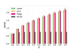
Figure 1: RMSE of $\mathbf{y}^{{}^{\prime}}$ and $\mathbf{y}$ on redwine dataset. The defender knows $\lambda$, $\beta$, and $\mathbf{z}$.

In the second experiment we relaxed the assumption that the defender knows $\lambda$, $\beta$ and $\mathbf{z}$, and instead simulated the practical scenario that the defender obtains estimates for these (for example, from historical attack data), but the estimates have error. We denote by $\hat{\lambda}=0.5$ and $\hat{\beta}=0.8$ the defender’s estimates of the true $\lambda$ and $\beta$. Remember that $\beta$ is the probability of an instance being malicious and $\lambda$ is negatively proportional to the attacker’s strength. So the estimation characterizes a pessimistic defender that is expecting very strong attacks. We experimented two kinds of estimation about $\mathbf{z}$: 1) the defender overestimates $\mathbf{z}$: $\hat{\mathbf{z}}=t\mathbf{1}$, where $t$ is a random variable sampled from a uniform distribution over $[5\sigma_{r},10]$; and 2) the defender underestimates $\mathbf{z}$: $\hat{\mathbf{z}}=t\mathbf{1}$, where $t$ is sampled from $[0,5\sigma_{r}]$. Due to space limitations we only present the results for the latter; the former can be found in the Appendix. In Figure 9 the y-axis represents the actual values of $\lambda$, and the x-axis represents the actual values of $\beta$. The color bar on the right of each figure visualizes the average RMSE. Each cell is averaged over 50 runs. The result shows that even if there is a discrepancy between the defender’s estimation and the actual adversarial behavior, MLSG is consistently more robust than the other approaches.

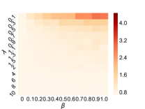
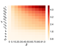
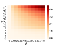
Figure 2: The average RMSE across different values of actual $\lambda$ and $\beta$ on redwine dataset. From left to right: MLSG, Lasso, Ridge, OLS.

The boston dataset: The response variables in boston dataset are the median prices of houses in Boston area. We define the attacker’s target as $\mathbf{z}=\mathbf{y}+\Delta$. The mean and standard deviation of $\mathbf{y}$ are $\mu_{b}=22.53$ and $\sigma_{b}=9.20$. We let $\Delta=2\sigma_{b}\times\mathbf{1}$. We first present the experimental result for best case in Figure 3. The result further supports our claim that proactively considering adversarial behavior can improve robustness.

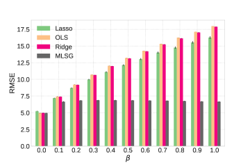
Figure 3: RMSE of $\mathbf{y}^{{}^{\prime}}$ and $\mathbf{y}$ on boston dataset. The defender knows $\lambda$, $\beta$, and $\mathbf{z}$.

We then relaxed the assumption that the defender knows $\lambda$, $\beta$ and $\mathbf{z}$ and set the defender’s estimates of the true $\lambda$ and $\beta$ as $\hat{\lambda}=0.1$ and $\hat{\beta}=0.3$. Similar to the experimental setting used on redwine dataset we experimented with overestimation and underestimation of $\mathbf{z}$. We show the results for overestimation in Figure 4, where $\hat{\mathbf{z}}=t\mathbf{1}$ and $t$ is sampled from $[2\sigma_{b},3\sigma_{b}]$. From Figure 4 we have several interesting observations. First, MLSG is more robust or equivalently robust compared with the three baselines, except when $\beta=0$. This is to be expected, as $\beta=0$ corresponds to non-adversarial data. Second, we observe that for large $\beta$, Lasso (middle left) and Ridge (middle right) are less robust than OLS (non-regularized linear regression) (rightmost). This is surprising, as Yang & Xu (2013) showed that Lasso-like algorithms (including Lasso and Ridge) are robust in the sense that their original optimization problems can be converted to min-max optimization problems, where the inner maximization takes malicious uncertainty about data into account. However, such robustness is only guaranteed if the regularization constant reflects the uncertainty interval; what our results suggest is when the interval bounds violated (i.e., regularization parameter is smaller than necessary), regularized models can actually degrade quickly.

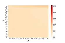
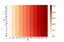
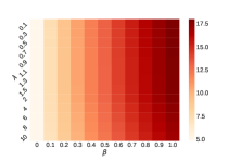
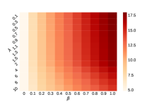
Figure 4: The average RMSE across different values of actual $\lambda$ and $\beta$ on boston dataset. From left to right: MLSG, Lasso, Ridge, OLS.

The PDF dataset: The response variables of this dataset are malicious scores ranging between 0 and 10. The mean and standard deviation of $\mathbf{y}$ are $\mu_{p}=5.56$ and $\sigma_{p}=2.66$. Instead of letting the $\Delta$ be non-negative as in previous two datasets, the attacker’s target is to descrease the scores of malicious PDFs. Consequently, we define $\Delta=-2\sigma_{p}\times\mathbf{1}_{\mathcal{M}}$, where $\mathcal{M}$ is the set of indices of malicious PDF and $\mathbf{1}_{\mathcal{M}}$ is a vector with only those elements indexed by $\mathcal{M}$ being one and others being zero. Our experiments were conducted on a subset (3000 malicious PDF and 3000 benign PDF) randomly sampled from the original dataset. We evenly divided the subset into training and testing sets. We applied PCA to reduce dimensionality of the data and selected the top-10 principal components as features. The result for best case is displayed in Figure 5. Notice that when $\beta=0$, MLSG is less robust than Lasso, as we would expect.

Similarly as before we relaxed the assumption that the defender knows $\lambda$, $\beta$ and $\mathbf{z}$ and let the defender’s estimation of the true $\lambda$ and $\beta$ be $\hat{\lambda}=1.5$ and $\hat{\beta}=0.5$. We also experimented with both overestimation and underestimation of $\mathbf{z}$. The defender’s estimation is $\hat{\mathbf{z}}=-t\mathbf{1}_{\mathcal{M}}$. For overestimation setting $t$ is sampled from $[2\sigma_{p},3\sigma_{p}]$, and for underestimation setting it is sampled from $[\sigma_{p},2\sigma_{p}]$. The result for underestimated $\hat{\mathbf{z}}$ is showed in Figure 6. Notice that in the leftmost plot of Figure 6 the area inside the blue rectangle corresponds to those cases where $\hat{\lambda}$ and $\hat{\beta}$ are overestimated and they are more robust than the remaining underestimated cases. Similar patterns can be observed in Figure 9. This further supports our claim that it is advantageous to overestimate adversarial behavior.

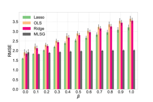
Figure 5: RMSE of $\mathbf{y}^{{}^{\prime}}$ and $\mathbf{y}$ on PDF dataset. The defender knows $\lambda$, $\beta$, and $\mathbf{z}$.

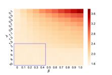
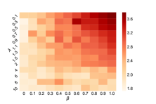
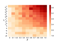
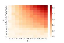
Figure 6: The average RMSE across different values of actual $\lambda$ and $\beta$ on PDF dataset. From left to right: MLSG, Lasso, Ridge, OLS.

7 Conclusion

We study the problem of linear regression in adversarial settings involving multiple learners learning from the same or similar data. In our model, learners first simultaneously decide on their models (i.e., learn), and an attacker then modifies test instances to cause predictions to err towards the attacker’s target. We first derive an upper bound on the cost functions of all learners, and the resulting approximate game. We then show that this game has a unique symmetric equilibrium, and present an approach for computing this equilibrium by solving a convex optimization problem. Finally, we show that the equilibrium is robust, both theoretically, and through an extensive experimental evaluation.

Appendix

7.1 Supplementary results for the redwine dataset

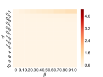
Figure 7: Overestimated $\mathbf{z}$, $\hat{\lambda}=0.5$, $\hat{\beta}=0.8$.The average RMSE across different values of actual $\lambda$ and $\beta$ on redwine dataset. From left to right: MLSG, Lasso, Ridge, OLS.

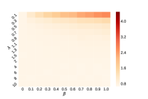
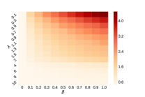
Figure 8: Overestimated $\mathbf{z}$, $\hat{\lambda}=1.5$, $\hat{\beta}=0.8$. The average RMSE across different values of actual $\lambda$ and $\beta$ on redwine dataset. From left to right: MLSG, Lasso, Ridge, OLS.

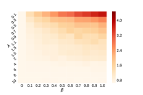
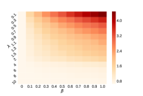
Figure 9: Underestimated $\mathbf{z}$, $\hat{\lambda}=1.5$, $\hat{\beta}=0.8$. The average RMSE across different values of actual $\lambda$ and $\beta$ on redwine dataset. From left to right: MLSG, Lasso, Ridge, OLS.

7.2 Supplementary results for the boston dataset

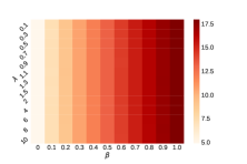
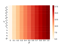
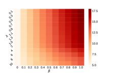
Figure 10: Underestimated $\mathbf{z}$, $\hat{\lambda}=0.3$, $\hat{\beta}=0.8$. The average RMSE across different values of actual $\lambda$ and $\beta$ on boston dataset. From left to right: MLSG, Lasso, Ridge, OLS.

7.3 Supplementary results for the PDF dataset

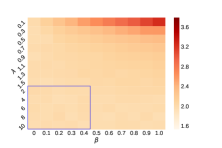
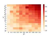
Figure 11: Overestimated $\mathbf{z}$, $\hat{\lambda}=1.5$, $\hat{\beta}=0.5$. The average RMSE across different values of actual $\lambda$ and $\beta$ on PDF dataset. From left to right: MLSG, Lasso, Ridge, OLS.

References

• Alfeld et al. (2016) Alfeld, S., Zhu, X., and Barford, P. Data poisoning attacks against autoregressive models. In AAAI Conference on Artificial Intelligence, 2016.
• Brückner & Scheffer (2011) Brückner, M. and Scheffer, T. Stackelberg games for adversarial prediction problems. In ACM SIGKDD international conference on Knowledge discovery and data mining, pp.  547–555, 2011.
• Cheng et al. (2004) Cheng, S.-F., Reeves, D. M., Vorobeychik, Y., and Wellman, M. P. Notes on equilibria in symmetric games. In International Workshop On Game Theoretic And Decision Theoretic Agents, pp.  71–78, 2004.
• Cortez et al. (2009) Cortez, P., Cerdeira, A., Almeida, F., Matos, T., and Reis, J. Modeling wine preferences by data mining from physicochemical properties. Decision Support Systems, 47(4):547–553, 2009.
• Dalvi et al. (2004) Dalvi, N., Domingos, P., Mausam, Sanghai, S., and Verma, D. Adversarial classification. In SIGKDD International Conference on Knowledge Discovery and Data Mining, pp.  99–108, 2004.
• Grosshans et al. (2013) Grosshans, M., Sawade, C., Brückner, M., and Scheffer, T. Bayesian games for adversarial regression problems. In International Conference on International Conference on Machine Learning, pp.  55–63, 2013.
• Harrison Jr & Rubinfeld (1978) Harrison Jr, D. and Rubinfeld, D. L. Hedonic housing prices and the demand for clean air. Journal of environmental economics and management, 5(1):81–102, 1978.
• Higham (1990) Higham, N. J. Analysis of the cholesky decomposition of a semi-definite matrix. In Reliable Numerical Computation, pp.  161–185. University Press, 1990.
• Laszka et al. (2016) Laszka, A., Lou, J., and Vorobeychik, Y. Multi-defender strategic filtering against spear-phishing attacks. In AAAI Conference on Artificial Intelligence, 2016.
• Li & Vorobeychik (2014) Li, B. and Vorobeychik, Y. Feature cross-substitution in adversarial classification. In Advances in neural information processing systems, pp. 2087–2095, 2014.
• Li & Vorobeychik (2015) Li, B. and Vorobeychik, Y. Scalable optimization of randomized operational decisions in adversarial classification settings. In Conference on Artificial Intelligence and Statistics, 2015.
• Lowd & Meek (2005) Lowd, D. and Meek, C. Adversarial learning. In Proceedings of the eleventh ACM SIGKDD international conference on Knowledge discovery in data mining, pp.  641–647. ACM, 2005.
• Rosen (1965) Rosen, J. B. Existence and uniqueness of equilibrium points for concave n-person games. Econometrica: Journal of the Econometric Society, pp. 520–534, 1965.
• Russu et al. (2016) Russu, P., Demontis, A., Biggio, B., Fumera, G., and Roli, F. Secure kernel machines against evasion attacks. In ACM Workshop on Artificial Intelligence and Security, pp.  59–69, 2016.
• Smith et al. (2017) Smith, A., Lou, J., and Vorobeychik, Y. Multidefender security games. IEEE Intelligent Systems, 32(1):50–60, 2017.
• Šrndic & Laskov (2014) Šrndic, N. and Laskov, P. Practical evasion of a learning-based classifier: A case study. In 2014 IEEE Symposium on Security and Privacy, pp. 197–211, 2014.
• Stevens & Lowd (2013) Stevens, D. and Lowd, D. On the hardness of evading combinations of linear classifiers. In ACM Workshop on Artificial Intelligence and Security, 2013.
• Vorobeychik et al. (2011) Vorobeychik, Y., Mayo, J. R., Armstrong, R. C., and Ruthruff, J. Noncooperatively optimized tolerance: Decentralized strategic optimization in complex systems. Physical Review Letters, 107(10):108702, 2011.
• Xu et al. (2009) Xu, H., Caramanis, C., and Mannor, S. Robust regression and lasso. In Advances in Neural Information Processing Systems, pp. 1801–1808, 2009.
• Yang & Xu (2013) Yang, W. and Xu, H. A unified robust regression model for lasso-like algorithms. In International Conference on Machine Learning, pp. 585–593, 2013.
• Zhou et al. (2012) Zhou, Y., Kantarcioglu, M., Thuraisingham, B. M., and Xi, B. Adversarial support vector machine learning. In ACM SIGKDD International Conference on Knowledge Discovery and Data Mining, pp.  1059–1067, 2012.