Area law and universality in the statistics of subsystem energy

Abstract

We introduce Rényi entropy of a subsystem energy as a natural quantity which closely mimics the behavior of the entanglement entropy and can be defined for all quantum many body systems. In other words, consider a quantum chain in its ground state and then, take a subdomain of this system with natural truncated Hamiltonian. Since the total Hamiltonian does not commute with the truncated Hamiltonian, the subsystem can be in one of its eigenenergies with different probabilities. Using the fact that the global energy eigenstates are locally close to diagonal in the local energy eigenbasis, we argue that the Rényi entropy of these probabilities follows an area law for the gapped systems. When the system is at the critical point, the Rényi entropy follows a logarithmic behavior with a universal coefficient. Consequently, our quantity not only detects the phase transition but also determines the universality class of the critical point. Moreover we show that the largest defined probabilities are very close to the biggest Schmidt coefficients. We quantify this by defining a truncated Shannon entropy which its value is almost indistinguishable from the truncated von Neumann entanglement entropy. Compare to the entanglement entropy, our quantity has the advantage of being associated to a natural observable (subsystem Hamiltonian) that can be defined (and probably measured) easily for all the short-range interacting systems. We support our arguments by detailed numerical calculations performed on the transverse field XY-chain.

I Introduction

Quantum information theory and particularly the concept of entanglement has played an increasingly important role in condensed matter and high energy physics in recent years. More specifically, it has been very useful in the study of different phases of many body quantum systems Amico2008 ; Affleck2009 ; Moore2009 ; Peschel2009 ; Cramers2010 ; Modi2012 ; Laflorencie2016 ; Chiara2017 , structure of quantum field theories CC2009 ; Doyon2009 ; Casini2009 and understanding the gravityTakayanagibook ; Nishioka2018 . Most of these studies are directly related to the concept of entropy which can be defined when there is a probability distribution. The Shannon entropy and its natural generalizations, the Rényi entropies, are the building blocks of the classical information theory. They can be also used as the starting point to define and understand the quantum version of the entropy. The Rényi entropy for $\alpha\geq 0$ is defined as

$$H_{\alpha}=\frac{1}{1-\alpha}\ln\sum_{i=1}^{n}p_{i}^{\alpha},$$ (1)

where $p_{i}$’s are the corresponding probabilities. For $\alpha=1$, one can recover the Shannon entropy $H_{1}=-\sum_{i=1}^{n}p_{i}\ln p_{i}$. To see how the above quantities can be used to study the quantum many-body systems and especially quantum phase transitions, consider a quantum system in its ground state $|\psi_{g}\rangle$. Since in quantum mechanics we have normally infinite number of observables we have the freedom to write the ground state in the basis of one of them as $|\psi_{g}\rangle=\sum_{I}a_{I}|I\rangle$, where $|I\rangle$ is one of the eigenstates of the considered observable and $p_{I}=|a_{I}|^{2}$ is the probability of finding the corresponding eigenvalue. These probabilities can be used to define the Shannon entropy and one of the immediate consequences is the entropic uncertainty relation uncertainty . By choosing an appropriate local observable, for example, spin, one can use the Shannon entropy to detect the phase transitions and restricted versions of universalities estephan2010a ; estaphan2010b ; Fradkin2007 ; Oshikawa2017 . The situation is even more interesting when one considers the marginal probabilities in a subsystem. When the corresponding observable is a local quantity, the associated probabilities are called formation probabilities and it is known that especial type of them can be used to determine the central charge and the universality class of the critical points Estephan2014 ; Rajabpour2015 ; Najafi2016 ; Rajabpour2016 . For local observables, it is natural to expect that the Shannon(Rényi) entropy be proportional with the size of the subsystem (volume-law)footnotevolumelaw which makes the leading term non-universal and less interesting. However, numerous numerical calculations suggest that for critical quantum chains, the subleading term follows a logarithmic behavior with respect to the subsystem size with a coefficient which is universal and connected to the central charge AR2013 ; estephan2014b ; AR2014 ; AR2015 ; Najafi2016 ; Alcaraz2016 . For other related studies see Refs.Luitz2014a ; Luitz2014b ; Luitz2015c . Although from the experimental point of view, the Shannon (Rényi) entropy of local observables in a subsystem looks a natural quantity, theoretically, it is interesting to make the quantity ”basis independent” by minimizing over all the possible bases. This minimization leads to the von Neumann entanglement entropy and its generalizations quantum Rényi entropiesWildeBook . For a density matrix $\rho$, the quantum Rényi entropy for $\alpha\geq 0$ is

$$S_{\alpha}=\frac{1}{1-\alpha}\ln\text{tr}\rho^{\alpha}.$$ (2)

For $\alpha=1$, we recover the von Neumann entropy $S=-\text{tr}\rho\ln\rho$. If we consider the total system be in a pure state (for example, the ground state) and calculate the reduced density matrix for a subsystem and plug this matrix in the above equation, we end up with the entanglement entropy of the subsystem with respect to its complement. Another way of looking to this quantity is by calculating the Shannon entropy in the Schmidt basis, which is a complicated non-local basis that minimizes the entropy. von Neumann entropy has been studied in a myriad of articles, for review see Refs. Amico2008 ; CC2009 ; Doyon2009 ; Affleck2009 ; Moore2009 ; Peschel2009 ; Casini2009 ; Cramers2010 ; Modi2012 ; Laflorencie2016 ; Takayanagibook ; Chiara2017 ; Nishioka2018 . The most relevant results for our purpose are the followings: the entanglement entropy of the ground state for gapped systems follows an area law Hastings2008 ; Cramers2010 ; Brandao2013 ; Vazirani2012 ; Brandao2015 . For infinitely long one dimensional critical systems the Rényi (von Neumann) entropy of a subsystem with size $l$ is given byHolzhy1994 ; Vidal2003 ; CC2004

$$S_{\alpha}=\frac{c}{6}(1+\frac{1}{\alpha})\ln l+\gamma_{\alpha},$$ (3)

where $c$ is the central charge of the underlying conformal field theory and $\gamma_{\alpha}$ is a non-universal constant. Based on the above results, one can make the following argument: Shannon entropy of a subsystem for local observables (basis) follows a volume law but it follows an area law (logarithmic law) in gapped (critical) systems for non-local Schmidt basis. This makes one to believe that there should be some non-local observables in between these two extreme cases. For example, one can think about the total number of particles in a subsystem and study its distribution as it has been done in the context of full counting statistics Eisler2003 ; Klich2006 ; Klich2009 ; Calabrese2012 ; Rachel2012a ; Rachel2012b ; Klich2014 ; FCS . One can also study other quantities such as the total magnetization distribution Fendley2008 or the distribution of the subsystem energy Najafi2017 .

Among the many natural non-local quantities that one can study, we are interested in the one which, apart from being natural, can be defined for all the quantum chains and can mimic in the best way the entanglement entropy of a subsystem. Since the von Neumann entropy is defined without reference to the observable of the system, it is widely believed that the direct measurement of this quantity is impossible due to the fact that this quantity is nonlocal and it’s measurement requires knowledge about the full reduced density matrix which grows exponentially with the size of the system. An observable such as the truncated Hamiltonian that its statistics closely mimics the entanglement Hamiltonian is not only interesting by itself, might also be useful in a better theoretical and experimental understanding of the entanglement entropy.

In this paper, we argue that the subsystem energy is such a quantity. Its Rényi entropy follows an area law for the gapped systems and it is logarithmic for the critical systems. The coefficient of the logarithm is universal and may well be related to the central charge. Compare to the entanglement entropy the Shannon(Rényi) entropy of a subsystem energy has the advantage that it is related to a natural observable which not only can be defined easily but also measured simply for the short-range interacting systems. The paper is organized as follows: in sec. II, based on some known results we first argue that the statistics of the subsystem energy is a perfect candidate which can mimic the entanglement entropy. Then, in sec III, we develop an elegant method to calculate the distribution of the eigenvalues of the quadratic observables in the free fermionic systems and provide an exact formula for the probabilities in the basis of the subsystem energy. Then, in section IV, we study the Rényi entropy of the subsystem energy for the transverse field XY chain numerically to demonstrate the validity of the arguments. We further provide our results to confirm the Rényi entropy of subsystem energy with the Rényi entanglement entropy. Finally, in section V, we comment on the possible experimental setups that can be used to measure the subsystem energy Shannon entropy.

II subsystem energy basis

We start by considering a generic nearest neighbor Hamiltonian of an infinite systemfootnote1 $\textbf{H}=\sum_{i=-\infty}^{\infty}H_{i,i+1}$, where $H_{i,i+1}$ has support in the set of sites $i$ and $i+1$. Now, consider $l$ contiguous sites and define a truncated Hamiltonian for the subsystem as $\textbf{H}_{l}=\sum_{i=1}^{l-1}H_{i,i+1}$. For interacting Hamiltonians, we always have $[\textbf{H},\textbf{H}_{l}]\neq 0$, which means that if the total system is in its ground state, the subsystem can be in different eigenstates $|e_{j}\rangle$ with different probabilities $p(e_{j})$. Note that for the short-range Hamiltonians the right-hand side of $[\textbf{H},\textbf{H}_{l}]$ is dependent just on the boundary terms which hints on ”weak” uncertainty relations. To study the corresponding probabilities, one can first calculate the reduced density matrix of the subsystem $\rho_{l}=\text{tr}_{\bar{l}}|\psi_{g}\rangle\langle\psi_{g}|$ where the trace is over the complement of the subsystem. The reduced density matrix is exactly diagonal in the Schmidt basis which leads to the quantum entanglement entropy, but it has off-diagonal terms in every other basis. However, an interesting theorem is proved in Ref. muller2015 , see also Ref.Arad2016 ; which indicates that global energy eigenstates are locally close to diagonal in the local energy eigenbasisfootnote2 . In other words, the reduced density matrix is weekly diagonalfootnote2 in the eigenbasis of the truncated Hamiltonian. This theorem suggests that the eigenbasis of the subsystem Hamiltonian is not that much different from the Schmidt basis. It is equivalent to say that $p(e_{j})$’s are close to the Schmidt coefficients. One can then guess that although the Rényi entropy calculated by using $p(e_{j})$’s is for sure bigger than the Rényi entanglement entropy, it should not be too far from it. For example, one can guess that the Rényi entropy in this case follows the area law for gapped systems and has logarithmic behavior for critical systems. In the rest of this paper, we will show that indeed this argument is correct and the Rényi entropy of the subsystem energy follows closely the Rényi entanglement entropy.

III Subsystem energy probabilities in the XY chain

The Hamiltonian of the XY-chain is defined as

$$\textbf{H}_{XY}=\hskip 213.39566pt$$

$$-J\sum_{j=1}^{L}\Big{[}(\frac{1+\gamma}{4})\sigma_{j}^{x}\sigma_{j+1}^{x}+(\frac{1-\gamma}{4})\sigma_{j}^{y}\sigma_{j+1}^{y}\Big{]}-\frac{h}{2}\sum_{j=1}^{L}\sigma_{j}^{z},\hskip 17.07182pt$$ (4)

where the $\sigma_{j}^{\alpha}$ ($\alpha=x,y,z$) are Pauli matrices. $J>0$ is the spin coupling, $\gamma$ is the anisotropic parameter and, $h$ is the external magnetic field. For $\gamma=1$, and $\gamma=0$, the XY model reduces to the Ising spin chain and XX chain, respectively. The phase diagram of the model is rich, there are two different critical lines with different universality classes corresponding to the central charges of $c=1$ and $c=\frac{1}{2}$ for the critical XX line $0\leq h<1$ and the critical XY line $h=1$, respectively.

To calculate the statistics of the subsystem energy we first need to write the above Hamiltonian in a more suitable form. Introducing canonical spinless fermions through the Jordan-Wigner transformation, $c_{l}^{\dagger}=\prod_{n<l}\sigma_{n}^{z}\sigma_{l}^{+}$, the Hamiltonian (III) becomes

$$\ \textbf{H}=\textbf{c}^{\dagger}.\hat{\textbf{A}}.\textbf{c}+\frac{1}{2}\textbf{c}^{\dagger}.\hat{\textbf{B}}.\textbf{c}^{\dagger}+\frac{1}{2}\textbf{c}.\hat{\textbf{B}}^{T}.\textbf{c}-\frac{1}{2}{\rm Tr}{\hat{\textbf{A}}},$$ (5)

with appropriate $\hat{\textbf{A}}$ and $\hat{\textbf{B}}$ matrices. We use the hat symbol to indicate the matrices for the total system, while the symbols without hat will indicate the subsystem. The method that we present here is quite general and can be used for any Hamiltonian with $\hat{\textbf{A}}$ and $\hat{\textbf{B}}$ being symmetric and anti-symmetric matricesfootnote3 . For the truncated Hamiltonian $\textbf{H}_{D}$ (for quantum chains $D=l$), the same form of the Hamiltonian can be used. Although the method can be generalized for more general states, we consider that the total system is in its ground state. To this end, the probability of the subsystem in different energy states can be calculated from the reduced density matrix by using the standard method of Refs. Peschel ; Barthel2006 ; Peschel2009 . The starting point is the following reduced density matrix Barthel2006 written in fermionic coherent basis:

$$\rho_{D}(\boldsymbol{\xi},\boldsymbol{\xi^{\prime}}) = <\boldsymbol{\xi}|\rho_{D}|\boldsymbol{\xi^{\prime}}>$$ (6)

$$= \det\frac{1}{2}(\mathbb{I}-\textbf{G})e^{\frac{1}{2}(\bar{\boldsymbol{\xi}}-\boldsymbol{\xi}^{\prime})^{T}\textbf{F}(\bar{\boldsymbol{\xi}}+\boldsymbol{\xi}^{\prime})},$$

where we have $\textbf{F}=(\textbf{G}+\mathbb{I})(\mathbb{I}-\textbf{G})^{-1}$ with G being the correlation matrix with the elements $G_{ij}=\langle(c_{i}^{\dagger}-c_{i})(c_{j}^{\dagger}+c_{j})\rangle$. In the above, we introduced the fermionic coherent state as follows,

$$|\boldsymbol{\xi}\rangle=|\xi_{1},\xi_{2},...,\xi_{|D|}\rangle=e^{-\sum_{k=1}^{|D|}\xi_{{}_{k}}c_{k}^{\dagger}}|0\rangle,$$ (7)

where $\xi_{k}$’s are Grassmann numbers which satisfy the following properties: $\xi_{n}\xi_{m}+\xi_{m}\xi_{n}=0$ and $\xi_{n}^{2}=\xi_{m}^{2}=0$. Then, it is straightforward to show that

$$c_{k}|\boldsymbol{\xi}>=\xi_{k}|\boldsymbol{\xi}>.$$ (8)

If we expand the exponential (6), we can rewrite it as,

$$\rho_{D}(\boldsymbol{\xi},\boldsymbol{\xi^{\prime}})=\det\frac{1}{2}(\mathbb{I}-\textbf{G})e^{\frac{1}{2}\bar{\boldsymbol{\xi}}\textbf{F}\bar{\boldsymbol{\xi}}}\,\,e^{\frac{1}{2}\bar{\boldsymbol{\xi}}(\textbf{F}+\textbf{F}^{T})\boldsymbol{\xi}^{\prime}}\,\,e^{-\frac{1}{2}\boldsymbol{\xi}^{\prime}\textbf{F}\boldsymbol{\xi}^{\prime}},\hskip 28.45274pt$$ (9)

We notice that, $\frac{\bar{\boldsymbol{\xi}}\textbf{F}\bar{\boldsymbol{\xi}}-\bar{\boldsymbol{\xi}}\textbf{F}^{T}\bar{\boldsymbol{\xi}}}{2}=\bar{\boldsymbol{\xi}}\textbf{F}\bar{\boldsymbol{\xi}}$. Then, we get,

$$\rho_{D}(\boldsymbol{\xi},\boldsymbol{\xi^{\prime}})=\det\frac{1}{2}(\mathbb{I}-\textbf{G})e^{\frac{1}{2}\bar{\boldsymbol{\xi}}\textbf{F}_{a}\bar{\boldsymbol{\xi}}}\,\,e^{\frac{1}{2}\bar{\boldsymbol{\xi}}\textbf{F}_{s}\boldsymbol{\xi}^{\prime}}\,\,e^{-\frac{1}{2}\boldsymbol{\xi}^{\prime}\textbf{F}_{a}\boldsymbol{\xi}^{\prime}},\hskip 28.45274pt$$ (10)

where $\textbf{F}_{a}=\frac{\textbf{F}-\textbf{F}^{T}}{2}$ and $\textbf{F}_{s}=\frac{\textbf{F}+\textbf{F}^{T}}{2}$. By converting the Grassmann variables to fermionic operators, we have,

$$\rho_{D}=\det\frac{1}{2}(\mathbb{I}-\textbf{G})e^{\frac{1}{2}\textbf{c}^{\dagger}\textbf{F}_{a}\textbf{c}^{\dagger}}\,\,e^{\frac{1}{2}\textbf{c}^{\dagger}\ln(\textbf{F}_{s})\textbf{c}}\,\,e^{-\frac{1}{2}\textbf{c}\textbf{F}_{a}\textbf{c}},$$ (11)

We would like to write the reduced density matrix as

$$\rho_{D}=\det\frac{1}{2}(\mathbb{I}-\textbf{G})e^{\mathcal{H}}$$ (12)

Where $\mathcal{H}$ is the entanglement Hamiltonian that can be calculated by combining the exponential terms in the equation  11. In other words, we would like to have

$$\ \mathcal{H}=\sum_{lm}[c_{l}^{\dagger}M_{lm}c_{m}+\frac{1}{2}c_{l}^{\dagger}N_{lm}c_{m}^{\dagger}+\frac{1}{2}c_{l}N_{ml}c_{m}]-\frac{1}{2}{\rm Tr}{\textbf{M}},$$ (13)

where M and N are symmetric and antisymmetric matrices. They can be calculated using Balian-Brezin formula Balian1969

$$\ \textbf{T}=e^{\begin{pmatrix}\textbf{M}&\textbf{N}\\ \textbf{-N}&\textbf{-M}\\ \end{pmatrix}}=\begin{pmatrix}\textbf{T}_{11}&\textbf{T}_{12}\\ \textbf{T}_{21}&\textbf{T}_{22}\\ \end{pmatrix}=\begin{pmatrix}\textbf{F}_{s}-\textbf{F}_{a}\textbf{F}_{s}^{-1}\textbf{F}_{a}&\textbf{F}_{a}\textbf{F}_{s}^{-1}\\ -\textbf{F}_{s}^{-1}\textbf{F}_{a}&\textbf{F}_{s}^{-1}\\ \end{pmatrix}.$$ (14)

Then, we get

$$\ \begin{pmatrix}\textbf{M}&\textbf{N}\\ \textbf{-N}&\textbf{-M}\\ \end{pmatrix}=\ln\begin{pmatrix}\textbf{F}_{s}-\textbf{F}_{a}\textbf{F}_{s}^{-1}\textbf{F}_{a}&\textbf{F}_{a}\textbf{F}_{s}^{-1}\\ -\textbf{F}_{s}^{-1}\textbf{F}_{a}&\textbf{F}_{s}^{-1}\\ \end{pmatrix}.$$ (15)

Now, we can rewrite the entanglement Hamiltonian as follows

$$\ \mathcal{H}=\frac{1}{2}(\textbf{c}^{\dagger}\,\,\textbf{c})\begin{pmatrix}\textbf{M}&\textbf{N}\\ -\textbf{N}&-\textbf{M}\\ \end{pmatrix}\begin{pmatrix}\textbf{c}\\ \textbf{c}^{\dagger}\\ \end{pmatrix}+\frac{1}{2}{\rm Tr}\ln{(\textbf{F}_{s})}.$$ (16)

The second step is to diagonalize the truncated Hamiltonian $\textbf{H}_{D}$ with the standard method of Ref.LSM , see Appendix A. The idea is based on canonical transformation

$$\ \begin{pmatrix}\textbf{c}\\ \textbf{c}^{\dagger}\\ \end{pmatrix}=\textbf{U}^{\dagger}\begin{pmatrix}\boldsymbol{\eta}\\ \boldsymbol{\eta}^{\dagger}\\ \end{pmatrix}.$$ (17)

By using the above relation , we can rewrite the entanglement Hamiltonian with respect to the $\eta_{k}$’s as follows:

$$\ \mathcal{H} = \frac{1}{2}(\boldsymbol{\eta}^{\dagger}\,\,\boldsymbol{\eta})\textbf{U}\begin{pmatrix}\textbf{M}&\textbf{N}\\ -\textbf{N}&-\textbf{M}\\ \end{pmatrix}\textbf{U}^{\dagger}\begin{pmatrix}\boldsymbol{\eta}\\ \boldsymbol{\eta}^{\dagger}\\ \end{pmatrix}+\frac{1}{2}{\rm Tr}\ln{(\textbf{F}_{s})}$$ (18)

$$= \frac{1}{2}(\boldsymbol{\eta}^{\dagger}\,\,\boldsymbol{\eta})\textbf{Q}\begin{pmatrix}\boldsymbol{\eta}\\ \boldsymbol{\eta}^{\dagger}\\ \end{pmatrix}+\frac{1}{2}{\rm Tr}\ln{(\textbf{F}_{s})},$$

where

$$\ \textbf{Q}=\begin{pmatrix}\textbf{Q}_{11}&\textbf{Q}_{12}\\ \textbf{Q}_{21}&\textbf{Q}_{22}\\ \end{pmatrix}=\textbf{U}\begin{pmatrix}\textbf{M}&\textbf{N}\\ -\textbf{N}&-\textbf{M}\\ \end{pmatrix}\textbf{U}^{\dagger}.$$ (19)

The reduced density matrix in the $\eta$ basis finally becomes:

$$\rho_{D}=\det\frac{1}{2}(\mathbb{I}-\textbf{G})[{\rm\det}(\textbf{F}_{s})]^{\frac{1}{2}}e^{\frac{1}{2}(\boldsymbol{\eta}\,\,\boldsymbol{\eta}^{\dagger})\begin{pmatrix}\textbf{Q}_{11}&\textbf{Q}_{12}\\ \textbf{Q}_{21}&\textbf{Q}_{22}\\ \end{pmatrix}\begin{pmatrix}\boldsymbol{\eta}\\ \boldsymbol{\eta}^{\dagger}\\ \end{pmatrix}}.\hskip 14.22636pt$$ (20)

Now, we define the coherent basis of the $\eta$ representation as

$$\eta_{k}|\boldsymbol{\gamma}>=\gamma_{k}|\boldsymbol{\gamma}>.$$ (21)

Using the above basis, we have

$$\langle\boldsymbol{\gamma}|\rho_{D}|\boldsymbol{\gamma}^{\prime}\rangle=\det\frac{1}{2}(\mathbb{I}-\textbf{G})[{\rm\det}(\textbf{F}_{s})]^{\frac{1}{2}}\langle\boldsymbol{\gamma}|e^{\frac{1}{2}(\boldsymbol{\eta}^{\dagger}\,\,\boldsymbol{\eta})\begin{pmatrix}\textbf{Q}_{11}&\textbf{Q}_{12}\\ \textbf{Q}_{21}&\textbf{Q}_{22}\\ \end{pmatrix}\begin{pmatrix}\boldsymbol{\eta}\\ \boldsymbol{\eta}^{\dagger}\\ \end{pmatrix}}|\boldsymbol{\gamma}^{\prime}\rangle.$$ (22)

To calculate the above equation we first define $\tilde{\textbf{T}}$ matrix,

$$\tilde{\textbf{T}}=e^{\textbf{Q}}=\textbf{U}\begin{pmatrix}\textbf{F}_{s}-\textbf{F}_{a}\textbf{F}_{s}^{-1}\textbf{F}_{a}&\textbf{F}_{a}\textbf{F}_{s}^{-1}\\ -\textbf{F}_{s}^{-1}\textbf{F}_{a}&\textbf{F}_{s}^{-1}\\ \end{pmatrix}\textbf{U}^{\dagger}.$$ (23)

and

$$\ \tilde{\textbf{X}} = \tilde{\textbf{T}}_{12}(\tilde{\textbf{T}}_{22})^{-1},$$

$$\tilde{\textbf{Z}} = (\tilde{\textbf{T}}_{22}^{-1})\tilde{\textbf{T}}_{21},$$

$$e^{-\tilde{\textbf{Y}}} = \tilde{\textbf{T}}_{22}^{T}.$$ (24)

Then, by decomposing the exponential factor in the equation 22 (using the Balian-Brezin formula Balian1969 ), we get

$$\langle\boldsymbol{\gamma}|\rho_{D}|\boldsymbol{\gamma}^{\prime}\rangle=\det\frac{1}{2}(\mathbb{I}-\textbf{G})[{\rm\det}(\textbf{F}_{s})]^{\frac{1}{2}}\hskip 56.9055pt$$

$$\times\langle\boldsymbol{\gamma}|e^{\frac{1}{2}\boldsymbol{\eta}^{\dagger}\tilde{\textbf{X}}\boldsymbol{\eta}^{\dagger}}\,\,e^{\boldsymbol{\eta}^{\dagger}\tilde{\textbf{Y}}\boldsymbol{\eta}}\,\,e^{\frac{1}{2}\boldsymbol{\eta}\tilde{\textbf{Z}}\boldsymbol{\eta}}\,\,e^{-\frac{1}{2}{\rm Tr}{\tilde{\textbf{Y}}}}|\boldsymbol{\gamma}^{\prime}\rangle,$$ (25)

which becomes,

$$\langle\boldsymbol{\gamma}|\rho_{D}|\boldsymbol{\gamma}^{\prime}\rangle=\det\frac{1}{2}(\mathbb{I}-\textbf{G})\hskip 113.81102pt$$

$$\times[{\rm\det}(\textbf{F}_{s})]^{\frac{1}{2}}\,\,e^{\frac{1}{2}\bar{\boldsymbol{\gamma}}\tilde{\textbf{X}}\bar{\boldsymbol{\gamma}}}\,\,e^{\bar{\boldsymbol{\gamma}}e^{\tilde{\textbf{Y}}}\boldsymbol{\gamma^{\prime}}}\,\,e^{\frac{1}{2}\boldsymbol{\gamma^{\prime}}\tilde{\textbf{Z}}\boldsymbol{\gamma^{\prime}}}\,\,e^{-\frac{1}{2}{\rm Tr}{\tilde{\textbf{Y}}}}.\hskip 28.45274pt$$ (26)

After defining

$$\tilde{\textbf{F}}_{s} = e^{\tilde{\textbf{Y}}},$$

$$\tilde{\textbf{F}} = \tilde{\textbf{F}}_{s}+\tilde{\textbf{F}}_{a}=\tilde{\textbf{X}}+e^{\tilde{\textbf{Y}}},$$ (27)

the reduced density matrix becomes,

$$\langle\boldsymbol{\gamma}|\rho_{D}|\boldsymbol{\gamma}^{\prime}\rangle=\det\frac{1}{2}(\mathbb{I}-\textbf{G})[{\rm\det}(\textbf{F}_{s})]^{\frac{1}{2}}e^{-\frac{1}{2}{\rm Tr}\tilde{\textbf{Y}}}\,\,e^{\frac{1}{2}(\bar{\boldsymbol{\gamma}}-\boldsymbol{\gamma^{\prime}})\tilde{\textbf{F}}(\bar{\boldsymbol{\gamma}}+\boldsymbol{\gamma^{\prime}})}=\det\frac{1}{2}(\mathbb{I}-\textbf{G})[\frac{{\rm\det}(\textbf{F}_{s})}{{\rm\det}(\tilde{\textbf{F}}_{s})}]^{\frac{1}{2}}\,\,e^{\frac{1}{2}(\bar{\boldsymbol{\gamma}}-\boldsymbol{\gamma^{\prime}})\tilde{\textbf{F}}(\bar{\boldsymbol{\gamma}}+\boldsymbol{\gamma^{\prime}})}.$$ (28)

At this point, we explain how one can use the above equation to calculate the desired probabilities. The procedure is similar to the calculation of formation probabilitiesNajafi2016 . First of all, one can think of $|\boldsymbol{\gamma}\rangle$ as a coherent state corresponding to the different excitation modes. For example, when all the $\gamma_{k}$’s are zero the corresponding coherent state is equal to the vacuum (no excited modes). In this case, it is easy to see that to find the probability of a subsystem in its ground state, one needs to put all the $\gamma$’s equal to zero, then

$$p(e_{g})=\det\frac{1}{2}(\mathbb{I}-\textbf{G})[\frac{{\rm\det}(\textbf{F}_{s})}{{\rm\det}(\tilde{\textbf{F}}_{s})}]^{\frac{1}{2}}.$$ (29)

To find the probability of other energies, one needs to know the corresponding modes $\lambda_{k}$’s in which generate the desired energy. This means in the corresponding coherent state we put one fermion in the $\eta$ basis which simply is equivalent to the following Grassmann integration

$$|0,0,...,1_{k},0,...,0\rangle=\int d\gamma_{k}|\boldsymbol{\gamma}\rangle.$$ (30)

The left hand side is the excited state with the mode $k$ excited. It should now be clear that if we want to calculate the probability of the corresponding state we just need to first put $\boldsymbol{\gamma}^{\prime}=\boldsymbol{\gamma}$ and then put all the modes that are not excited equal to zero and then Grassmann integrate over $\gamma_{k}$. This will lead to the one of the principal minors of the matrix $\tilde{\textbf{F}}$. The procedure is the same when we excite more modes that lead to the other excited states. There are $2^{|D|}$ possible mode excitations which correspond to the same number of principal minors that the matrix $\tilde{\textbf{F}}$ have. One should note that sometimes different mode excitations lead to the same energy for the excited state. In this cases, we need to sum the minors. One can now summarize the main equation of the article as

$$p(e)=\det\frac{1}{2}(\mathbb{I}-\textbf{G})[\frac{{\rm\det}(\textbf{F}_{s})}{{\rm\det}(\tilde{\textbf{F}}_{s})}]^{\frac{1}{2}}\sum_{e}\text{Min}[\tilde{\textbf{F}}],$$ (31)

where the sum is over the degeneracy of the energy $e$. In the end, in Appendix B, we drive an explicit formula for the generating function of the subsystem energy.

IV Rényi entropy of the subsystem energy

Using the equation (31), we first, calculated the Rényi entropy of the subsystem energy for different gapped points of an infinite XY chain and verified the area law for $\alpha\geq\alpha_{c}$, see Figure 1; where $\alpha_{c}$ seems to be close to onefootnotealphac . Then, we calculated the same quantity for the critical regions which shows the logarithmic behavior for the Rényi entropy, see Figure 1.

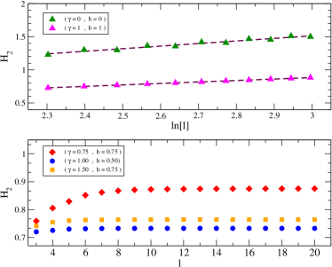
Figure 1: (color online)Up: logarithmic behavior of the Rényi entropy, $\alpha=2$, of the subsystem energy of the critical XY chain for $\gamma=h=0$ and $\gamma=h=1$. Down: Area law of the Rényi entropy for various values of the parameters of the gapped XY chain.

In general, for the Rényi entropy, we find

$$H_{\alpha}=\epsilon(\alpha)\ln l+\beta_{\alpha},$$ (32)

for $l\geq 6$. Afterwards, in the Figure 2, we verified that these coefficients are universal in the sense that on the critical XX and XY lines, their values do not change significantly. We note that there is a freedom in choosing the boundary conditions of the truncated Hamiltonian. To check that these numbers are insensitive to these boundary conditions, we also considered periodic boundary conditions for $H_{l}$ and repeated the calculations and reached to the same numbers. Note that in calculating the Shannon (Rényi) entropy, we use all the probabilities including those that are associated with very high energies in the subsystem. These states which are far from the ground state normally do not show universal behavior and one can not describe them by quantum field theories. Our calculations indicates that, in the scaling limit, most probably the contribution of these states in the calculation of the Shannon entropy is negligiblefootnotesmallP . In the Figure 3, we plotted the $\frac{\epsilon(\alpha)}{c}$ and the coefficient of the logarithm in the equation (3) for the XX and critical Ising chain. Remarkably, they follow a very similar behavior which confirms our original discussion regarding the closeness of the local energy basis to the Schmidt basis.

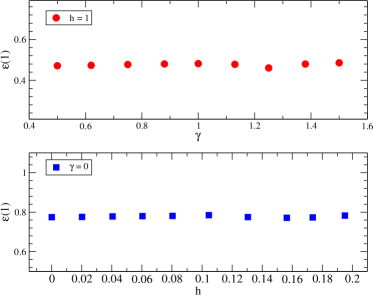
Figure 2: (color online) Universality of the coefficient of the logarithm, $\epsilon(1)$ on the critical XY line, i.e. $h=1$ and critical XX line, i.e. $\gamma=0$. Here, the fits are performed using the subsystem sizes $8\leq l\leq 16$.

It also indicates that probably (at least for large $\alpha$’s) the coefficient $\epsilon(\alpha)$ is linearly proportional to the central charge. For small $\alpha$’s the deviations between the three graphs are more significant which should not be surprising since here, the more important probabilities are the smaller ones which are related to the very high excited states of the subsystem Hamiltonian. We also noticed that in the regime $\alpha<0.5$ for the considered sizes $l\leq 20$ we do not see a nice logarithmic behavior.

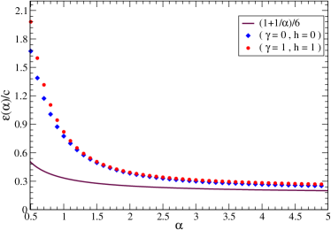
Figure 3: (color online)$\frac{\epsilon(\alpha)}{c}$ for the critical XX, i.e. $\gamma=h=0$ and the critical Ising, i.e. $\gamma=h=1$ with respect to $\alpha$. The solid line is the CFT result for the Rényi entanglement entropy. Here, the fits are performed using the subsystem sizes $8\leq l\leq 16$.

Since the number of possible energies for the subsystem increases exponentially with the subsystem size there is a limitation in calculating the Shannon entropy for large subsystems. That makes the estimation of the coefficient $\epsilon(\alpha)$ very difficult. Instead of the Shannon entropy if one considers $\alpha\to\infty$, then, the only probability that one needs to take into account is the probability of the subsystem being in the ground state which is the largest probability. In this case, one can go to relatively large sizes about $l=1000$ and check all the conclusions with much more accuracy. Indeed, we were able to calculate the coefficient of the logarithm in this case with high accuracy for the XX and critical Ising chain:

$$\epsilon_{XX}(\infty)=0.222(2),\hskip 28.45274pt\epsilon_{Ising}(\infty)=0.112(2).$$ (33)

We also checked the universality of these values on the critical line, see Appendix C. For the semi-infinite systems, the coefficients are within one percent from the half of the above values. Note that this quantity is different from the quantity called fidelity in Refs.Dubail2011 ; Dubail2013 . In the following we further support our ideas by first introducing the truncated Shannon and compare it with the entanglement entropy of the subsystem energy. Furthermore, we provide comprehensive numerical results on the closeness of Rényi entanglement entropy and Rényi entropy of the subsystem energy and Schmidt basis and the truncated Hamiltonian basis.

IV.1 Truncated Shannon and entanglement entropy of the subsystem energy

All of the results that we presented so far indicate the closeness of our probabilities $p_{j}$ to the Schmidt coefficients $\lambda_{j}$. Most interestingly similar to the Schmidt coefficients we realized that just the first few probabilities are big and the rest are very smallfootnotesmall . To show how much these probabilities are close to the Schmidt coefficients and see their contribution to the full Shannon entropy it is useful to define a truncated Shannon and truncated von Neumann entropy footnotetruncatedRenyi as $H_{1}^{t}=-\sum_{j=1}^{k}p_{j}\ln p_{j}$ and $S_{1}^{t}=-\sum_{j=1}^{k}\lambda_{j}\ln\lambda_{j}$, where for our model $k=1$($2$) for $h>1$($h<1$). We note that here the change in the number $k$ is consistent with the paramagnetic-ferromagnetic phase transition. Figure 4 shows that although $H_{1}$ is not very close to the $S_{1}$, the agreemet between $H^{t}_{1}$ and $S^{t}_{1}$ is strikingfootnoteothermodels . This calculation means that although compare to the first important probabilities the other probabilities are exponentially small, their decay is not as strong as the decay in the Schmidt coefficients. We will do further investigation on the next subsection.

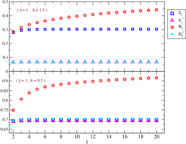
Figure 4: (color online)Comparision of the (truncated) Shannon entropy $(H^{t}_{1})H_{1}$ with the (truncated) von Neumann entropy $(S^{t}_{1})S_{1}$ for two gapped points $(\gamma,h)=(1,\frac{1}{2})$ and $(\gamma,h)=(1,\frac{3}{2})$.

IV.2 Rényi entanglement entropy and Rényi entropy of the subsystem energy

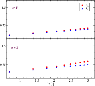
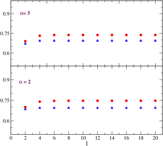
Figure 5: (color online) Comparing the entanglement entropy and the Rényi entropy of the subsystem energy for $\alpha=2$ and $5$. Top: Critical XY chain $(\gamma=1,h=1)$. In this case, to better verify the closeness, we have depicted the entropies in the semi-log plots which indicates that for bigger $\alpha$’s, they become closer. Bottom: Non-critical XY chain $(\gamma=1,h=0.5)$.

In this subsection, we provide some numerical results to support our claims on the closeness of the Rényi entanglement entropy and the Rényi entropy of the subsystem energy. There are at least a couple of different ways to investigate this matter. The first and more direct one is to compare the two entropies for different $\alpha$’s. In the Figure 5, we have depicted the two entropies, $H_{\alpha}$ and $S_{\alpha}$ with respect to $l$ (the size of the subsystem for the critical Ising model) for various values of $\alpha=2$ and $5$. It is clear that for bigger $\alpha$’s, the two entropies mimic each other closely. Similar conclusions are also valid for the other critical systems. We have done similar calculations for the non-critical ground states as well and the result is shown in the Figure 5. The conclusions are similar which support the closeness of the Rényi entropy of the subsystem energy to the Rényi entanglement entropy. Since for the bigger $\alpha$’s the convergence is better ( even for the small sites considered here), one immediately guesses that the closeness of the Rényi entropy of the subsystem energy to the Rényi entanglement entropy might be due to the closeness of the biggest probabilities to the largest eigenvalues of the reduced density matrix. To verify this argument, we directly compare the two sets of numbers as the second method to see the similarity between these two quantities. In the Figure 6, we numerically showed that this is actually true. In other words, at least, the two biggest probabilities, i.e. $P_{g}$ and $P_{1}$, closely follow the two biggest eigenvalues of the reduced density matrix, i.e. $\lambda_{\text{max}}$ and $\lambda_{1}$. Furthermore, we have checked numerically in many other points of the phase diagram and observed the same behavior. It might be interesting to investigate the connection of these conclusions to the behavior of the Schmidt gap under the phase transition studied recently in DeChiara2012 ; Bayat2014 .

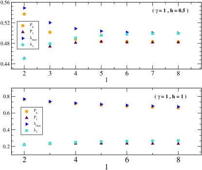
Figure 6: (color online) Comparing the two biggest probabilities in the subsystem energy basis indicated as $P_{g}$ and $P_{1}$ with the two biggest eigenvalues of the reduced density matrix, indicated with $\lambda_{max}$ and $\lambda_{1}$. Both for the critical $(\gamma=1,h=1)$ and the noncritical case $(\gamma=1,h=0.5)$ depicted in the bottom and the top respectively. The $P_{g}$ closely mimics $\lambda_{max}$ while $P_{1}$ mimics the $\lambda_{1}$.

Finally, we have also investigated the closeness of the two entropies for small sizes. In the Figure 7, we illustrate the $H_{\alpha}$ and $S_{\alpha}$ as a function of $\alpha$ for $L=2$ and $L=4$ at both the critical and the non-critical points. It is clear that even for small sizes, the Rényi entropy of the subsystem energy chases the Rényi entanglement entropy and becomes incredibly close for bigger values of $\alpha$ as we mentioned earlier.

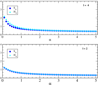
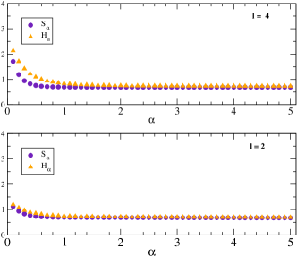
Figure 7: (color online) Comparing the two entropies $H_{\alpha}$ and $S_{\alpha}$ with respect to $\alpha$ for small sizes $l=2$ and $l=4$ at the critical Ising point $(\gamma=1,h=1)$ depicted in the top and the noncritical point $(\gamma=1,h=0.5)$ depicted in the bottom panel. For both cases and for both of the sizes, we observe that the Rényi entropy of the subsystem energy behave similarly to the Rényi entanglement entropy and they get closer for bigger values of $\alpha$.

IV.3 Schmidt basis and the truncated Hamiltonian basis

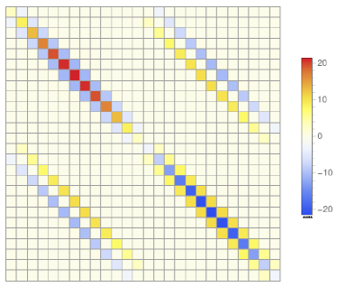
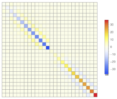
Figure 8: (color online) Comparing matrices $\begin{pmatrix}\textbf{M}&\textbf{N}\\ -\textbf{N}&-\textbf{M}\\ \end{pmatrix}$ illustrated in the top and $\textbf{Q}=\textbf{U}\begin{pmatrix}\textbf{M}&\textbf{N}\\ -\textbf{N}&-\textbf{M}\\ \end{pmatrix}\textbf{U}^{\dagger}$ illustrated in the bottom for a subsystem with size $l=13$. Notice that both matrices are block matrices of size $2l$ and the majority of the matrix elements are nearly zero. Although there are some nonzero values in the diagonal part of the matrix N which manifest itself in the upper right and lower left diagonal of the matrix in the bottom panel, it is remarkable that after rewriting it in the truncated Hamiltonian basis, those elements nearly vanish and the result matrix Q becomes an almost diagonal matrix.

Here, we study the difference between the Schmidt basis and the truncated Hamiltonian basis. To this end, we compare the reduced density matrix written in these two bases and show that they are close to each other in the sense of norm distance. The reduced density matrix in the truncated Hamiltonian basis as we discussed in section III, has the following form

$$\rho=\det\frac{1}{2}(\mathbb{I}-\textbf{G})[{\rm\det}(\textbf{F}_{s})]^{\frac{1}{2}}e^{\frac{1}{2}(\boldsymbol{\eta}^{\dagger}\,\,\boldsymbol{\eta})\textbf{Q}\begin{pmatrix}\boldsymbol{\eta}\\ \boldsymbol{\eta}^{\dagger}\\ \end{pmatrix}}.$$ (34)

Note that here, we use the word basis in the sense of writing the density matrix with respect to the proper creation-annihilation operators. The reason will be clear in few lines. However, in the Schmidt basis, it has the following form

$$\rho=\det\frac{1}{2}(\mathbb{I}-\textbf{G})[{\rm\det}(\textbf{F}_{s})]^{\frac{1}{2}}e^{\frac{1}{2}(\boldsymbol{\delta}^{\dagger}\,\,\boldsymbol{\delta})\textbf{D}\begin{pmatrix}\boldsymbol{\delta}\\ \boldsymbol{\delta}^{\dagger}\\ \end{pmatrix}},$$ (35)

where D is a diagonal matrix. The above two density operators written in the current form are the same density operators written with respect to the different creation-annihilation operators. Note that by diagonalizing the Q, we reach to the matrix D. Clearly, if the Q was diagonal, then, the two bases were equal. However, as a remarkable result, the matrix Q becomes close to diagonal. In Figure 8, we have depicted the $\begin{pmatrix}\textbf{M}&\textbf{N}\\ -\textbf{N}&-\textbf{M}\\ \end{pmatrix}$ and $\textbf{Q}=\textbf{U}\begin{pmatrix}\textbf{M}&\textbf{N}\\ -\textbf{N}&-\textbf{M}\\ \end{pmatrix}\textbf{U}^{\dagger}$ for the subsystem with the size $l=13$. Comparing these two matrices, it is striking that the $\rho_{D}$ written in the truncated Hamiltonian becomes near diagonal as the off-diagonal elements washed out in this new basis.

To quantify the difference between the two bases at the level of the density matrices, we first consider that the $\eta$ is equal to $\delta$ in the equation (34) and write

$$\rho_{e}=\det\frac{1}{2}(\mathbb{I}-\textbf{G})[{\rm\det}(\textbf{F}_{s})]^{\frac{1}{2}}e^{\frac{1}{2}(\boldsymbol{\delta}^{\dagger}\,\,\boldsymbol{\delta})\textbf{Q}\begin{pmatrix}\boldsymbol{\delta}\\ \boldsymbol{\delta}^{\dagger}\\ \end{pmatrix}},$$ (36)

and consequently, for the Schmidt basis, we write

$$\rho_{s}=\det\frac{1}{2}(\mathbb{I}-\textbf{G})[{\rm\det}(\textbf{F}_{s})]^{\frac{1}{2}}e^{\frac{1}{2}(\boldsymbol{\delta}^{\dagger}\,\,\boldsymbol{\delta})\textbf{D}\begin{pmatrix}\boldsymbol{\delta}\\ \boldsymbol{\delta}^{\dagger}\\ \end{pmatrix}}.$$ (37)

Obviously, the above two density matrices are not the same density matrices and one may find their distance by looking at the Frobenius norm distance defined as follows:

$$||\rho_{e}-\rho_{s}||_{{}_{F}}=(\text{tr}[\rho_{e}-\rho_{s}]^{2})^{\frac{1}{2}}.$$ (38)

This quantity is a measure of the distance between the density matrices written in the two different bases and can be easily calculated for our density matrices using the following formulas

$$\text{tr}\rho_{s}^{2}=\text{tr}\rho_{e}^{2}=\det\frac{1}{2}(\mathbb{I}-\textbf{G})[{\rm\det}(\textbf{F}_{s})]^{\frac{1}{2}}\prod_{i=1}^{l}(2\cosh\lambda^{Q}_{i}),$$

$$\text{tr}[\rho_{s}\rho_{e}]=\det\frac{1}{2}(\mathbb{I}-\textbf{G})[{\rm\det}(\textbf{F}_{s})]^{\frac{1}{2}}\prod_{i=1}^{l}(2\cosh\frac{\lambda^{\tilde{Q}_{i}}}{2}),$$

where $\lambda^{Q}_{i}$’s are the positive eigenvalues of the matrix Q and $\lambda^{\tilde{Q}}_{i}$’s are the positive eigenvalues of the matrix $\tilde{\textbf{Q}}$ defined as $e^{\tilde{\textbf{Q}}}=e^{\textbf{Q}}e^{\textbf{D}}$.

To have a measure of how big is the Frobenius distance, we compare it with the Frobenius norm of the density matrix itself and define

$$r=\frac{||\rho_{e}-\rho_{s}||_{{}_{F}}}{||\rho_{s}||_{{}_{F}}}$$ (40)

In the Figure 9, we depicted this ratio for different points on the phase diagram of the XY chain for different subsystem sizes. The ratio is always smaller than one and saturates for larger subsystem sizes which indicates that the two bases are not far from each other. Note that for two arbitrary density matrices the ratio is normally bigger than one. For example, we realized that this ratio is around one if one shuffles the order of the eigenvalues of the matrix D.

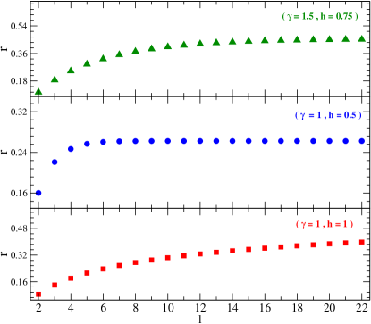
Figure 9: (color online) The norm ratio for different points in the phase diagram of the XY chain. As it is shown in the different panels, for all of the cases the norm riches a constant value which is smaller than one. For the case of the critical point depicted in the bottom panel, the convergence is slower as one might be expected.

V Rényi entropy of the subsystem energy and the Loschmidt echo

It is possible to connect the generating function of our quantity, i.e. $M(z)=\text{tr}[\rho_{l}e^{zH_{l}}]$, to the fidelity amplitude by first preparing the full system in the ground state and then turning off the couplings between the Hamiltonian of the subsystem with the rest of the system and also, switching off all the couplings between the spins outside of the subsystem. The current Hamiltonian is now $H_{l}\otimes I_{\bar{l}}$. The we can calculate the Loschmidt amplitude in the Schmidt basis, i.e. $|\psi_{g}\rangle=\sum_{j}\lambda_{j}|\phi^{(l)}_{j}\rangle\otimes|\phi^{(\bar{l})}_{j}\rangle$

$$\langle\psi_{g}|e^{-it(H_{l}\otimes I_{\bar{l}})}|\psi_{g}\rangle = \sum_{j,k}\lambda_{j}\lambda_{k}\langle\phi^{(l)}_{j}|e^{-itH_{l}}|\phi_{k}^{(l)}\rangle\delta_{jk}$$ (41)

$$= \sum_{j}\lambda_{j}^{2}\langle\phi^{(l)}_{j}|e^{-itH_{l}}|\phi_{j}^{(l)}\rangle$$

This quantity is nothing except $\text{tr}[\rho_{l}e^{-itH_{l}}]$ which leads to

$$M(-it)=\langle\psi_{g}|e^{-it(H_{l}\otimes I_{\bar{l}})}|\psi_{g}\rangle$$ (42)

Using the above equation, we end up with a remarkable result that one can generate the probability distribution of finding the system in different energy states by just performing an inverse Fourier transform. In other words

$$P(E_{j})=\frac{1}{2\pi}\int dte^{itE_{j}}M(-it)$$ (43)

Using the above probabilities one can calculate the desired entropies. Notice that the right hand side in equation (43) is the Loschmidt amplitude and remarkably, the inverse Fourier transform of this amplitude gives us the desired probability distributions. Finally, there is a number of different experiments which make the measurement of the Loschmidt amplitude possible. In a recent experiment, the time resolved state tomography provided a full access to the evolution of the wavefunction in ultracold atoms Flaschner2016 ; Flaschner2018 . In another directly related experiment, an efficient MPS tomography for the XY model has been used to reconstruct the full density matrix for the short range interaction which enables one to measure the Loschmidt amplitude Roos2017 ; Cramer2010 . Furthermore, there is relatively an easier method to measure $H_{2}$ as it is related to the Loschmidt probabilities which has been measured in a recent experiment of 1D trapped ions Jurcevic2017 . We note that our proposal is reminiscent of the recent measurement quench protocolJurcevic2015 ; Bayat2018

VI Conclusions

In this paper, we showed that the subsystem energy entropy is an excellent quantity which can mimic the entanglement entropy of many body systems at and off the critical point. For the non-critical systems, the defined Rényi entropy for sufficiently large $\alpha$’s follows an area law and at the critical point it follows a logarithmic behavior with a universal coefficient. It can be used to detect the phase transition and determine the universality class. We also proposed an experimental setup to measure our quantity with the current technology. Since the probabilities introduced in this paper follow closely the Schmidt coefficients our protocol can be used to measure the Schmidt coefficients effectively. For example, for the gapped systems the few largest probabilities are extreemly close to the biggest Schmidt coefficients. In another words finding the first largest probabilities provide an approximation for the most relevant Schmidt coefficients. It would be very important to calculate this quantity in QFT (CFT) to have a better idea about the nature of the universality of the presented results bosonic . The recent developments regarding the distribution of the energy-momentum tensor in QFT(CFT) might be very useful, see Ref. Fewster2018 and references therein.

Acknowledgement We thank P Calabrese, M. Collura and N. M. Linke for discussions. We thank E. Barnes for reading the manuscript and his useful comments. The work of MAR was supported in part by CNPq. The work of K.N. is supported by National Science Foundation under Grant No. PHY-1620555 and DOE grant DE-SC0018326.

Appendix A Diagonalization of the Free Fermions

In this subsection, we summarize the result of Ref.LSM . Consider a generic (real) truncated free fermion Hamiltonian defined in domain $D$:

$$\ \textbf{H}_{D}=\sum_{ij}[c_{i}^{\dagger}A_{ij}c_{j}+\frac{1}{2}c_{i}^{\dagger}B_{ij}c_{j}^{\dagger}+\frac{1}{2}c_{i}B_{ji}c_{j}]-\frac{1}{2}{\rm Tr}{\textbf{A}},\hskip 28.45274pt$$ (44)

where $c_{i}^{\dagger}$ and $c_{i}$ are fermionic creation and annihilation operators and $i=1,2,...,|D|$, where $|D|$ is the number of sites in the region $D$. The Hermitian Hamiltonian requires A and B to be symmetric and antisymmetric matrices respectively. To diagonalize the Hamiltonian we use the following canonical transformation

$$\ \begin{pmatrix}\textbf{c}\\ \textbf{c}^{\dagger}\\ \end{pmatrix}=\textbf{U}^{\dagger}\begin{pmatrix}\boldsymbol{\eta}\\ \boldsymbol{\eta}^{\dagger}\\ \end{pmatrix},$$ (45)

with

$$\ \textbf{U}=\begin{pmatrix}\textbf{g}&\textbf{h}\\ \textbf{h}^{*}&\textbf{g}^{*}\\ \end{pmatrix}.$$ (46)

Then, we can write the diagonalized from of the Hamiltonian as follows

$$\ \textbf{H}_{D}=\sum_{k}|\lambda_{k}|(\eta_{k}^{\dagger}\eta_{k}-\frac{1}{2}).$$ (47)

Note that g and h can be derived from the following equations:

g $$= \frac{1}{2}(\boldsymbol{\phi}+\boldsymbol{\psi}),$$ (48)

h $$= \frac{1}{2}(\boldsymbol{\phi}-\boldsymbol{\psi}),$$ (49)

where we have

$$\ (\textbf{A}+\textbf{B})\phi_{k} = |\lambda_{k}|\psi_{k},$$ (50)

$$(\textbf{A}-\textbf{B})\psi_{k} = |\lambda_{k}|\phi_{k},$$ (51)

or

$$\ (\textbf{A}-\textbf{B})(\textbf{A}+\textbf{B})\phi_{k} = |\lambda_{k}|^{2}\phi_{k},$$ (52)

$$(\textbf{A}+\textbf{B})(\textbf{A}-\textbf{B})\psi_{k} = |\lambda_{k}|^{2}\psi_{k}.$$ (53)

When $\lambda_{k}\neq 0$, $\phi_{k}$ and $\lambda_{k}$ can be calculated by solving the eigenvalue equation (52), then, $\psi_{k}$ can be determined using (50). When $\lambda_{k}=0$, $\phi_{k}$ and $\psi_{k}$ can be deduced directly from (50) and (51).

The correlation matrix G for the full system defined as

$$G_{ij} = \langle(c_{i}^{\dagger}-c_{i})(c_{j}^{\dagger}+c_{j})\rangle$$ (54)

can be also calculated using the above procedure as follows:

$$\textbf{G}=(\hat{\textbf{h}}^{\dagger}-\hat{\textbf{g}}^{\dagger})(\hat{\textbf{g}}+\hat{\textbf{h}}).$$ (55)

Note that in the above equation we put hat on the g and h matrices to emphasize that one should calculate them using the $\hat{\textbf{A}}$ and $\hat{\textbf{B}}$ matrices. Since we never calculate the correlation matrix for the truncated Hamiltonian we do not put hat on this matrix.

Appendix B Generating function of the subsystem energy

It is worth mentioning that the results of this section can be used to get also an explicit formula for the generating function of the subsystem energy. Different versions of this quantity are already appeared in Najafi2017 . We present here another version which has different form but it is equivalent to the previous ones. The generating function is defined as:

$$M(z)=\text{tr}[\rho_{D}e^{z\textbf{H}_{D}}].$$ (56)

After writing $\textbf{H}_{D}$ as

$$\textbf{H}_{D}=\frac{1}{2}(\textbf{c}^{\dagger}\,\,\textbf{c})\begin{pmatrix}\textbf{A}&\textbf{B}\\ -\textbf{B}&-\textbf{A}\\ \end{pmatrix}\begin{pmatrix}\textbf{c}\\ \textbf{c}^{\dagger}\\ \end{pmatrix}$$ (57)

and using (12) the trace can be calculated explicitly. The final result is

$$M(z)=\det\frac{1}{2}(\mathbb{I}-\textbf{G})[{\rm\det}(\textbf{F}_{s})]^{\frac{1}{2}}\det[\mathbb{I}+e^{z\begin{pmatrix}\textbf{A}&\textbf{B}\\ -\textbf{B}&-\textbf{A}\\ \end{pmatrix}}e^{\begin{pmatrix}\textbf{M}&\textbf{N}\\ -\textbf{N}&-\textbf{M}\\ \end{pmatrix}}]^{\frac{1}{2}}.$$ (58)

The above equation can be also written as

$$M(z)= \det\frac{1}{2}(\mathbb{I}-\textbf{G})[{\rm\det}(\textbf{F}_{s})]^{\frac{1}{2}}$$ (59)

$$\times\det[\mathbb{I}+\begin{pmatrix}e^{z|\boldsymbol{\lambda}|}&0\\ 0&e^{-z|\boldsymbol{\lambda}|}\\ \end{pmatrix}\tilde{\textbf{T}}]^{\frac{1}{2}};\hskip 28.45274pt$$

where $|\boldsymbol{\lambda}|$ is the matrix of the eigenvalues of the subsystem Hamiltonian. Since the involved matrices normally does not have simple properties it seems difficult to find the analytical properties of the above formula for large subsystem sizes.

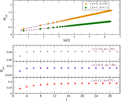
Figure 10: (color online)Up: logarithmic behavior of the Rényi entropy ($\alpha\to\infty$) of the subsystem energy of the critical XY chain for $\gamma=h=0$ and $\gamma=h=1$. Down: area law of the Rényi entropy ($\alpha\to\infty$) for various values of the parameters of the gapped XY chain.

Appendix C Further Numerical Details

In this section, we will summarize further numerical results regarding the Rényi entropy of the subsystem energy. We will mostly focus on the $\alpha\to\infty$ where we can work with the biggest probability. In this case, we can calculate the entropy for relatively large subsystem sizes with high accuracy. For example, in Fig. 10, we checked the area law for the gapped phase with much more accuracy. Then, in the table I and II we show the universality of the coefficient of the logarithm, i. e. $\epsilon(\infty)$, in the critical regime for the critical XY line and the XX line respectively. In the same tables one can also see that the coefficient corresponding to the semi-infinite case $\epsilon_{s}(\infty)$ is half of the infinite case. This is exactly what happens for the entanglement entropyCC2004 . Note that the coefficients of the critical Ising universality is with high accuracy half of the the XX universality. This indicates that most probably the coefficients $\epsilon(\infty)$ and $\epsilon_{s}(\infty)$ are linearly proportional to the central charge of the underlying CFT.

$(h,\gamma)$	$\epsilon(\infty)$	$\epsilon_{s}(\infty)$
$(1,1)$	$0.111(1)$	$0.055(1)$
$(1,0.5)$	$0.111(1)$	$0.055(1)$
$(1,0.75)$	$0.111(1)$	$0.055(1)$
$(1,1.25)$	$0.111(1)$	$0.055(1)$
$(1,1.5)$	$0.111(1)$	$0.055(1)$

Table 1: The coefficients $\epsilon(\infty)$ and $\epsilon_{s}(\infty)$ for various $\gamma$’s on the critical XY line.

$n_{c}$	$\epsilon(\infty)$	$\epsilon_{s}(\infty)$
$\pi/2$	$0.222(2)$	$0.111(2)$
$14\pi/30$	$0.222(2)$	$0.111(2)$
$9\pi/20$	$0.222(2)$	$0.111(2)$
$8\pi/18$	$0.222(2)$	$0.111(2)$
$7\pi/16$	$0.222(2)$	$0.111(2)$
$6\pi/14$	$0.222(2)$	$0.111(2)$
$5\pi/12$	$0.222(2)$	$0.111(2)$
$4\pi/10$	$0.223(2)$	$0.111(2)$
$3\pi/8$	$0.224(2)$	$0.112(2)$
$\pi/3$	$0.225(2)$	$0.112(2)$

Table 2: The coefficients $\epsilon(\infty)$ and $\epsilon_{s}(\infty)$ for various values of the fillings $h=-2\cos n_{c}$ on the critical XX line, i.e. $\gamma=0$.

References

- (1) L. Amico, R. Fazio, A. Osterloh, and V. Vedral, Rev. Mod. Phys. 80, 517 (2008).
- (2) I. Affleck, N. Laflorencie and E. S. Sørensen, J. Phys. A: Math. Theor. 42, 504009 (2009).
- (3) G. Refael, J. E. Moore, J. Phys. A: Math. Theor. 42, 504010 (2009).
- (4) I. Peschel and V. Eisler, J. Phys. A: Math. Theor. 42 (50), 504003 (2009).
- (5) J. Eisert, M. Cramer and M. B. Plenio, Rev. Mod. Phys. 82, 277 (2010).
- (6) K. Modi, A. Brodutch, H. Cable, T. Paterek, and V. Vedral, Rev. Mod. Phys. 84, 1655 (2012).
- (7) N. Laflorencie, Phys. Rept. 646, 1–59, (2016).
- (8) G. De Chiara, A. Sanpera, arXiv:1711.07824.
- (9) P. Calabrese, J. Cardy, J. Phys. A 42, 504005 (2009).
- (10) O. A. Castro-Alvaredo, B. Doyon, J. Phys. A 42, 504006 (2009).
- (11) H. Casini and M. Huerta, J. Phys. A. 42, 504007 (2009).
- (12) M. Rangamani, and T. Takayanagi, Lect. Notes Phys. 931, 1–246 (2017).
- (13) T. Nishioka, arXiv:1801.10352.
- (14) P. J. Coles, M. Berta, M. Tomamichel, and S. Wehner, Rev. Mod. Phys. 89, 015002 (2017).
- (15) J.-M. Stéphan, G. Misguich, and V. Pasquier, Phys. Rev. B 82, 125455 (2010).
- (16) J.-Marie Stéphan, G. Misguich, and V. Pasquier, Phys. Rev. B 84, 195128 (2011).
- (17) E. Fradkin and J. E. Moore, Phys. Rev. Lett. 97, 050404 (2006).
- (18) G. Misguich, V. Pasquier, M. Oshikawa, Phys. Rev. B 95, 195161 (2017).
- (19) J-M Stéphan, J. Stat. Mech. P05010 (2014).
- (20) M. A. Rajabpour, EPL. 112, 66001 (2015).
- (21) K. Najafi and M. A. Rajabpour, Phys. Rev. B 93, 125139 (2016).
- (22) M. A. Rajabpour, J. Stat. Mech. 123101 (2016).
- (23) The volume law simply reflects that the state spreads over exponential number of configurations.
- (24) F. C. Alcaraz, M. A. Rajabpour, Phys. Rev. Lett. 111, 017201 (2013).
- (25) J-M Stéphan, Phys. Rev. B 90, 045424 (2014).
- (26) F. C. Alcaraz, M. A. Rajabpour, Phys. Rev. B 90, 075132 (2014).
- (27) F. C. Alcaraz, M. A. Rajabpour, Phys. Rev. B 91, 155122 (2015).
- (28) F. C. Alcaraz, Phys. Rev. B 94, 115116 (2016).
- (29) D. J. Luitz, F. Alet, N. Laflorencie, Phys. Rev. Lett. 112, 057203 (2014).
- (30) D. J. Luitz, F. Alet, N. Laflorencie, Phys. Rev. B 89, 165106 (2014).
- (31) D. J. Luitz, N. Laflorencie, F. Alet, J. Stat. Mech. P08007 (2014).
- (32) M. M. Wilde, Quantum Information Theory (Cambridge University Press, Cambridge, England, 2013).
- (33) M. B. Hastings, J. Stat. Mech. 08, P08024 (2007).
- (34) F. G. S. L. Brandao, M. Horodecki, Nature Physics 9, 721 (2013).
- (35) I. Arad, Z. Landau, and U. Vazirani. Phys. Rev. B 85, 195145 (2012).
- (36) F. G. S. L. Brandao, M. Horodecki, Comm. Math. Phys. 333, 761 (2015).
- (37) C. Holzhey, F. Larsen, and F. Wilczek, Nucl. Phys. B 424, 443 (1994).
- (38) G. Vidal, J. I. Latorre, E. Rico, and A. Kitaev, Phys. Rev. Lett. 90, 227902 (2003).
- (39) P. Calabrese and J. Cardy, J. Stat. Mech. P06002 (2004).
- (40) V. Eisler, Z. Rácz, and F. van Wijland, Phys. Rev. E67, 056129 (2003).R. W. Cherng and E. Demler, New J. Phys. 9, 7 (2007).
- (41) I. Klich, G. Refael, and A. Silva, Phys. Rev. A 74, 32306 (2006).
- (42) I. Klich and L. Levitov, Phys. Rev. Lett. 102, 100502 (2009).
- (43) P. Calabrese, M. Mintchev, E. Vicari, EPL. 98, 20003 (2012).
- (44) H. F. Song, S. Rachel, C. Flindt, I. Klich, N. Laflorencie, and K. Le Hur, Phys. Rev. B 85, 035409 (2012).
- (45) S. Rachel, N. Laflorencie, H. F. Song, and K. Le Hur, Phys. Rev. Lett. 108, 116401 (2012).
- (46) I. Klich, J. Stat. Mech. P11006 (2014).
- (47) M. Collura, F. H. L. Essler, and S. Groha, J. Phys. A: Math. Theor. 50 414002 (2017); J.-M. Stéphan, F. Pollmann, Phys. Rev. B 95, 035119 (2017); A. Bastianello, L. Piroli, and P. Calabrese, Phys. Rev. Lett. 120 (19), 190601; S. Groha, F. H. L. Essler, P. Calabrese, arXiv1803.09755 and J. C. Xavier, F. C. Alcaraz, G. Sierra, arXiv:1804.06357.
- (48) A. Lamacraft, P. Fendley, Phys. Rev. Lett. 100, 165706 (2008).
- (49) K. Najafi and M. A. Rajabpour, Phys. Rev. B 96, 235109 (2017).
- (50) The generalization to short-range interacting systems, finite systems and also higher dimensions is trivial.
- (51) M. Müller, E. Adlam, L. Masanes, and N. Wiebe, Commun. Math. Phys. 340, 499–561 (2015).
- (52) I. Arad, T. Kuwahara, Z. Landau, J. Stat. Mech. 33301 (2016).
- (53) The precise statement of the theorom is the following: consider an arbitrary eigenstate of the total Hamiltonian and a sub-region with complement . Define where is a region around which the boundary terms of the sites inside interact. Then, the theorem tells us that there is a density matrix in which is weakly diagonal in the eigenbasis of and satisfies . Here, the weekly diagonal means that for two different eigenvectors of the Hamiltonian , we have , where and are constants.
- (54) In principle to calculate the full distribution one might first try to calculate the generating function of the subsystem energy distribution as it was done in Najafi2017 , see Appendix B. Different explicit determinant formulas can be calculated for the generating functions but their forms are normally too complicated to be useful to calculate the probability distributions for large sizes numerically.
- (55) M. C. Chung and I. Peschel, Phys. Rev. B 64, 064412 (2001) and I. Peschel, J. Phys. A: Math. Gen. 36, L205 (2003).
- (56) T. Barthel, M-C. Chung, U. Schollwöeck, Phys. Rev. A 74, 022329 (2006).
- (57) R. Balian and E. Brézin, Nuov. Cim. 64 B 37 (1969).
- (58) E. Lieb, T. Schultz, and D. Mattis, Annals of Physics 16, 407 (1961).
- (59) Unfortunately we realized that it is difficlut to calculate effectively. For example, although is for sure smaller than two with the current limitations in our numerical calculations, it is not clear our conclusion can be applied to also the Shannon entropy for the generic values of and .
- (60) For example, we checked that the smallest probability which corresponds to the highest energy decays supper-exponentially with the subsystem size, i.e. . We believe that the same is true for majority of states with high energies which makes their contribution to the Shannon entropy negligible. One might also understand the absence of the volume-law based on the same line of argument.
- (61) J. Dubail, J-M Stéphan, J. Stat. Mech. L03002 (2011).
- (62) J. Dubail, J-M Stéphan, J. Stat. Mech. P09002 (2013).
- (63) Here we truncate the number of probabilities at when () is less than percent of ().
- (64) Similarly one can also define a truncated Rényi entropy. Our conclusions are also valid in this case too.
- (65) We believe that effectiveness of just taking one(two) probabilities is a property of the XY chain. In other models the number of needed probabilities might vary depending on the symmetries of the system but it will not scale with the size of the subsystem.
- (66) G. De Chiara, L. Lepori, M. Lewenstein, and A. Sanpera, Phys. Rev. Lett. 109, 237208 (2012).
- (67) A. Bayat, H. Johannesson, S. Bose and P. Sodano, Nat. Comm. 5, 3784 (2014).
- (68) N. Fläschner, B. S. Rem, M.Tarnowski, D. Vogel, D. S. Lühmann, K. Sengstock and C. Weitenberg, Science 352 1091(2016).
- (69) N. Fläschner, D. Vogel, M. Tarnowski, B. S. Rem, D. S. Lühmann, M. Heyl, J. C. Budich, L. Mathey, K. Sengstock, C. Weitenberg, Nat. Phys. 14, 265 (2018).
- (70) B. P. Lanyon, C. Maier, M. Holzäpfel, T. Baumgratz, C. Hempel, P. Jurcevic, I. Dhand, A. S. Buyskikh, A. J. Daley, M. Cramer, M. B. Plenio, R. Blatt and C. F. Roos, Nat. Phys. 13 (2017).
- (71) M. Cramer, M. B. Plenio, S.T. Flammia, D. Gross, S. D. Bartlett, R. Somma, O. L. Cardinal, Yi-Kai Liu, D. Poulin, Nat. Commun. 1, 149 (2010).
- (72) P. Jurcevic, H. Shen, P. Hauke, C. Maier, T. Brydges, C. Hempel, B. P. Lanyon, M. Heyl, R. Blatt, C. F. Roos, Phys. Rev. Lett. 119, 080501 (2017).
- (73) P. Jurcevic, P. Hauke, C. Maier, C. Hempel, B. P. Lanyon, R. Blatt, C. F. Roos, Physical review letters 115 (10), 100501 (2015).
- (74) A. Bayat, B. Alkurtass, P. Sodano, H. Johannesson, and S. Bose Phys. Rev. Lett. 121, 030601 (2018)
- (75) C. J. Fewster, S. Hollands, arXiv:1805.04281.
- (76) The bosonic systems, especially coupled harmonic oscillators will be studied in an other work.