On the approaching time towards the attractor of differential equations perturbed by small noise

Abstract

We estimate the time a point or set, respectively, requires to approach the attractor of a radially symmetric gradient type stochastic differential equation driven by small noise. Here, both of these times tend to infinity as the noise gets small. However, the rates at which they go to infinity differ significantly. In the case of a set approaching the attractor, we use large deviation techniques to show that this time increases exponentially. In the case of a point approaching the attractor, we apply a time change and compare the accelerated process to another process and obtain that this time increases merely linearly.

Keywords. random attractor, stochastic differential equation, synchronization, large deviation principle
2010 Mathematics Subject Classification. 37G35, 37H99, 60F10, 60H10

1 Introduction

Noise induced stabilization is an interesting phenomena to occur. Here, the long-time dynamics in the absence of noise are not asymptotically stable while the addition of noise stabilizes the dynamics. One way to quantify the asymptotic behavior is to analyze (random) attractors. The most common kinds of (random) attractors are (random) point and set attractors. While (random) point attractors need to attract any single point, (random) set attractors even need to attract compact sets uniformly. If an (random) attractor is a single (random) point, the long-time dynamics are asymptotically globally stable.
In the case of noise induced stabilization, we can anticipate that the time required for a point or set, respectively, to approach the attractor goes to infinity as the noise, which stabilizes the system, gets small. Our aim is to estimates these times and provide the rates at which they tend to infinity.
We consider a radially symmetric gradient type stochastic differential equation, i.e.

$$dX_{t}^{\varepsilon}=-\nabla U(X_{t}^{\varepsilon})dt+\sqrt{\varepsilon}dW_{t}\quad\textrm{on }\mathbb{R}^{d}$$ (1)

where $d\geq 2$, $\varepsilon>0$, $W_{t}$ is a $d$-dimensional Brownian motion and $U(x)=u(|x|^{2})$ for all $x\in\mathbb{R}^{d}$ and some twice differentiable convex function $u:[0,\infty)\rightarrow\mathbb{R}$ attaining its unique minimum in $(0,\infty)$.
In the absence of noise, the solution of the differential equation

$$dx_{t}=-\nabla U(x_{t})dt\qquad\textrm{on }\mathbb{R}^{d}.$$ (2)

has a stable sphere, meaning that any point on this sphere is a fixed point and any point except $0$ converges towards the sphere under the dynamics of (2). The point $0$ is also a fixed point. In terms of attractors this means that the point attractor is the union of $0$ and the stable sphere while the set attractor is the closed ball of the same radius as the stable sphere centered at $0$.
An interesting phenomena occurs if one adds noise as in (1). In [7] it was shown that under some general conditions on $U$, the attractor of (1) collapses to a single random point. Therefore, the addition of noise stabilizes the system. This phenomenon is called synchronization by noise.
The question that arises is how fast this phenomena occurs for small noise. By the above observations it is obvious that the time until a point or a set, respectively, approaches the attractor should go to infinity as the noise gets small. We estimate the rates at which these times tend to infinity and even show a significant difference between the time a point or a set, respectively, requires to approach the attractor. This difference is due to the fact that a point can approach the attractor moving to the stable sphere and then along the sphere while a set can just approach the attractor if a point of the stable sphere moves close to zero.
In section 3, we show that the time until a set approaches the attractor increases exponentially in $\varepsilon^{-1}$ using large deviation techniques similar to [5, Section 5.7]. We obtain a lower bound by taking the difference of the potential describing the costs of a point on the stable sphere to approach zero. Assuming that the differential equation (2) pushes all mass into a bounded set in finite time, we get a upper bound for the time. This estimate in particular demonstrates the sharpness of our lower bound.
In section 4, we prove that the time until a point approaches the attractor is of order $\varepsilon^{-1}$ for dimension $d=2$. Here, we accelerate the process and compare the accelerated process to a process on the sphere that is known to synchronize weakly.

2 Preliminaries

We consider the stochastic differential equation (SDE) (1) and assume that $-\nabla U$ satisfies a one-sided-Lipschitz condition, i.e. there exists some $C>0$ such that

$$\langle x-y,-\nabla U(x)+\nabla U(y)\rangle\leq C|x-y|^{2}$$

for all $x,y\in\mathbb{R}^{d}$. Then, the SDE (1) has a unique solution. We denote by $X^{\varepsilon}:[0,\infty)\times\Omega\times\mathbb{R}^{d}\rightarrow\mathbb{R}^{d}$ the solution of (1).
We say that the SDE (1) is strongly contracting if there exist $r,t>0$ such that $|x_{t}(y)|\leq r$ for all $y\in\mathbb{R}^{d}$ where $x_{t}(y)$ is the solution of the deterministic differential equation started in $y$. Therefore, the SDE (1) is strongly contracting if and only if $\int_{R}^{\infty}|\nabla U(x)|^{-1}dx$ exists for some $R>0$.
Let $R^{\ast}\in(0,\infty)$ be the point where $u$ attains its minimum, i.e. $u(R^{\ast})<u(x)$ for any $x\not=R^{\ast}$. We restrict the proofs in the following sections to the case $R^{\ast}=1$. However, all results are extendable to general $R^{\ast}\in(0,\infty)$ since $X_{t}^{\varepsilon}/R^{\ast}$ is of the postulated form.
Attractors and synchronization are defined for random dynamical systems. We restrict our definitions to a random dynamical system on $\mathbb{R}^{d}$, see [1] for a more general setting.

Definition 2.1 (Metric Dynamical System).

Let $(\Omega,\mathcal{F},\mathbb{P})$ be a probability space and $\theta=(\theta_{t})_{t\in\mathbb{R}}$ be a group of maps $\theta_{t}:\Omega\rightarrow\Omega$ satisfying

1. $(\omega,t)\mapsto\theta_{t}(\omega)$ is $(\mathcal{F}\otimes\mathcal{B}(\mathbb{R}),\mathcal{F})$-measurable,

2. $\theta_{0}(\omega)=\omega$ for all $\omega\in\Omega$,

3. $\theta_{s+t}=\theta_{s}\circ\theta_{t}$ for all $s,t\in\mathbb{R}$,

4. $\theta_{t}$ has ergodic invariant measure $\mathbb{P}$.

The collection $(\Omega,\mathcal{F},\mathbb{P},\theta)$ is then called a metric dynamical system.

Definition 2.2 (Random Dynamical System).

Let $(\Omega,\mathcal{F},\mathbb{P},\theta)$ be a metric dynamical system. Further, let $\varphi:\mathbb{R}_{+}\times\Omega\times\mathbb{R}^{d}\rightarrow\mathbb{R}^{d}$ be such that

1. $\varphi$ is $(\mathcal{B}(\mathbb{R}_{+})\otimes\mathcal{F}\otimes\mathcal{B}(\mathbb{R}^{d}),\mathcal{B}(\mathbb{R}^{d}))$-measurable,

2. $\varphi_{0}(\omega,x)=x$ for all $x\in\mathbb{R}^{d}$, $\omega\in\Omega$,

3. $\varphi_{t+s}(\omega,x)=\varphi_{t}(\theta_{s}\omega,\varphi_{s}(\omega,x))$ for all $x\in\mathbb{R}^{d}$, $t,s\geq 0$, $\omega\in\Omega$,

4. $x\mapsto\varphi_{s}(\omega,x)$ is continuous for each $s\geq 0$ and $\omega\in\Omega$.

The collection $(\Omega,\mathcal{F},\mathbb{P},\theta,\varphi)$ is then called a random dynamical system (RDS).

Definition 2.3.

A family $\left\{D(\omega)\right\}_{\omega\in\Omega}$ of non-empty subsets of $\mathbb{R}^{d}$ is said to be

1. a random compact set if it is $\mathbb{P}$-almost surely compact and $\omega\mapsto\sup_{y\in D(\omega)}|x-y|$ is $\mathcal{F}$-measurable for each $x\in\mathbb{R}^{d}$.

2. $\varphi$-invariant if for all $t\geq 0$

   $$\varphi_{t}(\omega,D(\omega))=D(\theta_{t}\omega)$$

   for almost all $\omega\in\Omega$.

Definition 2.4 (Attractor).

Let $(\Omega,\mathcal{F},\mathbb{P},\theta,\varphi)$ be an RDS and $A$ be $\varphi$-invariant random compact set $A$.

1. $A$ is called a weak point attractor if for every $x\in\mathbb{R}^{d}$

   $$\lim_{t\rightarrow\infty}\inf_{a\in A(\omega)}\left|\varphi_{t}(\theta_{-t}\omega,x)-a\right|=0\qquad\textrm{in probability}.$$

2. $A$ is called a weak attractor if for every compact set $B\subset\mathbb{R}^{d}$

   $$\lim_{t\rightarrow\infty}\sup_{x\in B}\inf_{a\in A(\omega)}\left|\varphi_{t}(\theta_{-t}\omega,x)-a\right|=0\qquad\textrm{in probability}.$$

By [6], the SDE (1) generates an RDS $(\Omega,\mathcal{F},\mathbb{P},\theta,X^{\varepsilon})$ with respect to the canonical setup and this RDS has a weak attractor. Note that every weak attractor is a weak point attractor. The converse is not true.
Here, the space $\Omega$ is $\mathcal{C}(\mathbb{R},\mathbb{R}^{d})$, $\mathcal{F}$ is the Borel $\sigma$-field, $\mathbb{P}$ is the two-sided Wiener measure, $\mathcal{F}$ is the $\sigma$-algebra generated by $W_{u}-W_{v}$ for $v\leq u$ , where $W_{s}:\Omega\rightarrow\mathbb{R}^{d}$ is defined as $W_{s}(\omega)=\omega(s)$, and $\theta_{t}$ is the shift $(\theta_{t}\omega)(s)=\omega(s+t)-\omega(t)$. Further, define $\mathcal{F}^{+}$ as the $\sigma$-algebra generated by $W_{u}-W_{v}$ for $0\leq v\leq u$ and $\mathcal{F}^{-}$ as the $\sigma$-algebra generated by $W_{u}-W_{v}$ for $v\leq u\leq 0$.

Definition 2.5 (Synchronization).

Synchronization occurs if there is a weak attractor $A(\omega)$ being a singleton for $\mathbb{P}$-almost every $\omega\in\Omega$. Weak synchronization is said to occur if there is a weak point attractor $A(\omega)$ being a singleton for $\mathbb{P}$-almost every $\omega\in\Omega$.

We do not require the RDS to synchronize (weakly) in order to get lower and upper bounds on the time required to approach the attractor. However, we differ between the smallest and largest distance to the attractor. Both quantities coincide if the RDS synchronize (weakly).
The paper [7] provides general conditions for the RDS associated to (1) to synchronize (weakly). If the SDE (1) additionally satisfies $u\in\mathcal{C}_{loc}^{3}$, $\log^{+}|x|\exp(-2u(|x|^{2})/\varepsilon)\in L^{1}(\mathbb{R}^{d})$ and $|u^{\prime\prime\prime}(x)|\leq C(|x|^{m}+1)$ for some $m\in\mathbb{N}$, $C\geq 0$ and where $u^{\prime\prime\prime}$ is the third derivative of $u$, then the associated RDS synchronizes by [7]. The assumption $\log^{+}|x|\exp(-2u(|x|^{2})/\varepsilon)\in L^{1}(\mathbb{R}^{d}$ is in particular satisfied for a strongly contracting SDE (1).
Obviously, synchronization implies weak synchronization. It is left as an open problem in [7] whether any RDS associated to SDE (1) satisfying $\exp(-2u(|x|^{2})/\varepsilon)\in L^{1}(\mathbb{R}^{d})$ synchronize weakly.
Denote by

$$B_{r}:=\left\{x\in\mathbb{R}^{d}:\left|x\right|<r\right\}$$

the open ball of radius $r>0$ centered at $0$ and by

$$S_{r}:=\left\{x\in\mathbb{R}^{d}:\left|x\right|=r\right\}$$

the sphere of radius $r>0$ centered at $0$. For a set $M\subset\mathbbm{R}^{d}$ denote by $\bar{M}$ the closure of the set $M$.

3 Time required for a set to approach the attractor

3.1 Large deviation principle

We use the large deviation principle (LDP) to describe the behavior of $X_{t}^{\varepsilon}$ for small $\varepsilon>0$. We aim to give an estimate on the time a set needs to approach the weak attractor. Observe that by [6, Theorem 3.1] there exists a weak attractor of the RDS associated to (1) and that the weak attractor is $\mathbb{P}$-almost surely unique by [7, Lemma 1.3]. We denote by $A^{X,\varepsilon}$ the weak attractor.
Let $\mu^{\varepsilon}_{T}$ be the probability measure induced by $\sqrt{\varepsilon}W_{t}$ on $C_{0}([0,T])$, the space of all continuous functions $\phi:[0,T]\rightarrow\mathbb{R}^{d}$ such that $\phi(0)=0$ equipped with the supremum norm topology. By Schilder’s theorem $\mu_{T}^{\varepsilon}$ satisfies an LDP with good rate function

$$\hat{I}_{T}(g)=\begin{cases}\frac{1}{2}\int_{0}^{T}|\dot{g}(t)|^{2}dt,&g\in\left\{\int_{0}^{t}f(s)ds:f\in L^{2}([0,T])\right\}\\ \infty,&\textrm{otherwise}\end{cases}.$$

for $g\in C_{0}([0,T])$. The deterministic map $F_{T}:C_{0}([0,T])\rightarrow C([0,T]\times\mathbb{R}^{d},\mathbb{R}^{d})$ is defined by $f=F_{T}(g)$, where $f$ is the semi-flow associated to

$$f(t)=f(0)+\int_{0}^{t}-\nabla U(f(s))ds+g(t),\quad t\in[0,T].$$ (3)

The LDP associated to the semi-flow $X_{t}^{\varepsilon}$ is therefore a direct application of the contraction principle with respect to the continuous map $F_{T}$. Therefore, $X_{t}^{\varepsilon}$ satisfies the LDP in $C([0,T]\times\mathbb{R}^{d},\mathbb{R}^{d})$ with good rate function

$$I_{T}(\phi)=\inf\left\{\hat{I}_{T}(g):g\in C_{0}([0,T])\textrm{ and }\phi=F_{T}(g)\right\}.$$

for $\phi\in C([0,T]\times\mathbb{R}^{d},\mathbb{R}^{d})$. Define the stopping times

$$\tau_{1,\delta}^{\varepsilon} :=\inf\left\{t\geq 0:\left|X_{t}^{\varepsilon}(x)-X_{t}^{\varepsilon}(y)\right|\leq\delta\textrm{ for all }x,y\in S_{1}\right\},$$

$$\tau_{2,\delta,M}^{\varepsilon} :=\inf\left\{t\geq 0:\sup_{a\in A^{X,\varepsilon}(\theta_{t}\cdot)}|X_{t}^{\varepsilon}(x)-a|\leq\delta\textrm{ for all }x\in M\right\}$$

$$\tau_{3,\delta}^{\varepsilon} :=\inf\left\{t\geq 0:\left|X_{t}^{\varepsilon}(x)-X_{t}^{\varepsilon}(y)\right|\leq\delta\textrm{ for all }x,y\in\mathbb{R}^{d}\right\}$$

for $\delta>0$ and a set $M\subset\mathbb{R}^{d}$. Here, $\tau_{2,\delta,M}^{\varepsilon}$ describes the time the set $M$ needs to approach the attractor $A^{X,\varepsilon}$. Observe that $\tau_{1,2\delta}^{\varepsilon}\leq\tau_{2,\delta,M}^{\varepsilon}\leq\tau_{3,\delta}^{\varepsilon}$ for any $\delta>0$ and $S_{1}\subset M\subset\mathbb{R}^{d}$.
In the next subsection we use the LDP to show a lower bound for $\tau^{\varepsilon}_{1,\delta}$ and an upper bound for $\tau^{\varepsilon}_{3,\delta}$. We then conclude this section combining these estimates and showing that $\tau_{1,\delta}^{\varepsilon}$, $\tau_{2,\delta,M}^{\varepsilon}$ and $\tau_{3,\delta}^{\varepsilon}$ are roughly of order $\exp(V/\varepsilon)$ for some $V>0$.

3.2 Lower bound for $\tau^{\varepsilon}_{1,\delta}$

In this subsection we show a lower bound for $\tau^{\varepsilon}_{1,\delta}$. Using the gradient type form of the SDE (1), we provide an upper bound for the probability that this stopping time is smaller than some deterministic time. Afterwards, we use a similar approach as in [5, Section 5.7] to deduce that $\tau^{\varepsilon}_{1,\delta}$ is roughly greater than $\exp(V/\varepsilon)$ where $V>0$ is determined by the potential $U$.
Define the annulus

$$D_{r,R} :=\left\{x\in\mathbb{R}^{d}:r<\left|x\right|<R\right\}$$

for $0\leq r<R\leq\infty$. Moreover, denote by

$$\tau^{\varepsilon}(M,D):=\inf\left\{t\geq 0:X_{t}^{\varepsilon}(x)\not\in D\textrm{ for some }x\in M\right\}$$

the time until the semi-flow started in $M\subset\mathbb{R}^{d}$ leaves $D\subset\mathbb{R}^{d}$. For $0\leq r_{1}<r_{2}<r_{3}\leq\infty$ with $r_{1}<1<r_{3}$ set

$$V(r_{1},r_{2},r_{3}):=2\min\left\{u(r_{1}^{2})-u(\min\left\{r_{2}^{2},1\right\}),u(r_{3}^{2})-u(\max\left\{r_{2}^{2},1\right\})\right\}$$

where $u(\infty):=\lim_{x\rightarrow\infty}u(x)=\infty$. We show that $V$ represents the cost of forcing the system (1) started on sphere $S_{r_{2}}$ to leave the annulus $D_{r_{1},r_{3}}$.

Lemma 3.1.

Let $0\leq r_{1}<r_{2}<r_{3}\leq\infty$ with $r_{1}<1<r_{3}$ and let $T>0$. Then,

$$\limsup_{\varepsilon\rightarrow 0}\varepsilon\log\mathbb{P}\left(\tau^{\varepsilon}(S_{r_{2}},D_{r_{1},r_{3}})\leq T\right)\leq-V(r_{1},r_{2},r_{3})$$

Proof.

For any $\phi\in C([0,T]\times\mathbb{R}^{d},\mathbb{R}^{d})$, $x\in\mathbb{R}^{d}$ and $0\leq s<t\leq T$,

$$\begin{split}I_{T}(\phi)&\geq\frac{1}{2}\int_{s}^{t}\left|\dot{\phi}(u,x)+\nabla U(\phi(u,x))\right|^{2}du\\ &=\frac{1}{2}\int_{s}^{t}\left|\dot{\phi}(u,x)-\nabla U(\phi(u,x))\right|^{2}du+2\int_{s}^{t}\langle\dot{\phi}(u,x),\nabla U(\phi(u,x))\rangle du\\ &\geq 2\left(U(\phi(t,x))-U(\phi(s,x))\right).\end{split}$$ (4)

Define

$$\Phi_{i}:=\left\{\phi\in C([0,T]\times\mathbb{R}^{d},\mathbb{R}^{d}):\phi(0,\cdot)=Id\textrm{ and }|\phi(t,x)|=r_{i}\textrm{ for some }x\in S_{r_{2}},t\in[0,T]\right\}$$

for $i=1,3$. By LDP it follows that

$$\limsup_{\varepsilon\rightarrow 0}\varepsilon\log\mathbb{P}\left(\tau^{\varepsilon}(S_{r_{2}},D_{r_{1},r_{3}})\leq T\right)\leq-\inf_{\phi\in\Phi_{1}\cup\Phi_{3}}I_{T}(\phi).$$

We consider the case $r_{2}\leq 1$. If $\phi\in\Phi_{1}$, there exists $x\in S_{r_{2}}$ and $t\in[0,T]$ such that $|\phi(t,x)|=r_{1}$. By (4), $I_{T}(\phi)\geq 2(U(r_{1})-U(r_{2}))$. If $\phi\in\Phi_{3}$, there exists $x\in S_{r_{2}}$ and $0\leq s<t\leq T$ such that $|\phi(s,x)|=1$ and $|\phi(t,x)|=r_{3}$. Using (4), it follows that $I_{T}(\phi)\geq 2(U(r_{3})-U(1))$. Repeating the same arguments for the case $r_{2}>1$, the statement follows. ∎

Denote by

$$\sigma^{\varepsilon}(M,D):=\inf\left\{t\geq 0:X_{t}^{\varepsilon}(x)\in D\textrm{ for all }x\in M\right\}$$

the time until $D\subset\mathbb{R}^{d}$ contains the semi-flow started in $M\subset\mathbb{R}^{d}$.
The next lemma estimates the time until the semi-flow started in an annulus is contained in a neighborhood of the stable sphere for small noise. Observe that this time is roughly the time the semi-flow of the ODE (2) started in the annulus requires to be contained in the neighborhood since the semi-flow of the SDE (1) behaves similar to the semi-flow of the ODE (2) for small noise on a fixed time scale.

Lemma 3.2.

Let $0<r_{1}<r_{2}<\infty$ and $0\leq r_{3}<1<r_{4}\leq\infty$. Then

$$\lim_{t\rightarrow\infty}\limsup_{\varepsilon\rightarrow 0}\varepsilon\log\mathbb{P}\left(\sigma^{\varepsilon}(\overline{D_{r_{1},r_{2}}},D_{r_{3},r_{4}})>t\right)\leq-V(0,r_{1},\infty).$$

Proof.

Set $V:=V(0,r_{1},\infty)>0$ and let $0<\delta<V/2$. We choose $0<\alpha<r_{1}<r_{2}<\beta$ such that $V(\alpha,r_{1},\beta)\geq V-\delta/2$ and $V(\alpha,r_{2},\beta)\geq V-\delta/2$. Set $M:=\overline{D_{r_{1},r_{2}}}$ and $N:=\overline{D_{\alpha,\beta}}$. It holds that

$$\mathbb{P}\left(\sigma^{\varepsilon}(M,D_{r_{3},r_{4}})>t\right)\leq\mathbb{P}\left(\tau^{\varepsilon}(M,N)\leq t\right)+\mathbb{P}\left(\tau^{\varepsilon}(M,N)>t\textrm{ and }\sigma^{\varepsilon}(M,D_{r_{3},r_{4}})>t\right)$$

By Lemma 3.1 there exists $\varepsilon_{0}>0$ such that

$$\mathbb{P}\left(\tau^{\varepsilon}(M,N)\leq t\right) \leq\mathbb{P}\left(\tau^{\varepsilon}(S_{r_{1}},N)\leq t\right)+\mathbb{P}\left(\tau^{\varepsilon}(S_{r_{2}},N)\leq t\right)$$

$$\leq 2\exp(-(V-\delta)/\varepsilon)$$

for all $\varepsilon\leq\varepsilon_{0}$. We consider the closed sets

$$\Psi_{t} :=\big{\{}\phi\in C([0,t]\times\mathbb{R}^{d},N):\textrm{ for all }s\in[0,t]\textrm{ there }$$

$$\hskip 90.0pt\textrm{exists an }x\in M\textrm{ such that }\phi(s,x)\not\in D_{r_{3},r_{4}}\big{\}},$$

$$\widetilde{\Psi}_{t} :=\big{\{}\phi\in C([0,t]\times\mathbb{R}^{d},\mathbb{R}^{d}):\textrm{ for all }s\in[0,t]\textrm{ there }$$

$$\hskip 90.0pt\textrm{exists an }x\in N\textrm{ such that }\phi(s,x)\not\in D_{r_{3},r_{4}}\big{\}}.$$

The event $\left\{\tau^{\varepsilon}(M,N)>t\right\}\cap\left\{\sigma^{\varepsilon}(M,D_{r_{3},r_{4}})>t\right\}$ is contained in $\left\{X_{t}^{\varepsilon}\in\Psi_{t}\right\}$. By LDP

$$\limsup_{\varepsilon\rightarrow 0}\varepsilon\log\mathbb{P}\left(\tau^{\varepsilon}(M,N)>t\textrm{ and }\sigma^{\varepsilon}(M,D_{r_{3},r_{4}})>t\right)\leq-\inf_{\phi\in\Psi_{t}}I_{t}(\phi).$$

It remains to show that

$$\lim_{t\rightarrow\infty}\inf_{\phi\in\Psi_{t}}I_{t}(\phi)>V.$$ (5)

There exists an $T>0$ such that the semi-flow associated to the deterministic ODE (2) started in $N$ is in $D_{r_{3},r_{4}}$ at time $T$. Assume that (5) is false. Then, for every $n\in\mathbb{N}$ there exists $\phi_{n}\in\Psi_{nT}$ such that $I_{nT}(\phi_{n})\leq V$. Hence, there exists an $g_{n}\in C_{0}([0,nT])$ with $F_{nT}(g_{n})=\phi_{n}$ and $\hat{I}_{nT}(g_{n})\leq 2V$. Set $g_{n,k}(t):=g_{n}(t+kT)-g_{n}(kT)$ for $0\leq k\leq n-1$ and $0\leq t\leq T$. We define $\phi_{n,k}:=F_{T}(g_{n,k})$. Observe that $\phi_{n,k}\in\widetilde{\Psi}_{T}$ since $\phi_{n}\in\Psi_{nT}$ and $\phi_{n}(kT+t,x)=\phi_{n,k}(t,\phi_{n}(kT,x))$ for all $x\in M$. By definition of $g_{n}$, it follows that

$$\sum_{k=0}^{n-1}\hat{I}_{T}(g_{n,k})=\hat{I}_{nT}(g_{n})\leq 2V.$$

for all $n\in\mathbb{N}$. Hence there exists a sequence $h_{n}\in C_{0}([0,T])$ with $\lim_{n\rightarrow\infty}\hat{I}_{T}(h_{n})=0$ and $F_{T}(h_{n})\in\tilde{\Psi}_{T}$ for all $n\in\mathbb{N}$. Arzelà-Ascoli implies that $\left\{h\in C_{0}([0,T]):\hat{I}_{T}(h)\leq 2V\right\}$ is a compact subset of $C_{0}([0,T])$. Therefore, the sequence $h_{n}$ has a limit point $h$ in $C_{0}([0,T])$. Continuity of $F_{T}$ implies that $\psi:=F_{T}(h)\in\tilde{\Psi}_{T}$. By lower semi-continuity of $\hat{I}_{T}$, $I_{T}(\psi)=0$ and $\psi$ describes the flow of the deterministic ODE (2). By definition of $T$, for all $x\in N$ it holds that $\psi(T,x)\in D_{r_{3},r_{4}}$ which is a contradiction to $\psi\in\widetilde{\Psi}_{T}$. ∎

Proposition 3.3.

Let $0\leq r_{1}<r_{2}<r_{3}\leq\infty$ with $r_{1}<1<r_{3}$. Set $V:=V(r_{1},1,r_{3})$. For any $\beta>0$ it holds that

$$\lim_{\varepsilon\rightarrow 0}\mathbb{P}\left(\tau^{\varepsilon}(S_{r_{2}},D_{r_{1},r_{3}})>\exp((V-\beta)/\varepsilon)\right)=1$$

and

$$\lim_{\varepsilon\rightarrow 0}\varepsilon\log\mathbb{E}\tau^{\varepsilon}(S_{r_{2}},D_{r_{1},r_{3}})\geq V.$$

Proof.

Let $\beta<V(r_{1},r_{2},r_{3})$ and $\eta>0$ be small enough such that $r_{1}<1-2\eta$, $r_{3}>1+2\eta$, $V(r_{1},1-2\eta,r_{3})>V-\beta/4$ and $V(r_{1},1+2\eta,r_{3})>V-\beta/4$. Let $\rho_{0}=0$ and for $n\in\mathbb{N}_{0}$ define the stopping times

$$\sigma_{n} :=\inf\big{\{}t\geq\rho_{n}:\left|X_{t}^{\varepsilon}(x)\right|\in(1-\eta,1+\eta)\textrm{ for all }x\in S_{r_{2}}$$

$$\qquad\qquad\qquad\qquad\textrm{ or }\left|X_{t}^{\varepsilon}(x)\right|\not\in(r_{1},r_{3})\textrm{ for some }x\in S_{r_{2}}\big{\}},$$

$$\rho_{n+1} :=\inf\left\{t\geq\sigma_{n}:\left|X_{t}^{\varepsilon}(x)\right|\not\in(1-2\eta,1+2\eta)\textrm{ for some }x\in S_{r_{2}}\right\}$$

with convention that $\rho_{n+1}=\infty$ if $\sigma_{n}=\tau^{\varepsilon}(S_{r_{2}},D_{r_{1},r_{3}})$. During each time interval $[\rho_{n},\sigma_{n}]$ one point of the semi-flow either leaves the annulus $D_{r_{1},r_{3}}$ or the semi-flow reenters the smaller annulus $D_{1-\eta,1+\eta}$. Note that necessarily $\tau^{\varepsilon}(S_{r_{2}},D_{r_{1},r_{3}})=\sigma_{n}$ for some $n\in\mathbb{N}_{0}$.

Figure 1: Outline of the set $|X_{t}^{\varepsilon}(S_{r_{2}})|$ and the stopping times $\sigma_{n}$ and $\rho_{n}$

By Lemma 3.2 there exists an $T>0$ and $\varepsilon_{1}>0$ such that

$$\mathbb{P}\left(\sigma_{0}>T\right) \leq\mathbb{P}\left(\sigma^{\varepsilon}(S_{r_{2}},D_{1-\eta,1+\eta})>T\right)$$

$$\leq\exp(-(V(r_{1},r_{2},r_{3})-\beta)/\varepsilon)$$

and

$$\mathbb{P}\left(\sigma_{n}-\rho_{n}>T\right) \leq\mathbb{P}\left(\sigma^{\varepsilon}(\overline{D_{1-2\eta,1+2\eta}},D_{1-\eta,1+\eta})>T\right)$$

$$\leq\exp(-(V-\beta/2)/\varepsilon)$$

for all $n\in\mathbb{N}$ and $\varepsilon\leq\varepsilon_{1}$. Using Lemma 3.1, there exists $\varepsilon_{2}>0$ such that

$$\begin{split}\mathbb{P}(\tau^{\varepsilon}(S_{r_{2}},D_{r_{1},r_{3}})=\sigma_{0})&\leq\mathbb{P}\left(\sigma_{0}>T\right)+\mathbb{P}(\tau^{\varepsilon}(S_{r_{2}},D_{r_{1},r_{3}})\leq T)\\ &\leq 2\exp(-(V(r_{1},r_{2},r_{3})-\beta)/\varepsilon)\end{split}$$ (6)

and

$$\begin{split}\mathbb{P}(\tau^{\varepsilon}(S_{r_{2}},D_{r_{1},r_{3}})=\sigma_{n})&\leq\mathbb{P}\left(\sigma_{n}-\rho_{n}>T\right)+\mathbb{P}(\tau^{\varepsilon}(S_{1-2\eta},D_{r_{1},r_{3}})\leq T)\\ &\quad+\mathbb{P}(\tau^{\varepsilon}(S_{1+2\eta},D_{r_{1},r_{3}})\leq T)\\ &\leq 3\exp(-(V-\beta/2)/\varepsilon)\end{split}$$ (7)

for all $n\in\mathbb{N}$ and $\varepsilon\leq\varepsilon_{2}$. Choose $T_{0}>0$ such that $2dT_{0}(V-\beta/2)\leq\eta^{2}$. Then, for all $n\in\mathbb{N}$

$$\begin{split}\mathbb{P}\left(\rho_{n}-\sigma_{n-1}\leq T_{0}\right)&\leq\mathbb{P}\left(\sup_{t\in[0,T_{0}]}\sqrt{\varepsilon}\left|W_{t}\right|\geq\eta\right)\leq 4d\exp(-\eta^{2}/(2dT_{0}\varepsilon))\\ &\leq 4d\exp(-(V-\beta/2)/\varepsilon).\end{split}$$ (8)

The event $\left\{\tau^{\varepsilon}(S_{r_{2}},D_{r_{1},r_{3}})\leq kT_{0}\right\}$ implies that either $\left\{\tau^{\varepsilon}(S_{r_{2}},D_{r_{1},r_{3}})=\sigma_{n}\right\}$ for some $0\leq n\leq k$ or that at least one of the interval $[\sigma_{n},\sigma_{n+1}]$ for $0\leq n<k$ is at most of length $T_{0}$. Combining the estimates (7) and (8), it follows that

$$\mathbb{P}\left(\tau^{\varepsilon}(S_{r_{2}},D_{r_{1},r_{3}})\leq kT_{0}\right) \leq\sum_{n=0}^{k}\mathbb{P}\left(\tau^{\varepsilon}(S_{r_{2}},D_{r_{1},r_{3}})=\sigma_{n}\right)+\sum_{n=1}^{k}\mathbb{P}\left(\rho_{n}-\sigma_{n-1}\leq T_{0}\right)$$

$$\leq\mathbb{P}(\tau^{\varepsilon}(S_{r_{2}},D_{r_{1},r_{3}})=\sigma_{0})+(3+4d)k\exp(-(V-\beta/2)/\varepsilon)$$

for all $k\in\mathbb{N}$ and $\varepsilon\leq\varepsilon_{0}:=\min\left\{\varepsilon_{1},\varepsilon_{2}\right\}$. Choose $k$ to be $T_{0}^{-1}\exp((V-\beta)/\varepsilon)$ rounded up to integers. Hence,

$$\mathbb{P}\left(\tau^{\varepsilon}(S_{r_{2}},D_{r_{1},r_{3}})\leq\exp((V-\beta)/\varepsilon)\right) \leq\mathbb{P}\left(\tau^{\varepsilon}(S_{r_{2}},D_{r_{1},r_{3}})\leq kT_{0}\right)$$

$$\leq\mathbb{P}(\tau^{\varepsilon}(S_{r_{2}},D_{r_{1},r_{3}})=\sigma_{0})+8dT_{0}^{-1}\exp(-\beta/(2\varepsilon))$$

for small enough $\varepsilon$. By estimate (6), the right side of the inequality converges to zero as $\varepsilon\rightarrow 0$. The lower bound for $\mathbb{E}\tau^{\varepsilon}(S_{r_{2}},D_{r_{1},r_{3}})$ follows by Markov’s inequality. ∎

Corollary 3.4.

Set $V:=V(0,1,\infty)$. For any $\beta>0$ there exists $\delta_{0}>0$ such that

$$\lim_{\varepsilon\rightarrow 0}\mathbb{P}\left(\tau^{\varepsilon}_{1,\delta}>\exp((V-\beta)/\varepsilon)\right)=1$$

and

$$\lim_{\varepsilon\rightarrow 0}\varepsilon\log\mathbb{E}\tau^{\varepsilon}_{1,\delta}\geq V$$

for any $0<\delta<\delta_{0}$.

Proof.

Observe that $\tau_{1,\delta}^{\varepsilon}\geq\tau^{\varepsilon}(S_{1},D_{\delta/2,\infty})$. ∎

3.3 Upper bound for $\tau_{3,\delta}^{\varepsilon}$

In this subsection, we give an upper bound for $\tau^{\varepsilon}_{3,\delta}$. Here, $\tau^{\varepsilon}_{3,\delta}$ is associated to the solution of (1) where the differential equation (1) is additionally assumed to decay strongly. Since $X_{t}^{\varepsilon}$ satisfies the LDP, it is sufficient to choose a sample path to get a lower estimate on the probability that $\tau^{\varepsilon}_{3,\delta}$ is smaller than some fixed time. Using this probability as the success probability of a geometric distribution, we get the upper bound for $\tau^{\varepsilon}_{3,\delta}$.

Lemma 3.5.

Assume that the SDE (1) is strongly contracting. For any $\delta>0$

$$\lim_{T\rightarrow\infty}\liminf_{\varepsilon\rightarrow 0}\varepsilon\log\mathbb{P}\left(\tau_{3,\delta}^{\varepsilon}\leq T\right)\geq-V(0,1,\infty).$$

Proof.

Denote by $u^{\prime}$ the first derivative of $u$. Let $0<\alpha<1$ be small enough such that $u^{\prime}(4)\geq 2\alpha$. Set $c_{1}^{\alpha}:=\max\left\{1-\alpha,\sup\left\{0<x<1:u^{\prime}(|x|^{2})\leq-\alpha\right\}\right\}$ and $c_{2}^{\alpha}:=\inf\left\{x>1:u^{\prime}(|x|^{2})\geq 2\alpha\right\}\leq 2$.
We choose $g^{\alpha}(t):=(\int_{0}^{t}h^{\alpha}(s)\,ds,0,\dots,0)\in\mathbb{R}^{d}$ with

$$h^{\alpha}(s):=\begin{cases}0,&\textrm{for }0\leq s\leq T_{1}^{\alpha}\textrm{ or }T_{5}^{\alpha}<s\leq T_{6}^{\alpha}\\ 3\alpha,&\textrm{for }T_{1}^{\alpha}<s\leq T_{2}^{\alpha}\\ 2\nabla\tilde{U}(\varphi(s-T_{2}^{\alpha})),&\textrm{for }T_{2}^{\alpha}<s\leq T_{3}^{\alpha}\\ (-2u^{\prime}(0)+1)\alpha,&\textrm{for }T_{3}^{\alpha}<s\leq T_{4}^{\alpha}\\ \beta^{\alpha},&\textrm{for }T_{4}^{\alpha}<s\leq T_{5}^{\alpha}\\ 4\alpha c_{2}^{\alpha},&\textrm{for }T_{6}^{\alpha}<s\leq T_{7}^{\alpha}\end{cases}$$

for some $\beta^{\alpha}>0$, $0<T_{1}^{\alpha}<T_{2}^{\alpha}<\dots<T_{6}^{\alpha}<\infty$ determined in the following and where $\varphi$ is the solution of

$$\dot{\varphi}(s)=\nabla\tilde{U}(\varphi(s))\quad\textrm{on }\mathbb{R}$$

started in $\varphi(0)=-c_{1}^{\alpha}$ where $\tilde{U}(x):=u(x^{2})$. Hence,

$$\hat{I}_{T_{3}^{\alpha}-T_{2}^{\alpha}}(g^{\alpha}(\cdot+T_{2}^{\alpha})) =2\int_{0}^{T_{3}^{\alpha}-T_{2}^{\alpha}}\langle\dot{\varphi}(s),\nabla\tilde{U}(\varphi(s))\rangle ds=2(\tilde{U}(\varphi(T_{3}^{\alpha}-T_{2}^{\alpha}))-\tilde{U}(\varphi(0)))$$

$$\leq 2(u(0)-u(1))=V(0,1,\infty).$$

Moreover, $\hat{I}_{T_{j+1}^{\alpha}-T_{j}^{\alpha}}(g^{\alpha}(\cdot+T_{j}^{\alpha}))=0$ for $j=0,4$ and

$$\hat{I}_{T_{j+1}^{\alpha}-T_{j}^{\alpha}}(g^{\alpha}(\cdot+T_{j}^{\alpha}))=\int_{T_{j}^{\alpha}}^{T_{j+1}^{\alpha}}\left|h^{\alpha}(s)\right|^{2}ds\leq(h^{\alpha}(T_{j+1}^{\alpha}))^{2}\left(T_{j+1}^{\alpha}-T_{j}^{\alpha}\right)$$

for $j=1,3,4,6$. Denote by $F(g):=F_{T_{7}^{\alpha}}(g)$ the semi-flow associated to (3).
In the following, we choose $\beta^{\alpha}$ and $T_{i}^{\alpha}$ for $i=1,2,...,7$ such that

$$\lim_{\alpha\rightarrow 0}(h^{\alpha}(T_{j+1}^{\alpha}))^{2}\left(T_{j+1}^{\alpha}-T_{j}^{\alpha}\right)=0$$

for $j=1,3,4,6$ and

$$\left|F(g^{\alpha})(T_{7}^{\alpha},x)-F(g^{\alpha})(T_{7}^{\alpha},y)\right|\leq\delta$$

for all $x,y\in\mathbb{R}^{d}$. Then

$$\lim_{\alpha\rightarrow 0}\liminf_{\varepsilon\rightarrow 0}\varepsilon\log\mathbb{P}\left(\tau_{3,\delta}^{\varepsilon}\leq T_{7}^{\alpha}\right) \geq-\lim_{\alpha\rightarrow 0}\hat{I}_{T_{7}^{\alpha}}(g^{\alpha})=-\lim_{\alpha\rightarrow 0}\sum_{j=0}^{7}\hat{I}_{T_{j+1}^{\alpha}-T_{j}^{\alpha}}(g^{\alpha}(\cdot+T_{j}^{\alpha}))$$

$$\geq-V(0,1,\infty)$$

by LDP and the statement follows.

(a) t=$T_{1}^{\alpha}$

(b) t=$T_{4}^{\alpha}$

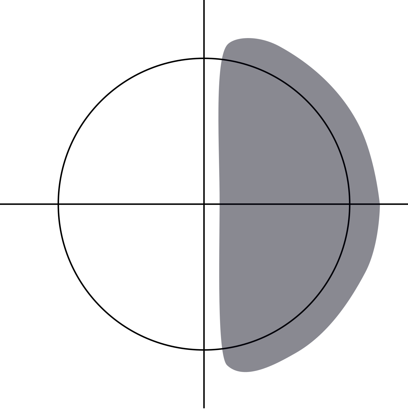
(c) t=$T_{5}^{\alpha}$

(d) t=$T_{6}^{\alpha}$

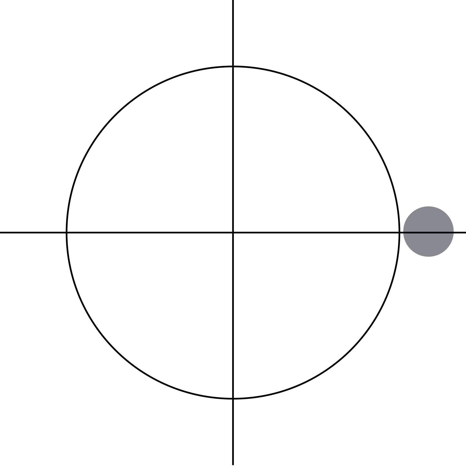
(e) t=$T_{7}^{\alpha}$

Figure 2: Outline of the semi-flow $F(g^{\alpha})$ in $\mathbb{R}^{2}$ at time $t$

Step 1: Since (1) is strongly contracting, we can choose $T_{1}^{\alpha}$ such that $\left|F(g^{\alpha})(T_{1}^{\alpha},x)\right|\leq 1+\alpha$ for all $x\in\mathbb{R}^{d}$.
Define $Y(t,y):=F(g^{\alpha}(t+T_{1}^{\alpha}))(t,y)$ for $y\in\mathbb{R}^{d}$ and write $t_{k}^{\alpha}:=T_{k}^{\alpha}-T_{1}^{\alpha}$ for $k=2,\dots,7$. Observe that it is sufficient to restrict the analysis to $Y(t,y)$ on the set $\bar{B}_{1+\alpha}$ since $Y(t,y)$ describes the dynamics of $F(g^{\alpha})$ after time $T_{1}^{\alpha}$. Denote by $\Pi_{k}$ the projection on the $k$-th component in $\mathbb{R}^{d}$.
In the steps 2 to 4, we concentrate on the movement of the point $y_{1}:=(-1-\alpha,0,\dots,0)\in\mathbb{R}^{d}$, choose $t_{2}^{\alpha},t_{3}^{\alpha}$ and $t_{4}^{\alpha}$ and show that $\Pi_{1}(Y(t_{4}^{\alpha},y_{1})>0$. This behavior we extend to the set $\bar{B}_{1+\alpha}$ in step 5 by choosing $\beta^{\alpha}$ and $t_{5}^{\alpha}$ suitable and showing that $\Pi_{1}(Y(t_{5}^{\alpha},y))>0$ for all $y\in\bar{B}_{1+\alpha}$. Observe that $\Pi_{1}(Y(s,y))>0$ implies that $\Pi_{1}(Y(t,y))>0$ for all $y\in\mathbb{R}^{d}$ and $0<s<t$ and define $t_{y}:=\inf\left\{t\geq 0:\Pi_{1}(Y(t,y))>0\right\}$ for $y\in\mathbb{R}^{d}$. Hence, $\Pi_{1}(Y(t,y))>0$ for all $t\geq t_{y}$. In the steps 6 and 7, we choose $t_{6}^{\alpha}$ and $t_{7}^{\alpha}$ and show the contraction.
Step 2: Set $y_{1}:=(-1-\alpha,0,\dots,0)\in\mathbb{R}^{d}$. Observe that $\Pi_{1}(F(t\mapsto 3\alpha t)(2,y_{1}))\geq-c_{1}^{\alpha}$. Choose $t_{2}^{\alpha}=2$.
Step 3: The function $\varphi$ as defined above describes the movement of $Y(\cdot+t_{2}^{\alpha},y_{2})$ started in $y_{2}:=(-c_{1}^{\alpha},0,\dots,0)\in\mathbb{R}^{d}$. Choose $t_{3}^{\alpha}$ such that $\varphi(t_{3}^{\alpha}-t_{2}^{\alpha})\geq-\alpha$. Then, $\Pi_{1}(Y(t_{3}^{\alpha},y_{2}))\geq-\alpha$.
Step 4: Let $y_{3}:=(-\alpha,0,\dots,0)\in\mathbb{R}^{d}$. Observe that $\Pi_{1}(F(t\mapsto(-2u^{\prime}(0)+1)\alpha t)(2,y_{3}))\geq\alpha$. Choose $t_{4}^{\alpha}=t_{3}^{\alpha}+2$. Then, $\Pi_{1}(Y(t_{4}^{\alpha},y_{1}))\geq\alpha>0$.
Step 5: Since $y\mapsto Y(t_{4}^{\alpha},y)$ is continuous, there exists a neighborhood of $y_{1}$ such that $\Pi_{1}(Y(t_{4}^{\alpha},y))>0$ for all $y$ in this neighborhood. Hence, there exists an $\eta^{\alpha}>0$ such that $\Pi_{1}(Y(t_{4}^{\alpha},y))<0$ for some $y\in S_{1+\alpha}$ implies that $\Pi(y)\geq-1-\alpha+\eta^{\alpha}$. Observe that

$$d\;\frac{\Pi_{1}(F(g^{\alpha})(t,y))}{\sqrt{\sum_{k=2}^{d}(\Pi_{k}(F(g^{\alpha})(t,y)))^{2}}}=\frac{1}{\sqrt{\sum_{k=2}^{d}(\Pi_{k}(F(g^{\alpha})(t,y)))^{2}}}\;dg^{\alpha}(t)$$

for all $y\in\mathbb{R}^{d}$. Observe that $|Y(t,y)|\leq 2$ for all $y\in\bar{B}_{1+\alpha}$ and $t_{4}^{\alpha}\leq t<t_{y}$. Hence,

$$\frac{\Pi_{1}(Y(t,y))}{\sqrt{\sum_{k=2}^{d}(\Pi_{k}(Y(t,y)))^{2}}}\geq-\frac{2}{\eta^{\alpha}}+\frac{1}{2}\beta^{\alpha}(t-t_{4}^{\alpha})$$

for all $y\in S_{1+\alpha}$ and $t_{4}^{\alpha}\leq t<t_{y}$. Set $\beta^{\alpha}:=\alpha\eta^{\alpha}$ and $t_{5}^{\alpha}:=t_{4}^{\alpha}+8\alpha^{-1}(\eta^{\alpha})^{-2}$. Then, $\Pi_{1}(Y(t_{5}^{\alpha},y))>0$ for any $y\in S_{1+\alpha}$. Moreover,

$$\hat{I}_{T_{5}^{\alpha}-T_{4}^{\alpha}}(g^{\alpha}(\cdot+T_{4}^{\alpha}))=(h^{\alpha}(T_{5}^{\alpha}))^{2}\left(T_{5}^{\alpha}-T_{4}^{\alpha}\right)=(\beta^{\alpha})^{2}\left(t_{5}^{\alpha}-t_{4}^{\alpha}\right)=8\alpha.$$

Step 6: Since $\Pi_{1}(Y(t_{5}^{\alpha},y))>0$ for any $y\in\bar{B}_{1+\alpha}$ and $\bar{B}_{1+\alpha}$ is closed, it follows that $\min_{y\in\bar{B}_{1+\alpha}}\Pi_{1}(Y(t_{5}^{\alpha},y))>0$. Choose $t_{6}^{\alpha}>t_{5}^{\alpha}$ such that $c_{1}^{\alpha}\leq\left|Y(t_{6}^{\alpha},y)\right|\leq 2$ for all $y\in\bar{B}_{1+\alpha}$.
Step 7: Since $\Pi_{1}(Y(t_{6}^{\alpha},x))>0$, $\left|Y(t_{6}^{\alpha},x)\right|\geq c_{1}^{\alpha}$ and $\Pi_{1}(g^{\alpha}(t))\geq 0$ for all $x\in\bar{B}_{1+\alpha}$ and $t\geq 0$, it holds that $\left|Y(t,x)\right|\geq c_{1}^{\alpha}$ for all $x\in\bar{B}_{1+\alpha}$ and $t_{6}^{\alpha}\leq t\leq t_{7}^{\alpha}$. Observe that $z:=(c_{2}^{\alpha},0,\dots,0)\in\mathbb{R}^{d}$ is a fixed point of $Y(t+t_{6}^{\alpha},\cdot)$. By convexity of $u$, for any $x=(x_{1},x_{2},\dots,x_{d})\in\mathbb{R}^{d}$ with $x_{1}>0$ and $|x|\geq c_{1}^{\alpha}$

$$d\,\left|Y(t+t_{6}^{\alpha},x)-z\right|^{2} \leq-\frac{1}{2}\left|Y(t+t_{6}^{\alpha},x)-z\right|^{2}\,\left(u^{\prime}(|Y(t+t_{6}^{\alpha},x)|^{2})+u^{\prime}(|z|^{2}))\right)\;dt$$

$$\leq-\frac{\alpha}{2}\left|Y(t+t_{6}^{\alpha},x)-z\right|^{2}\;dt.$$

By Gronwall’s inequality, it follows that

$$\left|Y(t+t_{6}^{\alpha},x)-z\right|\leq 4\,\exp\left(-\frac{\alpha t}{4}\right).$$

Choose $t_{7}^{\alpha}=t_{6}^{\alpha}+\frac{4}{\alpha}(\log 8-\log\delta)$. Combining all steps, it follows that $\left|F(g^{\alpha})(T_{7}^{\alpha},x)-F(g^{\alpha})(T_{7}^{\alpha},y)\right|\leq\delta$ for all $x,y\in\mathbb{R}^{d}$. ∎

Proposition 3.6.

Assume that the SDE (1) is strongly contracting. Set $V:=V(0,1,\infty)$. Then, for any $\delta>0$ and $\beta>0$ it holds that

$$\lim_{\varepsilon\rightarrow 0}\mathbb{P}\left(\tau_{3,\delta}^{\varepsilon}<\exp((V+\beta)/\varepsilon)\right)=1$$

and

$$\lim_{\varepsilon\rightarrow 0}\varepsilon\log\mathbb{E}\tau_{3,\delta}^{\varepsilon}\leq V.$$

Proof.

Let $0<\eta<\beta/2$. By Lemma 3.5 there exists $\varepsilon_{0}>0$ and $T>0$ such that

$$\mathbb{P}\left(\tau_{3,\delta}\leq T\right)\geq\exp((-V-\eta)/\varepsilon).$$

for all $\varepsilon\leq\varepsilon_{0}$. Conditioning on the event $\left\{\tau_{3,\delta}^{\varepsilon}>(k-1)T\right\}$ for $k=2,3,...$ yields

$$\mathbb{P}\left(\tau_{3,\delta}^{\varepsilon}>kT\right) =\mathbb{P}\left(\tau_{3,\delta}^{\varepsilon}>kT|\tau_{3,\delta}^{\varepsilon}>(k-1)T\right)\mathbb{P}\left(\tau_{3,\delta}^{\varepsilon}>(k-1)T\right)$$

$$\leq\mathbb{P}\left(\tau_{3,\delta}^{\varepsilon}>T\right)\mathbb{P}\left(\tau_{3,\delta}^{\varepsilon}>(k-1)T\right)$$

$$\leq\mathbb{P}\left(\tau_{3,\delta}^{\varepsilon}>T\right)^{k}$$

Therefore,

$$\mathbb{E}\tau_{3,\delta}^{\varepsilon} \leq T\left(1+\sum_{k=1}^{\infty}\mathbb{P}\left(\tau_{3,\delta}^{\varepsilon}>kT\right)\right)\leq T\left(1+\sum_{k=1}^{\infty}\left(1-\exp((-V-\eta)/\varepsilon)\right)^{k}\right)$$

$$\leq T\exp((V+\eta)/\varepsilon)$$

for all $\varepsilon\leq\varepsilon_{0}$. Using Markov’s inequality it follows that

$$\mathbb{P}\left(\tau_{3,\delta}^{\varepsilon}\geq\exp((V+\beta)/\varepsilon)\right)\leq T\exp(-\beta/(2\varepsilon))$$

for all $\varepsilon\leq\varepsilon_{0}$. ∎

Remark 3.7.

Observe that the upper bound for $\tau_{3,\delta}^{\varepsilon}$ as in Proposition 3.6 even hold for some RDS that do not synchronize.
In [8], an example of a SDE is presented which does not synchronize for small noise. The drift of this SDE is of the same form as in the SDE (1) while the noise merely acts in the first component. Hence, the arguments in Lemma 3.5 and Proposition 3.6 extend to this SDE since $g^{\alpha}$ in Lemma 3.5 is chosen to be $0$ in all components except for the first one.

3.4 Approaching the set attractor

Combining the estimates from the previous subsections, we get lower and upper bounds for these stopping times. These bounds show that the time a set requires to approach the attractor is roughly $\exp(V(0,1,\infty)/\varepsilon)$.

Theorem 3.8.

Assume that the SDE (1) is strongly contracting. Set $V:=V(0,1,\infty)$ and let $S_{1}\subset M\subset\mathbb{R}^{d}$. For any $\beta>0$ there exists $\delta_{0}>0$ such that for all $0<\delta\leq\delta_{0}$ it holds that

$$\lim_{\varepsilon\rightarrow 0}\mathbb{P}\left(\exp((V-\beta)/\varepsilon)<\tau_{1,2\delta}^{\varepsilon}\leq\tau_{2,\delta,M}^{\varepsilon}\leq\tau_{3,\delta}^{\varepsilon}<\exp((V+\beta)/\varepsilon)\right)=1$$

and

$$\lim_{\varepsilon\rightarrow 0}\varepsilon\log\mathbb{E}\tau^{\varepsilon}_{1,2\delta}=\lim_{\varepsilon\rightarrow 0}\varepsilon\log\mathbb{E}\tau_{2,\delta,M}^{\varepsilon}=\lim_{\varepsilon\rightarrow 0}\varepsilon\log\mathbb{E}\tau^{\varepsilon}_{3,\delta}=V.$$

Proof.

Using $\tau_{1,2\delta}^{\varepsilon}\leq\tau_{2,\delta,M}^{\varepsilon}\leq\tau_{3,\delta}^{\varepsilon}$, the statement follows by Corollary 3.4 and Proposition 3.6. ∎

4 Time required for a point to approach the attractor

4.1 Convergence to a process on the unit sphere

In this section, we show that the time required for a point to approach the attractor under the dynamics of (1) in dimension $d=2$ is exactly of order $\varepsilon^{-1}$. In particular, we give an estimate on the rate of convergence of a point under the dynamics of (1) towards the attractor.
Here, we consider the minimal weak point attractor $A^{X,\varepsilon}_{point}$. A minimal weak point attractor is a weak point attractor that is contained in any other weak point attractor. By [6, Theorem 3.1] and [4, Theorem 23] such a minimal weak point attractor exists.
In dimension $d=1$, the time until two points approach each other is the same as the time until the diameter of the of the interval between both points to get small. Hence, in dimension $d=1$ the time until a point to approach the attractor can be described by methods of section 3 and grows exponentially in $\varepsilon^{-1}$.
We concentrate on the case of dimension $d=2$ where the process behaves similar to a process on a unit sphere which is known to synchronize weakly. It remains as an open problem whether one can use similar arguments in higher dimensions as well.
We perform a time change and compare the accelerated process to a process on the unit sphere. Therefore, we write the accelerated process in polar coordinates. Precisely, we consider

$$\left(R_{t}^{\varepsilon}\cos\phi_{t}^{\varepsilon},R_{t}^{\varepsilon}\sin\phi_{t}^{\varepsilon}\right)=X_{t/\varepsilon}^{\varepsilon}.$$

Then,

$$d(R_{t}^{\varepsilon})^{2}=-\frac{4}{\varepsilon}(R_{t}^{\varepsilon})^{2}u^{\prime}((R_{t}^{\varepsilon})^{2})dt+2R_{t}^{\varepsilon}\cos\phi_{t}^{\varepsilon}d\tilde{W}_{t}^{1}+2R_{t}^{\varepsilon}\sin\phi_{t}^{\varepsilon}d\tilde{W}_{t}^{2}+2dt.$$ (9)

where $u^{\prime}$ is the first derivative of $u$ and

$$d\phi_{t}^{\varepsilon}=\frac{1}{R_{t}^{\varepsilon}}\left(-\sin\phi_{t}^{\varepsilon}d\tilde{W}_{t}^{1}+\cos\phi_{t}^{\varepsilon}d\tilde{W}_{t}^{2}\right)$$ (10)

where $\left(\tilde{W}_{t}^{1},\tilde{W}_{t}^{2}\right)=\sqrt{\varepsilon}W_{t/\varepsilon}$ and $(\tilde{W}^{1},\tilde{W}^{2})$ is a $2$-dimensional Brownian motion. As $\varepsilon\rightarrow 0$, the drift of $R_{t}^{\varepsilon}$ will move the radius close to $1$. Hence, we aim to compare $\phi_{t}^{\varepsilon}$ to the process

$$dZ_{t}=-\sin Z_{t}d\tilde{W}_{t}^{1}+\cos Z_{t}d\tilde{W}_{t}^{2}$$ (11)

on the limit cycle $S=\mathbb{R}/2\Pi\mathbb{Z}$. After we show that $R_{t}^{\varepsilon}$ is close to $1$ and $\phi_{t}^{\varepsilon}$ is close to $Z_{t}$, we will use that the RDS associated to (11) is known to synchronize weakly, i.e. every point in $S$ converges to a single random point.

Lemma 4.1.

Let $0<\alpha<\beta<1$, $T>0$ and $0<r_{1}<1<r_{2}<r_{3}<\infty$. Then, there exists an $\varepsilon_{0}>0$ such that

$$\mathbb{P}\left(r_{1}<R_{T}^{\varepsilon}<r_{2}\right)\geq 1-\beta$$

for all $\varepsilon\leq\varepsilon_{0}$ and any $\mathcal{F}^{-}$-measurable $X_{0}^{\varepsilon}$ satisfying

$$\mathbb{P}\left(R_{0}^{\varepsilon}\leq r_{3}\right)\geq 1-\alpha.$$

.

Proof.

Choose $k\in\mathbb{N}$ such that $2^{-k+1}\leq\beta-\alpha$ and set $t=\min\left\{1/2,T/(2k)\right\}$. Using (9),

$$\int_{0}^{t}R_{t}^{\varepsilon}\cos\phi_{t}^{\varepsilon}d\tilde{W}_{t}^{1}+\int_{0}^{t}R_{t}^{\varepsilon}\sin\phi_{t}^{\varepsilon}d\tilde{W}_{t}^{2}>0$$

implies that $(R_{s}^{\varepsilon})^{2}\geq 2t$ for some $s\leq t$. Set $r_{4}=\sqrt{2t}\leq 1$. Then

$$\mathbb{P}\left(R_{s}^{\varepsilon}\geq r_{4}\textrm{ for some }s\leq t\right)\geq 1/2.$$

Conditioning on the event $\left\{R_{s}^{\varepsilon}<r_{3}\textrm{ for all }s\leq(j-1)t\right\}$ for $j=2,3,...k$ yields to

$$\begin{split}\mathbb{P}\left(R_{s}^{\varepsilon}<r_{4}\textrm{ for all }s\leq T/2\right)&\leq\mathbb{P}\left(R_{s}^{\varepsilon}<r_{4}\textrm{ for all }s\leq kt\right)\\ &\leq 1/2\;\mathbb{P}\left(R_{s}^{\varepsilon}<r_{4}\textrm{ for all }s\leq(k-1)t\right)\\ &\leq 2^{-k}\leq(\beta-\alpha)/2.\end{split}$$ (12)

Combining this estimate and the assumption, it follows that

$$\mathbb{P}\left(r_{4}\leq R_{s}^{\varepsilon}\leq r_{3}\textrm{ for some }s\leq T/2\right)\geq 1-(\alpha+\beta)/2.$$

Let $r_{1}<r_{5}<1<r_{6}<r_{2}$. By Lemma 3.2, there exists $C,\varepsilon_{1}>0$ such that

$$\mathbb{P}\left(r_{5}<R_{s}^{\varepsilon}<r_{6}\textrm{ for some }s\leq T/2+\varepsilon C\right)\geq 1-(\alpha+2\beta)/3.$$

for all $\varepsilon\leq\varepsilon_{1}$. Hence, for all $\varepsilon\leq\min\left\{\varepsilon_{1},T/(2C)\right\}$

$$\mathbb{P}\left(r_{5}<R_{t}^{\varepsilon}<r_{6}\textrm{ for some }t\leq T\right)\geq 1-(\alpha+2\beta)/3..$$

Using Proposition 3.3, the statement follows. ∎

Lemma 4.2.

Let $0<\alpha<\beta<1$ and $\delta,T>0$. Then, there exists $\varepsilon_{0},\eta>0$ such that

$$\mathbb{P}\left(\max_{t\leq T}\left|R_{t}^{\varepsilon}-1\right|<\delta\textrm{ and }\max_{t\leq T}\left|\phi_{t}^{\varepsilon}-Z_{t}\right|<\delta\right)\geq 1-\beta$$

for all $\varepsilon\leq\varepsilon_{0}$ and all $\mathcal{F}^{-}$-measurable $X_{0}^{\varepsilon}$ and $Z_{0}$ satisfying

$$\mathbb{P}\left(\left|R_{0}^{\varepsilon}-1\right|<\eta\textrm{ and }\left|\phi_{0}^{\varepsilon}-Z_{0}\right|<\eta\right)\geq 1-\alpha.$$

Proof.

Choose $0<\eta<0.5\min\left\{\delta,1\right\}$ such that $\left(4\eta^{2}+128T\eta^{2}(1-2\eta)^{-2}\right)e^{16T}<(\beta-\alpha)\delta^{2}$. Define

$$B_{t}^{\varepsilon}:=\left\{\,\max_{s\leq t}\left|R_{s}^{\varepsilon}-1\right|<2\eta\right\}\cap\left\{\,\left|\varphi_{0}^{\varepsilon}-Z_{0}\right|<\eta\right\}.$$

for all $t\leq T$. Using Proposition 3.3 and the assumption, there exists $\varepsilon_{0}>0$ such that

$$\mathbb{P}\left(B_{T}^{\varepsilon}\right)\geq 1-(\alpha+\beta)/2$$

for all $\varepsilon\leq\varepsilon_{0}$. We use Doob’s inequality and Ito isometry to estimate

$$\mathbb{E}\max_{t\leq T}\left|\phi_{t}^{\varepsilon}-Z_{t}\right|^{2}\mathbbm{1}_{B_{T}^{\varepsilon}} \leq 2\mathbb{E}\left|\phi_{0}^{\varepsilon}-Z_{0}\right|^{2}\mathbbm{1}_{B_{T}^{\varepsilon}}+2\mathbb{E}\max_{t\leq T}\bigg{(}\int_{0}^{t}\left(\sin Z_{s}-\frac{1}{R_{s}^{\varepsilon}}\sin\phi_{s}^{\varepsilon}\right)\mathbbm{1}_{B_{s}^{\varepsilon}}\,dW_{s}^{1}$$

$$\qquad+\int_{0}^{t}\left(-\cos Z_{s}+\frac{1}{R_{s}^{\varepsilon}}\cos\phi_{s}^{\varepsilon}\right)\mathbbm{1}_{B_{s}^{\varepsilon}}\,dW_{s}^{2}\bigg{)}^{2}$$

$$\leq 2\eta^{2}+4\mathbb{E}\int_{0}^{T}\left(\left(\sin Z_{t}-\frac{1}{R_{t}^{\varepsilon}}\sin\phi_{t}^{\varepsilon}\right)^{2}+\left(-\cos Z_{t}+\frac{1}{R_{t}^{\varepsilon}}\cos\phi_{t}^{\varepsilon}\right)^{2}\right)\mathbbm{1}_{B_{t}^{\varepsilon}}\,dt$$

$$\leq 2\eta^{2}+16\,\mathbb{E}\int_{0}^{T}\left(\left|Z_{t}-\phi_{t}^{\varepsilon}\right|^{2}+\left|1-\frac{1}{R_{t}^{\varepsilon}}\right|^{2}\right)\mathbbm{1}_{B_{t}^{\varepsilon}}\,dt$$

$$\leq 2\eta^{2}+64T\frac{\eta^{2}}{(1-2\eta)^{2}}+16\int_{0}^{T}\mathbb{E}\max_{s\leq t}\left|Z_{s}-\phi_{s}^{\varepsilon}\right|^{2}\mathbbm{1}_{B_{t}^{\varepsilon}}\,dt.$$

Using Gronwall’s inequality, it follows that

$$\mathbb{E}\max_{t\leq T}\left|\phi_{t}^{\varepsilon}-Z_{t}\right|^{2}\mathbbm{1}_{B_{T}^{\varepsilon}}\leq\left(2\eta^{2}+64T\frac{\eta^{2}}{(1-2\eta)^{2}}\right)\,e^{16T}<(\beta-\alpha)\delta^{2}/2.$$

Using Markov inequality, we get

$$\mathbb{P}\left(\max_{t\leq T}\left|R_{t}^{\varepsilon}-1\right|<\delta\textrm{ and }\max_{t\leq T}\left|\phi_{t}^{\varepsilon}-Z_{t}\right|<\delta\right) \geq\mathbb{P}\left(B_{T}^{\varepsilon}\right)-\mathbb{P}\left(B_{T}^{\varepsilon}\textrm{ and }\max_{t\leq T}\left|\phi_{t}^{\varepsilon}-Z_{t}\right|\geq\delta\right)$$

$$\geq 1-(\alpha+\beta)/2-\delta^{-2}\,\mathbb{E}\max_{t\leq T}\left|\phi_{t}^{\varepsilon}-Z_{t}\right|^{2}\mathbbm{1}_{B_{T}^{\varepsilon}}$$

$$\geq 1-\alpha$$

for all $\varepsilon\leq\varepsilon_{0}$. ∎

4.2 Asymptotic stability of the process on the unit sphere

The SDE (11) has a stable point whose Lyapunov exponent is negative, see [2]. This random point is the minimal weak point attractor of the RDS associated to (11) which we in the following denote by $A^{Z}$. Observe that due to the time change the minimal weak point attractor $A^{Z}$ of the RDS associated to (11) at time $t$ is $A^{Z}(\theta_{t/\varepsilon}\omega)$. When we consider the distance of $A^{Z}$ to a point in $\mathbb{R}^{2}$, we identify with $A^{Z}$ the point $\left(\cos A^{Z},\sin A^{Z}\right)$ on the unit sphere.
Denote by $Z_{t}(Z_{0})$ the solution of (11) started in $Z_{0}$. We now show the rate of convergence of $Z_{t}(Z_{0})$ to $A^{Z}$, first for deterministic $Z_{0}$ and then for $\mathcal{F}^{-}$-measurable $Z_{0}$.

Lemma 4.3.

For any $\alpha>0$ and $0<\mu<1/2$ there exists $C>0$ such that

$$\mathbb{P}\left(\left|Z_{t}(Z_{0})-A^{Z}(\theta_{t/\varepsilon}\cdot)\right|\leq C\,e^{-\mu t}\textrm{ for all }t\geq 0\right)\geq 1-\alpha$$

for all $Z_{0}\in[0,2\Pi)$.

Proof.

By [2], the top Lyapunov exponent of (11) is $-1/2$. Stable manifold theorem implies that for all $0<\mu<0.5$ there exist a measurable $c(\omega)>0$ and a measurable neighborhood $U(\omega)$ of $A^{Z}(\omega)$ such that

$$\left|Z_{t}(x)-A^{Z}(\theta_{t/\varepsilon}\omega)\right|<c(\omega)e^{-\mu t}$$

for all $x\in U(\omega)$ and $t\geq 0$. Hence, for any $\alpha>0$ there exists some $\tilde{c},\delta>0$ such that

$$\mathbb{P}\left(\left|Z_{t}(x)-A^{Z}(\theta_{t/\varepsilon}\omega)\right|<\tilde{c}e^{-\mu t}\textrm{ for all }x\in A^{Z}(\omega)^{\delta}\textrm{ and }t\geq 0\right)\geq 1-\alpha/2.$$

Since $A^{Z}(\omega)$ is the attractor of the RDS associated to (11), there exists a time $T>0$ such that

$$\mathbb{P}\left(\left|Z_{T}(x)-A^{Z}(\theta_{T/\varepsilon}\omega)\right|<\delta\right)\geq 1-\alpha/2$$

for all $x\in[0,2\Pi)$. Combining these two estimates yields to

$$\mathbb{P}\left(\left|Z_{t}(x)-A^{Z}(\theta_{t/\varepsilon}\omega)\right|<\tilde{c}e^{-\mu(t-T)}\textrm{ for all }t\geq T\right)\geq 1-\alpha$$

for all $x\in[0,2\Pi)$ and $t\geq 0$. ∎

Proposition 4.4.

For any $\alpha>0$ and $0<\mu<0.5$ there exists $C>0$ such that

$$\mathbb{P}\left(\left|Z_{t}-A^{Z}(\theta_{t/\varepsilon}\cdot)\right|\leq C\,e^{-\mu t}\textrm{ for all }t\geq 0\right)\geq 1-\alpha$$

for all $\mathcal{F^{-}}$-measurable $Z_{0}$.

Proof.

The weak point attractor $A^{Z}(\omega)$ is an $\mathcal{F^{-}}$-measurable stable point. Reverting the time, one receives an $\mathcal{F^{+}}$-measurable unstable point $U^{Z}(\omega)$. Hence, $U^{Z}(\omega)$ and $A^{Z}(\omega)$ are independent. Under the dynamics of (11) every single deterministic point converges to the attractor. However, the unstable point does not converge to the attractor.
If the unstable point is in an interval and the attractor is not, then the time the endpoints of this interval require to approach the attractor is an upper bound for the time any point outside the interval requires to approach the attractor.
Let $n\in\mathbb{N}$ such that $\alpha n\geq 4$. We define

$$I_{k}:=\left[k\frac{2\Pi}{n},(k+1)\frac{2\Pi}{n}\right),\qquad P_{k}=k\frac{2\Pi}{n}\quad\textrm{ and }\quad P_{n}=P_{0}$$

for $0\leq k<n$. By Lemma 4.3 there exists $C>0$ such that

$$\mathbb{P}\left(\left|Z_{t}(P_{k})-A^{Z}(\theta_{t/\varepsilon}\cdot)\right|>C\,e^{-\mu t}\textrm{ for some }t\geq 0\right)\leq\frac{\alpha}{4n}$$

for all $0\leq k\leq n$. If $U^{Z}(\omega)\in I_{k}$ and $A(\omega)\not\in I_{k}$ for some $0\leq k<n$, then

$$\sup_{z\not\in I_{k}}\left|Z_{t}(z)-A^{Z}(\theta_{t/\varepsilon}\omega)\right|=\min\left\{\left|Z_{t}(P_{k})-A^{Z}(\theta_{t/\varepsilon}\omega)\right|,\left|Z_{t}(P_{k+1})-A^{Z}(\theta_{t/\varepsilon}\omega)\right|\right\}$$

for all $t\geq 0$. Therefore,

$$\mathbb{P}\left(\,\left|Z_{t}(Z_{0})-A^{Z}(\theta_{t/\varepsilon}\cdot)\right|\leq C\,e^{-\mu t}\textrm{ for all }t\geq 0\right)$$

$$\qquad\geq\sum_{k=0}^{n-1}\mathbb{P}\big{(}U^{Z}(\cdot)\in I_{k},A^{Z}(\cdot)\not\in I_{k},Z_{0}\not\in I_{k},\left|Z_{t}(P_{k})-A^{Z}(\theta_{t/\varepsilon}\cdot)\right|\leq C\,e^{-\mu t}$$

$$\qquad\qquad\quad\textrm{ and }\left|Z_{t}(P_{k+1})-A^{Z}(\theta_{t/\varepsilon}\cdot)\right|\leq C\,e^{-\mu t}\textrm{ for all }t\geq 0\big{)}$$

$$\qquad\geq\sum_{k=0}^{n-1}\big{(}\mathbb{P}\left(U^{Z}(\cdot)\in I_{k}\right)\mathbb{P}\left(A^{Z}(\cdot)\not\in I_{k},Z_{0}\not\in I_{k}\right)$$

$$\qquad\qquad\quad-\mathbb{P}\left(\left|Z_{t}(P_{k})-A^{Z}(\theta_{t/\varepsilon}\cdot)\right|>C\,e^{-\mu t}\textrm{ for some }t\geq 0\right)$$

$$\qquad\qquad\quad-\mathbb{P}\left(\left|Z_{t}(P_{k+1})-A^{Z}(\theta_{t/\varepsilon}\cdot)\right|>C\,e^{-\mu t}\textrm{ for some }t\geq 0\right)\big{)}$$

$$\qquad\geq\frac{1}{n}\sum_{k=0}^{n-1}\mathbb{P}\left(A^{Z}(\cdot)\not\in I_{k},Z_{0}\not\in I_{k}\right)-\alpha/2$$

$$\qquad\geq\frac{n-2}{n}-\alpha/2\geq 1-\alpha$$

for all $\mathcal{F^{-}}$-measurable $Z_{0}$. ∎

4.3 Approaching the point attractor

Combining the estimates from the previous subsections, we are able to show the rate of convergence of $X_{t/\varepsilon}^{\varepsilon}$ to $A^{Z}$. As a direct consequence, we get that $A^{Z}$ and $A^{X,\varepsilon}_{point}$ are close for small $\varepsilon$ and the upper bound for the rate of convergence of $X_{t/\varepsilon}^{\varepsilon}$ to $A^{X,\varepsilon}_{point}$. Moreover, we show that $X_{t}^{\varepsilon}$ does not approach its attractor on a faster time scale.

Proposition 4.5.

Let $0<\alpha<\beta<1$, $r>0$ and $0<\mu<0.5$. Then, there exists $C>0$ such that for all $T_{1},T_{3}>0$ there exists an $\varepsilon_{0}>0$ such that

$$\mathbb{P}\left(\left|X_{t/\varepsilon}^{\varepsilon}-A^{Z}(\theta_{t/\varepsilon}\cdot)\right|\leq Ce^{-\mu(t-T_{2})}\textrm{ for all }T_{2}\leq t\leq T_{2}+T_{3}\right)\geq 1-\beta$$

for all $0<\varepsilon\leq\varepsilon_{0}$, $T_{2}\geq T_{1}$ and all $\mathcal{F}^{-}$-measurable $X_{0}^{\varepsilon}$ satisfying

$$\mathbb{P}\left(R_{0}^{\varepsilon}\leq r\right)\geq 1-\alpha.$$

Proof.

Let $\varepsilon>0$. We start the SDE (11) in $Z_{T_{1}}^{\varepsilon}=\phi_{T_{1}}^{\varepsilon}$. By Proposition 4.4 there exists $c>0$ such that

$$\mathbb{P}\left(\left|Z_{t}-A^{Z}(\theta_{t/\varepsilon}\cdot)\right|\leq c\,e^{-\mu(t-T_{1})}\textrm{ for all }t\geq T_{1}\right)\geq 1-\alpha/2.$$

for all $\varepsilon>0$. Using Lemma 4.1 and 4.2, there exists $\varepsilon_{0}>0$ such that

$$\mathbb{P}\left(\max_{T_{1}\leq t\leq T_{1}+T_{3}}\left|R_{t}^{\varepsilon}-1\right|<e^{-\mu T_{3}}\textrm{ and }\max_{T_{1}\leq t\leq T_{1}+T_{3}}\left|\phi_{t}^{\varepsilon}-Z_{t}^{\varepsilon}\right|<e^{-\mu T_{3}}\right)\geq 1-\alpha/2$$

for all $\varepsilon\leq\varepsilon_{0}$. Setting $C:=c+2$ it follows that

$$\mathbb{P}\left(\left|X_{t/\varepsilon}^{\varepsilon}-A^{Z}(\theta_{t/\varepsilon}\cdot)\right|\leq Ce^{-\mu(t-T_{1})}\textrm{ for all }T_{1}\leq t\leq T_{1}+T_{3}\right)\geq 1-\alpha.$$

Using the same arguments for the process starting in $X_{(T_{2}-T_{1})/\varepsilon}^{\varepsilon}$ at time $(T_{2}-T_{1})/\varepsilon$, the statement follows. ∎

Remark 4.6.

Observe that the statement of Proposition 4.5 is not true if one takes the supremum over all $t\geq T$ inside the probability term. Precisely, for all $\delta,\varepsilon,T>0$

$$\mathbb{P}\left(\,\sup_{t\geq T}\,\left|X_{t/\varepsilon}^{\varepsilon}-A^{Z}(\theta_{t/\varepsilon}\cdot)\right|\leq\delta\right)=0$$

since the process $X_{t}^{\varepsilon}$ leaves a neighborhood of the unit sphere for some $t\geq T/\varepsilon$ almost surely.

Corollary 4.7.

For all $\alpha,\delta,T>0$ there exists an $\varepsilon_{0}>0$ such that

$$\mathbb{P}\left(\inf_{a\in A^{X,\varepsilon}_{point}(\theta_{t}\cdot)}|A^{Z}(\theta_{t}\cdot)-a|\leq\delta\textrm{ for all }0\leq t\leq T/\varepsilon\right)\geq 1-\alpha$$

for all $0<\varepsilon\leq\varepsilon_{0}$.

Proof.

By the construction of the minimal weak point attractor in [4, Theorem 23], the minimal weak point attractor of (1) has a $\mathcal{F}^{-}$-measurable version. We denote this version also by $A^{X,\varepsilon}_{point}$. Using [3, Theorem III.9], we can select an $\mathcal{F}^{-}$-measurable $x^{\varepsilon}(\omega)$ where

$$x^{\varepsilon}(\omega)\in\begin{cases}A^{X,\varepsilon}_{point}(\omega)\cap B_{2},&\textrm{if }A^{X,\varepsilon}_{point}(\omega)\cap B_{2}\not=\emptyset\\ \mathbb{R}^{2},&\textrm{else}.\end{cases}$$

Since the drift of (1) pushes any point outside the unit ball towards the unit ball, it holds that

$$\lim_{\varepsilon\rightarrow 0}\mathbb{P}\left(A^{X,\varepsilon}_{point}(\omega)\cap B_{2}=\emptyset\right)=0.$$

Applying Proposition 4.5, there exist some $\varepsilon_{1},s>0$ such that

$$\mathbb{P}\left(\left|X_{t/\varepsilon}^{\varepsilon}(x^{\varepsilon}(\cdot))-A^{Z}(\theta_{t/\varepsilon}\cdot)\right|\leq\delta\textrm{ for all }s\leq t\leq T\right)\geq 1-\alpha/2$$

for all $\varepsilon\leq\varepsilon_{1}$. Since $x^{\varepsilon}(\omega)\in A^{X,\varepsilon}_{point}(\omega)$ implies that $X_{t}^{\varepsilon}(x^{\varepsilon}(\omega))\in A^{X,\varepsilon}_{point}(\theta_{t}\omega)$, there exists $\varepsilon_{2}>0$ such that

$$\mathbb{P}\left(\inf_{a\in A^{X,\varepsilon}_{point}(\theta_{t}\cdot)}\left|A^{Z}(\theta_{t}\cdot)-a\right|\leq\delta\textrm{ for all }s/\varepsilon\leq t\leq(s+T)/\varepsilon\right)\geq 1-\alpha$$

for all $\varepsilon\leq\varepsilon_{2}$. Using $\theta_{s/\varepsilon}$-invariance of $\mathbb{P}$, the statement follows. ∎

Theorem 4.8.

Let $0<\alpha<\beta<1$, $r>0$ and $0<\mu<0.5$ Then, there exists $C>0$ such that for all $T_{1},T_{3}>0$ there exists an $\varepsilon_{0}>0$ such that

$$\mathbb{P}\left(\inf_{a\in A^{X,\varepsilon}_{point}(\theta_{t/\varepsilon}\cdot)}\left|X_{t/\varepsilon}^{\varepsilon}-a\right|\leq Ce^{-\mu(t-T_{2})}\textrm{ for all }T_{2}\leq t\leq T_{2}+T_{3}\right)\geq 1-\beta$$

for all $0<\varepsilon\leq\varepsilon_{0}$, $T_{2}\geq T_{1}$ and all $\mathcal{F}^{-}$-measurable $X_{0}^{\varepsilon}$ satisfying

$$\mathbb{P}\left(R_{0}^{\varepsilon}\leq r\right)\geq 1-\alpha.$$

Proof.

Apply Proposition 4.5 and Corollary 4.7 and use the triangle inequality. ∎

Theorem 4.9.

For any $\alpha>0$ there exist $\varepsilon_{0},\delta,T>0$ such that

$$\mathbb{P}\left(\sup_{a\in A^{X,\varepsilon}_{point}(\theta_{t}\cdot)}\left|X_{t}^{\varepsilon}-a\right|>\delta\textrm{ for all }0\leq t\leq T/\varepsilon\right)\geq 1-\alpha$$

for all $\varepsilon\leq\varepsilon_{0}$ and all deterministic $X_{0}^{\varepsilon}\in\mathbb{R}^{2}$.

Proof.

Let $\gamma,T>0$ such that $20\gamma\leq\alpha\Pi$ and $10T\leq\alpha\gamma^{2}$. By Lemma 4.2 there exists $0<2\delta<\sin\gamma$ and $\varepsilon_{0}>0$ such that for all $0<\varepsilon\leq\varepsilon_{0}$

$$\mathbb{P}\left(\left|\phi_{t}^{\varepsilon}-Z^{\varepsilon}\right|\leq\gamma\textrm{ for all }\sigma^{\delta,\varepsilon}\leq t\leq T\right)\geq 1-\alpha/5$$

where $\sigma^{\delta,\varepsilon}:=\inf\left\{t\geq 0:\left|R_{t}^{\varepsilon}-1\right|\leq 2\delta\right\}$ and $Z^{\varepsilon}_{t}$ is the solution to (11) started in $Z^{\varepsilon}_{\sigma^{\delta,\varepsilon}}=\phi_{\sigma^{\delta,\varepsilon}}^{\varepsilon}$. Then,

$$\mathbb{P}\left(\left|X_{t/\varepsilon}-A^{Z}(\theta_{t/\varepsilon}\cdot)\right|>2\delta\textrm{ for all }t\leq T\right)$$

$$\qquad\geq\mathbb{P}\left(\left|X_{t/\varepsilon}-A^{Z}(\theta_{t/\varepsilon}\cdot)\right|>\sin\gamma\textrm{ for all }\sigma^{\delta,\varepsilon}\leq t\leq T\right)$$

$$\qquad\geq\mathbb{P}\left(\left|\phi_{t}^{\varepsilon}-A^{Z}(\theta_{t/\varepsilon}\cdot)\right|>\gamma\textrm{ for all }\sigma^{\delta,\varepsilon}\leq t\leq T\right)$$

$$\qquad\geq\mathbb{P}\left(\left|\phi_{t}^{\varepsilon}-Z^{\varepsilon}_{t}\right|\leq\gamma\textrm{ and }\left|Z^{\varepsilon}_{t}-A^{Z}(\theta_{t/\varepsilon}\cdot)\right|>2\gamma\textrm{ for all }\sigma^{\delta,\varepsilon}\leq t\leq T\right)$$

$$\qquad\geq\mathbb{P}\left(\left|Z^{\varepsilon}_{t}-A^{Z}(\theta_{t/\varepsilon}\cdot)\right|>2\gamma\textrm{ for all }\sigma^{\delta,\varepsilon}\leq t\leq T\right)-\alpha/5.$$

Independence of $Z^{\varepsilon}_{\sigma^{\delta,\varepsilon}}$ and $A^{Z}(\cdot)$ implies

$$\mathbb{P}\left(\left|Z^{\varepsilon}_{\sigma^{\delta,\varepsilon}}-A^{Z}(\cdot)\right|\leq 4\gamma\right)=\frac{8\gamma}{2\Pi}\leq\alpha/5.$$

Since $T$ was chosen small, it holds that

$$\mathbb{P}\left(\left|Z^{\varepsilon}_{t}-A^{Z}(\theta_{t/\varepsilon}\cdot)\right|>2\gamma\textrm{ for all }\sigma^{\delta,\varepsilon}\leq t\leq T\right)$$

$$\qquad\geq\mathbb{P}\left(\left|Z^{\varepsilon}_{\sigma^{\delta,\varepsilon}}-A^{Z}(\cdot)\right|>4\gamma,\left|Z^{\varepsilon}_{t}-Z^{\varepsilon}_{\sigma^{\delta,\varepsilon}}\right|\leq\gamma\textrm{ and }\left|A^{Z}(\cdot)-A^{Z}(\theta_{t/\varepsilon}\cdot)\right|\leq\gamma\textrm{ for all }\sigma^{\delta,\varepsilon}\leq t\leq T\right)$$

$$\qquad\geq 1-\alpha/5-\mathbb{P}\left(\max_{\sigma^{\delta,\varepsilon}\leq t\leq T}\left|Z^{\varepsilon}_{t}-Z^{\varepsilon}_{\sigma^{\delta,\varepsilon}}\right|>\gamma\right)-\mathbb{P}\left(\max_{\sigma^{\delta,\varepsilon}\leq t\leq T}\left|A^{Z}(\cdot)-A^{Z}(\theta_{t/\varepsilon}\cdot)\right|>\gamma\right)$$

$$\qquad\geq 1-3\alpha/5$$

Therefore,

$$\mathbb{P}\left(\left|X^{\varepsilon}_{t/\varepsilon}-A^{Z}(\theta_{t/\varepsilon}\cdot)\right|>2\delta\textrm{ for all }t\leq T\right)\geq 1-4\alpha/5.$$

Applying Corollary 4.7, the statement follows. ∎

For small $\delta>0$ denote by

$$\underline{\tau_{0,\delta,x}^{\varepsilon}}:=\inf\left\{t\geq 0:\inf_{a\in A^{X,\varepsilon}_{point}(\theta_{t}\cdot)}\left|X_{t}^{\varepsilon}(x)-a\right|\leq\delta\right\}$$

and

$$\overline{\tau_{0,\delta,x}^{\varepsilon}}:=\inf\left\{t\geq 0:\sup_{a\in A^{X,\varepsilon}_{point}(\theta_{t}\cdot)}\left|X_{t}^{\varepsilon}(x)-a\right|\leq\delta\right\}$$

the time the process $X_{t}^{\varepsilon}$ started in $x\in\mathbb{R}^{2}$ requires to approach some point respectively all points of the minimal weak point attractor $A^{X,\varepsilon}_{point}$. Observe that $\underline{\tau_{0,\delta,x}^{\varepsilon}}\leq\overline{\tau_{0,\delta,x}^{\varepsilon}}$. If the RDS associated to (1) synchronize both quantities coincide.

Corollary 4.10.

For any $\alpha>0$ there exists some $\delta_{0}>0$ such that for all $0<\delta\leq\delta_{0}$ there exist $\varepsilon_{0},T_{1},T_{2}>0$ such that

$$\mathbb{P}\left(\underline{\tau_{0,\delta,x}^{\varepsilon}}<T_{2}/\varepsilon\textrm{ and }\overline{\tau_{0,\delta,x}^{\varepsilon}}>T_{1}/\varepsilon\right)\geq 1-\alpha$$

for all $0<\varepsilon\leq\varepsilon_{0}$ and $x\in\mathbb{R}^{2}$. In particular, if the RDS associated to (1) synchronize weakly, then

$$\mathbb{P}\left(T_{1}/\varepsilon<\underline{\tau_{0,\delta,x}^{\varepsilon}}=\overline{\tau_{0,\delta,x}^{\varepsilon}}<T_{2}/\varepsilon\right)\geq 1-\alpha$$

Proof.

The lower bound follows by theorem 4.9 and the upper bound by theorem 4.8. ∎

Remark 4.11.

In contrast to Corollary 4.10, if $u$ has more than one local minima the time until a point approach the attractor under the dynamics of (1) can increase exponentially in $\varepsilon^{-1}$. For this purpose, observe that one can find a lower bound for the time until the paths of the solution started in different minima approach each other using the difference of the potential $U$ in the minima and similar arguments as in section 3.2.
Hence, in the case of $u$ having multiple minima, the difference between the time a point and a set requires to approach the attractor is not as significant as in the case where $u$ has exactly one minimum.

References

- [1] L. Arnold. Random Dynamical Systems. Springer Monographs in Mathematics. Springer-Verlag, Berlin, 1998.
- [2] P. H. Baxendale. Asymptotic behaviour of stochastic flows of diffeomorphisms. In Stochastic processes and their applications (Nagoya, 1985), volume 1203 of Lecture Notes in Math., pages 1–19. Springer, Berlin, 1986.
- [3] C. Castaing and M. Valadier. Convex Analysis and Measurable Multifunctions. Lecture Notes in Mathematics, Vol. 580. Springer-Verlag, Berlin-New York, 1977.
- [4] H. Crauel and M. Scheutzow. Minimal random attractors. J. Differential Equations, 265(2):702–718, 2018.
- [5] A. Dembo and O. Zeitouni. Large Deviations Techniques and Applications, volume 38 of Applications of Mathematics (New York). Springer-Verlag, New York, second edition, 1998.
- [6] G. Dimitroff and M. Scheutzow. Attractors and expansion for Brownian flows. Electron. J. Probab., 16:no. 42, 1193–1213, 2011.
- [7] F. Flandoli, B. Gess, and M. Scheutzow. Synchronization by noise. Probab. Theory Related Fields, 168(3-4):511–556, 2017.
- [8] I. Vorkastner. Noise dependent synchronization of a degenerate SDE. Stoch. Dyn., 18(1):1850007, 21, 2018.