The Core Mass Function Across Galactic Environments. II.
Infrared Dark Cloud Clumps

Abstract

We study the core mass function (CMF) within 32 dense clumps in seven infrared dark clouds (IRDCs) with the Atacama Large Millimeter/submillimeter Array (ALMA) via 1.3 mm continuum emission at a resolution of $\sim$1″. We have identified 107 cores with the dendrogram algorithm, with a median radius of about 0.02 pc. Their masses range from 0.261 to 178 $M_{\odot}$. After applying completeness corrections, we fit the combined IRDC CMF with a power law of the form $dN/d\>{\rm log}M\propto M^{-\alpha}$ and derive an index of $\alpha\simeq 0.86\pm 0.11$ for $M\geq 0.79\>M_{\odot}$ and $\alpha\simeq 0.70\pm 0.13$ for $M\geq 1.26\>M_{\odot}$, which is a significantly more top-heavy distribution than the Salpeter stellar initial mass function (IMF) index of 1.35. We also make a direct comparison of these IRDC clump CMF results to those measured in the more evolved protocluster G286 derived with similar methods, which have $\alpha\simeq 1.29\pm 0.19$ and $1.08\pm 0.27$ in these mass ranges, respectively. These results provide a hint that, especially for the $M\geq 1.26\>M_{\odot}$ range where completeness corrections are modest, the CMF in high pressure, early-stage environments of IRDC clumps may be top-heavy compared to that in the more evolved, global environment of the G286 protoclusters. However, larger samples of cores probing these different environments are needed to better establish the robustness of this potential CMF variation.

=1

1 Introduction

The origin of the stellar initial mass function (IMF) remains one of the most important unsolved problems in astrophysics. In general, the IMF can be described as having a broad peak just below $1\>M_{\odot}$, similar in shape to a log normal, but then extending with a power law form at high masses (see, e.g., Bastian et al. 2010), i.e.,

$$\frac{{\rm d}N}{{\rm d}{\rm log}M}\propto{M}^{-\alpha}.$$ (1)

Salpeter (1955) derived $\alpha\simeq 1.35$ between 0.4 and 10 $M_{\odot}$ and this value has remained valid as the standard description of the $\gtrsim 1\>M_{\odot}$ IMF from more recent studies.

Observations of dense cores show that the core mass function (CMF) may be similar in shape to the IMF (e.g., Alves et al. 2007; André et al. 2010; Offner et al. 2014; Könyves et al. 2015; Ohashi et al. 2016; Cheng et al. 2018). Such a similarity is taken as evidence that the stellar IMF is in large part determined by the fragmentation process in molecular clouds, after also allowing for a core to star formation efficiency. However, to most accurately test such a scenario, then observationally one should ideally measure the pre-stellar core (PSC) mass function, with PSCs being cores at an evolutionary stage just before the onset of star formation. This method has been carried out using FIR Herschel imaging of nearby regions, such as Aquila ($d=$260 pc), by, e.g., Könyves et al. (2015), who find a pre-stellar core mass function (PSCMF) that is similar in shape to the stellar IMF.

Unfortunately identifying PSCs in more distant star-forming regions is a non-trivial task. Using mm continuum emission to identify cores, i.e., the thermal emission from dust, is the typical method adopted (and will be the one used in this paper). This then allows a measure of the mass of the sources, assuming given dust emissivities, dust-to-gas mass ratio and dust temperature. At this point the sample likely contains a mixture of prestellar cores and protostellar cores, and with the latter tending to be more easily detected given their internal heating. Attempts can then be made to remove obvious protostellar sources, e.g., those cores associated with infrared or x-ray emission or with outflow tracers. Such an approach was adopted by Ohashi et al. (2016), who first identified 48 cores in IRDC G14.225-0.506 from 3 mm continuum emission and then proposed 28 of these to be PSCs, based on a lack of IR or x-ray emission. However, in high column density regions such as IRDCs, lack of detected IR emission, e.g., from Spitzer MIPSGAL 24 $\rm\mu m$ images (Carey et al. 2009), is no guarantee a core is pre-stellar, as found by, e.g., Tan et al. (2016), who find that the presence of protostellar outflows, e.g., as traced by CO, can be a more powerful probe of protostellar activity depending on the extinction in the region. Furthermore, even if a core is identified as being pre-stellar from the above methods, it is not clear at which evolutionary stage it is at, i.e., whether it will grow much more in mass before forming a star.

An alternative approach is to try and select PSCs that are on the verge of forming stars via certain chemical species, especially deuterated species, such as $\rm N_{2}D^{+}$ (see, e.g., Caselli & Ceccarelli 2012; Tan et al. 2013; Kong et al. 2017). However, this requires very sensitive observations, and then the question of measuring the masses of the PSCs still needs to be addressed, e.g., via associated mm continuum emission or dynamically via line widths from some measured size scale.

Given the above challenges, a first step for distant regions is to characterize the combined pre-stellar and protostellar CMF, by simply treating all the detected sources as cores of interest. This approach has been adopted by, e.g., Beuther & Schilke (2004), Zhang et al. (2015), Cheng et al. (2018) and Motte et al. (2018). Such an approach, which is the one we will also adopt in this paper, is really a measurement of the mm luminosity function of “cores” with potentially a mixture of PSCs and protostellar cores being included in the sample, although, it is the latter, being warmer, that will tend to be identified in a given protocluster.

Since there are large potential systematic uncertainties associated with both core identification and core mass measurement, it is important to attempt to provide uniform and consistent observational metrics of core populations in different star-forming regions and environments to allow comparison of relative properties. With this goal in mind, we derive the mm-continuum-based CMF from observations of dense regions of Infrared Dark Clouds (IRDCs), thought to be representative of early stages of massive star and star cluster formation (see, e.g., Tan et al. 2014). Most importantly, we use the same methods as our previous study of the more evolved protocluster G286.21+0.17 (hereafter G286) (Cheng et al. 2018, hereafter Paper I).

There have been several previous studies of clump and core mass functions in IRDCs. Rathborne et al. (2006) measured an IRDC clump ($\sim$0.3 pc-scale) mass function, with high-end power law slope $\alpha\simeq 1.1\pm 0.4$ above a mass of $100\>M_{\odot}$ via 1.2 mm continuum emission. Ragan et al. (2009) identified structures on $\sim$0.1pc scales and found $\alpha\simeq 0.76\pm 0.05$ from 30 to 3000 $M_{\odot}$ through dust extinction. Zhang et al. (2015) measured the masses of 38 dense cores (with $\sim$0.01 pc scales) in the massive IRDC G28.34+0.06, clump P1 (also known as C2 in the sample of Butler & Tan 2009, 2012) via 1.3 mm continuum emission and found a lack of cores in the range 1 to 2 $M_{\odot}$ compared with that expected from an extrapolation of the observed higher-mass population with a Salpeter power law mass function. Finally, as mentioned above, Ohashi et al. (2016) studied IRDC G14.225-0.506 and identified 28 starless cores on scales $\sim$0.03 pc and derived $\alpha\simeq 1.6\pm 0.7$ from with masses ranging from 2.4 to 14 $M_{\odot}$ via 3 mm dust continuum emission.

We have conducted a 1.3 mm continuum and line survey of 32 IRDC clumps with ALMA in Cycle 2. These regions are of high mass surface density, being selected from mid-infrared (Spitzer-IRAC 8 $\mu$m) extinction (MIREX) maps of 10 IRDCs (A-J) (Butler & Tan 2012). The distances to the sources, based on near kinematic distance estimates, range from 2.4 kpc to 5.7 kpc. The first goal of this survey was to identify PSCs via $\rm N_{2}D^{+}(3-2)$ emission, with about 100 such core candidates detected (Kong et al. 2017). Here we report on the analysis of the 1.3 mm continuum cores and derivation of the CMF in these 32 IRDC clumps. In §2 we describe the observations and analysis methods. In §3 we present our results on the construction of the CMF, including with completeness corrections, and the comparison to G286. We discuss the implications of our results and conclude in §4.

2 Observations and Analysis Methods

2.1 Observational Data

We use data from ALMA Cycle 2 project 2013.1.00806.S (PI: Tan), which observed 32 IRDC clumps on 04-Jan-2015, 10-Apr-2015 and 23-Apr-2015, using 29 12 m antennas in the array. The total observation time including calibration is 2.4 hr. The actual on-source time is $\sim$2-3 min for each pointing (30 pointings in total).

The spectral set-up included a continuum band centered at 231.55 GHz (LSRK frame) with width 1.875 GHz from 230.615 GHz to 232.490 GHz. At 1.3 mm, the primary beam of the ALMA 12 m antennas is $27\arcsec$ (FWHM) and the largest recoverable scale for the array is $\sim 11\arcsec$ ($\sim$ 0.3 pc at a typical distance of 5 kpc). No ACA observations were performed. The sample of 32 targets was divided into two tracks, each containing 15 pointings. Track 1, with reference velocity of +58 $\rm kms^{-1}$, includes A1, A2, A3, B1, B2, C2, C3, C4, C5, C6, C7, C8, C9, E1, E2 (following the nomenclature of Butler & Tan 2012). Track 2, with reference velocity of +66 $\rm kms^{-1}$, includes D1, D2 (also contains D4), D3, D5 (also contains D7), D6, D8, D9, F3, F4, H1, H2, H3, H4, H5, H6. The continuum image reaches a 1$\sigma$ rms noise of $\sim$0.2 mJy in a synthesized beam of $\sim$ 1.36$\arcsec$ $\times$ 0.82$\arcsec$. Other basebands were tuned to observe N₂D⁺(3-2), SiO(5-4), $\rm C^{18}O$(2-1), DCN(3-2), DCO⁺(3-2) and $\rm CH_{3}OH\ (5(1,4)-4(2,2))$. These data have mostly been presented by Kong et al. (2017), with the SiO(5-4) data to be presented by Liu et al. (in prep.).

To investigate the flux recovery of our 12m data, we use the archival data from the Bolocam Galactic Plane Survey (BGPS) (Aguirre et al. 2011; Ginsburg et al. 2013), which are the closest in frequency single-dish millimeter data available. We measure the flux density in both ALMA and BGPS images of each clump (the aperture is 27$\arcsec$ across, i.e., one ALMA primary beam size) and then convert the BGPS flux density measurements at 267.8 GHz to the mean ALMA frequency of 231.6 GHz via $S_{\nu}\propto\nu^{\alpha_{\nu}}$ assuming $\alpha_{\nu}=3.5\pm 0.5$. For the ALMA data we measure the total flux above a 3$\sigma$ noise level threshold. Finally we derive a median flux recovery fraction of 0.19 $\pm$ 0.02. As expected, these 12m array only ALMA observations filter out most of the total continuum flux from the clumps.

2.2 Core Identification

Our main objective is to identify cores using standard, reproducable methods. In particular, we aim to follow the methods used in our Paper I study of the G286 protocluster as closely as possible so that a direct comparison of the CMFs can be made. Thus for our fiducial core finding algorithm we will adopt the dendrogram (Rosolowsky et al. 2008) method as implemented in the astrodendro python package. We set the minimum threshold intensity required to identify a parent tree structure (trunk) to be $4\sigma$, where $\sigma$ is the rms noise level in the continuum image prior to primary beam correction, with typical value $\sigma\sim 0.2\>{\rm mJy\ beam}^{-1}$, except for C9 where $\sigma=0.6\>{\rm mJy\ beam}^{-1}$ due to its large dynamic range.

For identification of nested substructures (branches and leaves), we require an additional $1\sigma$ increase in intensity. Finally, we set a minimum area of half the synthesized beam size for a leaf structure to be identified. These “leaves” are the identified “cores”. The parameters associated with these three choices are the same as the fiducial choices of Paper I. We note that Paper I carried out an extensive exploration of the effects of these parameter choices on the derived CMF, which we do not carry out here, rather focusing on the comparison of fiducial-method CMFs between the IRDC clump and G286 protocluster environments.

While the dendrogram algorithm is our preferred fiducial method of core identification, following Paper I, we will also consider the effects of using the clumpfind algorithm (Williams et al. 1994). The main differences of clumpfind are that it is non-hierarchical, so that all the detected signal is apportioned between the “cores”, leading, in general, to more massive cores and thus a more top-heavy CMF (see Paper I).

We note that one difference between our methodology compared to that of Paper I is that our core identification is done in images before primary beam correction. This is because our observational data set consists of multiple individual pointings, whereas that of Paper I is a mosaic of a single region, i.e., with a more uniform noise level. The result of this difference is that our threshold levels that define cores vary depending on position in the image. Our method of implementing completeness corrections, described below, attempts to correct for this effect. Note, we restrict core identification to the area within the FWHM primary beam in each image.

2.3 Core Mass Estimation

We estimate core masses by assuming optically thin thermal emission from dust, following the same assumptions adopted in Paper I. The total mass surface density corresponding to a given specific intensity of mm continuum emission is

$$\Sigma_{\rm mm} = 0.369\frac{F_{\nu}}{\rm mJy}\frac{(1\arcsec)^{2}}{\Omega}\frac{\lambda_{1.3}^{3}}{\kappa_{\nu,0.00638}}$$

$$\times\left[{\rm exp}\left(0.553T_{d,20}^{-1}\lambda_{1.3}^{-1}\right)-1\right]\>{\rm g\>cm^{-2}}$$

$$\rightarrow 0.272\frac{F_{\nu}}{\rm mJy}\frac{(1\arcsec)^{2}}{\Omega}\>{\rm g\>cm^{-2}},$$

where $F_{\nu}$ is the total integrated flux over solid angle $\Omega$, $\kappa_{\nu,0.00638}\equiv\kappa_{\nu}/({\rm 6.38\times 10^{-3}\>cm^{2}\>g}^{-1})$ is the dust absorption coefficient, $\lambda_{1.3}=\lambda/1.30\>{\rm mm}$ and $T_{d,20}=T_{d}/20\>{\rm K}$ with $T_{d}$ being the dust temperature. To obtain the above fiducial normalization of $\kappa_{\nu}$, we assume an opacity per unit dust mass $\kappa_{\rm 1.3mm,d}=0.899\>{\rm cm^{2}g}^{-1}$ (moderately coagulated thin ice mantle model of Ossenkopf & Henning 1994), which then gives $\kappa_{\rm 1.3mm}={\rm 6.38\times 10^{-3}\>cm^{2}\>g}^{-1}$ using a gas-to-refractory-component-dust ratio of 141 (Draine 2011). The numerical factor following the $\rightarrow$ in the final line shows the fiducial case where $\lambda_{1.3}=1$ and $T_{d,20}=1$.

We note that even though temperatures in IRDCs are often measured to be cooler than $20\>K$, e.g., $\sim 15\>$K from studies using inversion transitions of $\rm NH_{3}$ (e.g., Pillai et al. 2006; Sokolov et al. 2017) or from multiwavelength sub-mm continuum emission maps (e.g., Lim et al. 2016), we expect that most of the cores identified in our images are protostellar cores that are internally heated to somewhat higher temperatures. If temperatures of 15 K or 30 K were to be adopted, then the mass estimates would differ by factors of 1.48 and 0.604, respectively.

2.4 Core Flux Recovery and Completeness Corrections

Following Paper I, we estimate two correction factors needed to estimate a “true” CMF from a “raw” observed CMF. The first factor is the flux recovery fraction, $f_{\rm flux}$; the second factor is the number recovery fraction, $f_{\rm num}$.

To evaluate these factors, artificial cores of a given mass (i.e., after primary beam correction) are inserted into each of the IRDC images, with three sources being inserted at a given time at random locations within the primary beam and this exercise repeated 50 times. This enables 150 experiments for each core mass. We note that the choice of random placement within the primary beam is different from that adopted in Paper I, which used the ACA-only image of the mosaic region as a weighting factor for core placement. We also note that our method means that cores of a given mass that are placed near the edge of the primary beam have smaller fluxes in the image and thus are harder to detect. We explore a range of masses from $10^{-1}$ to $10^{1.2}\>M_{\odot}$ with even spacing of 0.2 in log $M$. We assume the flux of the artificial cores has a gaussian distribution with the shape of the synthesized beam. This is an approximation that is most accurate in the limit of small, unresolved cores, which is where the correction factors become most important. The dendrogram algorithm is run to determine if the cores are recovered and then the recovered flux is compared to the true flux.

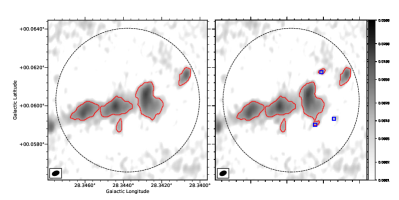
Figure 1: An example of artificial core insertion and recovery to evaluate completeness corrections for the C2 clump. (a) Left: Original 1.3 mm continuum image of the region (intensity scale in Jy beam^-1; dashed circle shows FWHM of primary beam; synthesized beam shown in bottom left), with boundaries of the identified cores shown in red. (b) Right: Same as (a) but now after inserting three artificial cores of $1.6\>M_{\odot}$ at random locations, with their centers marked by blue squares. Cores identified by the dendrogram algorithm are again marked with red contours: two out of three of the artificial cores are found.

An example of this procedure is shown in Figure 1. We can tell from the figure that whether a core of $\sim 1.6\>M_{\odot}$, which has a peak flux of $\sim 10\ \sigma$ at 5.0 kpc, can be detected depends on its location within the filed of view, i.e., being harder to detect near the edge of the primary beam, and also on the local background. The local background can have two main effects. First, if a faint core happens to be placed on an already identified stronger core, then the artificial core is likely to be undetected due to confusion. Second, if a faint core is placed on a region of emission in the original image that was too faint to be detected as a core, this increases the chances that the core will now be recovered by the core finding algorithm. In this case its recovered flux will have been artificially boosted by the presence of this background emission, though the total recovered flux may still be less than that inserted, e.g., due to the threshold criteria of core finding algorithm.

The median value of the ratio of recovered to true flux defines $f_{\rm flux}$, with this quantity being measured both as a function of true flux (mass) and of recovered flux (mass). The ratio of the actual number of cores recovered to the number inserted defines $f_{\rm num}$. The derived values of $f_{\rm flux}$ and $f_{\rm num}$ are presented below in §3.

3 Results

3.1 Continuum Images

The continuum images of the 30 positions in the IRDCs, covering 32 clumps, are shown in Figure 2, together with the identified cores (i.e., leaves from the dendrogram algorithm). The size of the FWHM of the primary beam is shown with a dashed circle in each image.

Overall we have identified 107 cores in these images. Note that we only identify cores that are within the primary beam. Although there may be true cores that show strong emission outside the primary beam, as in B2 and C2, in most cases the noise outside is relatively high and thus it is harder to identify cores of a given mass. We also note that we identify cores in all the regions apart from C3 and D2. Cores are named as, e.g., A1c1, A1c2, etc, in the region A1, with the numbering order from higher to lower Galactic latitude.

The properties of the identified cores (after primary beam correction) are listed in Table 1. The masses range from $0.261M_{\odot}$ to $178\>M_{\odot}$ (0.150 $M_{\odot}$ to 178 $M_{\odot}$ without flux correction), given our fiducial methods of mass estimation. The median radius of the cores is $R_{c}\sim 0.02$ pc, with the radii evaluated as $R_{c}=\sqrt{A/\pi}$, where $A$ is the projected area of the core. We then evaluate the mean mass surface density of the cores, $\Sigma_{c}\equiv M/A$, which have values $\gtrsim 0.3\>{\rm g\>cm}^{-2}$. This is consistent with expectations of the Turbulent Core Model of McKee & Tan (2003) given that the mass surface densities of the IRDC clump environments are at about this level of $\sim 0.3\>{\rm g\>cm}^{-2}$ (Butler & Tan 2012). We also evaluate the mean H nuclei number density in the cores, $n_{{\rm H},c}\equiv M_{c}/(\mu_{\rm H}V)$, where $\mu_{\rm H}=1.4m_{\rm H}$ is the mean mass per H assuming $n_{\rm He}=0.1n_{\rm H}$ and $V=4\pi R_{c}^{3}/3$. The mean value of ${\rm log}_{10}(n_{{\rm H},c}/{\rm cm}^{-3})$ is 6.58, with a dispersion of 0.34.

From an inspection of the molecular line data of these regions, as presented by Kong et al. (2017), we note that more than half of the cores are associated with molecular line emission, e.g., $\rm N_{2}D^{+}$(3-2), DCN(3-2), DCO⁺(3-2), C¹⁸O(2-1) and, occasionally, SiO(5-4). However, only the latter of these transitions is known to be a good tracer of outflows, especially from more massive protostars. Analysis of the SiO emission will be presented in a companion paper (Liu et al., in prep.).

Table 1: Estimated physical parameters for 1.3 mm continuum cores

Source	$l$	$b$	$d$	$I_{\rm peak}$	$S_{\nu}$	$M_{\rm c,raw}$	$M_{c}$	$R_{c}$	$\Sigma_{c}$	$n_{{\rm H},c}$
	($\arcdeg$)	($\arcdeg$)	(kpc)	(mJy $\rm beam^{-1}$)	(mJy)	$(M_{\odot})$	$(M_{\odot})$	(0.01 pc)	(g $\rm cm^{-2}$)	$(10^{6}\ cm^{-3})$
A1c1	18.78746	-0.28505	4.8	1.11	0.714	0.501	0.949	1.29	0.380	3.05
A1c2	18.78864	-0.28598	4.8	9.92	32.8	23.0	23.0	5.25	0.559	1.11
A2c1	18.79969	-0.29520	4.8	2.14	3.76	2.64	3.49	2.47	0.382	1.60
A2c2	18.80070	-0.29687	4.8	3.46	4.97	3.49	4.36	2.57	0.442	1.79
A3c1	18.80637	-0.30411	4.8	7.17	9.21	6.47	7.40	2.81	0.625	2.30
A3c2	18.80596	-0.30428	4.8	1.24	0.843	0.592	1.12	1.32	0.428	3.36
A3c3	18.80509	-0.30452	4.8	14.24	23.4	16.5	16.5	3.33	0.992	3.09
A3c4	18.80703	-0.30487	4.8	2.51	2.64	1.86	2.69	1.68	0.635	3.92
A3c5	18.80738	-0.30536	4.8	2.31	1.38	0.971	1.73	1.25	0.741	6.15
B1c1	19.28735	0.08413	2.4	2.24	1.57	0.277	0.474	0.710	0.637	9.36
B1c2	19.28614	0.08382	2.4	17.10	23.8	4.18	4.47	1.27	1.85	15.1
B1c3	19.28565	0.08316	2.4	11.08	12.5	2.20	2.46	1.04	1.51	15.0
B1c4	19.28742	0.08028	2.4	1.69	7.20	1.26	1.52	1.87	0.291	1.62
B2c1	19.30985	0.06706	2.4	3.37	7.22	1.27	1.52	1.47	0.472	3.34
B2c2	19.30582	0.06671	2.4	1.54	1.67	0.293	0.493	0.840	0.466	5.75
B2c3	19.30440	0.06633	2.4	8.84	12.3	2.16	2.42	1.43	0.791	5.75
B2c4	19.30614	0.06615	2.4	1.98	4.44	0.780	1.00	1.32	0.387	3.05
B2c5	19.30770	0.06612	2.4	2.20	3.19	0.561	0.781	1.15	0.398	3.60
B2c6	19.30694	0.06584	2.4	1.35	4.66	0.818	1.04	1.56	0.287	1.91
B2c7	19.30648	0.06515	2.4	1.15	1.76	0.309	0.512	0.990	0.349	3.65
B2c8	19.30634	0.06414	2.4	2.69	2.50	0.440	0.660	0.890	0.560	6.54
C2c1	28.34072	0.06161	5.0	12.07	16.9	12.9	14.0	3.12	0.962	3.19
C2c2	28.34284	0.06061	5.0	14.05	63.6	48.5	48.5	6.57	0.750	1.18
C2c3	28.34440	0.05998	5.0	13.19	41.8	31.9	31.9	5.31	0.755	1.47
C2c4	28.34610	0.05963	5.0	12.74	43.4	33.1	33.1	4.80	0.960	2.07
C2c5	28.34423	0.05894	5.0	1.77	2.02	1.54	2.39	1.98	0.408	2.14
C4c1	28.35446	0.07388	5.0	6.73	22.1	16.8	16.8	4.01	0.700	1.81
C4c2	28.35596	0.07326	5.0	12.77	12.7	9.65	10.7	2.50	1.15	4.76
C4c3	28.35384	0.07194	5.0	2.31	3.07	2.34	3.23	2.13	0.477	2.32
C4c4	28.35276	0.07166	5.0	3.31	9.02	6.87	7.93	3.49	0.436	1.30
C4c5	28.35481	0.07128	5.0	5.68	7.23	5.51	6.55	2.67	0.614	2.39
C4c6	28.35599	0.07114	5.0	1.31	0.667	0.509	0.941	1.21	0.431	3.70
C4c7	28.35394	0.07086	5.0	4.58	4.52	3.45	4.39	2.16	0.627	3.01
C4c8	28.35356	0.06867	5.0	2.96	4.07	3.10	4.02	2.55	0.413	1.68
C5c1	28.35757	0.05759	5.0	2.02	2.20	1.68	2.55	1.99	0.428	2.23
C5c2	28.35705	0.05718	5.0	1.67	1.48	1.13	1.91	1.73	0.424	2.53
C5c3	28.35570	0.05621	5.0	1.99	1.75	1.33	2.15	1.83	0.431	2.45
C5c4	28.35622	0.05544	5.0	2.87	3.77	2.88	3.79	2.41	0.438	1.89
C5c5	28.35712	0.05489	5.0	1.87	1.04	0.794	1.47	1.36	0.533	4.08
C5c6	28.35660	0.05409	5.0	1.52	0.871	0.664	1.23	1.28	0.502	4.07
C6c1	28.36310	0.05336	5.0	11.38	12.2	9.30	10.4	2.27	1.35	6.18
C6c2	28.36258	0.05322	5.0	4.38	3.95	3.01	3.93	1.66	0.956	5.98
C6c3	28.36456	0.05273	5.0	1.64	0.852	0.649	1.20	1.27	0.500	4.09
C6c4	28.35998	0.05273	5.0	2.38	1.76	1.34	2.15	1.58	0.579	3.81
C6c5	28.36085	0.05246	5.0	7.80	11.5	8.77	9.86	3.32	0.597	1.86
C6c6	28.36199	0.05221	5.0	9.28	15.5	11.8	13.0	3.96	0.553	1.45
C6c7	28.36557	0.05211	5.0	5.19	9.54	7.28	8.34	3.12	0.573	1.91
C6c8	28.36255	0.05169	5.0	1.11	0.774	0.590	1.09	1.44	0.352	2.53
C7c1	28.36448	0.12119	5.0	4.91	6.34	4.83	5.85	2.69	0.539	2.08
C8c1	28.38725	0.03586	5.0	5.85	5.09	3.88	4.84	2.11	0.724	3.55
C9c1	28.40073	0.08438	5.0	4.25	1.88	1.43	2.26	1.11	1.23	11.5
C9c2	28.40052	0.08209	5.0	4.09	1.77	1.35	2.17	1.16	1.08	9.64
C9c3	28.39941	0.08195	5.0	3.65	3.23	2.46	3.36	1.63	0.845	5.37
C9c4	28.39878	0.08139	5.0	8.38	8.36	6.37	7.42	2.07	1.16	5.78
C9c5	28.39701	0.08045	5.0	196.87	233	178	178	2.22	24.0	112
C9c6	28.40118	0.08028	5.0	11.94	18.2	13.9	15.0	2.74	1.34	5.05
C9c7	28.39806	0.08011	5.0	28.96	33.5	25.6	25.6	2.08	3.95	19.7
C9c8	28.39726	0.07993	5.0	85.31	51.3	39.1	39.1	1.28	16.0	130
D1c1	28.52798	-0.24990	5.7	1.30	1.92	1.90	2.89	2.24	0.385	1.78
D1c2	28.52670	-0.25007	5.7	1.25	0.603	0.598	1.02	1.28	0.416	3.38
D1c3	28.52771	-0.25108	5.7	1.29	0.890	0.882	1.50	1.52	0.433	2.95
D1c4	28.52666	-0.25146	5.7	2.47	5.39	5.34	6.37	3.34	0.383	1.19
D1c5	28.52569	-0.25191	5.7	1.66	1.77	1.75	2.74	2.02	0.451	2.32
D3c1	28.54259	-0.23477	5.7	1.27	0.597	0.591	1.01	1.26	0.422	3.46
D3c2	28.54416	-0.23529	5.7	2.17	2.17	2.15	3.15	1.93	0.565	3.04
D3c3	28.53926	-0.23668	5.7	2.37	4.2	4.16	5.18	2.74	0.463	1.75
D3c4	28.54037	-0.23710	5.7	1.59	1.02	1.01	1.71	1.47	0.528	3.72
D5c1	28.56724	-0.22810	5.7	2.43	2.64	2.61	3.61	1.93	0.649	3.49
D5c2	28.56276	-0.22987	5.7	1.35	0.988	0.979	1.66	1.53	0.471	3.18
D5c3	28.56693	-0.23105	5.7	5.69	7.96	7.89	8.96	3.13	0.612	2.03
D5c4	28.56324	-0.23129	5.7	1.32	0.799	0.792	1.35	1.42	0.448	3.27
D5c5	28.56470	-0.23313	5.7	1.69	1.77	1.76	2.74	1.95	0.483	2.57
D5c6	28.56463	-0.23445	5.7	4.89	8.90	8.82	9.91	3.09	0.695	2.33
D6c1	28.55565	-0.23721	5.7	5.47	8.73	8.65	9.74	3.22	0.628	2.02
D6c2	28.55507	-0.23721	5.7	1.46	0.658	0.652	1.11	1.23	0.488	4.11
D6c3	28.55527	-0.23794	5.7	1.18	0.645	0.639	1.09	1.34	0.407	3.16
D6c4	28.55899	-0.23936	5.7	10.89	19.8	19.6	19.6	3.99	0.823	2.14
D8c1	28.56923	-0.23289	5.7	3.59	3.70	3.67	4.68	2.03	0.763	3.91
D8c2	28.57080	-0.23321	5.7	1.41	0.851	0.843	1.43	1.39	0.495	3.69
D9c1	28.58939	-0.22855	5.7	3.94	2.40	2.38	3.38	1.46	1.06	7.55
D9c2	28.58877	-0.22855	5.7	22.55	28.5	28.3	28.3	3.13	1.93	6.39
E1c1	28.64497	0.13715	5.1	1.63	2.69	2.14	2.98	2.37	0.356	1.56
E2c1	28.64876	0.12534	5.1	1.22	0.511	0.405	0.704	1.16	0.352	3.15
E2c2	28.64883	0.12454	5.1	2.85	4.69	3.72	4.59	2.89	0.368	1.32
F3c1	34.44489	0.25046	3.7	1.95	0.979	0.409	0.661	0.870	0.588	7.03
F3c2	34.44461	0.25022	3.7	2.36	1.44	0.602	0.973	1.01	0.635	6.51
F4c1	34.45975	0.25920	3.7	4.91	7.55	3.15	3.60	1.85	0.706	3.97
F4c2	34.45840	0.25639	3.7	1.88	4.08	1.71	2.16	2.05	0.344	1.74
F4c3	34.45812	0.25597	3.7	2.23	3.19	1.33	1.78	1.74	0.391	2.32
H1c1	35.48076	-0.31016	2.9	1.74	0.783	0.201	0.348	0.630	0.592	9.80
H2c1	35.48347	-0.28791	2.9	4.90	6.58	1.69	1.97	1.49	0.595	4.15
H3c1	35.48853	-0.29211	2.9	2.21	1.29	0.330	0.540	0.800	0.565	7.33
H3c2	35.48856	-0.29451	2.9	1.39	0.586	0.150	0.261	0.620	0.455	7.62
H3c3	35.48693	-0.29513	2.9	20.70	22.8	5.86	6.17	1.68	1.46	8.98
H4c1	35.48512	-0.28377	2.9	2.33	1.46	0.374	0.603	0.760	0.707	9.71
H5c1	35.49632	-0.28640	2.9	4.93	5.34	1.37	1.65	1.42	0.543	3.96
H5c2	35.49570	-0.28688	2.9	1.36	0.732	0.188	0.326	0.700	0.443	6.55
H5c3	35.49611	-0.28813	2.9	6.12	24.9	6.39	6.70	2.74	0.599	2.27
H6c1	35.52338	-0.26935	2.9	8.98	10.7	2.74	3.03	1.46	0.955	6.80
H6c2	35.52529	-0.27115	2.9	1.79	0.867	0.222	0.386	0.640	0.625	10.1
H6c3	35.52251	-0.27205	2.9	7.24	9.03	2.31	2.60	1.64	0.645	4.08
H6c4	35.52029	-0.27226	2.9	3.54	6.03	1.55	1.82	1.52	0.530	3.63
H6c5	35.52425	-0.27247	2.9	1.33	1.26	0.322	0.529	0.910	0.423	4.81
H6c6	35.52397	-0.27296	2.9	1.51	0.921	0.236	0.407	0.760	0.478	6.56
H6c7	35.51908	-0.27330	2.9	2.33	1.41	0.363	0.587	0.740	0.726	10.2
H6c8	35.52352	-0.27337	2.9	7.96	9.86	2.53	2.82	1.31	1.10	8.74
H6c9	35.52314	-0.27365	2.9	3.05	2.46	0.631	0.892	0.850	0.820	9.98

Note. — $M_{c}$ is the mass estimate after flux correction, which equals the raw, uncorrected mass estimate ($M_{c\rm,raw}$) multiplied by the value of $f_{\rm flux}^{-1}$ appropriate for $M_{c}$. This corrected mass is then used for the estimates of $\Sigma_{c}$ and $n_{{\rm H},c}$.

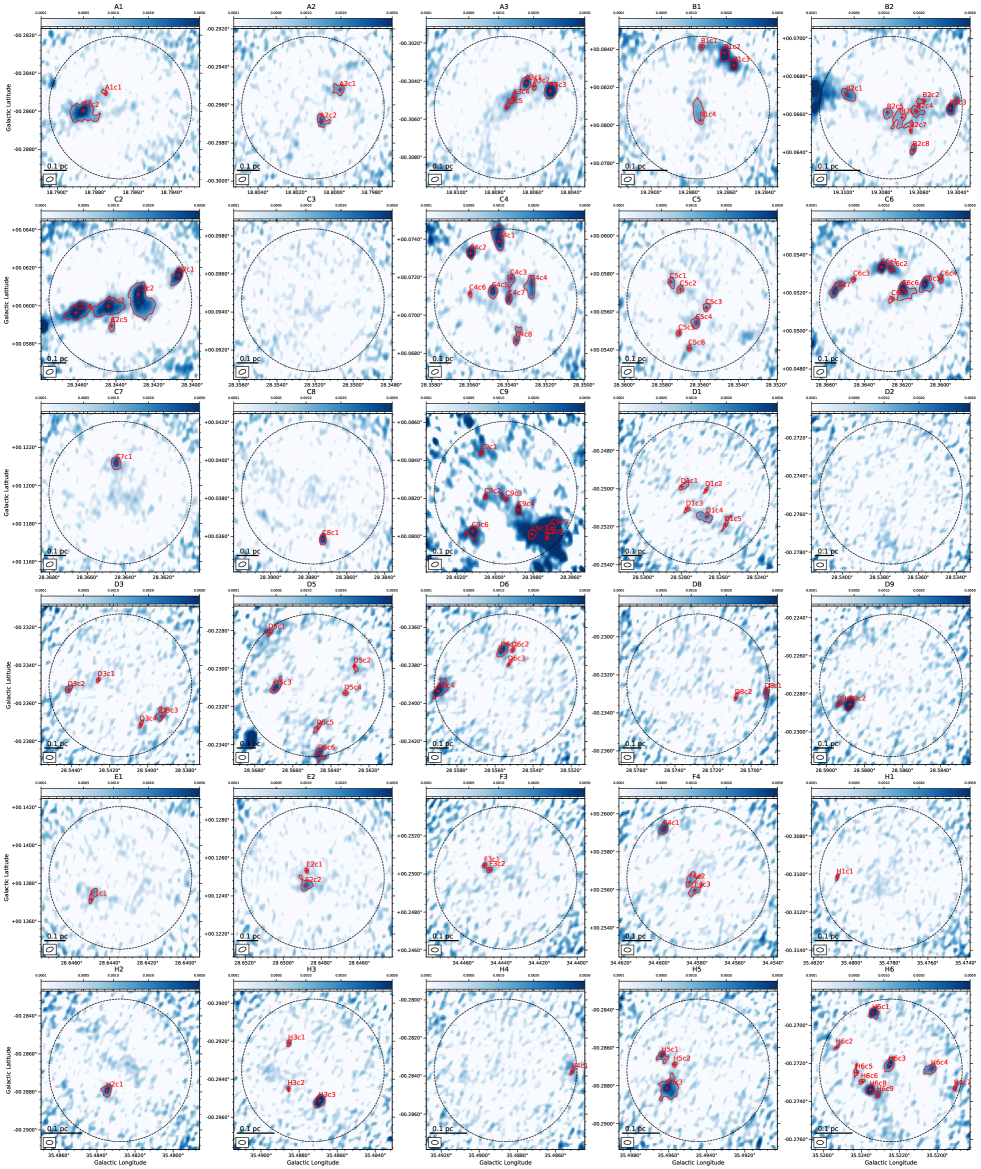
Figure 2: 1.3 mm continuum images of 30 pointings toward IRDC dense clumps (colorbar in Jy beam^-1). The dotted circle in each panel denotes the primary beam. The synthesized beam is shown in the bottom left corner of each panel. The cores identified by the fiducial dendrogram algorithm are marked on the images, with red contours showing “leaf” structures.

3.2 Core Mass Function

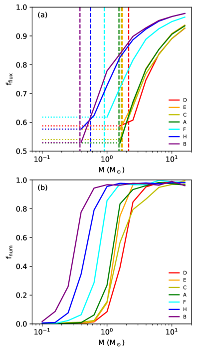
Figure 3: (a) Top: Average (median) flux recovery fractions, $f_{\rm flux}$, versus core mass, $M$, for the dendrogram core finding method as applied to each of the seven IRDCs (solid lines; see legend). Note that our method assumes a constant value of $f_{\rm flux}$ (dotted portion of lines) once an effective minimum is reached as $M$ is reduced (see text). Vertical dashed lines show the mass corresponding to a core that has a flux level of $4\sigma$ at the position of half the beam size, which represents one of the detection threshold criteria, assuming its flux distribution is shaped as the beam. Note that the legend is ordered by cloud distance: IRDC B is the nearest; IRDC D is the most distant. (b) Bottom: Mean value of the number recovery fraction, $f_{\rm num}$, versus core mass, $M$, for the dendrogram core finding method as applied to each of the seven IRDCs (solid lines; see legend).

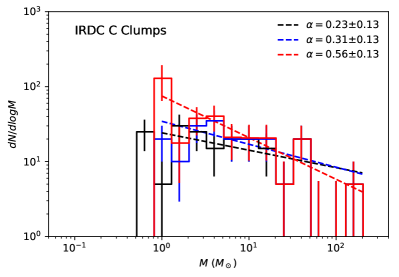
Figure 4: The dendrogram-derived combined CMF of the seven clumps observed in IRDC C. The black histogram shows the original, “raw” CMF. The blue histogram shows the CMF after flux correction and the red histogram shows the final, “true” CMF after then applying number recovery fraction correction. The error bars show Poisson counting errors. The black, blue and red dashed lines show the best power law fit results for the high-mass end ($M\geq 0.79\>M_{\odot}$) of these CMFs, respectively.

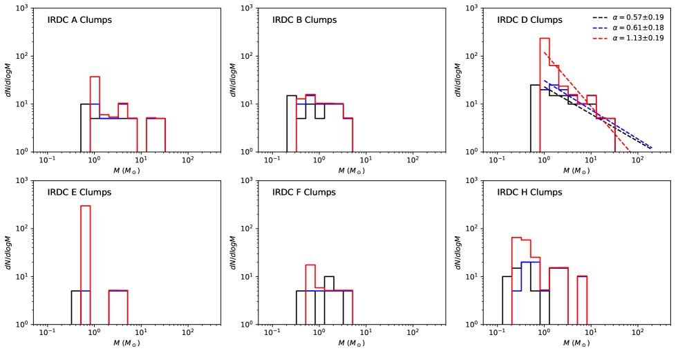
Figure 5: Similar to Figure 4 for IRDC C, the raw (black), flux-corrected (blue) and true (red) CMFs are shown here for IRDCs A, B, D, E, F and H. The black, blue and red dashed lines show the best power law fit results for the high-mass end ($M\geq 0.79\>M_{\odot}$) of the CMF in IRDC D. Other IRDCs are not fit, given their relatively small number of cores.

As described in §2.4, we have estimated flux correction, $f_{\rm flux}$, functions for all the observed regions and these are shown in Figure 3a for the seven IRDCs. Here the values shown are the median of the results for each IRDC in each mass bin (excluding values $f_{\rm flux}>1$, which we attribute to false assignments; and extrapolating with constant values at the low-mass end once an effective minimum is reached in the distribution: at even smaller values of $M$, the median $f_{\rm flux}$ is seen to rise, which we attribute to false assignment to weak image feature, including noise fluctuations). Similar to the results of Paper I for G286, our estimated values of $f_{\rm flux}$ rise from $\sim 0.5$ to 0.6 for $M\lesssim 1\>M_{\odot}$ towards close to unity for $M\gtrsim$ several $M_{\odot}$. The curves are shifted to lower masses for the most nearby IRDCs. Figure 3a also shows for each IRDC the masses corresponding to a core that has a flux level of $4\sigma$ at the position of half the beam size, which represents one of the detection threshold criteria (in this case the most stringent), assuming its flux distribution is shaped as the beam. These mass detection limits range from about 0.4$\>M_{\odot}$ to 2$\>M_{\odot}$, depending on the distance to the cloud. However, we note that these are only approximate limits, since, e.g., the core shape may not be exactly the same as the beam. In particular, less centrally peaked cores will be able to satisfy the area threshold condition at a lower mass.

As also described in §2.4, we then derive the number recovery fraction, $f_{\rm num}$, for the observed regions, again averaging for each IRDC (Fig. 3b). These rise steeply from near zero to near unity as $M$ increases from $\sim 0.2$ to $1\>M_{\odot}$, depending on the distance to the IRDC.

Recall that overall we have identified 107 cores in the seven IRDCs. Cloud C contains the most (37), followed by cloud D (23) and cloud H (18). We will first derive the CMFs for each IRDC separately and then combine them.

The raw (uncorrected) CMF of IRDC C is shown by the black histogram in Figure 4. The mass binning has been chosen to match that used in Paper I, i.e., five bins per dex, with a bin centered on $1\>M_{\odot}$ (and thus also on $10\>M_{\odot}$ and $100\>M_{\odot}$, etc). The error bars on each bin indicate $N^{1/2}$ Poisson counting uncertainties. The CMF after flux correction is shown by the blue histogram: note that cores in the lowest mass bin of the raw CMF are all shifted to higher mass bins. Finally, the number correction is applied to the flux-corrected CMF to derive the final, “true” CMF, shown by the red histogram. Note, its error bars are assumed to be the same fractional size as those found for the blue histogram, i.e., the Poisson errors from this distribution, with no allowance for any additional systematic uncertainty in $f_{\rm num}$. Thus these uncertainties should be treated with caution, i.e., they likely underestimate the true uncertainties.

Following Paper I, we first carry out “simple” power law fitting to CMFs starting from the $1\>M_{\odot}$ bin, i.e., for $M\gtrsim 0.79\>M_{\odot}$. This fitting minimizes differences in the log of $dN/d{\rm log}M$, normalized using the asymmetric Poisson errors. For empty bins, to treat these as effective upper limits, we assume the point is 1 dex lower than the level if the bin had 1 data point and set the upper error bar such that it reaches up to the level if there were 1 data point. For bins that have 1 data point, the lower error bar extends down by 1 dex rather than to minus infinity. As with Paper I, we have verified that the global results are insensitive to the details of how empty bins are treated.

We also apply a maximum likelihood estimation (MLE) method to estimate the power law index (Newman et al. 2005). Let $p(x)dx$ be the fraction of cores with mass between $x$ and $x+dx$. Then $p(x)=Cx^{-(\alpha+1)}$ and $\alpha$ is estimated as

$$\alpha=n\left[\sum_{i=1}^{n}{\rm ln}\frac{x_{i}}{x_{\rm min}}\right]^{-1}$$ (3)

with an uncertainty (confidence interval)

$$\sigma=\frac{\alpha}{\sqrt{n}}.$$ (4)

Here $x_{\rm min}$ is the starting mass of the power law, $x_{i}$ is the mass of each core with mass above $x_{\rm min}$ and $n$ is the number of such cores. We note that this estimate is valid assuming the upper limit (if any) of the distribution is much larger than $x_{\rm min}$. Note also, our fiducial results involve CMFs that have been corrected in logarithmic bins for flux and number incompleteness, so these are used to generate synthetic populations of cores, to which the MLE analysis method is then applied. We generate the corresponding number of random masses uniformly distributed in each mass bin and apply the MLE method. We repeat this for 50 times and then derive the median $\alpha$ and confidence interval $\sigma$.

For IRDC C, with simple power law fitting we derive a value of $\alpha=0.56\pm 0.13$ for the true CMF. The raw and flux-corrected CMFs had power law indices of 0.23 and 0.31, respectively, so we see the effects of these corrections has been to steepen the upper end slope of the CMF, as expected. For the MLE method we find $\alpha=0.48\pm 0.08$, $0.49\pm 0.08$ and $0.75\pm 0.09$ for the raw, flux-corrected and “true” CMF. The slopes derived from the MLE method are slightly steeper than those derived from the linear fitting method within 1.5 combined $\sigma$.

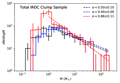
Figure 6: Combined dendrogram-derived CMF from observations of 30 positions covering dense clumps within seven IRDCs. The black histogram shows the original, “raw” CMF. The blue histogram shows the CMF after flux correction and the red histogram shows the final, “true” CMF after then applying number recovery fraction correction. The error bars show Poisson counting errors. The black, blue and red dashed lines show the best power law fit results for the high-mass end ($M\geq 0.79\>M_{\odot}$) of these CMFs, respectively.

In Figure 5 we show the equivalent CMFs for the six other IRDCs, most of which are very sparsely sampled. We also carry out power-law fitting for IRDC D (23 cores). From simple power law fitting we derive a value of $\alpha=1.13\pm 0.19$ for the true CMF. This is significantly steeper than the result for IRDC C, however, it driven mostly by the lowest mass bin, i.e., $\sim 1\>M_{\odot}$, for which the completeness correction is about a factor of 10. Due to potential uncertainties associated with this correction, as we discuss below, we will consider CMFs down to two mass thresholds, i.e., cases of including and excluding this mass bin.

Next, in Figure 6, we show the combined CMFs for the entire sample of seven IRDCs. The raw, flux-corrected and “true” CMFs (black, blue and red histograms, respectively) are obtained by simple addition of the equivalent CMFs for each individual IRDC. Note that the Poisson errors are now reduced. Note also, however, there are still two empty bins near $100\>M_{\odot}$ and only one core more massive that this. At the low-mass end, the CMFs of the seven individual IRDCs all have detections down to or below the bin centered on $M=1\>M_{\odot}$, which is approximately the detection threshold of Cloud D, the farthest cloud.

For the raw, flux-corrected and “true” CMFs, with simple fitting we then derive power law indices for $M>0.79\>M_{\odot}$ of $\alpha=0.50\pm 0.10$, $0.49\pm 0.09$ and $0.86\pm 0.11$, respectively. For MLE, we derive $\alpha=0.61\pm 0.07$, $0.63\pm 0.07$ and $1.02\pm 0.08$ for these three cases, respectively. Again, the slopes derived from the MLE method are slightly steeper than those derived from the linear fitting method within 1.5 combined $\sigma$. If we only fit to the true CMF starting from the next bin above $1\>M_{\odot}$ (i.e., allowing for the possibility that IRDC D is artificially distorting the low-end CMF), then we derive $\alpha=0.70\pm 0.13$ for the true CMF. The MLE analysis yields $\alpha=0.83\pm 0.09$.

While we prefer the dendrogram algorithm as our fiducial method of identifying cores, since it is a hierarchical method that we consider better at separating cores from a surrounding background clump environment (see §2.2 and Paper I), for completeness we also evaluate the CMF as derived from the clumpfind algorithm. With the fiducial parameters (i.e., a $4\sigma$ noise threshold, $3\sigma$ step size, minimum area of 0.5 beams; see Paper I), we find 120 cores with masses from 0.150 to $286\>M_{\odot}$. After flux and number recovery corrections on each IRDC, for the combined “true” CMF we derive a high-mass end ($M>0.79\>M_{\odot}$) power law index of $\alpha=0.86\pm 0.11$ with simple fitting and $1.02\pm 0.08$ with MLE fitting. The first of these values is coincidentally the same (within the first two significant figures) as that derived from the dendrogram analysis. These results indicate that for our ALMA observations of IRDC clumps, the resulting core properties are not that sensitive to whether dendrogram or clumpfind is used as the identification algorithm. This contrasts with the results of Paper I for G286 (for the case of 1.5″resolution), which found a value of $\alpha=1.12\pm 0.18$ for dendrogram and $\alpha=0.49\pm 0.12$ for clumpfind. We expect that this difference is due, at least in part, to the observation of G286 utilizing both the 12-m and 7-m arrays, so that a larger range of scales are recovered. Thus more emission from the surrounding protocluster clump material is detected in G286, readily apparent from Figures 1 & 2 of Paper I, in comparison to our images of the IRDC clumps (Fig. 2). Since most of the larger-scale emission is resolved out in our IRDC observations (an approximate comparison with BGPS data of the clumps assuming a dust spectra index of 3.5 finds typical flux recovery of $\sim 20\%$ [see §2.1]), one then expects clumpfind results to be closer to those derived from dendrogram.

We examine whether the CMF we measure in IRDC environments is consistent with a Sapleter distribution ($\alpha=1.35$). We can already infer from our measurements of $\alpha=0.70\pm 0.13$ (or with MLE $\alpha=0.83\pm 0.09$) for the true CMF at $M>1.26\>M_{\odot}$, that the result differs from Salpeter by about $5.0\sigma$ (or $5.8\sigma$ for MLE). However, it is not known if the uncertainties in these parameters, especially given systematic uncertainties, will follow a simple gaussian distribution. More generally we compare the IRDC core population (including allowance for completeness corrections) with an idealized large (e.g., $1,000$, but result is independent of this size for large enough numbers) population of cores that follow the Salpeter distribution over the same mass range. We carry out a Kolmogorov-Smirnov (KS) test with synthetic populations of cores by generating the corresponding number of random masses uniformly distributed in each mass bin and repeat for 50 times. We find that the median $p$ value, which indicates the probability that these distributions are consistent with the same parent distribution, is $\lesssim 10^{-4}$. Thus we conclude that our estimated CMF in IRDC environments is top heavy compared to Salpeter. Such a conclusion has also recently been reported in the more evolved “mini-starburst” W43 region by Motte et al. (2018).

3.3 Comparison to G286

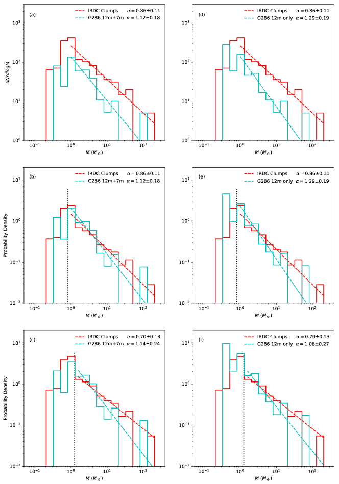
Figure 7: (a) Top: Flux and number-corrected “true” dendrogram-derived CMF of IRDC clumps (red histogram) compared with the same CMF derived from G286 in Paper I (cyan histogram). The simple power law fits to $M\geq 0.79\>M_{\odot}$ are also indicated. (b) Middle: As (a), but now showing CMFs normalized by the number of cores estimated, after completeness corrections, to have $M\geq 0.79\>M_{\odot}$, i.e., 176 cores in the IRDC Clumps and 66 cores in G286 after completeness corrections. This mass threshold is indicated by the vertical black dotted line. (c) Bottom: As (a), but now showing CMFs normalized by the number of cores with $M\geq 1.26\>M_{\odot}$, i.e., 91 cores in the IRDC Clumps and 39 cores in G286 after completeness corrections. This mass threshold is indicated by the vertical black dotted line. Simple power law fits for this mass range are also shown. (d) Top: As (a), but comparing to results from G286 12m-only data. (e) Middle: As (b), but comparing to results from G286 12m-only data (61 cores in G286 after completeness corrections are used for the normalization). (f) Bottom: As (c), but comparing to results from G286 12m-only data (29 cores in G286 after completeness corrections are used for the normalization).

Here we present a detailed comparison of our fiducial dendrogram-derived CMF in IRDC clumps with that measured in the more evolved G286 protocluster in Paper I. We have already noted and summarize again that there are some unavoidable differences in our observational data and analysis methods compared to Paper I. In addition to the primary beam effect mentioned in §2.2, our observations do not include the 7m array and so lack sensitivity to larger-scale structures. Also, we compile a CMF from observations of multiple clouds that are at a range of distances, whereas Paper I studied a single protocluster, G286, at a single distance of 2.5 kpc. We will compare to the results of the 1.5″resolution analysis of Paper I, since, as discussed below, this is a better match to our observations of typically more distance IRDCs at $\sim$1″resolution.

Figure 7a shows shows the dendrogram-derived flux and number-corrected, i.e., “true” CMFs from the IRDC clumps and G286 together. Figure 7b shows these same CMFs, but now normalized by the number of cores they contain in the $1\>M_{\odot}$ mass bin and greater, i.e., $M\geq 0.79\>M_{\odot}$. Figure 7c shows the CMFs normalized by the number of cores they have with $M\geq 1.26\>M_{\odot}$, i.e., in case the $1\>M_{\odot}$ mass bin is adversely affected by systematic errors, especially from IRDC D. This panel also displays the power law indices that result from simple fitting over this slightly higher mass range.

The potential systematic difference resulting from the lack of 7-m array data for the IRDC clumps needs to be considered. Paper I found that the CMF derived without 7-m array data in G286 is steeper by about 0.1. Accounting for this effect thus may accentuate the difference between the IRDC clump and G286 CMFs. We proceed to re-analyze the G286 data but now excluding the 7m-array data, which gives the fairest comparison with our IRDC clump observations. These results are shown in Figure 7 d, e and f.

We carry out a KS test of the high-mass end CMFs to see if the distributions identified in IRDC clumps and in G286 (with 12m only data) are consistent with being drawn from the same parent distribution. For the case of CMFs in the range $M\geq 0.79\>M_{\odot}$, the resulting $p$ value is 0.42. For the distributions in the range $M\geq 1.26\>M_{\odot}$, the KS test yields $p=0.23$. Thus these results indicate that the distributions are possibly consistent with one another, in spite of the apparent differences in their power law indices. If we were to boost the number of cores by a factor of 5 and keeping the same distributions, then the $p$ values would become smaller to the point that they would be inconsistent with one another. This test indicates that such an increase in sample size is needed to be able to distinguish between CMFs that have a difference in $\alpha$ of about 0.4.

One potential systematic effect resulting from differences between the observations is that G286 is at a single distance of $d=2.5\>$kpc and was observed with a resolution of about 1.5″and with a noise level of 0.5 mJy beam^-1, while the IRDCs, are observed with a resolution of $\sim 1\arcsec$ and noise level of $\sim 0.2$ mJy beam^-1. Paper I also presented results for 1.0″resolution and with a noise level of 0.45 mJy beam^-1, which yields $\alpha=1.24\pm 0.17$ for $M\geq 0.79\>M_{\odot}$, however, we have decided to focus on the lower resolution resolution results, given that the IRDCs span a range of distances from 2.4 to 5.7 kpc, but with IRDC C at 5 kpc and IRDC D at 5.7 kpc contributing a large fraction of the sample so that the average distance of the IRDC cores is 4.4 kpc. Thus in the end the effective linear resolutions are similar (within about 15%) for the average IRDC core and that achieved in G286. Overall the mass sensitivities are also quite similar between the two observations and the completeness correction factors are relatively modest, at least for $M\geq 1.26\>M_{\odot}$.

4 Discussion and Conclusions

We have measured the CMF in a sample of about 30 IRDC clumps, including accounting for flux and number recovery incompleteness factors. With simple fitting, we derived high-end power law indices of $\alpha\simeq 0.86\pm 0.11$ for $M\geq 0.79\>M_{\odot}$ and $\alpha\simeq 0.70\pm 0.13$ for $M\geq 1.26\>M_{\odot}$. An MLE analysis yielded similar values. These results indicate a CMF that is top heavy compared the standard Salpeter distribution with $\alpha=1.35$.

To reduce the potential effects of systematic uncertainties, we have compared the above results to the CMF derived with similar methods in the more evolved protocluster G286 (Paper I). From the considerations of §3, we expect that the most reliable comparison is for the higher mass range of the CMF, $M\geq 1.26\>M_{\odot}$, for which we have found $\alpha=1.08\pm 0.27$ for G286 when only the 12m-array data are analyzed. These results thus indicate only a hint of a potential variation in the high-mass end of the CMF between the Galactic environments of IRDC clumps (i.e., early stage, high pressure centers of protoclusters) and G286, i.e., a more evolved protocluster that is sampled more globally, i.e., both central and outer regions. One of the main factors limiting our ability to distinguish the distributions is the relatively small number of cores in each of the samples used in this direct comparison. Increasing the sample by about a factor of 5 is expected to enable these distributions to be reliably distinguished, if they maintain their currently observed forms.

Overall, the values of power law index of the CMF derived in G286 is similar to that of the Salpeter stellar IMF, i.e., $\alpha=1.35$, while that in the IRDC clumps is shallower, indicating relatively more massive cores are present. This may indicate that massive stars are more likely to form in high mass surface density, high pressure regions of IRDCs. Such a difference in the CMF and resulting IMF could potentially be caused by a number of different physical properties of the gas that vary systematically between the regions. On the one hand, the higher density, higher pressure regions of IRDC clumps is expected to lead to a smaller Bonnor-Ebert mass, which would also take a value $\ll 1\>M_{\odot}$ (see, e.g., McKee & Tan 2003). The fact that we see evidence for a more top-heavy CMF indicates that thermal pressure is not the main factor resisting gravity in setting core masses in these environments, which would then indicate that some combination of increased turbulence and/or magnetic field support is present in IRDC clumps.

Note that IRDC clumps are cold regions, so that extra thermal heating of the ambient environment from radiative feedback from surrounding lower-mass stars, as proposed in the model of Krumholz & McKee (2008), is not expected to be greater here compared to more evolved stages as represented by G286. However, localized heating of the core from the protostar itself is expected to be higher in higher mass surface density environments, if powered mostly by accretion (Zhang & Tan 2015). At the moment we do not have any direct indication if the localized temperatures of cores are higher in the IRDC clumps compared to G286. Note, if localized IRDC core temperatures were systematically higher than in G286, then we would have overestimated their masses. If this effect is greater for the more luminous mm cores and is systematically greater in the IRDC sample compared to G286, then this would make their intrinsic CMFs more similar. Such considerations highlight additional potential systematic effects due to temperature or dust opacity variations that need to be treated as caveats to our results, and indeed all results of CMFs derived from mm dust emission when individual core temperature and opacity data are not available.

Comparing with previous studies in IRDCs, our relatively flat high-mass end power law index is consistent with the results of Ragan et al. (2009), although they probed a different mass range of 30 to 3,000$\>M_{\odot}$ and used different methods, i.e., MIR extinction, which is subject to a variety of systematic uncertainties (Butler & Tan 2012), including foreground corrections that effect lower column density regions and “saturation” effects at high optical depths causing the mass in high column density regions to be underestimated. Zhang et al. (2015) also found a relative lack of lower-mass cores compared to the Salpeter (1955) distribution, but their sample size was relatively small (only 38 cores selected in a single small, $\sim 0.5$ pc region) and they did not carry out completeness corrections. Still, their results do illustrate the effects of using higher angular resolution (by about a factor of two, i.e., $\sim 0.8\arcsec$), better sensitivity (by about a factor of three, i.e., $1\sigma$ rms of 75$\>\rm\mu$Jy), but with more limited sensitivity to larger scale structures (given a more extended configuration of ALMA was employed) compared to our current study. The 5 cores we identify in the C2 clump are further decomposed into 34 cores by Zhang et al. (2015), i.e., the bulk of their sample, in their analysis of core identification, which is based on the dendrogram method, but also supplemented by dendrogram-guided Gaussian fitting of additional structures. On the other hand, Ohashi et al. (2016) found a steeper power law index for the pre-stellar CMF derived in their study (28 cores in IRDC G14.225-0.506 found by 3 mm continuum emission), although the uncertainty in their result is large ($\alpha\simeq 1.6\pm 0.7$) and, again, their methods differ from ours, especially the lack of completeness corrections for flux and number. Motte et al. (2018) have recently studied the 1.3 mm dust continuum derived CMF in the W43-MM1 “mini-starburst region”, finding $\alpha=0.90\pm 0.06$ for $M>1.6\>M_{\odot}$, based on a sample of 105 cores. We note they used different methods of core identification, i.e., the getsources algorithm (Men’shchikov et al. 2012), but also carried out a visual inspection step of removing cores that were “too extended, or whose ellipticity is too large to correspond to cores, or that are not centrally-peaked”, so a direct comparison with our results is not as meaningful as our comparison to the G286 protocluster.

In summary, we see that quantitative direct comparison of our results with these previous studies is not particularly useful given the differences in the data and methods used to identify cores and estimate CMFs. We thus emphasize that, in addition to finding a more top heavy CMF compared to the Salpeter distribution, our main result for a hint of a potential variation in the CMF in different environments is based on the comparison with our Paper I study of G286, which used more similar data and methods.

Future progress in this field can take several directions. First, as discussed above, much larger samples of cores in these types of environments are needed. Second, a wider range of Galactic environments need to be probed. Third, the CMF should be probed to lower masses to better determine the location of any peak. This will require higher sensitivity and higher angular resolution observations. Such observations will also likely change the shape of the high-mass end of the CMF by sometimes breaking up more massive “cores” into smaller units. Fourth, better constraints on potential systematic effects related to mass determination from mm continuum flux are needed, especially by individual temperature measurements of the cores. Fifth, the evolutionary stage of the cores should be determined, i.e., protostellar mass to core envelope mass, including determining if cores are pre-stellar, i.e., via astrochemical indicators or via an absence of outflow indicators or concentrated continuum emission. Such information is needed to better determine how the CMF and IMF are actually established in protocluster environments, as discussed by Offner et al. (2014).

References

- Aguirre, et al. (2011) Aguirre, J. E., Ginsburg, A. G., Dunham, M. K., et al. 2011, The Astrophysical Journal Supplement Series, 192, 4
- Alves et al. (2007) Alves, J., Lombardi, M., & Lada, C. J. 2007, A&A, 462, L17
- André et al. (2010) André, P., Men’shchikov, A., Bontemps, S., et al. 2010, A&A, 518, L102
- Bastian et al. (2010) Bastian, N., Covey, K. R., & Meyer, M. R. 2010, ARA&A, 48, 339
- Beuther & Schilke (2004) Beuther, H. & Schilke, P. 2004, Science, 303, 1167.
- Butler & Tan (2009) Butler, M. J., & Tan, J. C. 2009, ApJ, 696, 484
- Butler & Tan (2012) Butler, M. J., & Tan, J. C. 2012, ApJ, 754, 5
- Carey, et al. (2009) Carey, S. J., Noriega-Crespo, A., Mizuno, D. R., et al. 2009, Publications of the Astronomical Society of the Pacific, 121, 76.
- Caselli & Ceccarelli (2012) Caselli, P., & Ceccarelli, C. 2012, A&A Rev., 20, 56
- Cheng et al. (2018) Cheng, Y., Tan, J. C., Liu, M., et al. 2018, ApJ, 853, 160
- Draine (2011) Draine B. T. 2011, Physics of the Interstellar and Intergalactic Medium (Princeton: Princeton Univ. Press)
- Ginsburg, et al. (2013) Ginsburg, A., Glenn, J., Rosolowsky, E., et al. 2013, The Astrophysical Journal Supplement Series, 208, 14
- Kong et al. (2017) Kong, S., Tan, J. C., Caselli, P., et al. 2017, ApJ, 834, 193
- Könyves, et al. (2015) Könyves, V., André, P., Men’shchikov, A., et al. 2015, A&A, 584, A91
- Krumholz & McKee (2008) Krumholz, M. R., & McKee, C. F. 2008, Nature, 451, 1082
- Lim et al. (2016) Lim, W., Tan, J. C., Kainulainen, J., Ma, B., & Butler, M. J. 2016, ApJ, 829, L19
- McKee & Tan (2003) McKee, C. F., & Tan, J. C. 2003, ApJ, 585, 850
- Men’shchikov, et al. (2012) Men’shchikov, A., André, P., Didelon, P., et al. 2012, A&A, 542, A81.
- Motte, et al. (2018) Motte, F., Nony, T., Louvet, F., et al. 2018, Nature Astronomy, 50
- Newman (2005) Newman, M. E. J. 2005, Contemporary Physics, 46, 323
- Offner et al. (2014) Offner, S. S. R., Clark, P. C., Hennebelle, P., et al. 2014, Protostars and Planets VI, 53
- Ohashi et al. (2016) Ohashi, S., Sanhueza, P., Chen, H.-R. V., et al. 2016, ApJ, 833, 209
- Ossenkopf & Henning (1994) Ossenkopf V. & Henning T. 1994, A&A, 291, 943
- Pillai et al. (2006) Pillai, T., Wyrowski, F., Carey, S. J., & Menten, K. M. 2006, A&A, 450, 569
- Ragan et al. (2009) Ragan, S. E., Bergin, E. A., & Gutermuth, R. A. 2009, ApJ, 698, 324
- Rathborne et al. (2006) Rathborne, J. M., Jackson, J. M., & Simon, R. 2006, ApJ, 641, 389
- Rosolowsky et al. (2008) Rosolowsky, E. W., Pineda, J. E., Kauffmann, J. & Goodman, A. A. 2008, ApJ, 679, 1338
- Salpeter (1955) Salpeter, E. E. 1955, ApJ, 121, 161
- Sokolov et al. (2017) Sokolov, V., Wang, K., Pineda, J. E., et al. 2017, A&A, 606, A133
- Tan et al. (2013) Tan, J. C., Kong, S., Butler, M. J. et al. 2013, ApJ, 779, 96
- Tan et al. (2014) Tan, J. C., Beltrán, M. T., Caselli, P., et al. 2014, Protostars and Planets VI, 149
- Tan, et al. (2016) Tan, J. C., Kong, S., Zhang, Y., et al. 2016, ApJ, 821, L3.
- Williams et al. (1994) Williams, J. P., de Geus, E. J., & Blitz, L. 1994, ApJ, 428, 693
- Zhang & Tan (2015) Zhang, Y., & Tan, J. C. 2015, ApJ, 802, L15
- Zhang et al. (2015) Zhang, Q., Wang, K., Lu, X., & Jiménez-Serra, I. 2015, ApJ, 804, 141