Optimal Inference with a Multidimensional Multiscale Statistic

Abstract

We observe a stochastic process $Y$ on $[0,1]^{d}$ ($d\geq 1$) satisfying $dY(t)=n^{1/2}f(t)dt$ + $dW(t)$, $t\in[0,1]^{d}$, where $n\geq 1$ is a given scale parameter (‘sample size’), $W$ is the standard Brownian sheet on $[0,1]^{d}$ and $f\in L_{1}([0,1]^{d})$ is the unknown function of interest. We propose a multivariate multiscale statistic in this setting and prove its almost sure finiteness; this extends the work of Dümbgen and Spokoiny, [10] who proposed the analogous statistic for $d=1$. We use the proposed multiscale statistic to construct optimal tests for testing $f=0$ versus (i) appropriate Hölder classes of functions, and (ii) alternatives of the form $f=\mu_{n}\mathbb{I}_{B_{n}}$, where $B_{n}$ is an axis-aligned hyperrectangle in $[0,1]^{d}$ and $\mu_{n}\in{\mathbb{R}}$; $\mu_{n}$ and $B_{n}$ unknown. In the process we generalize Theorem 6.1 of Dümbgen and Spokoiny, [10] about stochastic processes with sub-Gaussian increments on a pseudometric space, which is of independent interest.

arXiv:0000.0000

and

t2Supported by NSF grant DMS-17-12822 and AST-16-14743.

1 Introduction

Let us consider the following continuous multidimensional white noise model:

$${\small Y(t_{1},\ldots,t_{d})=\sqrt{n}\int_{0}^{t_{1}}\ldots\int_{0}^{t_{d}}f(s_{1},\ldots,s_{d})\;ds_{d}\ldots ds_{1}+W(t_{1},\ldots,t_{d}),}$$ (1.1)

for $(t_{1},\ldots,t_{d})\in[0,1]^{d}$ ($d\geq 1$), where $\{Y(t_{1},\ldots,t_{d}):(t_{1},\ldots,t_{d})\in[0,1]^{d}\}$ is the observed data, $f\in L_{1}([0,1]^{d})$ is the unknown (regression) function of interest and $W(\cdot)$ is the unobserved $d$-dimensional Brownian sheet (see Definition 6.1), and $n$ is a known scale parameter. Estimation and inference in this model is closely related to that of nonparametric regression based on sample size $n$. We work with this white noise model as this formulation is more amiable to rescaling arguments; see e.g., Donoho and Low, [9], Dümbgen and Spokoiny, [10], Carter, [5].

In this paper we develop optimal tests (in an asymptotic minimax sense) based on a newly proposed multidimensional multiscale statistic (i.e., $d\geq 1$) for testing:

• $f=0$ versus a Hölder class of functions with unknown degree of smoothness;

• $f=0$ against alternatives of the form $f=\mu_{n}\mathbb{I}_{B_{n}}$, where $B_{n}$ is an unknown hyperrectangle in $[0,1]^{d}$ with sides parallel to the coordinate axes (i.e., axis-aligned) and $\mu_{n}\in{\mathbb{R}}$ is unknown (for different regimes of $\mu_{n}$ and $B_{n}$).

Scenario (i) arises quite often in nonparametric regression where the goal is to test whether the underlying $f$ is 0 versus $f\neq 0$ with unknown smoothness; see e.g., Lepski and Tsybakov, [30], Horowitz and Spokoiny, [18], Ingster and Sapatinas, [23] and the references therein. Our proposed multiscale statistic, which extends the work of Dümbgen and Spokoiny, [10] that considered the analogous statistic for $d=1$, leads to rate optimal detection in this problem. Moreover, with the knowledge of the smoothness of the underlying $f$, we construct a asymptotically minimax test which even attains the exact separation constant (see Section 1.2 for formal definitions and related concepts).

Setting (ii) is a prototypical problem in signal detection — an unknown (constant) signal spread over an unknown hyperrectangular region — and the goal is to detect the presence of such a signal; see e.g., Arias-Castro et al., [3], Chan, [6], Walther, [42], Frick et al., [12], Butucea et al., [4], Chan and Walther, [7], Glaz and Zhang, [15], König et al., [28] for a plethora of examples and applications.

Although several minimax rate optimal tests have been proposed in the literature for this problem (see e.g., Arias-Castro et al., [3], Chan, [6], Butucea et al., [4] and König et al., [28]), as far as we are aware, our proposed multiscale test is the only test that attains the exact separation constant — this leads to simultaneous optimal detection of signals both at small and large scales.

We first motivate and introduce our multiscale statistic below (Section 1.1) and briefly describe the asymptotic minimax testing framework and our main optimality results in Section 1.2.

1.1 Multiscale statistic when $d\geq 1$

To motivate our multiscale statistic let us first look at the following testing problem:

$$H_{0}:f=0\quad\mbox{ versus }\quad H_{1}:f\neq 0\in\mathbb{H}_{\beta,L},$$ (1.2)

where $\mathbb{H}_{\beta,L}$ is the Hölder class of function with parameters $\beta>0$ and $L>0$. For $\beta\in(0,1]$ and $L>0$ the Hölder class $\mathbb{H}_{\beta,L}$ is defined as

$$\mathbb{H}_{\beta,L}:=\Big{\{}f\in L_{1}([0,1]^{d}):|f(x)-f(y)|\leq L\left\lVert x-y\right\rVert^{\beta}\mbox{ for all }x,y\in[0,1]^{d}\Big{\}}.$$ (1.3)

For $\beta>1$ the Hölder class $\mathbb{H}_{\beta,L}$ is defined similarly; see Definition 6.2.

Our multiscale statistic is based on the idea of kernel averaging. Suppose that $\psi:\mathbb{R}^{d}\to{\mathbb{R}}$ is a measurable function such that (i) $\psi$ is $0$ outside $[-1,1]^{d}$; (ii) $\psi\in L_{2}({\mathbb{R}}^{d})$, i.e., $\int_{{\mathbb{R}}^{d}}\psi^{2}(x)dx<\infty$; (iii) $\psi$ is of bounded (HK)-variation (see Definition 6.3); and (iv) $\int_{{\mathbb{R}}^{d}}\psi(x)dx>0$. We call such a function a kernel. For any $h:=(h_{1},\ldots,h_{d})\in(0,1/2]^{d}$ we define

$$A_{h}:=\{t\in\mathbb{R}^{d}:h_{i}\leq t_{i}\leq 1-h_{i}\;\;\mbox{ for }i=1,\ldots,d\}.$$ (1.4)

For any $t\in A_{h}$ we define the centered (at $x$) and scaled kernel function $\psi_{t,h}:[0,1]^{d}\to{\mathbb{R}}$ as

$$\psi_{t,h}(x):=\psi\left(\frac{x_{1}-t_{1}}{h_{1}},\ldots,\frac{x_{d}-t_{d}}{h_{d}}\right),\quad\mbox{for }\;x=(x_{1},\ldots,x_{d})\in[0,1]^{d}.$$ (1.5)

For a fixed $t\in A_{h}$ we can construct a kernel estimator $\hat{{f_{h}}}(t)$ of $f(t)$ based on the data process $Y(\cdot)$ as

$$\hat{{f_{h}}}(t):=\frac{1}{n^{1/2}(\Pi_{i=1}^{d}h_{i})\langle 1,\psi\rangle}\int_{[0,1]^{d}}\psi_{t,h}(x)dY(x),$$

where for any two functions $g_{1},g_{2}\in L_{2}({\mathbb{R}}^{d})$, we define $\langle g_{1},g_{2}\rangle:=\int_{{\mathbb{R}}^{d}}g_{1}(x)g_{2}(x)dx.$ We consider the normalized version of the above kernel estimator $\hat{{f_{h}}}(t)$:

$$\hat{\Psi}(t,h):=\frac{1}{(\Pi_{i=1}^{d}h_{i})^{1/2}\left\lVert\psi\right\rVert}\int_{[0,1]^{d}}\psi_{t,h}(x)dY(x),$$ (1.6)

where $\left\lVert\psi\right\rVert^{2}:=\int_{{\mathbb{R}}^{d}}\psi^{2}(x)dx<\infty$. We can use $\hat{\Psi}(t,h)$ to test

$$H_{0}:f(t)=0\quad\mbox{ versus }\quad H_{1}:f(t)\neq 0$$

where we would reject the null hypothesis for extreme values of $\hat{\Psi}(t,h)$. So, a naive approach to testing (1.2) could be to consider $\sup_{t\in A_{h}}|\hat{\Psi}(t,h)|$. As this test statistic crucially depends on the choice of the smoothing bandwidth vector $h$, an approach that bypasses the choice of the tuning parameter $h$ and also combines information at various bandwidths would be to consider the test statistic

$$\sup_{h>0}\sup_{t\in A_{h}}|\hat{\Psi}(t,h)|,$$ (1.7)

where $h>0$ is a short-hand for $h\in(0,\infty)^{d}$. However, under the null hypothesis

$$\sup_{h>0}\sup_{t\in A_{h}}|\hat{\Psi}(t,h)|=\infty\qquad\mbox{almost surely (a.s.).}$$

This is because, for a fixed scale $h$, $\sup_{t\in A_{h}}|\hat{\Psi}(t,h)|=$ $O_{p}(\sqrt{2\log(1/(2^{d}h_{1}\cdots h_{d}))})$; see Giné and Guillou, [13]. Thus, to use the above approach to construct a valid test for (1.2) we need to put the test statistics $\sup_{t\in A_{h}}|\hat{\Psi}(t,h)|$ at different scales (i.e., $h$) in the same footing — this leads to the following definition of the multiscale statistic in $d$-dimensions:

$$T(Y,\psi):=\sup_{h\in(0,1/2]^{d}}\sup_{t\in A_{h}}\frac{\lvert\hat{\Psi}(t,h)\rvert-\Gamma(2^{d}h_{1}\ldots h_{d})}{D(2^{d}h_{1}\ldots h_{d})}$$ (1.8)

where $\Gamma,D:(0,1]\to(0,\infty)$ are two functions defined as

$$\Gamma(r):=(2\log(1/r))^{1/2}$$

and

$$D(r):=(\log(e/r))^{-1/2}\log\log(e^{e}/r).$$

In Theorem 2.1, a main result in this paper, we show that the above multivariate multiscale statistic $T(Y,\psi)$ is well-defined and finite a.s. for any kernel function $\psi$, when $f\equiv 0$. This result immediately extends the main result of Dümbgen and Spokoiny, [10, Theorem 2.1] beyond $d=1$. Although there has been several proposals that extend the definition and the optimality properties of the multiscale statistic of Dümbgen and Spokoiny, [10] beyond $d=1$ (see e.g., König et al., [28], Walther, [42], Chan and Walther, [7]), we believe that our proposed multiscale statistic is the right generalization. Further, the exact form of $T(Y,\psi)$ leads to optimal tests for (1.2) and other alternatives (which the other competing procedures do not necessarily yield; see Remarks 2.3 and 3.4 for more details).

To show the finiteness of the proposed multiscale statistic we prove a general result about a stochastic process with sub-Gaussian increments (Theorem 2.2) on a pseudometric space which may be of independent interest. This result has the same conclusion as that of Dümbgen and Spokoiny, [10, Theorem 6.1] but assumes a weaker condition on the packing numbers of the pseudometric space on which the stochastic process is defined. This weaker condition on the packing numbers is crucial to the proof of Theorem 2.1; see Remark 2.1 where we compare our result with the existing result of Dümbgen and Spokoiny, [10, Theorem 6.1]. Moreover, Lemma 2.1 gives a tighter bound on the packing numbers of the pertinent (to our application) pseudometric space, which we believe is also new; see Remarks 2.2 and 2.3 where we compare our result with some relevant recent work.

1.2 Optimality of the multiscale statistic

Before we describe our main results let us first introduce the asymptotic minimax hypothesis testing framework. There is an extensive literature on nonparametric testing of the simple hypothesis $\{0\}$. As a staring point we refer the readers to Ingster and Suslina, [24]. In the nonparametric setting it is usually assumed that $f$ belongs to a certain class of functions $\mathbb{F}$ and its distance from the null function $f=0$ is defined by a seminorm $\left\lVert\cdot\right\rVert$. In this setting, given $\alpha\in(0,1)$, the goal is to find a level $\alpha$ test $\phi_{n}$ (i.e., ${\mathbb{E}}_{0}[\phi_{n}(Y)]\leq\alpha$) such that

$$\inf_{g\in\mathbb{F}:\left\lVert g\right\rVert\geq\delta\rho_{n}}{\mathbb{E}}_{g}[\phi_{n}(Y)]$$ (1.9)

is as large as possible for some $\delta>0$ and $\rho_{n}>0$ where $\rho_{n}\to 0$ as $n\to\infty$ ($\rho_{n}$ is a function of the sample size $n$); in the above notation ${\mathbb{E}}_{g}$ denotes expectation under the alternative function $g$. However, it can be shown that given $\mathbb{F}$ and $\left\lVert\cdot\right\rVert$, the constants $\delta$ and $\rho_{n}$ cannot be chosen arbitrarily if one wants to have a statistically meaningful framework (see the survey papers Ingster, 1993a [20], Ingster, 1993b [21], Ingster, 1993c [22] for $d=1$ and Ingster and Sapatinas, [23] for $d>1$). It turns out that if $\delta\rho_{n}$ is too small then it is not possible to test the null hypothesis with nontrivial asymptotic power (i.e., the infimum in (1.9) cannot be strictly larger than $\alpha+o(1)$). On the other hand if $\delta\rho_{n}$ is very large many procedures can test $f\equiv 0$ with significant power (i.e., the infimum in (1.9) goes to $1$ as $n\to\infty$).

The hypothesis testing problem then reduces to: (a) finding the largest possible $\delta\rho_{n}$ such that no test can have nontrivial asymptotic power (i.e., under the alternative $f$ such that $\left\lVert f\right\rVert\leq\delta\rho_{n}$, the asymptotic power is less than or equal to the level $\alpha$), and (b) trying to construct test procedures that can detect signals $f$, with $\left\lVert f\right\rVert\geq\delta\rho_{n}$, with considerable power (power going to $1$ as $n\to\infty$). More specifically, $\delta$ and $\rho_{n}$ are defined such that $\delta\rho_{n}$ is the largest for which, for all $\epsilon>0$, we have

$$\sup_{\phi_{n}}\limsup_{n\to\infty}\inf_{g\in\mathbb{F}:\left\lVert g\right\rVert\geq(1-\epsilon)\delta\rho_{n}}{\mathbb{E}}_{g}[\phi_{n}(Y)]\leq\alpha,$$

where the supremum is taken over all sequence of level $\alpha$ tests $\phi_{n}$. In this case $\rho_{n}$ is called the minimax rate of testing and $\delta$ is called the exact separation constant (see Lepski and Tsybakov, [30], Ingster and Stepanova, [19] for more details about minimax testing). On the other hand, we want to find a test $\tilde{\phi}_{n}$ such that

$$\lim_{n\to\infty}\inf_{g\in\mathbb{F}:\left\lVert g\right\rVert\geq(1+\epsilon)\delta\rho_{n}}{\mathbb{E}}_{g}[\tilde{\phi}_{n}(Y)]=1.$$

In such a scenario, $\tilde{\phi}_{n}$ is called an asymptotically minimax test. Here we would also like to point out that if there exists a test $\hat{\phi}_{n}$ and a constant $\hat{\delta}>\delta$ such that

$$\lim_{n\to\infty}\inf_{g\in\mathbb{F}:\left\lVert g\right\rVert\geq\hat{\delta}\rho_{n}}{\mathbb{E}}_{g}[\hat{\phi}_{n}(Y)]=1$$

then the test $\hat{\phi}_{n}$ is called a rate optimal test.

In Section 3 we show that our proposed multiscale statistic yields an asymptotically minimax test for the following scenarios:

1. (Optimality for Hölderian alternatives). Consider testing hypothesis (1.2). If

   $$\left\lVert f\right\rVert_{\infty}\geq c_{*}(1+\epsilon_{n})(\log(en)/n)^{\frac{\beta}{2\beta+d}},$$

   where $f$ belongs to the Hölder class $\mathbb{H}_{\beta,L}$ with $\beta>0$ and $L>0$, $\left\lVert f\right\rVert_{\infty}:=\sup_{x\in[0,1]^{d}}|f(x)|$ denotes the sup-norm of $f$, and $c_{*}$ is a constant (defined explicitly in Theorem 3.1), we show that we can construct a level $\alpha$ test based on the multiscale statistic (1.8) that has power converging to 1, as $n\to\infty$, provided $\epsilon_{n}$ does not go to $0$ too fast (see Theorem 3.1 for the exact order of $\epsilon_{n}$). We note that this multiscale statistic would require the knowledge of $\beta$ but not of $L$.

   Moreover, we show that if $\left\lVert f\right\rVert_{\infty}\leq c_{*}(1-\epsilon_{n})(\log(en)/n)^{{\beta}/{2\beta+d}}$ no test of level $\alpha\in(0,1)$ can have nontrivial asymptotic power; see Theorem 3.1 for the details. This shows that our proposed multiscale test is asymptotically minimax with rate of testing $\rho_{n}=(\log(en)/n)^{\beta/(2\beta+d)}$ and exact separation constant $\delta=c_{*}$. As far as we are aware this is the first instance of an asymptotically minimax test for the Hölder class $\mathbb{H}_{\beta,L}$ when $d>1$ (under the supremum norm). Moreover, if the smoothness $\beta$ of the Hölder class $\mathbb{H}_{\beta,L}$ is unknown (but $\beta\leq 1$) then we can still construct a rate optimal test for this problem; see Proposition 3.1 for the details.

2. (Optimality for detecting signals at large/small scales). Consider testing the hypothesis

   $$H_{0}:f=0\quad\mbox{ versus }\quad H_{1}:f=\mu_{n}\mathbb{I}_{B_{n}},$$ (1.10)

   where $\mu_{n}\neq 0\in{\mathbb{R}}$ and

   $$B_{n}\equiv B_{\infty}(t^{(n)},h^{(n)}):=\{x\in[0,1]^{d}:|x_{i}-t_{i}^{(n)}|<h_{i}^{(n)}\mbox{ for all }i=1,\ldots,d\}$$

   are unknown, for some $h^{(n)}\in(0,1/2]^{d}$ and $t^{(n)}\in A_{h^{(n)}}$, and $\mathbb{I}_{B_{n}}$ denotes the indicator of the hyperrectangle ${B_{n}}$. First, consider the scenario $\liminf_{n\to\infty}|B_{n}|>0$ where $|B_{n}|$ denote the Lebesgue measure of $B_{n}$. Then, if $\lim_{n\to\infty}\sqrt{n}|\mu_{n}|\to+\infty$, we can construct a level $\alpha$ test based on the multiscale statistic (1.8) that has power converging to 1 as $n\to\infty$; see Theorem 3.2. Further, we show that, if $\limsup_{n\to\infty}\sqrt{n}|\mu_{n}|<\infty$, no test of level $\alpha$ can detect the alternative with power going to 1. Thus, the multiscale test is optimal for detecting signals on large scales.

   On the other hand, let us now consider the case $\lim_{n\to\infty}|B_{n}|=0$. If

   $$|\mu_{n}|\sqrt{n|B_{n}|}\geq(1+\epsilon_{n})\sqrt{2\log(1/|B_{n}|)},\quad\mbox{ for all }n,$$

   we can construct a test of level $\alpha$, based on the proposed multiscale statistic, that has power converging to 1 as $n\to\infty$, provided $\epsilon_{n}$ does not go to $0$ too fast (see Theorem 3.2). Furthermore, we can show that if

   $$|\mu_{n}|\sqrt{n|B_{n}|}=(1-\epsilon_{n})\sqrt{2\log(1/|B_{n}|)},\quad\mbox{ for all }n,$$

   no test can detect the signal reliably with nontrivial power (i.e., for any level $\alpha$ test $\phi_{n}$ there exists a signal $f_{n}$ of the above described strength such that $\phi_{n}$ will fail to detect $f_{n}$ with asymptotic probability at least $1-\alpha$); see Theorem 3.2 for the details. This shows that our multiscale test is asymptotically minimax for signals at small scales.

1.3 Literature review and connection to existing works

Our multiscale statistic (1.8) can be thought of as a penalized scan statistic, as it is based on the maximum of an ensemble of local test statistics $|\hat{\Psi}(t,h)|$, penalized and properly scaled. Scan-type procedures have received much attention in the literature over the past few decades. Examples of such procedures can be found in Siegmund and Venkatraman, [39], Siegmund and Yakir, [40], Naus and Wallenstein, [31], Kulldorff, [29], Haiman and Preda, [16], Jiang, [26], etc. All the above mentioned papers consider $d=1$ and no penalization term (like $\Gamma(\cdot)$ in our case) was used. Asymptotic properties of the scan statistic have been studied expensively. In Naus and Wallenstein, [31] and Pozdnyakov et al., [33] the authors give asymptotic approximations of the distribution of the scan statistic when $d=1$. For $d=2$, similar results can be found in Glaz and Zhang, [15], Haiman and Preda, [16], Wang and Glaz, [43], among others. Recently in Sharpnack and Arias-Castro, [38] the authors give exact asymptotics for the scan statistic for any dimension $d$.

In all of the above papers it is noted that the scan statistic is dominated by small scales; this creates a problem for detecting large scale signals. One common proposal to fix this problem is to modify the scan statistic so that instead of the maximum over all scales we look at the maximum over scales that are in an appropriate interval containing the true scale of the signal; see e.g., Sharpnack and Arias-Castro, [38], Naus and Wallenstein, [31]. In particular, the last two papers show that if the extent of the signal is of a certain order ($\log n$) then this approach leads to power comparable to an oracle. An obvious drawback with the above approach is that we need to have some prior knowledge on which scales the signal(s) may be present. In contrast, our multiscale method does not require any such knowledge.

Another approach that has been proposed to optimally detect signals on both large and small scales is to use different critical values (of the scan statistic) to test for signals at different scales separately (see e.g., Chan and Walther, [7], Walther, [42]) and use multiple testing procedures (see Hall and Jin, [17] and the references within) to calibrate the method. However, note that a vast majority of the multiple testing literature either assume that the test statistics are independent (which is not the case here) or are too generic and generally quite conservative.

Conceptually, our work is most related to that of Dümbgen and Spokoiny, [10], where the authors proposed our multiscale statistic for $d=1$. Thus, our work can be thought of as a generalization of Dümbgen and Spokoiny, [10] to multidimension ($d>1$).

1.4 Organization of the paper

The proposed multiscale statistic is studied in Section 2. In Section 3 we construct optimal tests for: (i) $f=0$ versus Hölderian alternatives; (ii) $f=0$ versus alternatives of the form $f=\mu_{n}\mathbb{I}_{B_{n}}$, where $B_{n}$ is an axis-aligned hyperrectangle in $[0,1]^{d}$ and $\mu_{n}\in{\mathbb{R}}$ (for different regimes of $\mu_{n}$ and $B_{n}$, both unknown). We compare the performance of our multiscale based test with other competing methods in Section 4. In Section 5 we discuss some open problems and possible applications/extensions of our work. Section 6 gives the proof of Theorem 2.1. The proofs of the other results are relegated to Appendix A.

2 Multidimensional multiscale statistic

Let us first recall the definition of the multivariate multiscale statistic $T(Y,\psi)$ given in (1.8). The following theorem, our main result in this section, shows that the multiscale statistic $T(Y,\psi)$ is well-defined and finite a.s. for any (reasonable) kernel function $\psi$; see Section 6.4 for a proof.

Theorem 2.1.

Let $\psi$ be a kernel function. For a positive vector $h:=(h_{1},\ldots,h_{d})>0$ let $A_{h}$ be as defined in (1.4). For $t\in A_{h}$, let $\psi_{t,h}(\cdot)$ and $\hat{\Psi}(t,h)$ be as defined in (1.5) and (1.6), respectively. Consider the statistic $T(W,\psi)$ as defined in (1.8), where $W(\cdot)$ is the Brownian sheet on $[0,1]^{d}$. Then, almost surely, $T(W,\psi)<\infty$, i.e., $T(W,\psi)$ is a tight random variable.

Theorem 2.1 immediately extends the main result of Dümbgen and Spokoiny, [10, Theorem 2.1] beyond $d=1$. The proof of the above theorem crucially relies on the following two results. We first introduce some notation.

Definition 2.1 (Packing number).

For any pseudometric space $(\mathscr{F},\rho)$ and $\epsilon>0$, the packing number $N(\epsilon,\mathscr{F})$ is defined as the supremum of the number of elements in $\mathscr{F}^{\prime}$ where $\mathscr{F}^{\prime}\subseteq\mathscr{F}$ and for all $a\neq b\in\mathscr{F}^{\prime}$ we have $\rho(a,b)>\epsilon.$

We will prove Theorem 2.1 as a consequence of the following more general result about stochastic processes with sub-Gaussian increments on some pseudometric space (see Section 6.2 for its proof).

Theorem 2.2.

Let $X$ be a stochastic process on a pseudometric space $(\mathscr{F},\rho)$ with continuous sample paths. Suppose that the following three conditions hold:

• There is a function $\sigma:\mathscr{F}\to(0,1]$ and a constant $K\geq 1$ such that

  $${\mathbb{P}}\big{(}X(a)>\sigma(a)\eta\big{)}\leq K\exp(-\eta^{2}/2)\qquad\forall\,\eta>0,\;\forall\,a\in\mathscr{F}.$$

  Moreover, $\sigma^{2}(b)\leq\sigma^{2}(a)+\rho^{2}(a,b),\;\;\forall\;a,b\in\mathscr{F}$.

• For some constants $L,M\geq 1$,

  $${\mathbb{P}}\big{(}|X(a)-X(b)|>\rho(a,b)\eta\big{)}\leq L\exp(-\eta^{2}/M)\quad\forall\,\eta>0,\;\forall\,a,b\in\mathscr{F}.$$

• For some constants $A,B,V,p>0$,

  $${\small N((\delta u)^{1/2},\{a\in\mathscr{F}:\sigma^{2}(a)\leq\delta\})\leq Au^{-B}\delta^{-V}(\log(e/\delta))^{p}\;\;\forall\,u,\delta\in(0,1].}$$

  Then the random variable

  $$S(X):=\sup_{a\in\mathscr{F}}\frac{X^{2}(a)/\sigma^{2}(a)-2V\log(1/\sigma^{2}(a))}{\log\log(e^{e}/\sigma^{2}(a))}$$ (2.1)

  is finite almost surely. More precisely, ${\mathbb{P}}(S(X)>r)\leq\xi(r)$ for some function $\xi:{\mathbb{R}}_{+}\to{\mathbb{R}}$ depending only on the constants $K,L,M,A,B,p,V$ such that $\lim_{r\to\infty}\xi(r)=0$.

Remark 2.1 (Connection to Dümbgen and Spokoiny, [10]).

A similar result to Theorem 2.2 above appears in Dümbgen and Spokoiny, [10, Theorem 6.1]. However note that there is a subtle and important difference: The bound on the packing number in (c) of Theorem 2.2 involves the additional logarithmic factor $(\log(e/\delta))^{p}$ which is not present in Dümbgen and Spokoiny, [10, Theorem 6.1]. In fact, we show that even with this additional logarithmic factor, the random variable $S(X)$, defined in (2.1), involves the same penalization term $2V\log(1/\sigma^{2}(a))$ as in Dümbgen and Spokoiny, [10, Theorem 6.1]. Hence, we can think of Theorem 2.2 as an generalization of Dümbgen and Spokoiny, [10, Theorem 6.1].

To apply Theorem 2.2 to prove Theorem 2.1 we need to define a suitable pseudometric space $(\mathscr{F},\rho)$ and a stochastic process, and verify that conditions (a)-(c) in Theorem 2.2 hold. In that vein, let us define the following set

$$\mathscr{F}:=\left\{(t,h)\in\mathbb{R}^{d}\times(0,1/2]^{d}:h_{i}\leq t_{i}\leq 1-h_{i},\mbox{ for all }i=1,2,\ldots,d\right\}$$

with the following pseudometric

$$\rho^{2}((t,h),(t^{\prime},h^{\prime})):=|B_{\infty}(t,h)\bigtriangleup B_{\infty}(t^{\prime},h^{\prime})|,\quad\quad\mbox{for }(t,h),(t^{\prime},h^{\prime})\in\mathscr{F},$$

where $B_{\infty}(t,h):=\Pi_{i=1}^{d}(t_{i}-h_{i},t_{i}+h_{i})$, $A\bigtriangleup B:=(A\cap B^{c})\cup(A^{c}\cap B)$ denotes the symmetric difference of the sets $A$ and $B$, and $|A|$ denotes the Lebesgue measure of the set $A$. Also, define

$$\sigma^{2}(t,h):=|B_{\infty}(t,h)|=2^{d}\Pi_{i=1}^{d}h_{i},\qquad\mbox{for }(t,h)\in\mathscr{F}.$$

The following important result shows that indeed for the above defined pseudometric space $(\mathscr{F},\rho)$ condition (c) of Theorem 2.1 holds.

Lemma 2.1.

Let $\mathscr{F},\rho(\cdot,\cdot)$ and $\sigma(\cdot)$ be as described above. Then

$$N\left((u\delta)^{1/2},\{(t,h)\in\mathscr{F}:\sigma^{2}(t,h)\leq\delta\}\right)\leq Ku^{-2d}\delta^{-1}(\log(e/\delta))^{d-1}\;\;\forall\,u,\delta\in(0,1],$$

for some constant $K$ depending only on $d$.

Remark 2.2.

Here we would like to point out that Lemma 2.1 shows that condition (c) of Theorem 2.2 holds with $B=2d$, $p=d-1$ and most importantly for $V=1$, which was also the case when $d=1$ (as shown in Dümbgen and Spokoiny, [10]).

Remark 2.3.

Compare the numerator of our multiscale statistic (1.8) with the multiscale statistic proposed in König et al., [28, Equation (6)]. In König et al., [28] the authors propose a penalization term $\Gamma_{V}(2^{d}h_{1}\ldots h_{d})$ where $\Gamma_{V}:(0,1]\to(0,\infty)$ is defined as

$$\Gamma_{V}(r):=(2V\log(1/r))^{1/2}$$

instead of the penalization $\Gamma(2^{d}h_{1}\ldots h_{d})$ as in (1.8). Further, in that paper the authors recommend the choice of $V=(2d-1+\epsilon)$ for any $\epsilon>0$; see König et al., [28, Lemma 5.1]. Thus, Theorem 2.1 and Lemma 2.1, improve on the existing results in the literature. Our penalization term $\Gamma(\cdot)$ results in optimal detection properties for testing (1.2) and (1.10) which cannot be achieved if the penalization term $\Gamma_{V}(\cdot)$, for $V>1$, is used.

It is well-known that we should choose the constant $V$ in the penalization term $\Gamma_{V}$ as small as possible (see e.g., König et al., [28, Section 1.1]) for optimal testing. In our proposed multiscale statistic we take $V=1$. The following proposition shows that indeed $V=1$ is the smallest possible permissible value; see Section A.1 for a proof.

Proposition 2.1.

Suppose $V<1$. Let $\Gamma_{V}$ and $\mathscr{F}$ be as defined above. Then we have

$$\sup_{(t,h)\in\mathscr{F}}|\hat{\Psi}(t,h)|-\Gamma_{V}(2^{d}h_{1}\ldots h_{d})=\infty\quad\mbox{a.s.}$$

Thus, $\sup_{(t,h)\in\mathscr{F}}\frac{|\hat{\Psi}(t,h)|-\Gamma_{V}(2^{d}h_{1}\ldots h_{d})}{D(2^{d}h_{1}\ldots h_{d})}=\infty\quad\mbox{a.s.}$

3 Optimality of the multiscale statistic in testing problems

In this section we prove that we can construct tests based on the multiscale statistic that are optimal for testing (1.2) and (1.10). For both the testing problems we can define a multiscale test based on kernel $\psi$ as follows: Let

$$\kappa_{\alpha,\psi}=\inf\{c\in{\mathbb{R}}:{\mathbb{P}}(T(W,\psi)>c)\leq\alpha\},$$

where $W$ is the standard Brownian sheet on $[0,1]^{d}$. For notational simplicity we would denote $\kappa_{\alpha,\psi}$ by $\kappa_{\alpha}$ from now on.

For testing (1.2) and (1.10) a test of level $\alpha$ can be defined as follows:

$$\mbox{Reject $H_{0}\quad\quad$ if and only if $\qquad T(Y,\psi)>\kappa_{\alpha}$}.$$

Let us call this testing procedure the multiscale test. Although any kernel $\psi$ can be used to construct the above test, in Sections 3.1 and 3.2 we show that specific choices of the kernel function $\psi$ leads to asymptotically minimax tests.

3.1 Optimality against Hölder classes of functions

Let us recall the definition of the Hölder class of functions $\mathbb{H}_{\beta,L}$, for $\beta\in(0,1]$ and $L>0$, as in (1.3); see Definition 6.2 for the formal definition of $\mathbb{H}_{\beta,L}$ for any $\beta>0$. Let $\psi_{\beta}:{\mathbb{R}}^{d}\to{\mathbb{R}}$, for $0<\beta<\infty$, be the unique solution of the following optimization problem:

$$\mbox{Minimize}\left\lVert\psi\right\rVert\mbox{ over all }\psi\in\mathbb{H}_{\beta,1}\mbox{ with }\psi(0)\geq 1.$$ (3.1)

Elementary calculations show that for $0<\beta\leq 1$, we have

$$\psi_{\beta}(x)=(1-\left\lVert x\right\rVert^{\beta})\mathbb{I}(\left\lVert x\right\rVert\leq 1);$$

see Section A.2 for a proof. For $\beta>1$, $\psi_{\beta}$ can be calculated numerically. We consider the kernel $\psi_{\beta}$, for $\beta>0$, described above and state our first optimality result for testing (1.2); see Section A.3 for a proof.

Theorem 3.1.

Let $T_{\beta}\equiv T(Y,\psi_{\beta})$ be the multiscale statistic defined in (1.8) with kernel $\psi_{\beta}$, for $0<\beta<\infty$. Define

$$\rho_{n}:=\left(\frac{\log n}{n}\right)^{\frac{\beta}{2\beta+d}}$$

and

$$c_{*}\equiv c_{*}(\beta,L):=\left(\frac{2dL^{d/\beta}}{(2\beta+d)\left\lVert\psi_{\beta}\right\rVert^{2}}\right)^{\frac{\beta}{2\beta+d}}.$$

Then, for arbitrary $\epsilon_{n}>0$ with $\epsilon_{n}\to 0$ and $\epsilon_{n}\sqrt{\log n}\to\infty$ as $n\to\infty$, the following hold:

• For any arbitrary sequence of tests $\phi_{n}$ with level $\alpha$ for testing (1.2), we have

  $$\limsup_{n\to\infty}\inf_{g\in\mathbb{H}_{\beta,L}:\left\lVert g\right\rVert_{\infty}=(1-\epsilon_{n})c_{*}\rho_{n}}{\mathbb{E}}_{g}[\phi_{n}(Y)]\leq\alpha;$$

• for $J_{n}:=[(c_{*}\rho_{n}/L)^{1/\beta},1-(c_{*}\rho_{n}/L)^{1/\beta}]^{d}$, we have

  $$\lim_{n\to\infty}\inf_{g\in\mathbb{H}_{\beta,L}:\left\lVert g\right\rVert_{J_{n},\infty}\geq(1+\epsilon_{n})c_{*}\rho_{n}}{\mathbb{P}}_{g}(T_{\beta}>\kappa_{\alpha})=1$$

  where $\left\lVert g\right\rVert_{J_{n},\infty}:=\sup_{t\in J_{n}}|g(t)|$.

The above result generalizes Dümbgen and Spokoiny, [10, Theorem 2.2] beyond $d=1$. Theorem 3.1 can be interpreted as follows: (a) for every test $\phi_{n}$ there exists a function with supremum norm $(1-\epsilon_{n})c_{*}\rho_{n}$ which cannot be detected with nontrivial asymptotic power; whereas (b) when we restrict to functions with signal strengths (i.e., supremum norm in the interior of $[0,1]^{d}$) just a bit larger than the above threshold, our proposed multiscale test is able to detect every such function with asymptotic power 1. In this sense our proposed test is optimal in detecting departures from the zero function for Hölder classes $\mathbb{H}_{\beta,L}$. We note here that to calculate $T_{\beta}$ we need the knowledge of $\beta$ but we do not need to know $L$.

If $\beta$ is unknown, but is less than or equal to 1, we can use $T_{1}$ as a test statistic for testing (1.2). Although the resulting test is not asymptotically minimax, the test is still rate optimal. The following result formalizes this; see Section A.3.2 for its proof.

Proposition 3.1.

Consider testing (1.2) where $\beta\leq 1$ is unknown. Let us recall the definition of $\psi_{1}$ in (3.1). Let $T_{1}\equiv T(Y,\psi_{1})$ be the multiscale statistic defined in (1.8) with kernel $\psi_{1}$. Define

$$\rho_{n}:=\left(\frac{\log n}{n}\right)^{\frac{\beta}{2\beta+d}}$$

and let $M$ be any constant such that $M>\left(\frac{2dL^{d/\beta}\left\lVert\psi_{1}\right\rVert^{2}}{(2\beta+d)\langle\psi_{1},\psi_{\beta}\rangle^{2}}\right)^{\frac{\beta}{2\beta+d}}.$ Let $J_{n}:=[(M\rho_{n}/L)^{1/\beta},1-(M\rho_{n}/L)^{1/\beta}]^{d}$. Then we have

$$\lim_{n\to\infty}\inf_{g\in\mathbb{H}_{\beta,L}:\left\lVert g\right\rVert_{J_{n},\infty}\geq M\rho_{n}}{\mathbb{P}}_{g}(T>\kappa_{\alpha})=1$$

where $\kappa_{\alpha}$ is the $(1-\alpha)$ quantile of the multiscale statistic $T(Y,\psi_{1})$ under the null hypothesis.

Remark 3.1.

Instead of using the test statistic $T_{\beta}$ if we use the test statistic

$$T_{\beta}^{\star}:=\sup_{h\in(0,1/2]^{d}}\sup_{t\in A_{h}}\big{[}\lvert\hat{\Psi}(t,h)\rvert-\Gamma(2^{d}h_{1}\ldots h_{d})\big{]}$$ (3.2)

with the kernel $\psi_{\beta}$, then the same conclusions as that of Theorem 3.1 and Proposition 3.1 would hold. Thus the multiscale statistic $T_{\beta}^{\star}$ is also optimal against Hölderian alternatives.

Remark 3.2.

Note that in König et al., [28] the authors propose a multiscale statistic like $T_{\beta}^{\star}$, with a slightly different penalization term

$$\Gamma_{V}:r\mapsto(2V\log(1/r))^{1/2}$$ (3.3)

instead of $\Gamma(\cdot)$. A close inspection of our proof of Theorem 3.1 reveals that for such a statistic, only signals with $\left\lVert g\right\rVert_{J_{n},\infty}\geq\sqrt{V}(1+\epsilon_{n})c_{*}\rho_{n}$ will be detected with power converging to 1. This shows how a proper penalization (as in our multiscale statistic) can lead to the testing procedure attaining the exact separation constant for testing (1.2).

3.2 Optimality against axis-aligned hyperrectangular signals

In Theorem 3.1 we proved the optimality of the multiscale test when the supremum norm of the signal is large. A natural question that arises next is: “What if the signal is not peaked but distributed evenly on some subset of $[0,1]^{d}$?”. To answer this question we look at the testing problem (1.10), and establish below the optimality of our multiscale test in this setting (see Section A.3 for a proof of Theorem 3.2). Note that when $d=1$ similar optimality results are known for the multiscale statistic; see Frick et al., [12, Theorem 2.6] and Chan and Walther, [7]. For $h=(h_{1},\ldots,h_{d})\in(0,1/2]^{d}$, let us first define

$$\mathscr{B}_{h}:=\{B\subseteq[0,1]^{d}:B=\Pi_{i=1}^{d}[t_{i}-h_{i},t_{i}+h_{i}]\mbox{ for some }t=(t_{1},\ldots,t_{d})\in A_{h}\}.$$

Theorem 3.2.

Let $T\equiv T(Y,\psi_{0})$ where $\psi_{0}=\mathbb{I}_{[-1,1]^{d}}$. Let $f_{n}=\mu_{n}\mathbb{I}_{B_{n}}$ where $B_{n}$ is an axis-aligned hyperrectangle and let $|B_{n}|$ denote the Lebesgue measure of the set $B_{n}$. Then we have the following results:

• Suppose that $\liminf_{n\to\infty}|B_{n}|>0$. Let $\phi_{n}$ be any test of level $\alpha\in(0,1)$ for (1.10). Then, for any $f_{n}=\mu_{n}\mathbb{I}_{B_{n}}$ such that $\limsup_{n}|\mu_{n}|\sqrt{n|B_{n}|}<\infty$, we have

  $$\limsup_{n\to\infty}{\mathbb{E}}_{f_{n}}[\phi_{n}(Y)]<1.$$

  Moreover, for the proposed multiscale test based on $T$, we have

  $$\lim_{n\to\infty}\inf_{f_{n}:\lim|\mu_{n}|\sqrt{n|B_{n}|}=\infty}{\mathbb{P}}_{f_{n}}(T>\kappa_{\alpha})=1.$$

• Now let us look at the case $\lim_{n\to\infty}|B_{n}|=0$. Let $h_{n}=(h_{1,n},\ldots,h_{d,n})\in(0,1/2]^{d}$ be any sequence of points such that $\lim_{n\to\infty}\Pi_{i=1}^{d}h_{i,n}\to 0$. Let

  $$\mathcal{G}_{n}^{-}:=\{f_{n}=\mu_{n}\mathbb{I}_{B_{n}}:|\mu_{n}|\sqrt{n|B_{n}|}=(1-\epsilon_{n})\sqrt{2\log(1/|B_{n}|)},B_{n}\in\mathscr{B}_{h_{n}}\}$$

  with $\epsilon_{n}\to 0$ and $\epsilon_{n}\sqrt{2\log(1/|B_{n}|)}\to\infty$. (Here we have omitted the dependence of $h_{n}$ in the notation $\mathcal{G}_{n}^{-}$). If $\phi_{n}$ be any test of level $\alpha\in(0,1)$ for (1.10) then we have

  $$\limsup_{n\to\infty}\inf_{f_{n}\in\mathcal{G}_{n}^{-}}{\mathbb{E}}_{f_{n}}[\phi_{n}(Y)]\leq\alpha.$$

  Moreover, let

  $$\mathcal{G}_{n}^{+}:=\{f_{n}=\mu_{n}\mathbb{I}_{B_{n}}:|\mu_{n}|\sqrt{n|B_{n}|}\geq(1+\epsilon_{n})\sqrt{2\log(1/|B_{n}|)},B_{n}\in\mathscr{B}_{h_{n}}\}.$$

  Then for our multiscale test we have

  $$\lim_{n\to\infty}\inf_{f_{n}\in\mathcal{G}_{n}^{+}}{\mathbb{P}}_{f_{n}}(T>\kappa_{\alpha})=1.$$

Remark 3.3.

If we use the test statistic $T^{\star}$, as defined in (3.2) (with the kernel $\psi_{0}$), instead of $T$ in Theorem 3.2, the optimality results described in the theorem still hold.

Our first result in Theorem 3.2 shows that as long as $\liminf_{n\to\infty}|B_{n}|>0$, for any test to have power converging to $1$ we need to have $\lim|\mu_{n}|\sqrt{n|B_{n}|}=\infty$, in which case our multiscale test achieves asymptotic power 1. Thus our multiscale test is optimal for detecting large scale signals. The next result can be interpreted as follows: (i) For signals with small spatial extent (i.e., $\lim_{n\to\infty}|B_{n}|=0$) if the signal strength is too small ($|\mu_{n}|\sqrt{n|B_{n}|}\leq(1-\epsilon_{n})\sqrt{2\log(1/|B_{n}|)})$ no test can detect the signal reliably with nontrivial probability (i.e., for every test $\phi_{n}$ there exist a signal such that $\phi_{n}$ will fail to detect it with probability $1-\alpha+o(1)$); (ii) on the other hand, if the signal strength is a bit larger than the threshold (i.e., the exact separation constant) described above our multiscale test will detect the signal with asymptotic power 1. This shows that our multiscale test achieves optimal detection for signals with small spatial footprint. We would like to emphasize here that by using the same exact test (using the same kernel $\psi_{0}$) we are able to optimally detect both large and small scale signals.

Remark 3.4.

As we mentioned in Remark 3.2 if we used $\Gamma_{V}(\cdot)$ (see (3.3)), for $V>1$, instead of $\Gamma(\cdot)$, in defining the multiscale statistic then we would only be able to detect signals (when $|B_{n}|\to 0$) if $|\mu_{n}|\sqrt{n|B_{n}|}\geq\sqrt{V}(1+\epsilon_{n})\sqrt{2\log(1/|B_{n}|)}$ which is not the exact separation constant as mentioned in Theorem 3.2. This agains illustrates the importance of choosing the right penalization term $\Gamma(2^{d}h_{1}\ldots h_{d})$ in defining the multiscale statistic.

Remark 3.5.

Here we would like to point out that proofs for the minimax lower bound that have been derived for the two scenarios in Theorems  3.1 and 3.2 follows the standard techniques that have been used in Ingster, 1993a [20], Ingster, 1993b [21], Ingster, 1993c [22], Lepski and Tsybakov, [30], Dümbgen and Spokoiny, [10], Ingster and Sapatinas, [23] etc.

3.2.1 Comparison with the scan and average likelihood ratio statistics when $d=1$

When $d=1$ there exists an extensive literature on the optimal detection threshold for signals of the form $f_{n}=\mu_{n}\mathbb{I}_{B_{n}}$, where now $B_{n}\subseteq[0,1]$ is an interval. In Chan and Walther, [7] the authors compare the performance of the scan statistic (i.e., the statistic (1.7) in the discrete setup with $\psi=\mathbb{I}_{[-1,1]}$) and the average likelihood ratio (ALR) statistic (which is the discrete analogue of $\int_{0}^{1/2}\int_{h}^{1-h}\exp[|\hat{\Psi}(t,h)|^{2}/2]dt\,dh$); see Section 4 for a description and comparison of the two competing methods with our multiscale test when $d=2$.

When $\liminf_{n\to\infty}|B_{n}|>0$ the scan statistic can only detect the signal, with asymptotic power 1, when $|\mu_{n}|\sqrt{n}\geq(1+\epsilon_{n})\sqrt{2\log n}$, whereas the ALR statistic (and the proposed multiscale statistic) can detect the signal whenever we have $|\mu_{n}|\sqrt{n}\to\infty$ (which is a less stringent condition). Note that $|\mu_{n}|\sqrt{n}\to\infty$ is also required for any test to detect the signal with asymptotic power $1$. This shows that the scan statistic is not optimal for detecting large scale signals.

On the other hand if $\lim_{n\to\infty}|B_{n}|=0$, the scan statistic can detect the signal if $|\mu_{n}|\sqrt{n|B_{n}|}\geq(1+\epsilon_{n})\sqrt{2\log n}$ whereas the ALR statistic can detect the signal when $|\mu_{n}|\sqrt{n|B_{n}|}\geq\sqrt{2}(1+\epsilon_{n})\sqrt{2\log(1/|B_{n}|)}$. The optimal detection threshold in this scenario is $|\mu_{n}|\sqrt{n|B_{n}|}\geq(1+\epsilon_{n})\sqrt{2\log(1/|B_{n}|)}$, which is attained by the multiscale statistic. Thus that scan statistic is optimal in detecting signals only when $|B_{n}|=O(1/n)$. The ALR statistic requires the signal to be at least $\sqrt{2}$ times the (detectable) threshold. This shows that neither the standard scan or the ALR is able to achieve the optimal threshold for detecting small scale signals.

Frick et al., [12, Theorem 2.6] shows the optimality of the multiscale statistic (which is a modification of the scan statistic) in detecting signals in both cases when $d=1$. In Rivera and Walther, [35] and Chan and Walther, [7] the authors propose a condensed ALR statistic which, much like the multiscale statistic, is able to attain the optimal threshold for detection in both regimes of $B_{n}$. As far as we are aware the condensed ALR statistic has not been extended beyond $d=1$ and therefore whether it achieves the optimal threshold for $d>1$ is not known. In summary, Theorem 3.2 shows that our multidimension multiscale test is asymptotically minimax even when $d>1$.

4 Simulation studies

Critical values
$m$	95% quantile	$m$	95% quantile
25	3.02	75	3.27
40	3.12	100	3.31
50	3.18	125	3.32
60	3.22	150	$\leavevmode\nobreak\ 3.30^{\star}$

Table 1: Critical values $\kappa_{0.05}$ for different $n=m^{2}$.

^⋆Note that 0.95 quantiles necessarily increase as $n$ increases. But in our simulations the 0.95 quantile for $n=150^{2}$ turned out to be slightly less than that of $n=125^{2}$ due to sampling variability.

In this section we demonstrate the performance of the multiscale testing procedure described in Section 3 and compare it with other competing methods through simulation studies. For computational tractability, we replace the continuous white noise model (1.1) with a discrete one and consider the case $d=2$. More specifically, we consider data on the $m\times m$ grid $S_{n}=\{(i/m,j/m):1\leq i,j\leq m\}$ (here $n=m^{2}$), where the model is

$$Y\left(\frac{i}{m},\frac{j}{m}\right)=f\left(\frac{i}{m},\frac{j}{m}\right)+\epsilon\left(\frac{i}{m},\frac{j}{m}\right),\qquad\mbox{for }\;i,j=1,\ldots,m,$$

with $\epsilon(i/m,j/m)$’s being i.i.d. standard normal random variables. In our simulation experiments we vary our bandwidth parameter $h=(h_{1},h_{2})$ in the $m\times m$ grid $S_{n}$. For the simulations we have used the kernel function $\psi=\mathbb{I}_{[-1,1]^{d}}$. In Table 1 we give the empirical 0.95-quantile of the multiscale statistic $T(W,\psi)$ (see (1.8)) for different values of $n$; the computation of the empirical quantiles were based on 3000 replications. Observe that the empirical quantiles seem to stabilize as $m$ increases beyond 100. Figure 1 shows the empirical distribution function estimates, based on 3000 replications, of the multiscale statistic for different values of $n$.

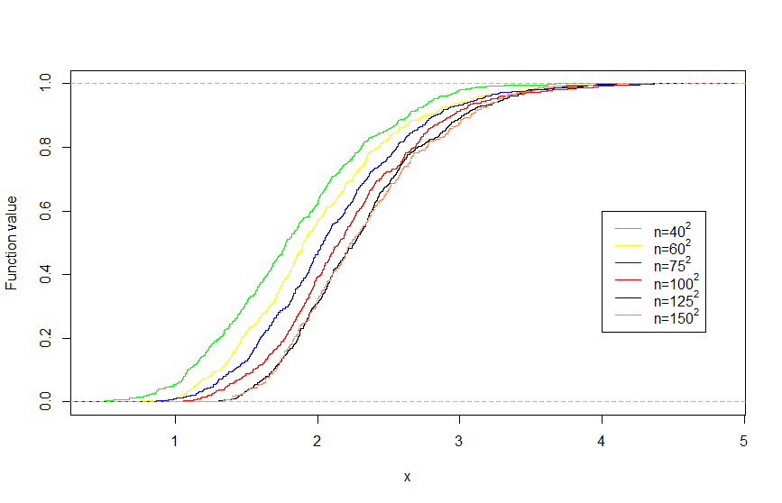
Figure 1: The empirical distribution functions of the multiscale statistic for different values of $n$.

In Tables 2 and 3 we compare the powers of the multiscale test, a test based on a scan-statistic, and the ALR test (see Chan and Walther, [7] for the details). Formally, we consider testing (1.10) against alternatives of the form $H_{1}:f=\mu_{n}\mathbb{I}_{B_{n}}$, for both small and large scale signals ($B_{n}$). We briefly describe the above two competing procedures. Let $\mathscr{B}$ be the set of all axis-aligned rectangles on $[0,1]^{2}$ with corner points of the form $({i}/{m},{j}/{m})$, for $i,j\in\{1,\ldots,m\}$. For every $B\in\mathscr{B}$ define

$$\hat{\Psi}(B):=\frac{1}{\sqrt{|B|}}\sum_{(i/m,j/m)\in B}Y\left(\frac{i}{m},\frac{j}{m}\right).$$

Note that $\hat{\Psi}(\cdot)$ is the discrete analogue of the normalized kernel estimator as defined in (1.6). The scan test statistic (see Glaz et al., [14, Chapter 5]) for this problem is defined as

$$M_{n}:=\max_{B\in\mathscr{B}}|\hat{\Psi}(B)|.$$

The ALR test statistic (see Chan, [6]) is defined as

$$A_{n}:=\frac{1}{{m\choose 2}^{2}}\sum_{B\in\mathscr{B}}\exp(\hat{\Psi}(B)^{2}/2).$$

The scan test (ALR test) rejects the null hypothesis if the observed $M_{n}$ ($A_{n}$) exceeds the 0.95-quantile for $M_{n}$ ($A_{n}$) under the null hypothesis. In Tables 2 and 3 we compare the performance of the three procedures. Here $\mu$ denotes the signal strength, and $k/m$ denotes the length of each side of the square signal $B_{n}$ (here $m=40$ and $100$ for the two cases). The power of the tests were calculated using 1000 replications.

$k=1$
$\mu$	Scan	Multiscale	ALR
3.5	0.23	0.08	0.07
4.0	0.34	0.13	0.08
4.5	0.50	0.18	0.08
5.0	0.71	0.30	0.08
5.5	0.86	0.53	0.09

$k=4$
$\mu$	Scan	Multiscale	ALR
1.00	0.22	0.14	0.11
1.20	0.43	0.31	0.30
1.35	0.60	0.48	0.44
1.50	0.74	0.55	0.52
1.65	0.86	0.72	0.61

$k=18$
$\mu$	Scan	Multiscale	ALR
0.20	0.15	0.21	0.19
0.30	0.49	0.68	0.67
0.35	0.65	0.80	0.82
0.40	0.80	0.90	0.89

$k=40$
$\mu$	Scan	Multiscale	ALR
0.040	0.15	0.32	0.31
0.043	0.30	0.56	0.54
0.047	0.45	0.78	0.78
0.050	0.68	0.94	0.95

Table 2: Power of the scan, the multiscale and the ALR tests for $m=40$ (i.e., $n=40^{2}$) as $\mu$ changes.

We make the following observations. For both the cases ($m=40$ and $100$) when the signal is at the smallest scale, e.g., $k=1$, the scan statistic outperforms everything else. However, when $m=100$, even in relatively small scales, e.g., $k=8$ (i.e., about $0.6\%$ of the observations contain the signal) our multiscale test starts to outperform the scan test. Note that in this setting (small scales) the ALR performs the worst. As the spatial extent of the signal increases, our multiscale procedure and the ALR procedure starts performing favorably whereas the performance of the scan statistics deteriorates. Thus, the simulation experiments corroborates our theoretical findings.

$k=1$
$\mu$	Scan	Multiscale	ALR
4.5	0.34	0.11	0.06
5.0	0.52	0.28	0.06
5.5	0.75	0.43	0.09
6.0	0.95	0.61	0.13

$k=8$
$\mu$	Scan	Multiscale	ALR
0.25	0.08	0.17	0.07
0.30	0.35	0.46	0.13
0.35	0.60	0.72	0.22
0.40	0.82	0.96	0.50

$k=30$
$\mu$	Scan	Multiscale	ALR
0.040	0.07	0.22	0.22
0.050	0.17	0.42	0.45
0.055	0.42	0.74	0.75
0.060	0.58	0.93	0.96

$k=100$
$\mu$	Scan	Multiscale	ALR
0.014	0.08	0.42	0.42
0.018	0.17	0.62	0.63
0.020	0.22	0.84	0.86
0.025	0.45	0.96	0.95

Table 3: Power of the scan, the multiscale and the ALR tests for $m=100$ (i.e., $n=100^{2}$) as $\mu$ changes.

5 Discussion

In this paper we have proposed a multidimensional multiscale statistic in the continuous white noise model and used this statistic to construct asymptotically minimax tests for testing $f=0$ against (i) Hölder classes of functions; and (ii) alternatives of the form $f=\mu_{n}\mathbb{I}_{B_{n}}$, where $B_{n}$ is an unknown axis-aligned hyperrectangle in $[0,1]^{d}$ and $\mu_{n}\in{\mathbb{R}}$ is unknown. However, there are many open questions in this area. We briefly delineate a few of them below and in the process describe some important papers in related areas of research.

We have shown that for the Hölder class $\mathbb{H}_{\beta,L}$, if the smoothness parameter $\beta$ is known, we can construct an asymptotically minimax test. However, if $\beta$ is unknown (and $\beta\leq 1$) we can only construct a rate optimal test. A natural question that arises is whether a test can be constructed that is asymptotically minimax (for the Hölder class of functions with the supremum norm) without the knowledge of the smoothness parameter $\beta$ (and $L>0$); see Ji and Nussbaum, [25, Section 1.3]. Another interesting question would be to try to extend our results to other smoothness classes like Sobolev/Besov classes; in Ingster and Stepanova, [19] the authors gave the minimax rate of testing for Sobolov class, but no test was proposed that achieves the exact separation constant.

Note that we have shown that our multiscale test is asymptotically minimax for detecting the presence of a signal on an axis-aligned hyperrectangle in $[0,1]^{d}$. One obvious extension of our work would be to correctly identify the hyperrectangle on which the signal is present. Further, we could go beyond hyperrectangles and try to identify signals that are present on some other geometric structures $A\subset[0,1]^{d}$ (i.e., $f=\mu\mathbb{I}_{A}$ where $A$ is not necessarily an axis-aligned hyperrectangle). Examples of such geometric structures could be: $(i)$ $A$ is an hyperrectangle which is not necessarily axis-aligned, $(ii)$ $A$ is a $d$-dimensional ellipsoid, $(iii)$ $A=\bigcup_{i=1}^{k}A_{i}$ where each $A_{i}\subseteq[0,1]^{d}$ is an (axis-aligned) hyperrectangle, etc. Frick et al., [12] and the references therein investigated the problem of finding change points in $d=1$ which can be thought of as detection of multiple intervals. In Arias-Castro et al., [3] the authors use the scan statistic to detect regions in $\mathbb{R}^{d}$ where the underlying function is non-zero. Arias-Castro et al., [2] considers the problem of finding a cluster of signals (not necessarily rectangular) in a network using the scan statistic. Although the method they propose achieves the optimal boundary for detection, it requires the knowledge of whether the signal shape is “thick” or “thin”. For hyperrectangles this refers to whether or not the minimum side length is of order $\log n/n$ or not. We believe that the multiscale statistic, with proper modifications, can be used to find asymptotically minimax/rate optimal tests in such problems.

In our white noise model (1.1) we assume that the distribution of the response variables is (homogeneous and independent) Gaussian. Similar questions about signal detection can be asked when the response is non-Gaussian; see e.g., König et al., [28], Chan and Walther, [8], Rivera and Walther, [35], Walther, [42] etc. In Pein et al., [32] the authors looked at the problem of detecting change points under heterogeneous variance of the response variable (when $d=1$). Rohde, [36] looked at this problem where the error distribution is known to be symmetric (when $d=1$). Walther, [42] studied a similar problem where the response variable is binary. A multiscale approach could be used to tackle such problems as well.

Several interesting applications of the multiscale approach exist when $d=1$ (following the seminal paper of Dümbgen and Spokoiny, [10]): In Dümbgen and Walther, [11] the authors propose a multiscale test statistic to make inference about a probability density on the real line given i.i.d. observations; Schmidt-Hieber et al., [37] use multiscale methods to make inference in a deconvolution problem; Rivera and Walther, [35] use multiscale methods to detect a jump in the intensity of a Poisson process, etc. We believe that our extension beyond $d=1$ will also lead to several interesting multidimensional applications.

6 Proofs of our main results

6.1 Some useful concepts

In this subsection we formally define some technical concepts that we use in this paper.

Definition 6.1 (Brownian sheet).

By a $d$-dimensional Brownian sheet we mean a mean-zero Gaussian process $\{W(t):t\in[0,1]^{d}\}$ with covariance

$${\text{Cov}}(W(t_{1},\ldots,t_{d}),W(s_{1},\ldots,s_{d}))=\Pi_{i=1}^{d}\min({t_{i},s_{i}}),$$

for $(t_{1},\ldots,t_{d}),(s_{1},\ldots,s_{d})\in[0,1]^{d}$. The Brownian sheet is the $d$-dimensional counterpart of the standard Brownian motion; see e.g., Wong and Zakai, [44], Khoshnevisan, [27, Chapter 5] for detailed properties of the Brownian sheet.

In the following we give some useful properties of a Brownian sheet $W(\cdot)$.

• If $g\in L_{2}([0,1]^{d})$ then $\int gdW:=\int_{[0,1]^{d}}g(t)dW(t)\sim N(0,\left\lVert g\right\rVert^{2}).$

• If $g_{1},g_{2}\in L_{2}([0,1]^{d})$ then ${\text{Cov}}\left(\int g_{1}dW,\int g_{2}dW\right)=\int_{[0,1]^{d}}g_{1}(t)g_{2}(t)dt.$

• Cameron-Martin-Girsanov Theorem for Brownian sheet: Let us state the simplest version of the Cameron-Martin-Girsanov Theorem that we will use in this paper (see Protter, [34, Chapter 3] for detailed discussion about change of measure and the result).

  Assume $f\in L_{1}([0,1]^{d})$ and let $\{{W(t):t\in[0,1]^{d}}\}$ be a standard Brownian sheet. Let $\Omega$ be the set of all real-valued continuous functions defined on $[0,1]^{d}$. Let $P$ denote the measure on $\Omega$ induced by the Brownian sheet $\{{W(t):t\in[0,1]^{d}}\}$ and let $Q$ denote the measure induced by $\{Y(t):t\in[0,1]^{d}\}$ where $Y(t)$ is defined as in (1.1). Then $Q$ is absolutely continuous with respect to $P$ and the Radon-Nikodym derivative is given by

  $$\frac{dQ}{dP}(Y)=\exp\left(\sqrt{n}\int fdW-\frac{n}{2}\left\lVert f\right\rVert^{2}\right).$$

  This, in turn, implies that for any measurable function $\phi$ we have

  $${\mathbb{E}}_{Q}\left(\phi(Y)\right)={\mathbb{E}}_{P}\left(\phi(Y)\frac{dQ}{dP}(Y)\right).$$

Let us now define the Hölder class of functions $\mathbb{H}_{\beta,L}$, for $\beta>0$ and $L>0$.

Definition 6.2.

Fix $\beta>0$ and $L>0$. Let $\lfloor\beta\rfloor$ be the largest integer which is strictly less than $\beta$ and for $k=(k_{1},k_{2},\ldots,k_{d})\in\mathbb{N}^{d}$ set $\left\lVert k\right\rVert_{1}:=\sum_{i=1}^{d}k_{i}$. The Hölder class $\mathbb{H}_{\beta,L}$ on $[0,1]^{d}$ is the set of all functions $f:[0,1]^{d}\to{\mathbb{R}}$ having all partial derivatives of order $\lfloor\beta\rfloor$ on $[0,1]^{d}$ such that

$$\sum_{0\leq\left\lVert k\right\rVert_{1}\leq\lfloor\beta\rfloor}\sup_{x\in[0,1]^{d}}\left|\frac{\partial^{\left\lVert k\right\rVert_{1}}f(x)}{\partial x_{1}^{k_{1}}\ldots\partial x_{d}^{k_{d}}}\right|\leq L$$

and

$$\sum_{\left\lVert k\right\rVert_{1}=\lfloor\beta\rfloor}\left|\frac{\partial^{\left\lVert k\right\rVert_{1}}f(y)}{\partial x_{1}^{k_{1}}\ldots\partial x_{d}^{k_{d}}}-\frac{\partial^{\left\lVert k\right\rVert_{1}}f(z)}{\partial x_{1}^{k_{1}}\ldots\partial x_{d}^{k_{d}}}\right|\leq L\left\lVert y-z\right\rVert^{\beta-\lfloor\beta\rfloor}\quad\forall\,y,z\in[0,1]^{d}.$$

Remark 6.1.

One of the most important properties of $\mathbb{H}_{\beta,L}$ that we will use is the following: If $f\in\mathbb{H}_{\beta,1}$ then, for any $h=(h_{1},\ldots,h_{d})>0$ and $t\in A_{h}$,

$$g(x_{1},\ldots,x_{d}):=L\min(h)^{\beta}f\left(\frac{x_{1}-t_{1}}{h_{1}},\ldots,\frac{x_{d}-t_{d}}{h_{d}}\right)\in\mathbb{H}_{\beta,L}$$

where $\min(h):=\min_{i=1,\ldots,d}h_{i}$.

Definition 6.3 (Hardy-Krause variation).

The notion of bounded variation for a function $f:{\mathbb{R}}^{d}\to{\mathbb{R}}$, where $d\geq 2$, is more involved than when $d=1$. In fact there is no unique notion of bounded variation for a function when $d\geq 2$. Below we describe the notion of Hardy and Krause variation as given in Aistleitner and Dick, [1], which suffices for our purpose.

Let $f:[-1,1]^{d}\to{\mathbb{R}}$ be a measurable function. Let $a=(a_{1},\ldots,a_{d})$ and $b=(b_{1},\ldots,b_{d})$ be elements of $[-1,1]^{d}$ such that $a<b$ (coordinate-wise). We introduce the d-dimensional difference operator $\Delta^{(d)}$ which assigns to the axis-aligned box $A:=[a,b]$ a d-dimensional quasi-volume

$$\Delta^{(d)}(f;A)=\sum_{j_{1}=0}^{1}\cdots\sum_{j_{d}=0}^{1}(-1)^{j_{1}+\cdots+j_{d}}f(b_{1}+j_{1}(a_{1}-b_{1}),\ldots,b_{d}+j_{d}(a_{d}-b_{d})).$$

Let $m_{1},\ldots,m_{d}\in{\mathbb{N}}$. For $s=1,\ldots,d$, let $-1=:x_{0}^{(s)}<x_{1}^{(s)}<\cdots<x_{m_{s}}^{(s)}:=1$ be a partition of $[-1,1]$ and let $\mathsf{P}$ be a partition of $[-1,1]^{d}$ which is given by

$$\mathsf{P}:=\left\{[x_{l_{1}}^{(1)},x_{l_{1}+1}^{(1)}]\times\cdots\times[x_{l_{d}}^{(d)},x_{l_{d}+1}^{(d)}]:\;l_{s}=0,1,\ldots,m_{s}-1,\;\mbox{for }s=1,\ldots,d\right\}.$$

Then the variation of $f$ on $[-1,1]^{d}$ in the sense of Vitali is given by

$$V^{(d)}(f;[-1,1]^{d}):=\sup_{\mathsf{P}}\sum_{A\in\mathsf{P}}|\Delta^{(d)}(f;A)|$$

where the supremum is extended over all partitions of $[-1,1]^{d}$ into axis-parallel boxes generated by $d$ one-dimensional partitions of $[-1,1]$. For $1\leq s\leq d$ and $1\leq i_{1}<\ldots<i_{s}\leq d$, let $V^{(s)}(f;i_{1},\ldots,i_{s};[-1,1]^{d})$ denote the $s$-dimensional variation in the sense of Vitali of the restriction of $f$ to the face

$$U_{d}^{(i_{1},\ldots,i_{s})}=\left\{(x_{1},\ldots,x_{d})\in[-1,1]^{d}:x_{j}=1\mbox{ for all }j\neq i_{1},\ldots,i_{s}\right\}$$

of $[-1,1]^{d}$. Then the variation of $f$ on $[-1,1]^{d}$ in the sense of Hardy and Krause anchored at 1, abbreviated by HK-variation, is given by

$$TV(f):=\sum_{i=1}^{d}\sum_{1\leq s\leq d}V^{(s)}(f;i_{1},\ldots,i_{s};[-1,1]^{d}).$$

We say a function $f$ has bounded HK-variation if $TV(f)<\infty.$

The main property of a bounded HK-variation function that we will need in this paper is stated below.

Remark 6.2.

If $f$ is a right continuous function on $[-1,1]^{d}$ which has bounded HK-variation then there exists a unique signed Borel measure $\nu$ on $[-1,1]^{d}$ for which

$$f(x)=\nu([-1,x]),\quad x\in[-1,1]^{d};$$

see Aistleitner and Dick, [1] for details.

6.2 Proof of Theorem 2.2

In the following proofs $K$ would be used to denote a generic constant whose value would change from line to line.

For every $v>0$, we define

$$\Gamma(X,v):=\sup_{a,b\in\mathscr{F},\rho(a,b)\leq v}|X(a)-X(b)|.$$

For simplicity we divide the proof in three steps.

Step 1: In this step we will prove that

$${\mathbb{P}}\big{(}\Gamma(X,v)>\eta\big{)}\leq K\exp\left(-\frac{\eta^{2}}{Kv^{2}\log(e/v)}\right)\quad\forall\,\eta>0\mbox{ and }v\in(0,1],$$ (6.1)

where $K>0$ is a positive constant not depending on $v$. We will prove the above result by introducing the notion of Orlicz norm. Let $\lambda:\mathbb{R}_{+}\to\mathbb{R}$ be a nondecreasing convex function with $\lambda(0)=0$. For any random variable $X$ the Orlicz norm $\left\lVert X\right\rVert_{\lambda}$ is defined as

$$\left\lVert X\right\rVert_{\lambda}=\inf\bigg{\{}C>0:{\mathbb{E}}\lambda\left(\frac{|X|}{C}\right)\leq 1\bigg{\}}.$$

The Orlicz norm is of interest to us as any Orlicz norm easily yields a bound on the tail probability of a random variable i.e., ${\mathbb{P}}(|X|>x)\leq[\lambda(x/\left\lVert X\right\rVert_{\lambda})]^{-1},\mbox{ for all }x\in{\mathbb{R}}.$ Let us define $\lambda(x):=\exp(x^{2})-1$, $x>0$. Hence,

$${\mathbb{P}}\big{(}|X|>x\big{)}\leq\min\bigg{\{}1,\frac{1}{\exp(x^{2}/\left\lVert X\right\rVert^{2}_{\lambda})-1}\bigg{\}}\leq 2\times\exp(-x^{2}/\left\lVert X\right\rVert^{2}_{\lambda}).$$ (6.2)

Hence, it is enough to bound the Orlicz norm of $\Gamma(X,v)$. A bound on the Orlicz norm of $\Gamma(X,v)$ can be shown by appealing to van der Vaart and Wellner, [41, Theorem 2.2.4] which we state below.

Lemma 6.1.

Let $\lambda:{\mathbb{R}}_{+}\to{\mathbb{R}}$ be a convex, nondecreasing, non-zero function with $\lambda(0)=0$ and for some constant $c>0$, $\limsup_{x,y\to\infty}\frac{\lambda(x)\lambda(y)}{\lambda(cxy)}<\infty$. Let $\{X_{a},a\in\mathscr{F}\}$ be a separable stochastic process with

$$\left\lVert X_{a}-X_{b}\right\rVert_{\lambda}\leq C\rho(a,b)\mbox{ for all }a,b\in\mathscr{F}$$

for some pseudometric $\rho$ on $\mathscr{F}$ and constant C. Then for any $\zeta,v>0$,

$$\left\lVert\Gamma(X,v)\right\rVert_{\lambda}\leq K\left[\int_{0}^{\zeta}\lambda^{-1}(N(\epsilon,\mathscr{F}))d\epsilon+v\lambda^{-1}(N^{2}(\zeta,\mathscr{F}))\right]$$

for some constant $K$ depending only on $\lambda$ and $C$.

We apply the above lemma with $\lambda(x):=\exp(x^{2})-1$ (i.e., $\lambda^{-1}(y)=\sqrt{\log(1+y)}$). Note that condition (b) of Theorem 2.2 directly implies that $\left\lVert X_{a}-X_{b}\right\rVert_{\lambda}\leq C\rho(a,b)$ by an application of van der Vaart and Wellner, [41, Lemma 2.2.1].

By taking $\delta=1,\epsilon=u^{1/2}$, condition (c) of Theorem 2.2 yields $N(\epsilon,\mathscr{F})\leq A\epsilon^{-2B}$. Thus, Lemma 6.1 gives (with $\zeta=v$)

$$\left\lVert\Gamma(X,v)\right\rVert_{\lambda}\leq K\left[\int_{0}^{v}\sqrt{\log(1+A\epsilon^{-2B})}d\epsilon+v\sqrt{\log(1+A^{2}v^{-4B})}\right].$$

The expression on the right side of the above display can be easily shown to be less than or equal to $Kv\sqrt{\log(e/v)}$ for some constant $K$. This result along with an application of (6.2) with $\Gamma(X,v)$ instead of $X$ imply

$${\mathbb{P}}\big{(}\Gamma(X,v)>\eta\big{)}\leq K\exp\left(-\frac{\eta^{2}}{Kv^{2}\log(e/v)}\right)\qquad\mbox{for all }\eta>0,\;0<v\leq 1,$$

for some constant $K$.

Step 2: Let us define $\mathscr{F(\delta)}:=\{a\in\mathscr{F}:\delta/2<\sigma^{2}(a)\leq\delta\}$, for $\delta\in(0,1]$, and

$$\Pi(\delta):={\mathbb{P}}\left(\frac{X^{2}(a)}{\sigma^{2}(a)}>2V\log(\frac{1}{\delta})+S\log\log(\frac{e^{e}}{\delta})\mbox{ for some }a\in\mathscr{F}(\delta)\right)$$ (6.3)

for $S\geq 4p+1$. In this step we will prove that

$$\Pi(\delta)\leq K\exp((K-S/K)\log\log(e^{e}/\delta))$$

for some constant $K$.

Fix $u<1/2$. Let $\mathscr{F}(\delta,u)$ be a $\sqrt{u\delta}$-packing set of $\mathscr{F(\delta})$. By our assumption the cardinality of $\mathscr{F}(\delta,u)$ is less than or equal to $Au^{-B}\delta^{-V}(\log({e/\delta}))^{p}$. Fix $a\in\mathscr{F}(\delta)$. From the definition of $\mathscr{F}(\delta,u)$ we can associate $\hat{a}\in\mathscr{F}(\delta,u)$ (corresponding to $a\in\mathscr{F}(\delta)$) such that $\rho^{2}(a,\hat{a})\leq u\delta$. Using assumption (a) of Theorem 2.2 we have

$$\sigma^{2}(a)\geq\sigma^{2}(\hat{a})-u\delta\geq\sigma^{2}(\hat{a})(1-2u)$$ (6.4)

where the last inequality follows from the fact that $\hat{a}\in\mathscr{F(\delta})$ (thus $\sigma^{2}(\hat{a})>\delta/2$).

We want to study the event

$$\frac{X^{2}(a)}{\sigma^{2}(a)}>r$$ (6.5)

for some $r>0$. Obviously, for any $\lambda\in(0,1)$, either (i) $|X(a)-X(\hat{a})|^{2}>\lambda^{2}X^{2}(a)$ or (ii) $|X(a)-X(\hat{a})|^{2}\leq\lambda^{2}X^{2}(a)$ (which, in particular implies $|X(\hat{a})|\geq(1-\lambda)|X(a)|$). The above two cases reduce to:

$$\Gamma(X,(u\delta)^{1/2})^{2}\geq|X(a)-X(\hat{a})|^{2}>\lambda^{2}X^{2}(a)\geq\lambda^{2}r\sigma^{2}(a)\geq\lambda^{2}r\frac{\delta}{2}$$ (6.6)

(here the first inequality follows from the definition of $\Gamma(X,(u\delta)^{1/2})$ and the third inequality follows from condition (6.5)), and

$$X^{2}(\hat{a})\geq(1-\lambda)^{2}X^{2}(a)\geq(1-\lambda)^{2}r\sigma^{2}(a)\geq(1-\lambda)^{2}r(1-2u)\sigma^{2}(\hat{a})$$ (6.7)

(here the second inequality follows from (6.5) and last inequality follows from (6.4)). Therefore, for any $r>0$,

$$\Pi_{r}(\delta) := {\mathbb{P}}\left(\frac{X^{2}(a)}{\sigma^{2}(a)}>r\mbox{ for some }a\in\mathscr{F(\delta)}\right)$$

$$\leq {\mathbb{P}}\left(\Gamma(X,(u\delta)^{1/2})^{2}>\lambda^{2}\delta r/2\right)$$

$$\qquad\qquad\qquad+\sum_{\hat{a}\in\mathscr{F}(\delta,u)}{\mathbb{P}}\left(X^{2}(\hat{a})/\sigma^{2}(\hat{a})>(1-\lambda)^{2}r(1-2u)\right)$$

where we have used the fact that if $X^{2}(a)/\sigma^{2}(a)>r$ for some $a\in\mathscr{F}$, then either (6.6) holds or (6.7) is satisfied for some $\hat{a}\in\mathscr{F}(\delta,u)$. The first term on the right side of the above display can be bounded by appealing to (6.1) with $\eta=\sqrt{\lambda^{2}\delta r/2}$ and $v=\sqrt{u\delta}$ and the second term can be bounded by using conditions (a) and (c) of Theorem 2.2. Hence we get

$$\Pi_{r}(\delta) \leq K\exp\left(-\frac{\lambda^{2}\delta r/2}{Ku\delta\log(e/\sqrt{u\delta})}\right)$$

$$\qquad\qquad\qquad+Au^{-B}\delta^{-V}\big{(}\log(\frac{e}{\delta})\big{)}^{p}\exp\left(-\frac{(1-\lambda)^{2}r(1-2u)}{2}\right)$$

$$\leq K\Big{[}\exp\left(-\frac{\lambda^{2}r}{Ku\log(e/(u\delta))}\right)$$

$$\qquad+\exp\big{(}B\log(1/u)+V\log(1/\delta)+p\log\log(e/\delta)+ur-(1/2-\lambda)r\big{)}\Big{]}.$$ (6.8)

Fix $S\geq 8p+1$ and set

$$r:=2V\log(1/\delta)+S\log\log\big{(}\frac{e^{e}}{\delta}\big{)}$$

and

$$\lambda:=\frac{1}{r}\Big{(}(S/4)\log\log(e^{e}/\delta)-p\log\log(e/\delta)\Big{)}.$$

Observe that $r>1$ and $0<\lambda<1/4$. Moreover, we have

$$(1/2-\lambda)r=V\log(1/\delta)+p\log\log(e/\delta)+(S/4)\log\log(e^{e}/\delta).$$

Putting these values in (6.8) gives us

$$\Pi(\delta)\equiv\Pi_{r}(\delta) \leq K\Bigg{[}\exp\left(-\frac{(S-4p)^{2}(\log\log(e^{e}/\delta))^{2}}{Kur\log(e/(u\delta))}\right)$$ (6.9)

$$\quad\quad\quad+\exp\Big{(}B\log(1/u)+ur-(S/4)\log\log(e^{e}/\delta)\Big{)}\Bigg{]}\qquad$$

where we have used the fact that $\lambda^{2}r^{2}=((S/4)\log\log(e^{e}/\delta)-p\log\log(e/\delta))^{2}\geq(S-4p)^{2}(\log\log(e^{e}/\delta))^{2}/16$. Now, let us pick

$$u:=\frac{S}{8r\log(e/\delta)}<\frac{1}{2}.$$

Then we have $\frac{1}{u}\leq K\log^{2}(e/\delta)$ for some constant $K$. Let us consider the two terms on the right side of (6.9) separately. For the first term, using $ur=S[\log(e/\delta)]^{-1}/8$, and that $\frac{1}{u}\leq K\log^{2}(e/\delta)$, we have

$$\frac{(S-4p)^{2}(\log\log(e^{e}/\delta))^{2}}{Kur\log(e/(u\delta))} = \frac{8(S-8p+16p^{2}/S)(\log\log(e^{e}/\delta))^{2}\log(e/\delta)}{K\big{(}\log(e/\delta)+\log(u^{-1})\big{)}}$$

$$\geq (S-8p)(\log\log(e^{e}/\delta))\Big{(}\frac{(\log\log(e^{e}/\delta))\log(e/\delta)}{K\big{(}\log(e/\delta)+\log K+2\log\log(e/\delta)\big{)}}\Big{)}$$

$$\geq (1/K^{\prime})(S-8p)(\log\log(e^{e}/\delta)).$$

Here the last inequality follows from the following fact: As

$$\tau(\delta):=\frac{(\log\log(e^{e}/\delta))\log(e/\delta)}{K\big{(}\log(e/\delta)+\log K+2\log\log(e/\delta)\big{)}}\to\infty,\qquad\mbox{ as }\delta\to 0,$$

we can find a lower bound $K^{\prime}>0$ such that $\tau(\delta)\geq 1/K^{\prime}$ for all $\delta\in(0,1]$.

For the second term on the right side of (6.9) we have

$$B\log(1/u)+ur-(S/4)\log\log(e^{e}/\delta)$$

$$\leq B\log K+2B\log\log(e/\delta)+S/8-(S/4)\log\log(e^{e}/\delta)$$

$$\leq B\log K+2B\log\log(e/\delta)-(S/8)\log\log(e^{e}/\delta)$$

$$\leq B\log K+(2B-S/8)\log\log(e^{e}/\delta).$$

Thus, both the terms on the right side of (6.9) have the form $K\exp[(C-S/K^{\prime})\log\log(e^{e}/\delta)]$ for some constants $K,C,K^{\prime}>0$. Putting these values in (6.9) gives us, for suitable constant $K>0$, we get

$$\Pi(\delta)\leq K\exp\left((K-S/K)\log\log(e^{e}/\delta)\right).$$

Step 3: In this step we will prove that as $S\to\infty$

$${\mathbb{P}}\left(X^{2}(a)/\sigma^{2}(a)>2V\log(1/\sigma^{2}(a))+S\log\log\big{(}\frac{e^{e}}{\sigma^{2}(a)}\big{)}\mbox{ for some }a\in\mathscr{F}\right)\to 0.$$

First let us define

$$\tilde{\Pi}(\delta):={\mathbb{P}}\left(X^{2}(a)/\sigma^{2}(a)>2V\log(1/\sigma^{2}(a))+S\log\log\big{(}\frac{e^{e}}{\sigma^{2}(a)}\big{)}\mbox{ for some }a\in\mathscr{F}(\delta)\right).$$

Comparing with (6.3) we can see that for any $\delta\in(0,1]$,

$$\tilde{\Pi}(\delta)\leq\Pi(\delta)$$

as: If $a\in\mathscr{F}(\delta)$ then $\sigma^{2}(a)\leq\delta$ and $x\longmapsto 2V\log(1/x)+S\log\log(e^{e}/x)$ is a decreasing function of $x$. Hence, we have

$$\tilde{\Pi}(\delta)\leq K\exp\left((K-S/K)\log\log(e^{e}/\delta)\right).$$

Therefor, as $\mathscr{F}=\bigcup_{l\geq 0}\mathscr{F}(2^{-l})$,

$${\mathbb{P}}\Big{(}X^{2}(a)/\sigma^{2}(a) >2V\log(1/\sigma^{2}(a))+S\log\log(\frac{e^{e}}{\sigma^{2}(a)})\mbox{ for some }a\in\mathscr{F}\Big{)}$$

$$\leq\sum_{l=0}^{\infty}\tilde{\Pi}(2^{-l})$$

$$\leq K\sum_{l=0}^{\infty}\exp((K-S/K)\log\log(e^{e}2^{l}))$$

$$=K\sum_{l=0}^{\infty}(e+l\log 2)^{-(S/K-K)}\quad\to 0\quad\mbox{ as }S\to\infty.$$

This proves that $S(X):=\sup_{a\in\mathscr{F}}\frac{X^{2}(a)/\sigma^{2}(a)-2V\log(1/\sigma^{2}(a))}{\log\log(e^{e}/\sigma^{2}(a))}<\infty$ a.s.∎

6.3 Proof of Lemma 2.1

First let us define the following sets:

$$\mathscr{F}_{\delta,(l_{1},\ldots,l_{d})} := \big{\{}(t,h)\in\mathscr{F}:\delta/2<\sigma^{2}(t,h)\leq\delta,\;2^{l_{i}-1}<\frac{h_{i}}{\delta^{1/d}}\leq 2^{l_{i}},\;\forall\;i=1,\ldots,d\big{\}}$$

$$\hskip 180.67499pt\mbox{ for some }(l_{1},\ldots,l_{d})\in\mathbb{Z}^{d},$$

$$\mathscr{F}(\delta) := \big{\{}(t,h)\in\mathscr{F}:\delta/2<\sigma^{2}(t,h)\leq\delta\big{\}}.$$

We note that $\mathscr{F}_{\delta,(l_{1},\ldots,l_{d})}$ is empty unless we have

$$\mathrm{(i)}\quad l_{i}\leq(1/d)\log_{2}(1/\delta)\qquad\mbox{for all }i=1,\ldots,d;$$

(this restriction is a consequence of the fact that $h_{i}\leq 1/2$) and

$$\mathrm{(ii)}\quad-(d+1)<\sum_{i=1}^{d}l_{i}\leq 0$$

(this restriction is a consequence of the fact that $\delta/2<\sigma^{2}(t,h)\leq\delta$).

Step 1: First, we will show that for any $(l_{1},\ldots,l_{d})\in\mathbb{Z}^{d}$, and $\delta,u\in(0,1]$,

$$N\left((u\delta)^{1/2},\mathscr{F}_{\delta,(l_{1},\ldots,l_{d})}\right)\leq Ku^{-2d}\delta^{-1}.$$ (6.10)

Let $\mathscr{F}^{\prime}$ be a subset of $\mathscr{F}_{\delta,(l_{1},\ldots,l_{d})}$ such that for any two elements $(t,h),(t^{\prime},h^{\prime})\in\mathscr{F}^{\prime}$ we have

$$\rho^{2}((t,h),(t^{\prime},h^{\prime}))>u\delta.$$ (6.11)

Our aim is to show that

$$|\mathscr{F}^{\prime}|\leq Ku^{-2d}\delta^{-1},$$

for some constant $K$ independent of $(l_{1},\ldots,l_{d})$, $u$ and $\delta$. If $\mathscr{F}_{\delta,(l_{1},\cdots,l_{d})}$ is empty then the assertion is trivial. So assume that $\mathscr{F}_{\delta,(l_{1},\cdots,l_{d})}$ is non-empty which imposes bounds on the $l_{i}$’s as shown above.

Let us define the following partition of $[0,1]^{d}$ into disjoint hyperrectangles:

$$R:=\Big{\{}M_{(i_{1},\ldots,i_{d})}\cap[0,1]^{d}:M_{(i_{1},\ldots,i_{d})}:=\Pi_{k=1}^{d}\Big{(}(i_{k}-1)\frac{u\delta^{\frac{1}{d}}2^{l_{k}}}{c},i_{k}\frac{u\delta^{\frac{1}{d}}2^{l_{k}}}{c}\Big{]},$$

$$\qquad\qquad\>1\leq i_{k}\leq\lceil cu^{-1}\delta^{-\frac{1}{d}}2^{-l_{k}}\rceil\Big{\}}$$

where we take $c:=d4^{d}$. We would like to point out that in the above definition when $i_{k}=1$, for any $k=1,\ldots,d$, by $\big{(}(i_{k}-1)c^{-1}u\delta^{1/d}2^{l_{k}},$ $i_{k}c^{-1}u\delta^{1/d}2^{l_{k}}\big{]}$ we mean the closed interval $\big{[}0,c^{-1}u\delta^{1/d}2^{l_{k}}\big{]}$. Observe that all the sets in $R$ are disjoint and moreover

$$\bigcup_{M\in R}M=[0,1]^{d}.$$

Observe that

$$2^{l_{i}-1}\delta^{1/d}<h_{i}\leq 1/2\;\;\Rightarrow\;\;2^{l_{i}}\delta^{1/d}<1 \Rightarrow cu^{-1}\delta^{-1/d}2^{-l_{i}}>1$$

$$\Rightarrow \lceil cu^{-1}\delta^{-1/d}2^{-l_{i}}\rceil\leq 2cu^{-1}\delta^{-1/d}2^{-l_{i}}.$$

Hence we can easily see that

$$|R|=\Pi_{i=1}^{d}\lceil cu^{-1}\delta^{-1/d}2^{-l_{i}}\rceil\leq 2^{d}c^{d}u^{-d}\delta^{-1}2^{-\sum_{i=1}^{d}l_{i}}\leq 2^{2d+1}c^{d}u^{-d}\delta^{-1}.$$

Here the last inequality follows from the fact that $\sum_{i=1}^{d}l_{i}\geq-(d+1)$.

Let us define the following set:

$$R_{2}:=\Big{\{}(M_{\underset{\sim}{i}},M_{\underset{\sim}{i}^{\prime}})\in R\times R:\exists\;(t,h)\in\mathscr{F}^{\prime}\mbox{ such that }t-h\in M_{\underset{\sim}{i}}\mbox{ and }t+h\in M_{\underset{\sim}{i}^{\prime}}\Big{\}}.$$

Note that if $(t,h)\in\mathscr{F}^{\prime}$ then $h_{k}\leq 2^{l_{k}}\delta^{1/d}$ for all $k=1,\ldots,d$. This implies that if $(M_{\underset{\sim}{i}},M_{\underset{\sim}{i}^{\prime}})\in R_{2}$, where $\underset{\sim}{i}=(i_{1},\ldots,i_{d})$ and $\underset{\sim}{i}^{\prime}=(i^{\prime}_{1},\ldots,i^{\prime}_{d})$, then

$$(i^{\prime}_{k}-i_{k})\leq(1+2cu^{-1}),\qquad\mbox{ for all }\;k=1,\ldots,d,$$ (6.12)

as (i) $(i^{\prime}_{k}-1)u\delta^{{1}/{d}}2^{l_{k}}c^{-1}\leq t_{k}+h_{k}$, and (ii) $i_{k}u\delta^{\frac{1}{d}}2^{l_{k}}c^{-1}\geq t_{k}-h_{k}$. Thus for each hyperrectangle $M_{\underset{\sim}{i}}\in R$ the number of hyperrectangles $M_{\underset{\sim}{i}^{\prime}}\in R$ such that $(M_{\underset{\sim}{i}},M_{\underset{\sim}{i}^{\prime}})\in R_{2}$ is less than or equal to $(1+2cu^{-1})^{d}\leq 4^{d}c^{d}u^{-d}$. Hence we have

$$|R_{2}|\leq|R|\times 4^{d}c^{d}u^{-d}\leq 2^{4d+1}c^{2d}u^{-2d}\delta^{-1}\leq d^{2d}2^{4d^{2}+4d+1}u^{-2d}\delta^{-1}.$$

Thus, our proof will be complete if we can show that $|R_{2}|=|\mathscr{F}^{\prime}|$. From the definition of $R_{2}$ and the fact that elements in $R$ are disjoint it is easy to observe that $|R_{2}|\leq|\mathscr{F}^{\prime}|$.

Therefore, the only thing left to show is that $|\mathscr{F}^{\prime}|\leq|R_{2}|$. Let us assume the contrary, i.e., $|R_{2}|<|\mathscr{F}^{\prime}|$. This implies that there exist two elements $(t,h)$ and $(t^{\prime},h^{\prime})\in\mathscr{F}^{\prime}$ and $(M_{\underset{\sim}{i}},M_{\underset{\sim}{i}^{\prime}})\in R_{2}$ such that both $t-h$ and $t^{\prime}-h^{\prime}$ belong to $M_{\underset{\sim}{i}}$ and, also, $t+h$ and $t^{\prime}+h^{\prime}$ belong to $M_{\underset{\sim}{i}^{\prime}}$. Let us first define the following two hyperrectangles:

$$B_{1}:=\Pi_{k=1}^{d}(i_{k}-1,i^{\prime}_{k}]\times c^{-1}u\delta^{1/d}2^{l_{k}}\qquad\mbox{ and }\qquad B_{2}:=\Pi_{k=1}^{d}(i_{k},i^{\prime}_{k}-1]\times c^{-1}u\delta^{1/d}2^{l_{k}}.$$

Our goal is to show that

$$B_{\infty}(t,h)\bigtriangleup B_{\infty}(t^{\prime},h^{\prime})\subseteq B_{1}\setminus B_{2}$$ (6.13)

which is implied by the following two assertions:

1. $B_{\infty}(t,h)\cup B_{\infty}(t^{\prime},h^{\prime})\subseteq B_{1}$ and

2. $B_{2}\subseteq B_{\infty}(t,h)\cap B_{\infty}(t^{\prime},h^{\prime})$.

See the figure below for a visual illustration of (6.13) when $d=2$.

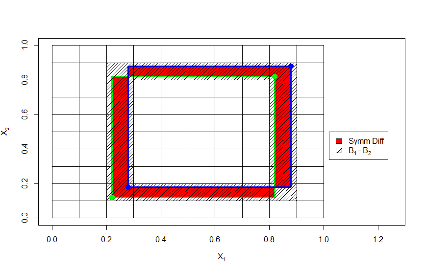
Figure 2: The figure shows how the symmetric difference of the hyperrectangles $B_{\infty}(t,h)$ (denoted by the green border) and $B_{\infty}(t^{\prime},h^{\prime})$ (denoted by the blue border) is contained in the set $B_{1}\setminus B_{2}$ (denoted by the shaded region).

Now, as $t-h\in M_{\underset{\sim}{i}}$, this implies $t_{k}-h_{k}\geq(i_{k}-1)c^{-1}u\delta^{1/d}2^{l_{k}}$, for all $k=1,\ldots,d$. Also $t+h\in M_{\underset{\sim}{i}^{\prime}}$ implies that $t_{k}+h_{k}\leq i^{\prime}_{k}c^{-1}u\delta^{1/d}2^{l_{k}}$, for all $k=1,\ldots,d.$ Therefore, $B_{\infty}(t,h)=\Pi_{i=1}^{d}(t_{i}-h_{i},t_{i}+h_{i})\subseteq B_{1}$. A similar argument shows that $B_{\infty}(t^{\prime},h^{\prime})\subseteq B_{1}$. Hence assertion $(1)$ above holds.

Now as $t-h\in M_{\underset{\sim}{i}}$, we have $t_{k}-h_{k}\leq i_{k}c^{-1}u\delta^{1/d}2^{l_{k}}$, for all $k=1,\ldots,d.$ Also $t+h\in M_{\underset{\sim}{i}^{\prime}}$ implies that $t_{k}+h_{k}\geq(i^{\prime}_{k}-1)c^{-1}u\delta^{1/d}2^{l_{k}}$, for all $k=1,\ldots,d$. Hence we have $B_{2}\subseteq B_{\infty}(t,h)$. A similar argument shows that $B_{2}\subseteq B_{\infty}(t^{\prime},h^{\prime})$. Therefore, assertion $(2)$ is also satisfied. Now let us define the following set

$$I:=\big{\{}{\underset{\sim}{j}}=(j_{1},\ldots,j_{d})\in\mathbb{N}^{d} : j_{k}\in(i_{k}-1,i^{\prime}_{k}],\mbox{ for all }k=1,\ldots,d,$$

$$\exists\>l\in\{1,\ldots,d\}\mbox{ such that }j_{l}=i_{l}\mbox{ or }i_{l}^{\prime}\big{\}}.$$

Clearly, using (6.12),

$$|I|\leq 2d(2+2cu^{-1})^{d-1}.$$

Also see that $w=(w_{1},\ldots,w_{d})\in B_{1}\setminus B_{2}$ if and only if

1. for every $k=1,\ldots,d$, we have $w_{k}\in\big{(}i_{k}-1,i_{k}^{\prime}\big{]}\times c^{-1}u\delta^{1/d}2^{l_{k}}$ (this is true as $w\in B_{1}$),

2. there exists $l\in\{1,2,\ldots,d\}$ such that either $w_{l}\in\big{(}i_{l}-1,i_{l}\big{]}\times c^{-1}u\delta^{1/d}2^{l_{l}}$ or $w_{l}\in\big{(}i_{l}^{\prime}-1,i_{l}^{\prime}\big{]}\times c^{-1}u\delta^{1/d}2^{l_{l}}$ (this is true as $w\not\in B_{2}$ implies that there exist $l$ such that $w_{l}\not\in(i_{l},i_{l}^{\prime}-1]\times c^{-1}u\delta^{1/d}2^{l_{l}}$ and $w\in B_{1}$ implies that $w_{l}\in(i_{l}-1,i_{l}^{\prime}]\times c^{-1}u\delta^{1/d}2^{l_{l}}$).

Therefore, we see that

$$B_{1}\setminus B_{2}=\bigcup_{{\underset{\sim}{j}}\in I}M_{{\underset{\sim}{j}}}.$$

Also, note that, $|M_{\underset{\sim}{j}}|\leq u^{d}\delta c^{-d}2^{\sum_{i=1}^{d}l_{i}}\leq u^{d}\delta c^{-d}$ for all ${\underset{\sim}{j}}$. Therefore, using (6.13) and the fact that $c=d4^{d}$, we easily see that

$$\rho^{2}((t,h),(t^{\prime},h^{\prime}))\leq|B_{1}\setminus B_{2}|\leq 2d(2+2cu^{-1})^{d-1}\times\frac{u^{d}\delta}{c^{d}}\leq 2^{d}d(1+c^{-1})^{d-1}u\delta c^{-1}<u\delta$$

which contradicts (6.11). This proves that two elements of $\mathscr{F}^{\prime}$ cannot correspond to the same pair of hyperrectangles $(M_{\underset{\sim}{i}},M_{\underset{\sim}{i}^{\prime}})\in R_{2}$. Hence we have proved (6.10).

Step 2: In this part of the proof we show that

$$N\left((u\delta)^{1/2},\mathscr{F}(\delta)\right)\leq Ku^{-2d}\delta^{-1}(\log(e/\delta))^{d-1}.$$ (6.14)

Let us define the set

$$S:=\Big{\{}(l_{1},\ldots,\l_{d})\in\mathbb{Z}^{d}:-(d+1)<\sum_{k=1}^{d}l_{k}\leq 0\mbox{ and }l_{k}\leq\frac{1}{d}\log_{2}(1/\delta)\mbox{ for all }k=1,\ldots,d\Big{\}}.$$

Now it can be easily seen that $l:=(l_{1},\cdots,\l_{d})\in S$ implies $l_{k}\geq-(d+1)-(d-1)(1/d)\log_{2}(1/\delta)$, for all $k=1,\ldots,d$. This shows that each $l_{k}$ can only take at most $(d+2)+\log_{2}(1/\delta)\leq(d+2)+\log(1/\delta)\log_{2}(e)\leq d+2(\log(e/\delta))$ many values. This shows that

$$|S|\leq(d+1)(d+2\log(e/\delta))^{d-1}\leq(d+2)^{d}(\log(e/\delta))^{d-1}.$$

Note that the power of $(d+2\log(e/\delta))$ in the above display is $d-1$ because if we fix the values of $l_{1},l_{2},\ldots,l_{d-1}$ then $l_{d}$ can only take at most $(d+1)$ values such that $(l_{1},l_{2},\ldots l_{d})\in S$ (as $\sum_{k=1}^{d}l_{k}$ can take at most $d+1$ distinct values). Also note that

$$\mathscr{F}(\delta)\subseteq\bigcup_{l\in S}\mathscr{F}_{\delta,l}.$$

The above representation of $\mathscr{F}(\delta)$ along with the trivial fact that $N(\epsilon,\bigcup_{i=1}^{n}A_{i})\leq\sum_{i=1}^{n}N(\epsilon,A_{i})$ gives us (6.14).
Step 3: In this step we will complete the proof of Lemma 2.1. We want control the $\sqrt{u\delta}$-packing number of the set $\{(t,h)\in\mathscr{F}:\sigma^{2}(t,h)\leq\delta\}$ which can be decomposed in the following way: for $u\in(0,1]$,

$$\{(t,h)\in\mathscr{F}:\sigma^{2}(t,h)\leq\delta\}=\left(\bigcup_{l=0}^{\lfloor 1+\log_{2}(1/u)\rfloor}\mathscr{F}(\delta 2^{-l})\right)\cup\{a\in\mathscr{F}:\sigma^{2}(a)\leq u\delta/2\}.$$

Now we can control the $\sqrt{u\delta}$-packing number of each of the above sets. First observe that

$$N((u\delta)^{1/2},\{(t,h)\in\mathscr{F}:\sigma^{2}(t,h)\leq u\delta/2\})=1.$$

Also, for any $u\in(0,2)$ and $\delta\in(0,1]$ we have

$$N((u\delta)^{1/2},\mathscr{F}(\delta))\leq N((u\delta/2)^{1/2},\mathscr{F}(\delta))\leq Ku^{-2d}\delta^{-1}(\log(e/\delta))^{d-1}$$ (6.15)

for some constant $K$. Putting $\delta\leftarrow\delta/2^{l}$ and $u\leftarrow 2^{l}u$ for $0\leq l\leq\lfloor 1+\log_{2}(1/u)\rfloor$ in (6.15) we get

$$N((u\delta)^{1/2},\mathscr{F}(\delta 2^{-l}))\leq K2^{-(2d-1)l}u^{-2d}\delta^{-1}(\log(e/\delta))^{d-1}.$$

Now from the trivial fact that $N(\epsilon,\bigcup_{i=1}^{m}A_{i})\leq\sum_{i=1}^{m}N(\epsilon,A_{i})$ we get

$$N\left(\sqrt{u\delta},\{(t,h)\in\mathscr{F}:\sigma^{2}(t,h)\leq\delta\}\right)$$

$$\leq \sum_{l=0}^{\lfloor 1+\log_{2}(1/u)\rfloor}N\left(\sqrt{u\delta},\mathscr{F}(\delta 2^{-l})\right)+N\left(\sqrt{u\delta},\{(t,h)\in\mathscr{F}:\sigma^{2}(t,h)\leq u\delta/2\}\right)$$

$$\leq 1+Ku^{-2d}\delta^{-1}(\log(e/\delta))^{d-1}\sum_{l=0}^{\infty}2^{-(2d-1)l}$$

$$\leq 1+2Ku^{-2d}\delta^{-1}(\log(e/\delta))^{d-1}$$

$$\leq (2K+1)u^{-2d}\delta^{-1}(\log(e/\delta))^{d-1},$$

which proves Lemma 2.1. ∎

6.4 Proof of Theorem 2.1

We use Theorem 2.2 to prove Theorem 2.1. Let us recall the definitions of $\mathscr{F},\sigma$ and $\rho$ as introduced just before Lemma 2.1. Without loss of generality we assume that $\left\lVert\psi\right\rVert=1$. For $h\in(0,1/2]^{d}$, let us define the stochastic process

$$X(t,h):=2^{d/2}(h_{1}h_{2}\ldots h_{d})^{1/2}\hat{\Psi}(t,h)=2^{d/2}\int\psi_{t,h}(x)dW(x),\qquad t\in A_{h},$$

where $W(\cdot)$ is the standard Brownian sheet on $[0,1]^{d}$. This defines a centered Gaussian process with $\mathrm{Var}\big{(}X(t,h)\big{)}=\sigma^{2}(t,h)$. Also by a standard calculation on the variance we have $\mathrm{Var}\big{(}X(t,h)-X(t^{\prime},h^{\prime})\big{)}\leq 2^{d}TV^{2}(\psi)\rho^{2}((t,h),(t^{\prime},h^{\prime}))$. As $X(t,h)$ and $X(t,h)-X(t^{\prime},h^{\prime})$ have normal distributions this shows that conditions (a) and (b) of Theorem 2.2 are satisfied. Condition (c) is also satisfied because of Lemma 2.1. Thus, by an application of Theorem 2.2 we have

$$\sup_{0<h\leq 1/2}\sup_{t\in A_{h}}\frac{\hat{\Psi}^{2}(t,h)-2\log(1/2^{d}h_{1}h_{2}...h_{d})}{\log\log(e^{e}/2^{d}h_{1}h_{2}...h_{d})}<\infty.$$

For notational simplicity, let us define $\kappa_{1}:=2\log(1/\sigma^{2}(t,h))$ and $\kappa_{2}:=2\sqrt{2}S\log\log({e^{e}/\sigma^{2}(t,h)})$. Therefore,

$${\small{\mathbb{P}}\left(|\hat{\Psi}(t,h)|\leq\sqrt{2\log\left(\frac{1}{\sigma^{2}(t,h)}\right)}+S\Bigg{(}\frac{\log\log(e^{e}/\sigma^{2}(t,h))}{\log^{\frac{1}{2}}(1/\sigma^{2}(t,h))}\Bigg{)}\;\;\forall\;(t,h)\in\mathscr{F}\right)}$$

$$= {\mathbb{P}}\left(|\hat{\Psi}(t,h)|\leq\kappa_{1}^{1/2}+\kappa_{1}^{-1/2}\kappa_{2}/2\quad\forall\;(t,h)\in\mathscr{F}\right)$$

$$= {\mathbb{P}}\left(\hat{\Psi}(t,h)^{2}\leq\Big{(}\kappa_{1}^{1/2}+\kappa_{1}^{-1/2}\kappa_{2}/2\Big{)}^{2}\>\forall(t,h)\in\mathscr{F}\right)$$

$$\geq {\mathbb{P}}\left(\hat{\Psi}(t,h)^{2}\leq\kappa_{1}+\kappa_{2}\quad\forall(t,h)\in\mathscr{F}\right)$$

$$= {\mathbb{P}}\left(\sup_{t,h\in\mathscr{F}}\frac{\hat{\Psi}^{2}(t,h)-2\log(1/2^{d}h_{1}h_{2}...h_{d})}{\log\log(e^{e}/2^{d}h_{1}h_{2}...h_{d})}<2\sqrt{2}S\right)\;\to\;1\quad\mbox{ as }S\to\infty.\qed$$

Appendix A Proofs of other results

A.1 Proof of Proposition 2.1

The proof of this result follows from the following result. Suppose that $Z_{1},Z_{2},\ldots,Z_{n}$ are i.i.d. standard normal random variables. Then, we know that

$$\frac{\max_{1\leq i\leq n}Z_{i}}{\sqrt{2\log n}}\rightarrow 1\quad\mbox{ a.s}.$$

Let $F_{n}$ be the distribution function of $\max_{1\leq i\leq n}Z_{i}/\sqrt{2\log n}$, i.e., $F_{n}(x):={\mathbb{P}}({\max_{1\leq i\leq n}Z_{i}}\leq x\sqrt{2\log n})$, for $x\in{\mathbb{R}}$. Therefore, for every $x<1$, we have $F_{n}(x)\to 0.$ We want to show that

$$\sup_{(t,h)\in\mathscr{F}}|\hat{\Psi}(t,h)|-\Gamma_{V}(2^{d}h_{1}\ldots h_{d})=\infty\quad\mbox{a.s.}$$

Hence it is enough to show that for every $s\in{\mathbb{R}}$ we have ${\mathbb{P}}(\sup_{(t,h)\in\mathscr{F}}|\hat{\Psi}(t,h)|-\Gamma_{V}(2^{d}h_{1}\ldots h_{d})<s)=0$. Fix $m\in{\mathbb{N}}$. Now,

$${\mathbb{P}}\left(\sup_{(t,h)\in\mathscr{F}}|\hat{\Psi}(t,h)|-\Gamma_{V}(2^{d}h_{1}\ldots h_{d})<s\right)$$

$$\leq {\mathbb{P}}\left(\sup_{t\in A_{\left(\frac{1}{2m},\ldots,\frac{1}{2m}\right)}}\left|\hat{\Psi}\left(t,\left(\frac{1}{2m},\ldots,\frac{1}{2m}\right)\right)\right|-\Gamma_{V}(m^{-d})<s\right)$$

$$\leq {\mathbb{P}}\left(\sup_{t\in A_{m}^{\star}}|\hat{\Psi}(t,({2m})^{-1})|-\Gamma_{V}(m^{-d})<s\right)$$

where $A_{m}^{\star}:=\{(t_{1},\ldots,t_{d}):t_{i}=k_{i}/2m\mbox{ for some odd integer }k_{i}<2m,\;\mbox{for all }\;i=1,\ldots,d\}$. Thus, the last term in the above display can be further upper bounded by

$${\mathbb{P}}\left(\sup_{t\in A_{m}^{\star}}\frac{\hat{\Psi}(t,(2m)^{-1})}{\sqrt{2\log(m^{d})}}-\sqrt{V}<\frac{s}{\sqrt{2\log(m^{d})}}\right)=F_{m^{d}}(\sqrt{V}+s/\sqrt{2\log(m^{d})}),$$

where we have used the fact that now we are dealing with $m^{d}$ i.i.d. standard normal random variables. Now, for every $s>0$, choose $m$ such that $\sqrt{V}+s/\sqrt{2\log(m^{d})}<1-\epsilon$, for some fixed $\epsilon>0$. Hence, $F_{m^{d}}(\sqrt{V}+s/\sqrt{2\log(m^{d})})\leq F_{m^{d}}(1-\epsilon)$, if $m$ is large enough. As this is true for all large $m$, taking $m\to\infty$ gives us the desired result. ∎

A.2 Solution to (3.1)

Let $\psi\in\mathbb{H}_{\beta,1}$ such that $\psi(0)\geq 1.$ Hence by the property of $\mathbb{H}_{\beta,1}$ we have

$$|\psi(x)-\psi(0)|\leq\left\lVert x\right\rVert^{\beta},\qquad\mbox{for all }x\in{\mathbb{R}}^{d},$$

which implies $\psi(x)\geq 1-\left\lVert x\right\rVert^{\beta}$. Hence, on the set $\left\lVert x\right\rVert\leq 1$, we have $\psi(x)\geq 1-\left\lVert x\right\rVert^{\beta}\geq 0.$ Therefore, we have

$$\int_{\left\lVert x\right\rVert\leq 1}\psi^{2}(x)dx\geq\int_{\left\lVert x\right\rVert\leq 1}(1-\left\lVert x\right\rVert^{\beta})^{2}dx\quad\Rightarrow\quad\left\lVert\psi\right\rVert\geq\left\lVert\psi_{\beta}\right\rVert,$$

where $\psi_{\beta}(x)=(1-\left\lVert x\right\rVert^{\beta})\mathbb{I}({\left\lVert x\right\rVert\leq 1}).$ Hence the only thing left to prove is that $\psi_{\beta}\in\mathbb{H}_{\beta,1}$. Suppose that $x,y\in\mathbb{R}^{d}$ such that $1\geq\left\lVert x\right\rVert\geq\left\lVert y\right\rVert$. Then

$$\begin{split}0\leq\psi_{\beta}(y)-\psi_{\beta}(x)=\left\lVert x\right\rVert^{\beta}-\left\lVert y\right\rVert^{\beta}\leq(\left\lVert x\right\rVert-\left\lVert y\right\rVert)^{\beta}\leq\left\lVert x-y\right\rVert^{\beta}.\end{split}$$

Here the the third inequality follows from the fact that when $\beta\leq 1$ the function $u\mapsto u^{\beta}$ is a $\beta$-Hölder continuous function; the last inequality follows from the triangle inequality. If $x,y\in\mathbb{R}^{d}$ such that $\left\lVert x\right\rVert\geq 1\geq\left\lVert y\right\rVert$ then we have

$$\begin{split}0\leq\psi_{\beta}(y)-\psi_{\beta}(x)=1-\left\lVert y\right\rVert^{\beta}\leq(1-\left\lVert y\right\rVert)^{\beta}\leq(\left\lVert x\right\rVert-\left\lVert y\right\rVert)^{\beta}\leq\left\lVert x-y\right\rVert^{\beta}.\end{split}$$

If $x,y\in{\mathbb{R}}^{d}$ is such that $\left\lVert x\right\rVert\geq\left\lVert y\right\rVert\geq 1$ then the assertion is trivial. Hence we have proved that $\psi_{\beta}$ minimizes (3.1). ∎

A.3 Proofs of Theorems 3.1 and 3.2

The proofs of Theorems 3.1 and 3.2 depend on the following lemma (stated and proved in Dümbgen and Spokoiny, [10, Lemma 6.2]).

Lemma A.1.

Let $Z_{1},Z_{2},\ldots$ be a sequence of independent standard normal variables. If $w_{m}:=(1-\epsilon_{m})\sqrt{2\log m}$ with $\lim_{m\to\infty}\epsilon_{m}=0$ and $\lim_{m\to\infty}\epsilon_{m}\sqrt{\log m}=\infty$, then we have

$$\lim_{m\to\infty}{\mathbb{E}}\left|\frac{1}{m}\sum_{i=1}^{m}\exp\left(w_{m}Z_{i}-\frac{w_{m}^{2}}{2}\right)-1\right|=0.$$

A.3.1 Proof of Theorem 3.1

Proof of part (a). For any bandwidth $h=(h_{1},\ldots,h_{d})\in(0,1/2]^{d}$ and $t=(t_{1},\ldots,t_{d})\in A_{h}$, let us define the function $g_{t}:[0,1]^{d}\to{\mathbb{R}}$ as

$$g_{t}(x):=L\min(h)^{\beta}\psi^{(\beta)}_{t,h}(x),\quad\mbox{for }x\in[0,1]^{d},$$

where $\min(h):=\min\{h_{1},h_{2},\ldots,h_{d}\}$ and $\psi_{t,h}^{(\beta)}(x_{1},\ldots,x_{d})=\psi_{\beta}((x_{1}-t_{1})/h_{1},\ldots,(x_{d}-t_{d})/h_{d})$. Elementary calculations show that $g_{t}\in\mathbb{H}_{\beta,L}$ and $\|g_{t}\|_{\infty}=L\min(h)^{\beta}$. Now let us define the set

$$S:=\big{\{}t\in A_{h}:t_{i}=k_{i}h_{i}\mbox{ for some odd integer }k_{i},i=1,\ldots,d\big{\}}.$$

Let $\phi_{n}$ be an arbitrary test for (1.2) with level $\alpha$. Then,

$$\inf_{g\in\mathbb{H}_{\beta,L}:\left\lVert g\right\rVert_{\infty}=L\min(h)^{\beta}}{\mathbb{E}}_{g}[\phi_{n}{(Y)}]-\alpha \;\leq\min_{g_{t}:t\in S}{\mathbb{E}}_{g_{t}}[\phi_{n}(Y)]-{\mathbb{E}}_{0}[\phi_{n}(Y)]$$ (A.1)

$$\leq\;|S|^{-1}\sum_{t\in S}{\mathbb{E}}_{g_{t}}[\phi_{n}(Y)]-{\mathbb{E}}_{0}[\phi_{n}(Y)]$$

$$\leq\;{\mathbb{E}}_{0}\Bigg{[}\Big{(}|S|^{-1}\sum_{t\in S}\frac{dP_{g_{t}}}{dP_{0}}(Y)-1\Big{)}\phi_{n}(Y)\Bigg{]}$$

$$\leq\;{\mathbb{E}}_{0}\Big{|}|S|^{-1}\sum_{t\in S}\frac{dP_{g_{t}}}{dP_{0}}(Y)-1\Big{|}.$$

Here $P_{0}$ denotes the measure of the process $Y$ under the null hypothesis $f=0$ and $P_{g_{t}}$ denotes the measure of $Y$ under the alternative $f=g_{t}$. Also for $g\in\mathbb{H}_{\beta,L}$, $\frac{dP_{g}}{dP_{0}}$ denotes the Radon-Nikodym derivative of the measure $P_{g}$ with respect to the measure $P_{0}$. By Cameron-Martin-Girsanov’s Theorem (see Protter, [34, Chapter 3] for more details about absolute continuous measures and Radon-Nikodym derivatives) we get that

$$\log\left(\frac{dP_{g}}{dP_{0}}(Y)\right)=\sqrt{n}\int gdW-\frac{n}{2}\left\lVert g\right\rVert^{2}.$$

For $g_{t}(\cdot)=L\min(h)^{\beta}\psi^{(\beta)}_{t,h}(\cdot)$, $\sqrt{n}\int g_{t}dW=\sqrt{n}L\left\lVert\psi_{\beta}\right\rVert\min(h)^{\beta}\sqrt{\Pi_{i=1}^{d}h_{i}}\hat{\Psi}(t,h).$ Observe that $\{Z_{t}\equiv\hat{\Psi}(t,h)\}_{t\in S}$ are i.i.d. standard normals. Let

$$w_{n}:=\sqrt{n}L\left\lVert\psi_{\beta}\right\rVert\min(h)^{\beta}\sqrt{\Pi_{i=1}^{d}h_{i}}.$$

Then $\Gamma_{t}=\exp(w_{n}Z_{t}-\frac{w_{n}^{2}}{2})$ and we can write $\frac{dP_{g_{t}}}{dP_{0}}(Y)-1=\Gamma_{t}-1.$

Hence we have ${\mathbb{E}}_{0}\left||S|^{-1}\sum_{t\in S}\frac{dP_{g_{t}}}{dP_{0}}(Y)-1\right|={\mathbb{E}}_{0}\left||S|^{-1}\sum_{t\in S}\Gamma_{t}-1\right|$. According to Lemma A.1 the above term will go to zero if $|S|\to\infty$ and the corresponding $w_{n}$’s satisfy:

$$\left(1-\frac{w_{n}}{\sqrt{2\log|S|}}\right)\to 0\qquad\mbox{and}\qquad\sqrt{\log|S|}\left(1-\frac{w_{n}}{\sqrt{2\log|S|}}\right)\to\infty.$$

Now let us pick

$$h_{1}=\ldots=h_{d}=L^{-\frac{2}{2\beta+d}}((1-\epsilon_{n})\rho_{n})^{1/\beta}\left(\left\lVert\psi_{\beta}\right\rVert^{2}(2\beta+d)/2d\right)^{-1/(2\beta+d)}=:\tilde{h}.$$

Then,

$$w_{n} = \sqrt{n}L\left\lVert\psi_{\beta}\right\rVert L^{-1}\left((1-\epsilon_{n})\rho_{n}\right)^{\frac{2\beta+d}{2\beta}}\left(\left\lVert\psi_{\beta}\right\rVert^{2}(2\beta+d)/2d\right)^{-1/2}$$ (A.2)

$$= \sqrt{n}(1-\epsilon_{n})^{1+d/2\beta}\sqrt{\frac{\log n}{n}}\sqrt{(2d/(2\beta+d))}$$

$$= \sqrt{(2d/(2\beta+d))}(1-\epsilon_{n})^{1+d/2\beta}\sqrt{\log n}.$$

Also, as $n\to\infty$, $|S|/(\Pi_{i=1}^{d}(1/h_{i}))\to 2^{-d}$. Therefore, for a suitable constant $K$,

$$\log|S|/\log n = (-d\log\tilde{h}-d\log 2+o(1))/\log n$$ (A.3)

$$= [K+o(1)-({d}/{\beta})\log\left((1-\epsilon_{n})\rho_{n}\right)]/\log n$$

$$= \left(K+o(1)-\frac{d}{\beta}\log(1-\epsilon_{n})+\frac{d}{2\beta+d}\log\left(\frac{n}{\log n}\right)\right)/\log n$$

$$\to \frac{d}{2\beta+d}\mbox{ as }n\to\infty.$$

Also notice that for all large $n$, $\log|S|/\left(\frac{d}{2\beta+d}\log n\right)<1$. Combining (A.2) and (A.3), we get

$$\frac{w_{n}}{\sqrt{2\log|S|}}=\frac{w_{n}}{\sqrt{\log n}}\frac{\sqrt{\log n}}{\sqrt{2\log|S|}}\to 1\quad\mbox{as }\;n\to\infty.$$

Similarly, for suitable constants $K,K^{\prime}>0$,

$$\sqrt{\log|S|}\left(1-\frac{w_{n}}{\sqrt{2\log|S|}}\right) \geq \sqrt{K}\sqrt{\log n}\left(1-(1-\epsilon_{n})^{1+d/2\beta}+o(1)\right)$$

$$\geq \sqrt{K^{\prime}}\sqrt{\log n}\left(\epsilon_{n}+o(1)\right)\to\infty\quad\mbox{as }\;n\to\infty,$$

as the o(1) term above is positive when $n$ is large. This proves part (a) of Theorem 3.1 by noting that $L\min(h)^{\beta}=(1-\epsilon_{n})c_{*}\rho_{n}$.

Proof of part (b). Let $\delta\equiv\delta_{n}:=c_{*}\rho_{n}$ and $h_{i,n}=(\delta/L)^{1/\beta}=:\tilde{h}_{n}$ for all $i=1,2,\ldots,d$. For notational simplicity, in the following we drop the subscript $n$. As the term $D(2^{d}h_{1}\ldots h_{d})$ is bounded from above, for any $t\in J$, the probability of rejecting the null hypothesis, ${\mathbb{P}}_{g}(T_{\beta}(Y)>\kappa_{\alpha})$, is bounded from below by, for some constant $K>0$,

$$\quad\>{\mathbb{P}}_{g}\left(|\hat{\Psi}(t,h)|>\Gamma(2^{d}\tilde{h}^{d})+K\right)$$ (A.4)

$$=\,{\mathbb{P}}_{0}\left(\left|\hat{\Psi}(t,h)+\sqrt{\frac{n}{\tilde{h}^{d}}}\left\lVert\psi_{\beta}\right\rVert^{-1}\langle g,\psi^{(\beta)}_{t,h}\rangle\right|>\Gamma(2^{d}\tilde{h}^{d})+K\right)$$

$$\geq{\mathbb{P}}_{0}\left(-\mbox{sign}(\langle g,\psi^{(\beta)}_{t,h}\rangle)\hat{\Psi}(t,h)<\sqrt{\frac{n}{\tilde{h}^{d}}}\frac{|\langle g,\psi^{(\beta)}_{t,h}\rangle|}{\left\lVert\psi_{\beta}\right\rVert}-K-\Gamma(2^{d}\tilde{h}^{d})\right)$$

$$=\,\Phi\left(\sqrt{\frac{n}{\tilde{h}^{d}}}\left\lVert\psi_{\beta}\right\rVert^{-1}|\langle g,\psi^{(\beta)}_{t,h}\rangle|-K-\Gamma(2^{d}\tilde{h}^{d})\right)$$

where $\Phi$ is the standard normal distribution function. Hence, to prove our claim it suffices to show that

$$(1+\epsilon_{n})\max_{t\in J}\sqrt{\frac{n}{\tilde{h}^{d}}}\left\lVert\psi_{\beta}\right\rVert^{-1}|\langle g,\psi^{(\beta)}_{t,h}\rangle|-\Gamma(2^{d}\tilde{h}^{d})\to\infty$$

uniformly for all $g\in\mathbb{H}_{\beta,L}$ such that $\left\lVert g\right\rVert_{J,\infty}\geq\delta$. Note that $A_{h}=J.$

Let $g$ be any such function, and let $t\in J$ be such that $|g(t)|\geq\delta$. Let us assume that $g(t)\geq\delta$; the other case where $g(t)\leq-\delta$ can be handled similarly by looking at $-g$. By construction of $\psi_{\beta}$ we have $\delta\psi_{t,h}^{(\beta)}\in\mathbb{H}_{\beta,L}$. Also note that as $\psi_{\beta}$ minimizes $\left\lVert\psi\right\rVert$ in the set $\{\psi\in\mathbb{H}_{\beta,1}:\psi(0)\geq 1\}$, $\delta\psi_{t,h}^{(\beta)}$ minimizes $\left\lVert\psi\right\rVert$ in the set $\{\psi\in\mathbb{H}_{\beta,L}:\psi(t)\geq\delta\}$. Note that both $g$ and $\delta\psi_{t,h}^{(\beta)}$ belong to the closed convex set $\{\psi\in\mathbb{H}_{\beta,L}:\psi(t)\geq\delta\}$. As $\delta\psi_{t,h}^{(\beta)}$ is the projection of the zero function onto the above closed convex set, we have

$$|\langle\psi_{t,h}^{(\beta)},g\rangle|=\delta^{-1}|\langle\delta\psi_{t,h}^{(\beta)},g\rangle|\geq\delta^{-1}\|\delta\psi_{t,h}^{(\beta)}\|^{2}=\delta\left\lVert\psi_{\beta}\right\rVert^{2}\tilde{h}^{d}.$$

Thus,

$$\begin{split}&(1+\epsilon_{n})\max_{t\in J}\sqrt{\frac{n}{\tilde{h}^{d}}}\left\lVert\psi_{\beta}\right\rVert^{-1}|\langle g,\psi^{(\beta)}_{t,h}\rangle|-\Gamma(2^{d}\tilde{h}^{d})\\ &\geq\,(1+\epsilon_{n})\left\lVert\psi_{\beta}\right\rVert\delta\sqrt{n\tilde{h}^{d}}-\Gamma(2^{d}\tilde{h}^{d})\\ &=\,(1+\epsilon_{n})\left\lVert\psi_{\beta}\right\rVert c_{*}\rho_{n}\sqrt{n}(c_{*}\rho_{n})^{d/2\beta}L^{-d/2\beta}-\Gamma(2^{d}\tilde{h}^{d})\\ &=\,(1+\epsilon_{n})\sqrt{\left(\frac{2d}{2\beta+d}\right)\log n}-\sqrt{K+\left(\frac{2d}{2\beta+d}\right)\log\left(\frac{n}{\log n}\right)}\\ &\geq\,\epsilon_{n}(2d/(2\beta+d))^{1/2}(\log n)^{1/2}+o(1)\to\infty.\end{split}$$

This proves part (b) of Theorem 3.1.∎

A.3.2 Proof of Proposition 3.1

Let $h:=(\tilde{h},\ldots,\tilde{h})\in{\mathbb{R}}^{d}$, where $\tilde{h}=(M\rho_{n}/L)^{1/\beta}$, for $M$ as defined in the statement of the proposition. By the same argument as in (A.4) we have

$${\mathbb{P}}_{g}(T(Y)>\kappa_{\alpha})\geq\,\Phi\left(\sqrt{\frac{n}{\tilde{h}^{d}}}\left\lVert\psi_{1}\right\rVert^{-1}|\langle g,\psi^{(1)}_{t,h}\rangle|-K-\Gamma(2^{d}\tilde{h}^{d})\right).$$

Now we would want to bound $|\langle g,\psi^{(1)}_{t,h}\rangle|$ uniformly for all $g\in\mathbb{H}_{\beta,L}$ such that $\left\lVert g\right\rVert_{J_{n},\infty}\geq M\rho_{n}$. Without loss of generality, let us assume that $g(t)\geq M\rho_{n}$ for some $t\in J_{n}$ and $g\in\mathbb{H}_{\beta,L}$. Then

$$g(x)\geq g(t)-L\left\lVert x-t\right\rVert^{\beta}\geq M\rho_{n}-L\left\lVert x-t\right\rVert^{\beta}=M\rho_{n}\left(1-\left\lVert\frac{x-t}{\tilde{h}}\right\rVert^{\beta}\right).$$

This shows that if $\left\lVert x-t\right\rVert\leq\tilde{h}$ then $g(x)\geq 0.$ Hence,

$$\langle g,\psi^{(1)}_{t,h}\rangle \geq \int_{\left\lVert x-t\right\rVert\leq\tilde{h}}M\rho_{n}\left(1-\left\lVert\frac{x-t}{\tilde{h}}\right\rVert^{\beta}\right)\left(1-\left\lVert\frac{x-t}{\tilde{h}}\right\rVert\right)dx$$

$$= M\rho_{n}\tilde{h}^{d}\int_{\left\lVert x\right\rVert\leq 1}\left(1-\left\lVert x\right\rVert\right)\left(1-\left\lVert x\right\rVert^{\beta}\right)dx$$

$$= M\rho_{n}\tilde{h}^{d}\langle\psi_{\beta},\psi_{1}\rangle.$$

Here the last equality follows as $\psi_{\beta}(x)=(1-\left\lVert x\right\rVert^{\beta})\mathbb{I}(\left\lVert x\right\rVert\leq 1)$. Also note that

$$\Gamma(2^{d}\tilde{h}^{d})=\sqrt{2d\log\left(\frac{1}{2}\right)+\frac{2d}{\beta}\log\left(\frac{L}{M}\right)+\frac{2d}{2\beta+d}\log\left(\frac{n}{\log n}\right)}\leq\sqrt{\frac{2d}{2\beta+d}\log n}$$

for large $n$. Therefore, for large $n$,

$$\sqrt{\frac{n}{\tilde{h}^{d}}}\left\lVert\psi_{1}\right\rVert^{-1}\langle g,\psi^{(1)}_{t,h}\rangle-K-\Gamma(2^{d}\tilde{h}^{d})$$

$$\geq \sqrt{n\tilde{h}^{d}}M\rho_{n}\frac{\langle\psi_{\beta},\psi_{1}\rangle}{\left\lVert\psi_{1}\right\rVert}-K-\sqrt{\frac{2d}{2\beta+d}\log n}$$

$$= -K+\sqrt{\log n}\left(L^{-d/2\beta}M^{\frac{(d+2\beta)}{2\beta}}\frac{\langle\psi_{\beta},\psi_{1}\rangle}{\left\lVert\psi_{1}\right\rVert}-\sqrt{\frac{2d}{2\beta+d}}\right)\to\infty\mbox{ as }n\to\infty.$$

Here the last equality holds by the choice of $M$, as

$$\sqrt{n\tilde{h}^{d}}M\rho_{n}\frac{\langle\psi_{\beta},\psi_{1}\rangle}{\left\lVert\psi_{1}\right\rVert} = \sqrt{n}M^{\frac{d}{2\beta}}\rho_{n}^{\frac{d}{2\beta}}L^{-\frac{d}{2\beta}}M\rho_{n}\frac{\langle\psi_{\beta},\psi_{1}\rangle}{\left\lVert\psi_{1}\right\rVert}$$

$$= \sqrt{\log n}\>L^{-d/2\beta}M^{\frac{(d+2\beta)}{2\beta}}\frac{\langle\psi_{\beta},\psi_{1}\rangle}{\left\lVert\psi_{1}\right\rVert}$$

$$> \sqrt{\log n}\>\sqrt{\frac{2d}{2\beta+d}}.\quad$$

Hence $\lim_{n\to\infty}{\mathbb{P}}_{g}(T(Y)>\kappa_{\alpha})=1.$ ∎

A.3.3 Proof of Theorem 3.2

Proof of part (a). Let us suppose that $B_{n}:=B_{\infty}(t_{n},h_{n})\subseteq[0,1]^{d}$ for some $t_{n},h_{n}\in[0,1]^{d}$. Let us first look at the case when $\liminf_{n\to\infty}|B_{n}|>0$. Now assume that the location $B_{n}$ was known and it was also known that $\mu_{n}>0$. In such a scenario the best test statistic would be $\hat{\Psi}(t_{n},h_{n})$ (with kernel $\psi_{0}$) which follows the normal distribution with mean $0$ and variance $1$, under the null hypothesis. Hence in this case, the UMP test rejects $H_{0}:\mu_{n}=0$ if $\hat{\Psi}(t_{n},h_{n})>z_{1-\alpha}$ where $z_{1-\alpha}$ is the $(1-\alpha)$’th quantile of the standard normal distribution. When $B_{n}$ is not known then, obviously, the power of any test $\phi_{n}$ is less than the test described above. Hence,

$${\mathbb{E}}_{f_{n}}[\phi_{n}(Y)] \leq {\mathbb{P}}_{\mu_{n}}\left(\hat{\Psi}(t_{n},h_{n})\geq z_{1-\alpha}\right)={\mathbb{P}}_{0}\left(\hat{\Psi}(t_{n},h_{n})+\sqrt{n|B_{n}|}\mu_{n}\geq z_{1-\alpha}\right)$$

$$= 1-\Phi\left(z_{1-\alpha}-\sqrt{n|B_{n}|}\mu_{n}\right)$$

$$\not\to 1\mbox{ unless }\mu_{n}\sqrt{n|B_{n}|}\to\infty.$$

A similar argument can be made when $\mu_{n}<0$ as well. Hence the power of any test does not go to $1$ unless $|\mu_{n}|\sqrt{n|B_{n}|}\to\infty$.

Now suppose that $|\mu_{n}|\sqrt{n|B_{n}|}\to\infty$. Then we will show that $\lim_{n\to\infty}{\mathbb{P}}_{f_{n}}(T>\kappa_{\alpha})=1$. Without loss of generality assume $\mu_{n}>0$. Hence,

$${\mathbb{P}}_{f_{n}}(T>\kappa_{\alpha}) \geq {\mathbb{P}}_{f_{n}}\left(\frac{|\hat{\Psi}(t_{n},h_{n})|-\Gamma(|B_{n}|)}{D(|B_{n}|)}>\kappa_{\alpha}\right)$$

$$= {\mathbb{P}}_{0}\left(\left|\hat{\Psi}(t_{n},h_{n})+\mu_{n}\sqrt{n|B_{n}|}\right|-\Gamma(|B_{n}|)\geq\kappa_{\alpha}D(|B_{n}|)\right)$$

$$\geq {\mathbb{P}}_{0}\left(\left|\hat{\Psi}(t_{n},h_{n})+\mu_{n}\sqrt{n|B_{n}|}\right|\geq K\right)\to 1\mbox{ as }\mu_{n}\sqrt{n|B_{n}|}\to\infty.$$

Here the last inequality follows from the fact that as $\liminf_{n}|B_{n}|>0$, $\Gamma(|B_{n}|)+\kappa_{\alpha}D(|B_{n}|)$ is bounded from above (say, by $K$) for all large $n$.

Proof of part (b). Now let us look at the case $\lim|B_{n}|\to 0$. Let us assume that $|\mu_{n}|\sqrt{n|B_{n}|}=(1-\epsilon_{n})\sqrt{2\log(1/|B_{n}|)}$ where $\epsilon_{n}\to 0$ and $\epsilon_{n}\sqrt{2\log(1/|B_{n}|)}\to\infty$. Without loss of generality also assume that $\mu_{n}>0$. Recall that $B_{n}=B_{\infty}(t_{n},h_{n})$ for $h_{n}=(h_{1,n},\ldots,h_{d,n})\in(0,1/2]^{d}$. Let us first define the following grid points:

$$G_{h_{n}}:=\left\{t=(t_{1},\ldots,t_{d})\in[0,1]^{d}:t_{i}=(2k_{i}-1)h_{i,n}\mbox{ for some }k_{i}\in{\mathbb{N}},B_{\infty}(t,h_{n})\subseteq[0,1]^{d}\right\}.$$

Clearly $|G_{h_{n}}|\leq 1/|B_{n}|$. Also, as $n\to\infty$, $|G_{h_{n}}||B_{n}|\to 1$. For each $t\in G_{h_{n}}$ define $f_{t}:=\mu_{n}\mathbb{I}_{B_{\infty}(t,h_{n})}$. Clearly as $|B_{n}|=|B_{\infty}(t,h_{n})|$, we have $f_{t}\in\mathcal{G}_{n}^{-}$. Let $\phi_{n}$ be a test of level $\alpha$ for testing (1.10). Similar arguments as in (A.1) show that

$$\inf_{g\in\mathcal{G}_{n}^{-}}{\mathbb{E}}_{g}\phi_{n}(Y)-\alpha\leq{\mathbb{E}}_{0}\left||G_{h_{n}}|^{-1}\sum_{t\in G_{h_{n}}}\frac{dP_{f_{t}}}{dP_{0}}(Y)-1\right|.$$

Now by an argument a similar to that in the proof of Theorem 3.1, we have

$$\log\left(\frac{dP_{f_{t}}}{dP_{0}}(Y)\right)=\sqrt{n}\int f_{t}dW-n\left\lVert f_{t}\right\rVert^{2}/2=\mu_{n}\sqrt{n|B_{n}|}\hat{\Psi}(t,h_{n})-\mu_{n}^{2}n|B_{n}|/2.$$

Also note that the collection of random variables in $\{\hat{\Psi}(t,h_{n}):t\in G_{h_{n}}\}$ are mutually independent. Now putting $w_{n}=\mu_{n}\sqrt{n|B_{n}|}=(1-\epsilon_{n})\sqrt{2\log(1/|B_{n}|)}$ and $m=|G_{h_{n}}|$ we see that

$${\mathbb{E}}_{0}\left||G_{h_{n}}|^{-1}\sum_{t\in G}\frac{dP_{f_{t}}}{dP_{0}}(Y)-1\right|\to 0$$

if $\epsilon_{n}\to 0$ and $\epsilon_{n}\sqrt{\log(1/|B_{n}|)}\to\infty$, by a direct application of Lemma A.1. This proves that

$$\limsup_{n\to\infty}\inf_{f_{n}\in\mathcal{G}_{n}^{-}}{\mathbb{E}}_{f_{n}}\phi_{n}\leq\alpha.$$

Now let us assume that $|\mu_{n}|\sqrt{n|B_{n}|}\geq(1+\epsilon_{n})\sqrt{2\log(1/|B_{n}|)}$. Without loss of generality also assume that $\mu_{n}>0$. A similar argument as in part $(a)$ shows that

$${\mathbb{P}}_{f_{n}}(T>\kappa_{\alpha}) \geq {\mathbb{P}}_{f_{n}}\left(\frac{|\hat{\Psi}(t_{n},h_{n})|-\Gamma(|B_{n}|)}{D(|B_{n}|)}>\kappa_{\alpha}\right)$$

$$= {\mathbb{P}}_{0}\left(\left|\hat{\Psi}(t_{n},h_{n})+\mu_{n}\sqrt{n|B_{n}|}\right|\geq\Gamma(|B_{n}|)+\kappa_{\alpha}D(|B_{n}|)\right)$$

$$\geq {\mathbb{P}}_{0}\left(\hat{\Psi}(t_{n},h_{n})\geq\Gamma(|B_{n}|)+\kappa_{\alpha}D(|B_{n}|)-\mu_{n}\sqrt{n|B_{n}|}\right)$$

$$\geq {\mathbb{P}}_{0}\left(\hat{\Psi}(t_{n},h_{n})\geq-\epsilon_{n}\sqrt{2\log(1/|B_{n}|)}+\kappa_{\alpha}D(|B_{n}|)\right)\to 1\mbox{ as }n\to\infty.$$

This completes the proof of Theorem 3.2. ∎

References

• Aistleitner and Dick, [2015] Aistleitner, C. and Dick, J. (2015). Functions of bounded variation, signed measures, and a general Koksma-Hlawka inequality. Acta Arith., 167(2):143–171.
• Arias-Castro et al., [2011] Arias-Castro, E., Candès, E. J., and Durand, A. (2011). Detection of an anomalous cluster in a network. Ann. Statist., 39(1):278–304.
• Arias-Castro et al., [2005] Arias-Castro, E., Donoho, D. L., and Huo, X. (2005). Near-optimal detection of geometric objects by fast multiscale methods. IEEE Trans. Inform. Theory, 51(7):2402–2425.
• Butucea et al., [2015] Butucea, C., Ingster, Y. I., and Suslina, I. A. (2015). Sharp variable selection of a sparse submatrix in a high-dimensional noisy matrix. ESAIM Probab. Stat., 19:115–134.
• Carter, [2006] Carter, A. V. (2006). A continuous Gaussian approximation to a nonparametric regression in two dimensions. Bernoulli, 12(1):143–156.
• Chan, [2009] Chan, H. P. (2009). Detection of spatial clustering with average likelihood ratio test statistics. Ann. Statist., 37(6B):3985–4010.
• Chan and Walther, [2013] Chan, H. P. and Walther, G. (2013). Detection with the scan and the average likelihood ratio. Statist. Sinica, 23(1):409–428.
• Chan and Walther, [2015] Chan, H. P. and Walther, G. (2015). Optimal detection of multi-sample aligned sparse signals. Ann. Statist., 43(5):1865–1895.
• Donoho and Low, [1992] Donoho, D. L. and Low, M. G. (1992). Renormalization exponents and optimal pointwise rates of convergence. Ann. Statist., 20(2):944–970.
• Dümbgen and Spokoiny, [2001] Dümbgen, L. and Spokoiny, V. G. (2001). Multiscale testing of qualitative hypotheses. Ann. Statist., 29(1):124–152.
• Dümbgen and Walther, [2008] Dümbgen, L. and Walther, G. (2008). Multiscale inference about a density. Ann. Statist., 36(4):1758–1785.
• Frick et al., [2014] Frick, K., Munk, A., and Sieling, H. (2014). Multiscale change point inference. J. R. Stat. Soc. Ser. B. Stat. Methodol., 76(3):495–580. With 32 discussions by 47 authors and a rejoinder by the authors.
• Giné and Guillou, [2002] Giné, E. and Guillou, A. (2002). Rates of strong uniform consistency for multivariate kernel density estimators. Ann. Inst. H. Poincaré Probab. Statist., 38(6):907–921. En l’honneur de J. Bretagnolle, D. Dacunha-Castelle, I. Ibragimov.
• Glaz et al., [2011] Glaz, J., Naus, J. I., and Wallenstein, S. (2011). Scan statistics. Springer.
• Glaz and Zhang, [2004] Glaz, J. and Zhang, Z. (2004). Multiple window discrete scan statistics. J. Appl. Stat., 31(8):967–980.
• Haiman and Preda, [2006] Haiman, G. and Preda, C. (2006). Estimation for the distribution of two-dimensional discrete scan statistics. Methodol. Comput. Appl. Probab., 8(3):373–381.
• Hall and Jin, [2008] Hall, P. and Jin, J. (2008). Properties of higher criticism under strong dependence. Ann. Statist., 36(1):381–402.
• Horowitz and Spokoiny, [2001] Horowitz, J. L. and Spokoiny, V. G. (2001). An adaptive, rate-optimal test of a parametric mean-regression model against a nonparametric alternative. Econometrica, 69(3):599–631.
• Ingster and Stepanova, [2011] Ingster, Y. and Stepanova, N. (2011). Estimation and detection of functions from anisotropic Sobolev classes. Electron. J. Stat., 5:484–506.
• [20] Ingster, Y. I. (1993a). Asymptotically minimax hypothesis testing for nonparametric alternatives. I. Math. Methods Statist., 2(2):85–114.
• [21] Ingster, Y. I. (1993b). Asymptotically minimax hypothesis testing for nonparametric alternatives. II. Math. Methods Statist., 2(3):171–189.
• [22] Ingster, Y. I. (1993c). Asymptotically minimax hypothesis testing for nonparametric alternatives. III. Math. Methods Statist., 2(4):249–268.
• Ingster and Sapatinas, [2009] Ingster, Y. I. and Sapatinas, T. (2009). Minimax goodness-of-fit testing in multivariate nonparametric regression. Math. Methods Statist., 18(3):241–269.
• Ingster and Suslina, [2003] Ingster, Y. I. and Suslina, I. A. (2003). Nonparametric goodness-of-fit testing under Gaussian models, volume 169 of Lecture Notes in Statistics. Springer-Verlag, New York.
• Ji and Nussbaum, [2017] Ji, P. and Nussbaum, M. (2017). Sharp minimax adaptation over Sobolev ellipsoids in nonparametric testing. Electron. J. Stat., 11(2):4515–4562.
• Jiang, [2002] Jiang, T. (2002). Maxima of partial sums indexed by geometrical structures. Ann. Probab., 30(4):1854–1892.
• Khoshnevisan, [2002] Khoshnevisan, D. (2002). Multiparameter processes. Springer Monographs in Mathematics. Springer-Verlag, New York. An introduction to random fields.
• König et al., [2018] König, C., Munk, A., and Werner, F. (2018). Multidimensional multiscale scanning in Exponential Families: Limit theory and statistical consequences. ArXiv e-prints.
• Kulldorff, [1997] Kulldorff, M. (1997). A spatial scan statistic. Comm. Statist. Theory Methods, 26(6):1481–1496.
• Lepski and Tsybakov, [2000] Lepski, O. V. and Tsybakov, A. B. (2000). Asymptotically exact nonparametric hypothesis testing in sup-norm and at a fixed point. Probab. Theory Related Fields, 117(1):17–48.
• Naus and Wallenstein, [2004] Naus, J. I. and Wallenstein, S. (2004). Multiple window and cluster size scan procedures. Methodol. Comput. Appl. Probab., 6(4):389–400.
• Pein et al., [2017] Pein, F., Sieling, H., and Munk, A. (2017). Heterogeneous change point inference. J. R. Stat. Soc. Ser. B. Stat. Methodol., 79(4):1207–1227.
• Pozdnyakov et al., [2005] Pozdnyakov, V., Glaz, J., Kulldorff, M., and Steele, J. M. (2005). A martingale approach to scan statistics. Ann. Inst. Statist. Math., 57(1):21–37.
• Protter, [2005] Protter, P. E. (2005). Stochastic integration and differential equations, volume 21 of Stochastic Modelling and Applied Probability. Springer-Verlag, Berlin. Second edition. Version 2.1, Corrected third printing.
• Rivera and Walther, [2013] Rivera, C. and Walther, G. (2013). Optimal detection of a jump in the intensity of a Poisson process or in a density with likelihood ratio statistics. Scand. J. Stat., 40(4):752–769.
• Rohde, [2008] Rohde, A. (2008). Adaptive goodness-of-fit tests based on signed ranks. Ann. Statist., 36(3):1346–1374.
• Schmidt-Hieber et al., [2013] Schmidt-Hieber, J., Munk, A., and Dümbgen, L. (2013). Multiscale methods for shape constraints in deconvolution: confidence statements for qualitative features. Ann. Statist., 41(3):1299–1328.
• Sharpnack and Arias-Castro, [2016] Sharpnack, J. and Arias-Castro, E. (2016). Exact asymptotics for the scan statistic and fast alternatives. Electron. J. Stat., 10(2):2641–2684.
• Siegmund and Venkatraman, [1995] Siegmund, D. and Venkatraman, E. S. (1995). Using the generalized likelihood ratio statistic for sequential detection of a change-point. Ann. Statist., 23(1):255–271.
• Siegmund and Yakir, [2000] Siegmund, D. and Yakir, B. (2000). Tail probabilities for the null distribution of scanning statistics. Bernoulli, 6(2):191–213.
• van der Vaart and Wellner, [1996] van der Vaart, A. W. and Wellner, J. A. (1996). Weak convergence and empirical processes. Springer Series in Statistics. Springer-Verlag, New York. With applications to statistics.
• Walther, [2010] Walther, G. (2010). Optimal and fast detection of spatial clusters with scan statistics. Ann. Statist., 38(2):1010–1033.
• Wang and Glaz, [2014] Wang, X. and Glaz, J. (2014). Variable window scan statistics for normal data. Comm. Statist. Theory Methods, 43(10-12):2489–2504.
• Wong and Zakai, [1977] Wong, E. and Zakai, M. (1977). An extension of stochastic integrals in the plane. The Annals of Probability, 5(5):770–778.