Diffix-Birch: Extending Diffix-Aspen

Paul Francis^† Sebastian Probst-Eide^§ Paweł Obrok^§
Cristian Berneanu^§ Saša Jurić^§ Reinhard Munz^†
^†Max Planck Institute for Software Systems (MPI-SWS), Germany
^§Aircloak GmbH, Germany
{francis, munz}@mpi-sws.org, {sebastian, sasa, pawel, cristian}@aircloak.com

Abstract

A longstanding open problem is that of how to get high quality statistics through direct queries to databases containing information about individuals without revealing information specific to those individuals. Diffix is a framework for anonymous database query that adds noise based on the filter conditions in the query. A previous paper described the first version, called diffix-aspen. This version, diffix-birch, extends that description to include a wide variety of common features found in SQL. It describes attacks associated with various features, and the anonymization steps used to defend against those attacks. This paper describes diffix-birch, which was used for the bounty program sponsored by Aircloak starting December 2017.

1 Introduction

Diffix-birch¹¹1 This is the second version of the ArXiv paper. It differs from the first version only in that it renames Diffix to diffix-birch. is the second version of a new approach to anonymized database query that adds noise to answers, but does so in a way that takes into account the filter conditions of the query. In doing so, it minimizes the amount of noise needed to strongly protect the anonymity of individuals in the database, and eliminates the need for the budget that is found in systems based on differential privacy. A previous paper [10] motivated and described the first version, diffix-aspen, as applied to a simple query language: one that allowed only the query conditions WHERE column = value and WHERE NOT column = value in a simple SQL SELECT.

Diffix-birch, described in this paper, extends the query semantics in [10] to include a wide variety of SQL features including sub-queries, JOIN, GROUP BY and HAVING, LIKE, IN, and a variety of math, string, and datetime functions. In so doing, diffix-birch substantially increases the utility of the system, but also substantially increases the size of the attack vector. This paper describes many new attacks that are possible because of the expanded semantics, and the subsequent defenses.

For the most part, this paper does not require knowledge of [10]. On occasion this paper uses text from [10] without attribution.

Note that diffix-birch is the version that was used for the bounty program sponsored by Aircloak and described at challenge.aircloak.com. This paper was previously distributed at that URL in December of 2017. This ArXiv reference may in particular be used by authors who wish to publish their attacks.

2 A brief history of anonymization

As early as the mid-1800’s, confidentiality of individuals in the U.S. census became a concern [11]. The census bureau for instance started removing Personally Identifying Information (PII) like names and addresses from publicly available census data. Over the ensuing decades, the bureau increasingly used a variety of techniques to mitigate the possibility that micro-data or tabulated data would allow individuals in the data to be identified. These techniques include rounding, adding random noise to values, aggregation, cell suppression, cell swapping, and sampling among others [11].

In the 1950’s, the bureau started using computers to tabulate data, and by the 1960’s anonymization techniques like those described above were being automated [11]. Computers introduced the ability for analysts to ”cross-tabulate” data (set filter conditions on queries). This tremendously increased an analyst’s ability to analyze the data, but also opened the possibility that an analyst could isolate an individual by specifying a set of query conditions that uniquely identify that individual.

For instance, suppose that an analyst happens to know the birthday, zip code, and gender of someone (the victim). Using SQL as our working query language, the analyst could generate for instance the following query:

SELECT count(*)

FROM table

WHERE bday = ’1994-02-05’ AND

gender = ’M’ AND

zip = 12345

If the answer is 1, then the analyst knows that the victim is indeed the only individual in the dataset with those attributes. Given this, the analyst can learn anything else about the individual. For instance, to learn salary the analyst could make the following query:

SELECT salary, count(*)

FROM table

WHERE bday = ’1994-02-05’ AND

gender = ’M’ AND

zip = 12345

GROUP BY salary

which would return the salary of the victim.

The basic defense against this, deployed in the 1960’s, was to set thresholds which required that a certain number $K$ of individuals must be present in aggregated data for the aggregate to be released. This $K$ -threshold mechanism, however, does not prevent individuals from being isolated.

Intersection Attack	Section 2
Averaging Attack	Sections 2, 6.9
Chaff Attack	Section 2, 5.2.4, 6.7, 6.9, 6.11, 6.14
Equations Attack	Sections 2, 5.2.3
Split Averaging Attack	Section 5.2.1
Difference Attack	Section 5.1, 6.9, 6.10, 6.11
Backdoor Attack	Section 6

Figure 1: Summary of Attacks

The central problem is the intersection attack. By way of example, imagine a database that only returns answers that pertain to more than $K=4$ individuals. Suppose that an analyst makes two queries, one for the number of people in the CS department, and one for the number of men in the CS department:

SELECT count(*)	SELECT count(*)
FROM table	FROM table
WHERE dept = ’CS’ AND	WHERE dept = ’CS’
gender = ’M’

Suppose that there are 34 people in the CS department and 33 of them are men. Since both of these numbers are greater than $K=4$ , the database returns the answers. The analyst can trivially conclude that there is one woman in the CS department even though the database would have refused to provide that answer directly. Armed with this knowledge, the analyst can then learn more about the woman. For instance, the analyst can query for the sum of salaries of all people in the CS department and the sum of salaries of all men in the CS department, and by taking the difference determine the salary of the woman:

SELECT sum(salary)	SELECT sum(salary)
FROM table	FROM table
WHERE dept = ’CS’ AND	WHERE dept = ’CS’
gender = ’M’

The earliest publication we could find that identifies the intersection attack is by the statistician Fellegi in 1972 [9]. In 1979, it was shown that even an analyst with no prior knowledge about the contents of a $K$ -threshold database that gives exact answers can infer substantial information about individual users using the intersection attack [4]. It was also shown that one way to prevent the intersection attack is to distort answers unpredictably, for instance by randomly rounding user counts up or down to a value divisible by five [9, 8] or removing random rows from the set of rows returned by the database [3].

One problem with this approach arises if the analyst has the ability to make an unlimited number of queries to the database. If so, the analyst can remove the noise through averaging: causing a given answer to be repeated, each with a new noise sample, and taking the average value. We refer to this attack as the averaging attack.

To defend against this, Denning et.al. proposed seeding the random number generator with values taken from the query itself. The idea here is that the same query would then produce the same noise. We refer to this general concept of causing noise to repeat as sticky noise. The problem with this particular sticky noise solution, which indeed the authors recognized, is that the analyst can still average out the noise by generating multiple different queries that all produce the same result, for instance by adding conditions that don’t effect the answer like WHERE age < 1000. Systems that rely on interpretation of the query syntax, of which diffix-birch is one, must defend against this sort of attack. We refer to syntax changes that do not result in a change of answer as chaff, and refer to this kind of attack as a chaff attack.

Even in cases where answers cannot be repeated, however, noise may be removed from data. In 2003, Dinur and Nissim showed that the true values of cells in a database may be determined with high confidence even where no query is repeated [5]. They do so by formulating a set of queries where each query selects a different but overlapping set of rows from the database, and computes a noisy sum. They then generate a set of simultaneous equations from the queries, and solve for the values. We refer to this attack as an equations attack.

Two big ideas in data anonymity research are K-anonymity [12] and differential privacy [6]. Neither provides enough utility to be generally and practically usable. The idea behind K-anonymity is that data values are aggregated to the point where any given combination of attributes has at least $K$ distinct individuals sharing the attribute values. Thus any given individual is “hidden” in a group of at least K individuals. The problem is that applying K-anonymity to all columns destroys the value of the data [2]. Applying K-anonymity to only some columns (i.e. those that can be used to identify the individual), as envisioned by Sweeney, still leaves much data unprotected.

Differential privacy, in a nutshell, protects data by adding random noise. Ultimately it defends against averaging and equations attacks by limiting the number of noisy answers that may be reported to an analyst. This noise budget severely limits the utility of differential privacy. The only two operational deployments of differential privacy that we are aware of, by Google [7] and Apple [13], both effectively operate with unbounded privacy loss.

3 Definition and measure of anonymity

The EU Article 29 opinion on anonymity [1], which serves as the basis for evaluating anonymity in the EU GDPR (General Data Protection Regulation), defines three essential risks to anonymization: singling out, linkability, and inference. Article 29 defines these three risks as follows:

Singling out: which corresponds to the possibility to isolate some or all records which identify an individual in the dataset;

Linkability: which is the ability to link, at least, two records concerning the same data subject or a group of data subjects (either in the same database or in two different databases). If an attacker can establish (e.g. by means of correlation analysis) that two records are assigned to a same group of individuals but cannot single out individuals in this group, the technique provides resistance against “singling out” but not against linkability;

Inference: which is the possibility to deduce, with significant probability, the value of an attribute from the values of a set of other attributes.

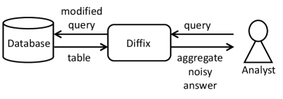
We base our definition of anonymity on these risks, not just because these definitions are used by practitioners, but also because 1) we find them to make sense intuitively, and 2) we can formulate tests that measure the risks. These definitions, however, imply an anonymization system that retains the notion of a “record”. Diffix-birch does not anonymize the dataset per se, but rather anonymizes answers to queries on the dataset: the analyst does not have direct access to the dataset and its records (Figure 2). We therefore modify these definitions to fit diffix-birch’s operational model as follows.

Refer to caption — Figure 2: Diffix-birch acts as an SQL proxy to an unmodified database

We define singling out as occurring when an analyst correctly makes a statement of the form “There is exactly one user that has these attributes.” For instance, the analyst may claim that there is a single user with attributes [gender = ’male’, age = 48, zipcode = 48828, lastname = ’Ng’]. If this is true, then the analyst has correctly singled out that user. The attributes don’t need to be personal attributes as in this example. If the analyst correctly claims that there is a single person with the geo-location attributes [long = 44.4401, lat = 7.7491, time = ’2016-11-28 17:14:22’], then that person is singled out.

We define linkability in the context of a second dataset (the linkability dataset) that has some users in common with the dataset behind diffix-birch (the protected dataset). In other words, for some fraction of rows in the linkability dataset, there are rows in the protected dataset that belong to the same user.

Assuming that the analyst has full access to the linkability dataset, linkability occurs when an analyst correctly makes a statement of the form “this user or set of users in the linkability dataset also exist in the protected dataset.”

We define inference in the context of a second dataset (the inference dataset) which is identical to the protected dataset, but where one or more cells in the inference dataset are masked (the values are unknown to the analyst). Other than this masking, the analyst has full access to the inference dataset.

Inference occurs when an analyst correctly makes a statement of the form “the value of this masked cell in the inference dataset is X”.

Of course, some fraction of an analyst’s claims may be incorrect. This leads to the notion of confidence, which is defined as the ratio of correct claims to all claims. If 95% of an analyst’s claims are correct, then the confidence of the attack is 95%. Confidence improvement (or just improvement for short) is the improvement in the analyst’s confidence over a statistical guess.

By way of example, suppose that roughly 90% of the users in the database have zipcode = 48828, and that the analyst knows this. Suppose also that the analyst has external knowledge that there is a single user with the attributes [gender = ’male’, age = 48, lastname = ’Ng’]. The analyst could simply claim that this user’s zipcode = 48828, and the analyst would have 90% confidence in the claim. But this does not improve on a statistical guess, and so Diffix-birch has not leaked additional information with respect to the inference. The improvement is therefore zero.

We measure confidence improvement as $\kappa=(C-S)/(1-S)$ , where $C$ is the analyst’s confidence, and $S$ is the statistical probability. So for example if the analyst were, through some attack on diffix-birch, to improve their confidence from 90% to 95%, then the confidence improvement would be $\kappa=0.5$ (or 50%).

The inference and linkability datasets imply some amount of externally derived prior knowledge. Our measure of the quality of diffix-birch’s anonymity accounts for this prior knowledge. Prior knowledge may be gained from external data sources, or the analyst may literally know portions of the database, for instance because a database that the analyst has full access to has been joined with other databases to form the protected database.

We define $P$ as the number of cells an analyst knows as prior knowledge, where a cell is a single value in the database (the value at a single column and row). Of course a cell may itself be a complex object with multiple values, but for our purposes we don’t worry about that. For singling out and inference attacks, we define $L$ as the number of cells an analyst learns. For linkability attacks, we define $L$ as the number of row linkages the analyst learns.

This allows us to define $\alpha=L/(P+1)$ as a value that expresses the strength of diffix-birch’s anonymization (or that of any anonymization scheme) with respect to the analyst’s prior knowledge. 1 is added to the denominator to avoid divide-by-zero.

Of course when an analyst “learns” something, it is with a certain confidence improvement $\kappa$ . Therefore, we characterize the strength of an anonymization scheme with both parameters $(\alpha,\kappa)$ . This strikes us as a reasonable though still flawed way for a privacy stakeholder, for instance a Data Protection Officer (DPO), to think about the value of an anonymization scheme. For instance, suppose that a given system has $(\alpha={10e-6},\kappa={0.9})$ . This means that an attacker must know a million things in order to learn one thing with a 90% confidence improvement. The DPO might or might not regard this as an acceptable risk, but at least the DPO will have some reasonable sense of the risk.

The reality of course is more complex. It may well be that knowing certain cells makes the system more attackable than knowing other cells. For instance, knowing all of a column that on its own isolates many users may be better for an attacker than knowing all of a column that isolates no users. It may also be that, given certain prior knowledge, certain cells are easier to learn than others. The sensitivity of the easier-learned cells may also be a factor.

What’s more, an $(\alpha,\kappa)$ score can only really be measured with respect to some specific attack. A DPO might therefore know be told something like “if an analyst knows columns A and B, and does a foobar attack, then he can learn things about column C with $(\alpha={10e-7},\kappa={0.85})$ ”.

Note that our immediate purpose for defining $(\alpha,\kappa)$ is in order to assign monetary payoffs in a bug bounty challenge. With respect to this paper at least, $(\alpha,\kappa)$ conveys a sense of how we think about measuring anonymity.

3.1 Limitations on GDPR anonymity criteria

Singling out: By our definition, a user is singled out even if an analyst makes a claim about a single cell value, as long as that value isolates the user and is not prior knowledge. There are cases, however, where the analyst may exploit specific patterns in the column data to make successful claims without in fact violating privacy in any meaningful way.

Common among these is the case where uid’s are assigned sequentially. Since the analyst knows that each uid is distinct, it is quite easy using diffix-birch to determine that the uid’s have been sequentially assigned, and roughly what the low and high uid values are. Given this, the analyst could make a series of singling out claims that there is one user with uid = 1, one user with uid = 2, and so on. Intuitively, we regard this as not violating privacy because it tells us nothing specific about the singled out user—one user could have a given uid as easily as the next.

We have no precise definition of when exploiting such predictable patterns in data are and are not privacy violating. For now we have to take these on a case-by-case basis.

Exposure of strings (security versus privacy):

It may be a security violation that any string in a database is revealed. For instance, if a column contains passwords, then it would likely be a security violation that any password is revealed, even if many users happen to have the same password. Neither diffix-birch nor the GDPR criteria for anonymity account for this requirement. If such a column exists in a database, then it must be removed or made inaccessible by diffix-birch.

4 Assumptions and terminology

Our system setup consists of an analyst that queries a database via diffix-birch (Figure 2). The database is conceptually a single table organized as rows and columns. The columns may be of any type, so long as there are equalities and inequalities defined for the type (e.g. column = value or column $<$ value) returning TRUE or FALSE. The database holds “raw” data: no perturbation on the values in the database is assumed, and no columns need be removed²²2 The exception is columns that are a security risk as opposed to a privacy risk, as with the password column example. , for instance those containing personally identifying information like names.

We refer to the entity whose privacy is being protected as the user. The user may well be a device like a smartphone or a vehicle or even an organization. We require that each database table with individual user data has a column containing user identifiers. This is typically nothing more than the Primary Key or Foreign Key in the relational database. By convention we call this column the uid. We assume that every distinct user has one and only one distinct uid. A user may of course have more than one row.

The database may change over time. However, to protect anonymity in the face of changes, all changes to the database must be timestamped, and all queries must have a time range associated with the query. Note that as of this writing, our implementation of Diffix-birch does not have mechanisms to ensure this.

Diffix-birch must be configured to know 1) which column contains the timestamps, and 2) which column contains the uid’s. No other data-specific configuration is required. Critically, the system operator need not understand the semantics or sensitivity of any other columns.

This paper assumes that each database table has only a single uid column, and that any given row contains information only about the user identified by the uid. This precludes certain data structures for social network data. For instance a row identifying both the sender and recipient of a message is disallowed. Rather, such a message would have to be encoded as two rows, one for the sender and one for the recipient.

Diffix-birch has no specific mechanisms to deal with perfect correlations between columns among groups of users. If such correlations exist, and there is a risk that an analyst knows of the correlation, then the amount of noise must be increased in proportion to the size of the correlated group. For instance, if 10 people in a geolocation database travel together as a group, then to protect the privacy of all users in the group the noise must be increased 10x. The noise amount is statically configured and applies to all answers.

An analyst may make an unlimited number of queries.

This paper does not address timing or other side-channel attacks.

5 Basic Design

A query may have zero or more filter conditions (or just conditions). The conditions determine which rows of the database comprise a given answer. A query may have one or more anonymizing aggregation functions. In diffix-birch, these include count, sum, avg, stddev, min, max, and median.

The query produces a response that consists of one or more columns, and zero or more rows or buckets. For example, the following query has two conditions (dept and salary), and one anonymizing aggregation function (count(*)). The response has two columns (salary and count(*)), and multiple buckets (response rows), where each bucket corresponds to a given salary. The dept condition excludes any database rows that don’t have a department of ’CS’, and the salary condition excludes any database rows from each bucket that do not have the salary corresponding to that bucket.

SELECT salary, count(*)

FROM hrtable

WHERE dept = ’CS’

GROUP BY salary

Diffix-birch distorts responses it two ways:

1.

It may change the aggregation function’s true value.
2.

It may suppress buckets.

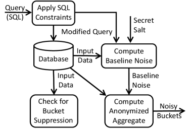
The change in aggregation function value is normally due in part to added pseudo-random noise taken from a Gaussian distribution. It may also in part be because of other mechanisms such as removing outliers from the input data (where input data here refers to the input of the aggregation function, see Figure 3). Bucket suppression happens when the input data for any given bucket has too few distinct users. For example, a bucket for the salary $100K that has a true value of 20 users may report a noisy value of 22 users. A bucket for the salary $450K that has only a single user will be completely suppressed.

5.1 Sticky Layered Noise

A key concept in diffix-birch is that of sticky layered noise. Diffix-birch’s noise is layered in that a bucket is not distorted by a single noise sample, but rather by the sum of multiple noise samples, where each sample is related to a condition.

Diffix-birch controls how a noise sample is generated by how it seeds the Pseudo-Random Noise Generator (PRNG): the same seed produces the same noise sample. Exactly how a seed is produced depends on the type of condition, but the general idea is to take aspects of the condition itself (the column name, the value, the operator), combine them with a secret salt, and use that as the seed.

In fact diffix-birch has two ways of seeding, or said differently, diffix-birch has two types of noise. We refer to these as static and dynamic noise. Static noise defends against averaging attacks, and dynamic noise defends against difference attacks (described further in this section).

As an example, the seed for the static noise layer associated with the condition WHERE dept=’CS’ in the above query is generated as³³3This is slightly simplified, see Section 6.5.:

static_seed =
   XOR(hash(concat(’hrtable’,’dept’,’CS’)),salt)

The difference between static and dynamic noise layers is that dynamic noise layers additionally include the distinct set of uid’s for the users whose rows comprise a given bucket. As such, the seed for the dynamic noise layer for the same condition would be:

dynamic_seed =
   XOR(static_seed,hash(uid1),hash(uid2),...)

Thus static noise layers are static in the sense that the same condition generates the same noise no matter what query it appears in, whereas a dynamic noise layer for a given condition will differ as long as the set of users in the bucket differ. For example, the static noise layers for dept=’CS’ in the following two queries are the same, while the dynamic noise layers will differ from each other so long as there are CS members younger than 30 or older than 40.

SELECT count(*)	SELECT count(*)
FROM hrtable	FROM hrtable
WHERE dept = ’CS’ AND	WHERE dept = ’CS’
age BETWEEN 30 AND 40

For queries that count distinct users, the standard deviation of each noise layer is $\sigma=1$ . As a result, a single noise layer taken alone introduces a fair amount of uncertainty as to the exact value of a distinct user count, and multiple noise layers even more so.

5.2 Attacks

With sticky layered noise, the simple averaging attack of Section 2 doesn’t work because the noise doesn’t change with each repeated bucket. The following sections explore additional attacks.

5.2.1 Split Averaging Attack

At this point one might suppose that noise needs to be sticky to prevent the averaging attack, but not necessarily layered. Here we describe a more sophisticated variant of the averaging attack, called the split averaging attack that justifies the need for layers.

In the split averaging attack, the analyst produces the pair of queries shown in Figure 4.

SELECT count(*)	SELECT count(*)
FROM table	FROM table
WHERE dept = ’CS’ AND	WHERE dept = ’CS’ AND
age = 20	age $<>$ 20

Figure 4: One pair of queries from a split averaging attack to learn exact count of people in the CS dept. Subsequent query pairs use age=21,22,...

The sum of the counts of the two queries gives the number of users in the CS department, plus noise (here assuming that there is one row per distinct uid). Now repeat the pair of queries, this time using age=21 and age<>21. This produces the same sum, but with different queries. The pairs can be repeated with age=22,23,24, and so on.

If noise were sticky but not layered, then each individual query would have a different noise sample because each query is different. With enough samples, the noise could be averaged away and a high-confidence exact count produced. Given exact counts, the analyst could then for instance carry out an intersection attack [4].

With static noise layers, however, the attack doesn’t work. Each query has two static noise values: one based on the condition dept=’CS’, and one based on the age condition (age=XX or age<>XX). The age-based noise value changes with each query, and so could be averaged away. The dept=’CS’ static noise, however, is always the same and is not averaged away. The final averaged count would be perturbed by the dept=’CS’ static noise layer.

5.2.2 Difference Attack

The split averaging attack explains the need for static noise layers, but not for dynamic noise layers. Indeed in the split averaging attack, all of the dynamic noise layers differ, even the one for dept=’CS’, because each bucket has a different uid set. Therefore they can also be averaged away and so don’t help defend against the split averaging attack. The following attack, called the difference attack, justifies the need for dynamic noise layers.

For this attack, suppose that an analyst happens to know that there is only a single woman in the CS department. Let’s call her the victim. The analyst could form the two queries shown in Figure 5.

SELECT salary, count(*)	SELECT salary, count(*)
FROM table	FROM table
WHERE dept = ’CS’ AND	WHERE dept = ’CS’
gender = ’M’	GROUP BY salary
GROUP BY salary

Figure 5: Difference attack to learn the isolated woman’s salary

Both queries produce a histogram of salary counts. The left query definitely excludes the victim from all answers. The right includes the victim only in the bucket that matches her salary. We refer to this as isolating the victim. Suppose we take the difference in the count between each bucket pair (two buckets representing the same salary). If we only had static noise layers, then this difference would be the same for every pair of buckets for a salary other than that of the victim. This is because the only difference between each such pair would the static noise layer for gender=’M’, which is always the same. However, the bucket pair representing the victim’s salary would have an additional difference: the count of the victim herself. As a result, to discover the victim’s salary, the attacker only needs to observe which bucket pair has a unique difference.

The dynamic noise layer defends against this attack. Because the set of uid’s differs between pairs of buckets, the difference in noise between each pair also differs. As a result, many pairs would exhibit a different difference, and the attacker would not know with certainty if the difference is due to a different count, or due to the dynamic noise layer.

5.2.3 Equations Attack

The equations attack from Section 2 requires that the amount of noise (the standard deviation of the noise) added to each sum be well below a certain threshold. We assume here that the equations attack also requires that each query has enough conditions to select the specific rows required by the attack: for each selected row, the query has to specify the set of attribute values that uniquely identify that row. Each such attribute value requires a condition, and each condition adds additional noise to the sum. Leaving out the details, in our experiments we found that the equations attack fails because too much noise is added to each sum.

5.2.4 Chaff Attacks

Section 2 briefly described a chaff attack on the simple sticky noise mechanism of Denning et.al. [3]. Because Denning’s sticky noise is based on the entire query, the attack only requires the addition, for instance, of a condition that has no effect on the rows in a bucket, i.e. age<>1000, age<>1001 etc. This specific simple chaff attack does not work with sticky layered noise because the additional condition only creates an additional noise layer, and doesn’t affect the other noise layers.

The attack on Denning’s sticky noise operates by changing the semantics of the query conditions, and exploits the fact that the semantic change happens not to effect the query result. A chaff attack that simply changes the syntax of the query would also work on Denning. For instance, the attacker could make a set of queries each with syntactically different but semantically identical conditions like age=50, age+1=51, age+2=52 and so on.

Whether semantic or syntactic chaff attacks work on diffix-birch depends entirely on what syntax is allowed in a query, and on how noise layers are computed from that syntax. The diffix-birch design in [10] specified a very simple syntax, allowing only conditions of the form column operator constant, where the operators were limited to =, <>, >, <, >=, and <=. No math, string or datetime functions, union semantics (OR), or JOIN’s among other things were allowed. Those constraints prevented syntactic chaff attacks: the semantics of a given query were always clear and sticky layered noise defended against semantic chaff attacks (to the best of our knowledge).

The design of diffix-birch in this paper allows a much richer subset of SQL, and therefore a much larger attack vector for chaff attacks. Chaff attacks are informally (and incompletely) addressed in other parts of this paper.

5.3 Bucket Suppression

Learning the strings or values that exist in a database is very useful. Simply listing a column’s values, however, violates singling out when any of the values belong to a single user. Therefore we wish to suppress any response where a value represented by a single user.

A simple mechanism for this would be to have a threshold for the number of distinct users that comprise a given bucket below which the bucket is suppressed. We need to take care, however, that the suppression or lack thereof doesn’t itself constitute a signal that might allow an analyst to obtain individual user information. For instance, a simple hard threshold, whereby all buckets with fewer than exactly $K$ distinct users is suppressed, can leak the presence of absence of a specific user in the case where the analyst knows that there are either $K$ or $K-1$ users with a given value. This $K$ th user is singled out in this case.

To avoid this, we use what we call a noisy threshold. This is a threshold whose value for any given bucket comes from a Gaussian distribution around a mean threshold. The noisy threshold used for bucket suppression, which we refer to as the low-count threshold, operates as follows.

If the number of distinct uid’s in the bucket is less than $T_{h}=2$ , then suppress the bucket. Otherwise, seed a sticky noise value $T_{n}$ with mean $\mu=4$ and standard deviation $\sigma=0.5$ using the distinct uid’s from the bucket:

  seed = XOR(salt,hash(uid1), hash(uid2), ...)

If the number of distinct uid’s in the bucket is less than $T_{n}$ , then suppress the bucket.

These specific values for $\mu$ , $\sigma$ , and $T_{h}$ are a matter of policy. It is overall good to ensure that the mean $\mu$ is three or four standard deviations from the hard threshold $T_{h}$ so that the hard threshold is rarely actually invoked and therefore can’t somehow be exploited. At the same time, it is safer to have a larger $\sigma$ , which then implies a larger mean. Unfortunately, the larger the mean, the more suppression. Often columns have a lot of distinct values that are populated by very few individuals, and much of this information can disappear when $\mu$ is too large. In addition, almost invariably analyst’s like to look at small groups, and so $\mu$ plays in important role in how fine-grained the analysis can be. Therefore, we select relatively small values for $\mu$ , $\sigma$ , and $T_{h}$ .

5.4 Baseline Noise and Noisy Threshold

The anonymizing aggregation functions use sticky layered noise it two ways: to add noise to the final answer, and to select groups of users using a noisy threshold. For both uses, diffix-birch uses noise from the summed static and dynamic noise layers described above. Specifically, diffix-birch produces a baseline noise value $N_{b}$ from which other noise values are derived as needed.

The mean of the baseline noise $N_{b}$ is $\mu_{base}=0$ , and its standard deviation is $\sigma_{base}=1$ . If a different mean or standard deviation is required for a given purpose, then the baseline noise is simply multiplied by a factor to obtain the required standard deviation, and the mean is adjusted accordingly.

For all of the noisy threshold uses in the anonymizing aggregation functions, the hard threshold is set to $T_{h}=2$ , and the noise value is set to $N_{b}/2+4$ (mean of 4).

5.5 Anonymizing Aggregation Functions

Diffix-birch implements the following anonymizing aggregation functions: count, sum, avg, stddev, min, max, and median. Each of these functions has a specific anonymization method that trades off the desire to minimize distortion against the goal of ensuring that the effect of any one individual in the bucket cannot be easily detected.

The functions count, sum, avg, and stddev are treated rather differently than the functions min, max, and median. This is because the former functions compute a value that is a composite of all values, whereas the latter functions compute a value that belongs to only a single user.

5.5.1 count, sum, avg, and stddev

The anonymization of these four functions are all based on that of sum. count is a sum of rows. avg is sum divided by count. stddev is ultimately derived from the avg function. Specifically for each row stddev computes the square of the difference between each value and the true average. It then computes the (anonymized) avg of these differences, and reports the square root of this avg.

There are two important but contradictory considerations to make when computing the anonymized sum. On the one hand, the amount of noise needs to be proportional to the largest contribution of any user. This is to protect against the case where a difference attack can isolate a user that contributes an unusually large amount to the sum.

SELECT sum(salary)	SELECT sum(salary)
FROM table	FROM table
WHERE dept = ’CS’ AND	WHERE dept = ’CS’
warn = 1 AND	warn = 1
gender = ’M’

Figure 6: Difference attack to learn whether the isolated woman has had a disciplinary warning given that she has a high salary.

For instance, consider the attack of Figure 6 which isolates the one woman in the CS department and tries to learn if she has had a disciplinary warning. She is excluded from the left query and included in the right if she has had a warning. Suppose that the amount of noise added is proportional not to the largest salary but to the average salary. Suppose also that the woman’s salary is substantially higher than the average, say $400K versus $125K. If the difference between the reported sums is around $400K or higher, then with very high probability the woman is present in the right-hand query and therefore has had a warning. This high probability comes from the fact that $400K is more than three standard deviations from $125K, so the probability that the difference is due purely to noise and not the contribution of the woman’s salary to the sum is very small.

On the other hand, making the noise proportional to the largest value causes a problem when that value is an outlier. For instance, suppose instead that the woman’s $400K salary in the attack of Figure 6 is twice that of the next highest salary, and that the analyst knows this fact. Now suppose that the reported sum of the right-hand query is $800K greater than that of the left-hand query. If the woman is present in the right-hand query, then this difference is due to her salary being included plus one standard deviation of noise. If the woman is not present in the right-hand query, then the difference would be due to four standard deviations of noise, a very low probability. Therefore the analyst can conclude with high probability that the woman has had a warning.

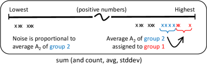
Therefore, to effectively hide any given user in a sum, it is necessary to first remove outliers, and then add noise proportional to the remaining highest values. Simply removing outliers, however, results in more distortion than necessary. Instead, we flatten the values of a few distinct users with the highest values (group 1 in Figure 7 so that they are comparable to those of the next few distinct users with the highest values (group 2).

The sum (and count) function has two phases, a pre-processing phase and a summing phase. The input to the summing phase is:

1.

A table with two columns, a uid column and a value column. The uid’s are distinct, and the value contains each user’s total contribution to the count or sum.
2.

A baseline sticky noise value $N_{b}$ derived from the noise layers (see Figure 3 and Section 5.4). $N_{b}$ has a standard deviation of $\sigma=\sqrt{L}$ , where $L$ is the number of noise layers. The actual noise is a multiplicative factor of $N_{b}$ .

Depending on the function, the pre-processing phase produces the value as follows:

count(distinct uid):: All values are ’1’.
count(*):: Each value is the number of rows for the uid.
count(column):: Same as count(*), except rows with NULL values are not counted.
count(distinct column):: Same as count(column), except duplicate values are removed before counting each user’s rows.
sum(column):: Each value is the sum of the values for the uid.
sum(distinct column):: Same as sum(column), except duplicate values are removed before summing each user’s values.

The summing phase consists of the following steps:

1.

Generate two noisy thresholds $T_{1}$ and $T_{2}$ (see Section 5.4).
2.

Label the $T_{1}$ distinct users with the highest values group 1.
3.

Label the $T_{2}$ distinct users with the next highest values group 2.
4.

Define $A_{2}$ as the average of the values from group 2.
5.

Replace the group 1 values with $A_{2}$ .
6.

Define $A_{all}$ as the average of all values (after replacement).
7.

Compute a noise value $N=N_{b}*max(1/2{A_{2}},A_{all}$ ).
8.

Sum the values, and add noise $N$ .

If there are both positive and negative values, then the above computations are done separately for the positive and negative values, using lowest values instead of highest. The actual added noise is the sum of the two noise values.

As described above, both the count(distinct column) and sum(distinct column) functions remove duplicate values during pre-processing. Duplicates are removed in such a way as to maximize the resulting number of distinct uid’s. This minimizes the contribution of any given user, allowing diffix-birch to minimize the noise.

Note that in the case of count(distinct uid), there is no distortion due to flattening. All values are 1, so the replacement in step 5 has no effect.

The reason in step 7 for computing the noise $N$ as proportional the max of the average of all values $A_{all}$ or one half the average of group 2 $A_{2}$ is to further lower the amount of noise in the case where the highest values are substantially higher than the average value. The premise here is that if the large values are substantially higher than the average, then there is some spread in the values contributed by different users, and therefore some uncertainty on the part of the analyst as to how much any given user is contributing to the sum. This uncertainty then reduces the need for the uncertainty inherent in the noise. This is admittedly at this time an unfounded premise, and more experimentation is needed to ensure that the premise is correct.

5.5.2 min, max, and median

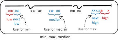
Since min and max in principle could report the value of an individual user, it is particularly important that the effect of extreme values are hidden. Diffix-birch removes noisy threshold numbers of distinct users from both the high and low end of the value range (see Figure 8). The average value of the next highest (lowest) noisy threshold number of distinct users are then used to compute max (min). Similarly, the median is computed from the average of the values of a noisy threshold number of distinct users above and below the true median.

Once the highest and lowest value are removed, max is computed as follows:

1.

Select a group of values from the values of a noisy threshold number of distinct (next) highest users.
2.

Compute the average $A$ of the group.
3.

Compute the standard deviation $\sigma$ of the group.
4.

The anonymized max value is computed as $A$ with added noise ${(N_{b}*{\sigma})}/8$ .

The computation of the noise amount in step 4 needs some explanation. $N_{b}$ is the noise value generated from the baseline noise. If all the values in the group are the same, then the standard deviation of the group is zero, and there is no noise added. In this case, the exact value of the group is reported. This is safe, because the group represents multiple distinct users and so any one user is hidden in the crowd. Furthermore, the analyst does not know how many users constitute the group. Indeed, if all the values in the averaged group and the removed group are identical, then max or min will report the correct true max or min.

If however, the values of the group are different, then we add a little noise to help ensure that the analyst cannot somehow reverse engineer the specific values in the group from the exact average $A_{2}$ . In fact, we don’t have evidence that this reverse engineering would be possible, but neither do we have evidence that it is not. So the noise is a fudge factor. With experimentation, we may find that it is not needed, or for that matter that it should be larger.

5.5.3 median

Like min and max, median can report the value of a single user, and can report the correct true median. Also like min and max, the values for the highest and lowest distinct users are first removed for computing median (see Figure 8). After that removal, the algorithm is as follows:

1.

Order the rows from highest to lowest values.
2.

Generate a noisy threshold $T$ (see Section 5.4).
3.

Select the true median row and label it.
4.

Label the rows for the $T$ distinct users above the true median, and the $T$ distinct users below the true median (the same user may appear once above and once below).
5.

Compute $A$ as the average of the labeled rows.
6.

Compute $\sigma$ as the standard deviation of the labeled rows.
7.

The anonymized median value is computed as $A$ with added noise ${(N_{b}*\sigma)}/8$ .

5.6 An Example

Figure 9 illustrates an example query in diffix-birch. The analyst requests the sum of salaries with two conditions (on columns dept and gender).

Diffix-birch processes the query, both to ensure that it conforms to the SQL restrictions placed by diffix-birch, and to modify the query so that the data required for anonymization is retrieved from the database. Both the low-count threshold and the anonymized sum function require the list of uid’s, and the sum function additional requires the list of salary values. As a result, the query is modified so as to request this data from the database. (Note that this is somewhat a simplification of what happens in our implementation.)

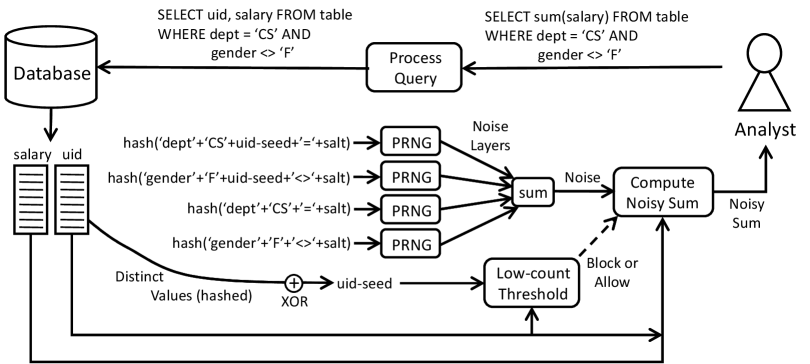
The contents of the uid column are used to generate the uid-seed for the low-count threshold check as well as for the dynamic noise layers. The low-count threshold check determines whether the bucket needs to be suppressed.

In this particular example, the seeds for the layered noise can be generated from examining the SQL itself. Two static and dynamic noise layers are generated, one each for the two conditions.

6 Details

The previous section describes the basic concepts of diffix-birch, giving examples for queries with simple conditions: AND’d conditions in a WHERE clause with no math or other functions. With the exception of a few updates, the concepts and examples essentially cover the material described in [10]. This section describes how diffix-birch is applied to a much richer SQL syntax.

The complete diffix-birch syntax is specified in Appendix A.

There are a number of restrictions on how the syntax specified in Appendix A may be used. As a rule, the purpose of these restrictions is to prevent an attacker from either generating conditions that diffix-birch does not recognize as conditions, or generating conditions whose semantics diffix-birch mis-interprets.

An example of the latter is given in Section 5.2.4, where for instance the conditions WHERE age=20, WHERE age+1=21, WHERE age+2=22 etc. are all semantically identical and so must produce the same noise layer.

An example of the former is the query shown in Figure 11, where the two queries both provide row counts of users age 30 or 40, but where the upper query has no explicit condition at all. We refer to attacks that emulate conditions without diffix-birch realizing it as backdoor attacks.

These restrictions are described throughout this section.

6.1 Terminology

A positive condition is one that includes rows that match the condition. For instance,

WHERE column = value
WHERE column IN (values)
WHERE column LIKE value

A negative condition is one that excludes rows that match the condition. For instance,

WHERE column <> value
WHERE column NOT IN (values)
WHERE column NOT LIKE value

An equality is a condition that requires an exact match to include or exclude rows. Diffix-birch has equality operators = and $<>$ .

An inequality is a condition with operators like less than or greater than. Diffix-birch places a restriction on inequalities in that the inequalities must express a range: both lower and upper inequality boundaries must be specified. Thus the condition WHERE age BETWEEN 10 AND 20 is allowed, but the condition WHERE age $<$ 20 is not allowed. Both positive and negative ranges may be expressed (i.e. BETWEEN and NOT BETWEEN).

A query condition may be clear or unclear. Simply put, a clear condition is one where diffix-birch understands the intent of the condition and can therefore derive the condition’s noise layers directly by examining the SQL. What passes as clear therefore depends on the sophistication of the diffix-birch SQL compiler (see Section 6.2 below).

6.2 Current scope of clear queries

As of this writing, the diffix-birch SQL compiler is not very sophisticated. To be considered clear, the column in the condition must either be the native column, or a native column being operated on by one of the following string operations: right, left, ltrim, rtrim, btrim, trim, substring, upper, or lower. To be considered clear, the condition must also have a simple constant (not operated on by math or any function). The upper four queries of Figure 10 are clear, while the bottom two are not.

SELECT sum(salary)	SELECT count(*)
FROM table	FROM table
WHERE left(date,4) = ’2009’	WHERE age = 64
SELECT avg(salary)	SELECT gender, count(*)
FROM table	FROM table
WHERE age	WHERE age
NOT IN (25,26,27)	BETWEEN 10 AND 20
SELECT sum(salary)	SELECT count(*)
FROM table	FROM table
WHERE left(date,4) $<>$ year	WHERE sqrt(age) = 8

Figure 10: The conditions for the top four queries are clear. The conditions for the bottom two are unclear.

The reason we specifically allow the string functions is because in our experience it is quite common for analysts to select sub-strings from a string. This is because strings frequently have an internal structure that the analyst wants to deconstruct (for instance a date encoded as a string, as in the example of Figure 10). In so doing we are conceptually treating the substring as a separate column. Nevertheless, when there is one of these string functions present, diffix-birch adds an extra noise layer to defend against potential attacks that try to exploit the function (Sections 6.13 and 6.14).

SELECT count(*), age_30_or_40 FROM (

SELECT uid,

(age_30 + age_40) % 2 as age_30_or_40 FROM (

SELECT uid,

floor((age_greater_29 + age_less_31) / 2) AS age_30,

floor((age_greater_39 + age_less_41) / 2) AS age_40

FROM (

SELECT

uid,

ceil((age - 29) / 100) AS age_greater_29,

ceil(0 - (age - 31) / 100) AS age_less_31,

ceil((age - 39) / 100) AS age_greater_39,

ceil(0 - (age - 41) / 100) AS age_less_41

FROM table

) x

) y

) z

GROUP BY age_30_or_40;

SELECT count(*)

FROM table

WHERE age = 30 OR age = 40

Figure 11: Backdoor Conditions: The upper and lower queries both produce counts of individuals aged 30 or 40. The upper query is disallowed by limiting the number of discontinuous functions combined with math and constants that may appear in a query.

Diffix-birch supports use of the HAVING clause in sub-queries. A HAVING clause necessarily implies an aggregation function and associated GROUP BY which must operate on the uid. Queries where this is not the case are rejected. The rules for when a HAVING clause is clear in the current implementation are the same as for the WHERE clause, with the exception that an aggregation function is allowed, and the constraint that the aggregation function must operate on a raw column value. For example, neither query of Figure 12 is considered clear. (Both would be clear if the +20 was removed.)

SELECT mxage, count(*)	SELECT mxage, count(*)
FROM (	FROM (
SELECT uid,	SELECT uid,
max(age) AS mxage	max(age+20) AS mxage
FROM table	FROM table
GROUP BY uid	GROUP BY uid
HAVING mxage+20 = 65)t	HAVING mxage = 65)t
GROUP BY mxage	GROUP BY mxage

Figure 12: Neither of these queries are clear, because of the math. Both would be clear if the +20 were removed.

6.3 AND’d conditions

In diffix-birch, the OR operation is not allowed. There is no fundamental reason for this. Indeed the IN operation, which has union semantics, is allowed.

A diffix-birch query consists of the intersection of a set of conditions, where the condition operators may be =, BETWEEN (or the equivalent pair of inequalities), IN, LIKE, IS NULL, and the corresponding negative variants (NOT IN etc.).

A diffix-birch query may have zero or more conditions. If a query has zero conditions, then a single dynamic noise layer is used. The seed components in this case consist of the table name, the hashed and XOR’d uid’s, and the secret salt.

When columns are selected, they are treated as positive AND’d conditions for the purpose of seeding noise layers. For instance, the left-hand query from Figure 13 generates a set of buckets, one for each unique pair of age and salary. For each pair of values, noise layers are seeded as though those values appeared in a WHERE clause (i.e. the query on the right).

SELECT age, salary, count(*)	SELECT count(*)
FROM table	FROM table
GROUP BY age, salary	WHERE age = 20 AND
	salary = 100000

Figure 13: Selected columns are implicitly AND’d positive conditions, and are treated as such for the purpose of seeding noise layers. The bucket produced by the left-hand query where age=20 and salary=100000 is seeded identically to that of the right-hand query.

Note that selected columns do not require an associated anonymizing aggregation function. For instance, the query on the left-hand side of Figure 14 is valid. In this case, however, for the purpose of anonymization the query is treated as though the count(*) anonymizing aggregation function were present. The only difference is in the layout of the query answer. For example, the answer to the right-hand query of Figure 14 would have a single row for each age. If the noisy count for age=20 from the right-hand query were 86, then the left-hand query would simply produce 86 rows each with age=20.

SELECT age	SELECT age, count(*)
FROM table	FROM table
	GROUP BY age

Figure 14: When no anonymizing aggregation function is present (left-hand query), then for the purpose of anonymization the query is treated as though count(*) was used (right-hand query).

6.4 Floating versus SQL Inspection

In Figure 9, diffix-birch is shown as requesting the uid column from the database in order to compute the uid seed component of the dynamic noise layers. We refer to this mechanism of requesting a column as floating the column. Every query requires that at least the uid column is floated. In the example of Figure 9, however, the other seed components are generated simply by inspecting the SQL itself. This is possible because the conditions in the query are clear.

There are cases, however, where the seed components cannot be derived from SQL inspection alone. One such case is that of selected columns being treated as implicit positive AND’d conditions as shown in Figure 13. The selected columns are floated and the values returned by the database are inspected and used as seed components.

Another example is where conditions are unclear. For instance, in the left-hand query of Figure 15, the condition WHERE age+1=26 is unclear because of the math. In this case, the age column is floated (along with the uid column) in order to compute the seed components of the noise layers for the age condition (right-hand query). In this case, the floated value for age used in the seed would be 25, which indeed captures the ”intent” of the condition. Floating gives the analyst access to a variety of math, string, and datetime operations while preventing chaff attacks that exploit those operations.

SELECT count(*)	SELECT uid, age
FROM table	FROM table
WHERE age+1 = 26	WHERE age+1 = 26

Figure 15: Because the condition is unclear, diffix-birch extracts and examines (floats) the column contents to derive the value seed component. When the analyst submits the left-hand query, diffix-birch transforms it to the right-hand query to extract the age column (and uid column) from the database.

In the case of a sub-query with a GROUP BY, the raw column cannot be floated because it no longer exists after the aggregation function. For instance in the left-hand query of Figure 16, the avg function in the sub-query transforms the individual rows into aggregate rows. It is therefore no longer possible to float the individual rows and use their values for seeding.

SELECT avtime, count(*)	SELECT uid, avtime, mn, mx, ct
FROM (	FROM (
SELECT uid,	SELECT uid,
avg(time) AS avtime	avg(time) AS avtime,
FROM taxi_rides	min(time) AS mn,
GROUP BY uid) t	max(time) AS mx,
GROUP BY avtime	count(time) AS ct
	FROM taxi_rides
	GROUP BY uid) t

Figure 16: The avg aggregation function in the analyst’s query (left side query) prevents floating the individual row values for the column time. Instead, min, max, and count aggregates are floated and used to seed noise layers (right side query).

One way to deal with this would be to somehow incorporate the aggregation function into the seed. For instance, for the left-hand query of Figure 16, the noise layer could additionally be seeded by the name of the aggregation function. The problem with this is that several aggregation functions can produce the same results. In any column where there is one row per distinct user, then min, max, avg, and median for instance all produce the same value. This allows the analyst to get four noise samples and so is a chaff attack, albeit limited by the number of different aggregation functions.

Rather, diffix-birch floats pre-specified aggregates, specifically min, max, and count, and uses the associated values in the seed. Pre-specified aggregates are chosen so that the analyst cannot influence what gets floated. These three particular aggregates are chosen because they work with numeric, text, and datetime column types, and at the same time provide good ”coverage” of the column contents.

The specific attack on HAVING that we want to avoid is one where the analyst isolates a user with two queries in such a way that the seeds for the noise layers associated with the aggregated column are the same. This could happen if the only difference between the two queries is the choice of aggregation function, the two aggregation functions change only a single row (that of the victim), but at the same time does not change the min, max, or count for the victim. While theoretically possible, we take it as a given that the probability of this occurring (and the analyst knowing it occurs) is negligible and does not need to be defended against.

6.5 Positive equality

Positive equalities are allowed. Positive equalities do not need to be clear. The seed components for the static noise layer, not including the salt, are:

   [table_name, column_name, value, value, 1]

If the condition is clear, then the value is simply extracted from the SQL and used to seed the noise layer. The same seed components are used whether the condition is in a WHERE or a HAVING clause. If the condition is not clear, then the column, or in the case of HAVING its min/max/count aggregates, is floated and the value is taken from the database.

The reason that the value is repeated, and the 1 included, can be explained as follows. Suppose that only a single instance of the value was used (i.e. [value] instead of [value,value,1] as is the case in the simplified seed description from Section 5.1, where value=’CS’). Suppose further than the table has one row per user. In that case, the analyst could compose a query containing an unclear HAVING that forces diffix-birch to float max/max/count aggregate values rather than the native column values. This would produce a seed that is different from that produced with the corresponding WHERE clause, thus giving the analyst another random sample. By using [value,value,1] instead of [value], the same seed results whether the analyst uses an unclear HAVING or a WHERE clause.

The seed for the dynamic layer of course additionally contains the XOR’d hashes of the uid’s. For brevity, in what follows unless otherwise specified we exclude the secret salt, table name, and column name from the specification of the static seed components, and additionally exclude the XOR’d hashes of uid’s from the specification of the dynamic seed components.

6.6 Negative equality

Negative equalities are allowed. Negative equalities must always be clear (in our current implementation). Examples of queries with negative equalities are the following:

SELECT count(*)	SELECT sum(salary)
FROM table	FROM table
WHERE age $<>$ 64	WHERE left(date,4) $<>$ ’2011’

The difficulty with generating seeds for negative conditions in general is that floating the column from the query as-is does not tell diffix-birch what the condition is excluding, but rather what happens to be included. In other words, SQL inspection of the condition WHERE age $<>$ 64 tells diffix-birch what the condition excludes, while floating of the age column tells diffix-birch what is included as a result of the negative condition.

To use floating (and therefore allow unclear conditions), diffix-birch would have to reverse the condition (change it from negative to positive), and probe the database with the modified query to determine what the condition is meant to exclude. For instance, the unclear condition on the left query below would be changed to the unclear condition on the right. An initial probe query would be made floating the age column. The value returned by the database would be 65, and this could then be used to seed the noise layer.

SELECT count(*)	SELECT count(*)
FROM table	FROM table
WHERE age+5 $<>$ 69	WHERE age+5 = 69

The decision to not implement a probing approach is simply one of prioritization. There is extra overhead (the additional query) and extra complexity. Given that in the future we can expand the set of queries that are clear with a smarter SQL compiler, the question of whether it is worth implementing a probing approach is still uncertain.

The seed components for the static noise layer include:

   [value]

Note that here there is no need to replicate the value and include 1. This is because there is no floating, and so never a need to float min/max/count.

6.7 Positive range

Inequalities must always be expressed as ranges. So the condition WHERE age BETWEEN 10 and 20 is allowed (or the equivalent using $>=$ and $<=$ ), but WHERE age $<=$ 20 alone (without a corresponding $>=$ ) is not allowed. The reason for this restriction is because of snapped alignment. Inequalities in diffix-birch are forced into a pre-determined (snapped) set of exponentially growing range sizes and offsets [10]. Numbers fall on intuitive boundaries like 0.1, 0.2, 0.5, 1, 2, 5, 10, 20, 50 etc., and datetimes fall on natural boundaries (second, hour, day etc.) and intuitive sub-boundaries. Simply put, in order to for a snapped size to be enforced, both edges of a range must be specified by the analyst.

Ranges must be clear. The seed components for the static noise layer include:

[lower_value, upper_value]

Note that if $>=$ , $<=$ syntax is used, then two conditions are treated as one.

The reason for snapped alignment is to prevent chaff attacks whereby the analyst repeats a series of queries, each with a slightly larger range, but in such a way that the small range change does not change the set of rows filtered by the condition. As a simple example, if the analyst knows that a given numerical column contains integers, the analyst could increase the range by increments of 0.01, thus obtaining many noise samples to average out.

As of this writing, we have no good ideas on how to allow unclear range queries. Unlike equalities, a range naturally allows a variety of different values to pass (those that fall in the range). If diffix-birch could deduce from floating the range’s column what the intended range is, then diffix-birch could 1) ensure that the range is snapped, and 2) use the range to seed the associated noise layers. The problem is that it is hard to deduce the intended range. For instance, suppose that diffix-birch observes values between 2 and 9 from floating the column. Diffix-birch cannot tell if the specified unclear range in the query is 0-10 and therefore properly snapped, or 2-9 and therefore not snapped, or even 0-20 because the range is properly snapped but just happens to have no values between 10 and 20.

6.8 Negative range

Negative ranges (i.e. NOT BETWEEN) are allowed. Negative ranges must of course also be clear. The seed components are identical to those for positive ranges, but with the addition of a symbol denoting that the range is negative:

[lower_value, upper_value, ’:<>’]

6.9 IN clause

The IN clause is equivalent to a series of OR’d positive equalities. For example, the following two queries are identical:

SELECT count(*)	SELECT count(*)
FROM table	FROM table
WHERE gen = ’M’ AND	WHERE gen = ’M’ AND
age IN (30,31)	(age = 30 OR age = 31)

The IN clause must be clear.

There are two ways in which an analyst could attempt a difference attack based on the IN clause. One is to remove the entire clause. Another is to remove or change one or more of the elements within the IN. As such, there are noise layers associated with the entire clause (the per-clause noise layers), and a noise layer associated with each element (the per-element noise layers).

Regarding the per-clause layer, diffix-birch creates a static noise layer (no dynamic layer) by floating the associated column. The noise layers are seeded with the following components:

[val1, val2, ...]

Where val1, val2 etc. are the floated column values. Note that if the IN clause has only a single element then it is treated identically to the corresponding positive equality (Section 6.5).

The reason that the IN column is floated, even though it is clear, is to defend against an averaging attack using chaff elements. For instance, if diffix-birch used SQL inspection to compose the per-clause noise layer, the analyst could submit a series of queries with age IN (50,1000), age IN (50,1001), etc.

Regarding the per-element noise layers, diffix-birch generates a dynamic noise layer for each element (no static layer). The seed components include:

[value]

where value is the element itself.

The reason we don’t require a per-clause dynamic noise layer is because any one of the per-element dynamic noise layers is effective in defending against a difference attack based on removing the clause.

The reason we don’t require a per-element static noise layer is because a set of per-element static noise layers, when summed together, behaves like a per-group static noise layer, but with more noise (a higher standard deviation). By having a single per-clause static noise layer, we reduce the total amount of noise.

6.10 NOT IN clause

A NOT IN clause is equivalent to a set of AND’d negative equalities. For example, the following two queries are equivalent.

SELECT count(*)	SELECT count(*)
FROM table	FROM table
WHERE age NOT IN (30,31)	WHERE age $<>$ 30 AND
	age $<>$ 31

Recognizing this, diffix-birch treats any NOT IN clause as its equivalent set of AND’d negative equality conditions (Section 6.6).

6.11 LIKE clause

The LIKE and ILIKE clauses enable a difference attack whereby a victim is isolated by exploiting a unique string associated with the victim. For example, suppose that the database has a column name consisting of last names. Suppose that the following conditions hold:

1.

The analyst has prior knowledge of the name column,
2.

the column contains a number of Murry’s (enough to avoid low-count filtering),
3.

the column contains a single McMurry,
4.

the column contains no other last names that end with Murry.

Under these conditions, the analyst could execute the difference attack on the victim McMurry with the queries shown in Figure 17. The left-hand query excludes McMurry while the right-hand query includes him or her because of the ’%’ wildcard symbol which matches on any zero or more of any character. As a result, whichever bucket matches McMurry’s gender will contain McMurry. LIKE also permits the ’_’ wildcard, which matches on exactly one of any character.

SELECT gender, count(*)	SELECT gender, count(*)
FROM table	FROM table
WHERE name LIKE ’Murry’	WHERE name LIKE ’%Murry’
GROUP BY gender	GROUP BY gender

Figure 17: In this difference attack, the LIKE comparator isolates the single McMurry in the case where there are multiple Murry’s.

Note that, at least with last names, the conditions for this attack exist surprisingly often. For instance, in a database of 250K last names with a distribution published by the US census, 0.2% of the names had the attack condition. Similar results were measured for Twitter hashtags.

Diffix-birch defends against this form of difference attack by more-or-less creating a noise layer per wildcard in the LIKE expression. The reason we do it this way, rather than try to create a single noise layer from the complete set of wildcards, is that it is too easy for an analyst to create chaff wildcard expressions otherwise. For instance, the expressions ’Mur_y’, ’Murr_’, ’Mu%rry’ etc. might all filter the same rows. If we had a single noise layer per expression each seeded differently, then the noise could be averaged out.

In creating the noise layers, we want to try to best capture the role that each wildcard plays in the expression. Note in particular that the ’%’ wildcard can often be inserted anywhere without having any effect on the filtered rows. For instance, suppose that the analyst wants to do the condition col LIKE ’abc_de’, but would like to average away the noise layer associated with the ’_’ wildcard using chaff. The analyst could try ’%abc_de’, ’%a%bc_de’, ’%ab%%c_de’, etc. It could well be that none of the ’%’ wildcards have any effect, but each new combination for instance pushes the ’_’ wildcard into a different string index position. Therefore we want to ensure that this kind of chaff attack also doesn’t work.

Our solution is to use the index position of the wildcard symbol to seed its associated noise layer, but to ignore ’%’ symbols when determining the index position. We also automatically ignore any repeated ’%’ symbols, since such symbols have no effect on the operation of the LIKE. The creation of the noise layers then takes the following steps:

1.
Modify the original expression by:
1. (a)
  
  Removing all repeating ’%’ symbols.
2. (b)
  
  Modifying any sequence of characters containing both ’%’ and ’_’ symbols to contain instead a single ’%’ at the beginning of the sequence, followed by the same number of ’_’ symbols.
2.
Generate a temporary expression by removing all ’%’ symbols, and:
1. (a)
  
  Compute $N$ as the number of characters in the temporary expression.
2. (b)
  
  Compute the index position $i$ of each character in the temporary expression.
3.
For each ’%’ symbol in the modified original expression, seed a noise layer using the following:
1. (a)
  
  $N$ .
2. (b)
  
  The position $i$ of the character preceding the ’%’ symbol.
3. (c)
  
  The symbol ’%’.
4.
For each ’_’ symbol, seed a noise layer using the following:
1. (a)
  
  $N$ .
2. (b)
  
  The position $i$ of the ’_’ symbol.
3. (c)
  
  The symbol ’_’.

As a result of this algorithm, the three expressions ’%abc_de’, ’%a%bc_de’, and ’%ab%%c_de’ all compute the same noise layer for the ’_’ symbol because the index position is always derived from the base string ’abc_de’. The apparnetly unavoidable downside of this approach is that it can create a lot of noise layers. Analysts must be aware of this and strive not to include unnecessary wildcards in LIKE expressions.

The LIKE clause must be clear.

6.12 NOT LIKE clause

The NOT LIKE and NOT ILIKE clauses must also be clear. NOT LIKE is seeded identically to LIKE, with the exception that the :not symbol is included as a seed component.

6.13 Character removing string functions

The current implementation of diffix-birch supports a number of string functions that can remove characters from the string. They include right, left, ltrim, rtrim, btrim, trim, and substring. All of these functions may appear in positive and negative conditions, including those that are otherwise clear. As a result, attacks similar to those for LIKE may be executed.

For instance, the condition WHERE right(name,5) = ’Murry’, which strips all characters but the last five, matches both Murry and McMurry. As another example, if a first name column contained multiple Paul’s but only one Paula, then both substring(name FROM 0 FOR 4)=’paul’ and WHERE left(name,4)=’Paul’. can be used to match both names.

For conditions containing these functions, an extra noise layer is created for the function. For example, given the condition WHERE right(name,5)<>’Murry’, the noise layers that would normally be created from the condition WHERE name $<>$ ’Murry’ would be created, and in addition a dynamic noise layer specifically associated with the right function would be created.

This extra dynamic noise layer has the following seed components:

•

The function name
•

The constant (or constants, in the case of substring) associated with the function (i.e. the number 5 in the case of right(name,5))
•

The symbol : $<>$ if a negative condition

In the case of trim, we use ltrim, rtrim, or btrim as the function name depending on whether the trim is LEADING, TRAILING, or BOTH.

In the case of substring(col FOR X) or substring(col FROM 0 FOR X), then we treat it as the equivalent left(col, X) with respect to seeding.

The constant for the trim’s needs to be normalized so that the analyst can’t add chaff and average out the noise by for instance scrambling the characters or adding extra redundant characters. To do this, we remove redundant characters and put the characters in alpha-numeric order.

6.14 String functions lower and upper

The current implementation also supports the string functions lower and upper. While these to our knowledge cannot be used in a difference attack, without additional noise layers they could in many cases be used in a limited chaff attack to obtain three static noise samples for the same query. For instance, suppose that the first letter of last names is capitalized. The analyst could obtain three noise samples with the following three conditions:

WHERE name <> ’Smith’
WHERE upper(name) <> ’SMITH’
WHERE lower(name) <> ’smith’

When upper or lower appears in a positive equality or with the IN comparator, then nothing special is required to seed the associated noise layers. The column is floated (prior to the case change) and handled as usual.

When they appear in a condition that does not float (negative equality or NOT IN) then an extra static noise layer is generated. This noise layer is the same regardless of whether the analyst executes upper or lower: diffix-birch forces the string to lower case for the purpose of seeding the noise layer. As such, seed components include:

[lower(value), ’:<>’, ’:lower’]

where lower(value) is the string in lower case, and :lower is an extra symbol.

6.15 Functions that produce ranges

There are a number of functions that, when combined with a condition, effectively produce ranges. For instance, Figure 18 show how trunc and year mimic the corresponding ranges specified with BETWEEN. These include all of the datetime functions in Appendix B.2, and the math functions trunc and round.

SELECT count(*)	SELECT count(*)
FROM table	FROM (
WHERE age	SELECT uid,
BETWEEN 10 AND 20	trunc(age, -1) AS tr_age
	FROM table) t
	WHERE tr_age = 10
SELECT count(*)	SELECT count(*)
FROM table	FROM (
WHERE date	SELECT uid,
BETWEEN ’2016-01-01’	year(date) AS yr
AND ’2016-12-31’	FROM table) t
	WHERE yr = 2016

Figure 18: A variety of math and datetime functions can group rows as ranges. Here the query on the left and right of each pair produce the same results (using trunc and year respectively).

Without getting into details, our implementation recognizes these functions and associated conditions as requiring the same noise layers as their explicit counterparts. Note that all of the functions listed above are ”naturally” snapped. trunc and round operate on powers of 10 (0.01, 0.1, 1, 10, …), and with the exception of weekday and quarter, the datetime functions operate on the same natural datetime boundaries as diffix-birch’s snapped alignment. Note that strictly speaking there are other math functions like floor and ceil, and even casting a real to an int, that also can generate ranges. These, however, only operate at the level of single integers, and so we feel provide inadequate expressiveness from which to effectively be used for attacks.

6.16 Function concat

Diffix-birch allows the function concat. concat can be used to mimic AND’d positive conditions. For instance, the two queries in Figures 19 produce the same buckets.

SELECT bday,age,	SELECT concat(c_bday, ’-’, c_age),
count(*)	count(*)
FROM table	FROM (SELECT uid,
GROUP BY bday,age	cast(bday, text) AS c_bday,
	cast(age, text) AS c_age
	FROM table) t
	GROUP BY concat(c_bday, ’-’, c_age)

Figure 19: The concat function can be used to mimic positive AND’d conditions. The above queries produce identical buckets.

Diffix-birch floats the columns used by concat and generates noise layers identical to those produced by positive AND’d conditions.

6.17 Noise reporting functions

In order to help the analyst gauge the accuracy of query results, diffix-birch provides a number of functions that report the amount of the added noise (the standard deviation). Especially for functions that report sums or the count of rows, the amount of noise may vary substantially since it is proportional to the contribution of some of the largest users. These functions are count_noise, sum_noise, avg_noise, and stddev_noise.

Since the noise amount is itself based on values from multiple distinct users, we do not expect it to be attackable. Never-the-less, to stay on the safe side, the reported noise is a rounded value. The unit of rounding increases with the size of the standard deviation such that the rounded value is within roughly 5% of the true value.

References

[1] European Union Article 29 Data Protection Working Party Opinion 05/2014 on Anonymization Techniques.
[2] Aggarwal, C. C. On k-anonymity and the curse of dimensionality. In Proceedings of the 31st International Conference on Very Large Data Bases (2005), VLDB ’05, VLDB Endowment, pp. 901–909.
[3] Denning, D. E. Secure statistical databases with random sample queries. ACM Transactions on Database Systems (TODS) 5, 3 (1980), 291–315.
[4] Denning, D. E., Denning, P. J., and Schwartz, M. D. The tracker: A threat to statistical database security. ACM Transactions on Database Systems (TODS) 4, 1 (1979), 76–96.
[5] Dinur, I., and Nissim, K. Revealing information while preserving privacy. In Proceedings of the twenty-second ACM SIGMOD-SIGACT-SIGART symposium on Principles of database systems (2003), ACM, pp. 202–210.
[6] Dwork, C. Differential Privacy: A Survey of Results. In TAMC (2008), pp. 1–19.
[7] Erlingsson, Ú., Pihur, V., and Korolova, A. Rappor: Randomized aggregatable privacy-preserving ordinal response. In Proceedings of the 2014 ACM SIGSAC conference on computer and communications security (2014), ACM, pp. 1054–1067.
[8] Fellegi, I., and Phillips, J. Statistical confidentiality: Some theory and application to data dissemination. In Annals of Economic and Social Measurement, Volume 3, number 2. NBER, 1974, pp. 399–409.
[9] Fellegi, I. P. On the question of statistical confidentiality. Journal of the American Statistical Association 67, 337 (1972), 7–18.
[10] Francis, P., Probst Eide, S., and Munz, R. Diffix: High-Utility Database Anonymization. Springer International Publishing, Cham, 2017, pp. 141–158.
[11] George Gatewood. A Monograph on Confidentiality and Privacy in the U.S. Census, July 2001.
[12] Sweeney, L. k-anonymity: A model for protecting privacy. International Journal of Uncertainty, Fuzziness and Knowledge-Based Systems 10, 05 (2002), 557–570.
[13] Tang, J., Korolova, A., Bai, X., Wang, X., and Wang, X. Privacy loss in apple’s implementation of differential privacy on macos 10.12, 2017.

Appendix A Complete Diffix-birch SQL Syntax

SELECT [DISTINCT]
  field_expression [, ...]
  FROM from_expression [, ...]
  [ WHERE where_expression [AND ...] ]
  [ GROUP BY column_expression | position [, ...] ]
  [ HAVING having_expression [AND ...] ]
  [ ORDER BY column_name [ASC | DESC] | position [, ...] [ LIMIT amount ] [ OFFSET amount ] ]

field_expression :=
  * | table_name.* | column_expression [AS alias]

column_expression :=
  [table_name.]column_name |
  aggregation_function([DISTINCT] column_name) |
  function(column_expression) |
  column_expression binary_operator column_expression |
  column_expression::data_type

binary_operator :=
  + | - | * | / | ^ | %

data_type :=
  integer | real | text | boolean | datetime | date | time

from_expression :=
  table | join

table :=
  table_name [[AS] alias] | (select_expression) [AS] alias

join :=
  table CROSS JOIN table |
  table { [INNER] | { LEFT | RIGHT } [OUTER] } JOIN table ON where_expression

aggregation_function :=
  COUNT | SUM | AVG | MIN | MAX | STDDEV | MEDIAN

where_expression :=
  column_expression equality_operator (value | column_expression) |
  column_expression inequality_operator (numerical_value | datetime_value) |
  column_expression BETWEEN value AND value |
  column_expression IS [NOT] NULL |
  column_expression [NOT] IN (constant [, ...])
  column_expression [NOT] LIKE | ILIKE string_pattern [ESCAPE escape_string]

having_expression :=
    column_expression comparison_operator (value | column_expression)

comparison_operator :=
    equality_operator | inequality_operator

equality_operator :=
    = | <>

inequality_operator :=
    > | >= | < | <=

Appendix B Diffix-birch Supported Functions

B.1 String Functions

•

BTRIM()
•

CONCAT()
•

HEX()
•

LEFT()
•

LENGTH()
•

LOWER()
•

LCASE()
•

LTRIM()
•

RIGHT()
•

RTRIM()
•

SUBSTRING()
•

TRIM()
•

UPPER()
•

UCASE()

B.2 Datetime Functions

•

year()
•

quarter()
•

month()
•

day()
•

hour()
•

minute()
•

second()
•

weekday()
•
EXTRACT()
- –
  
  year
- –
  
  quarter
- –
  
  month
- –
  
  day
- –
  
  hour
- –
  
  minute
- –
  
  second
•
DATE_TRUNC()
- –
  
  year
- –
  
  quarter
- –
  
  month
- –
  
  day
- –
  
  hour
- –
  
  minute
- –
  
  second

B.3 Math Functions

Operators +, -, *, /, ,̂ and %.

•

ABS()
•

BUCKET()
•

CEIL()
•

DIV()
•

FLOOR()
•

MOD()
•

POW()
•

ROUND()
•

SQRT()
•

TRUNC()

B.4 Noise Indicators

•

count_noise()
•

sum_noise()
•

avg_noise()
•

stddev_noise()

B.5 Casting

The following tables indicate what casting combinations are allowed.

Casting
from/to	text	integer	real	boolean
text	X	X	X	X
integer	X	X	X	X
real	X	X	X	X
boolean	X	X	X	X
date	X
time	X
datetime	X
interval	X

Casting
from/to	date	time	datetime	interval
text	X	X	X	X
integer
real
boolean
date	X
time		X
datetime	X	X	X
interval				X