Dynamically Rescaled Hamiltonian Monte Carlo for Bayesian Hierarchical Models

Abstract

Dynamically rescaled Hamiltonian Monte Carlo (DRHMC) is introduced as a computationally fast and easily implemented method for performing full Bayesian analysis in hierarchical statistical models. The method relies on introducing a modified parameterisation so that the re-parameterised target distribution has close to constant scaling properties, and thus is easily sampled using standard (Euclidian metric) Hamiltonian Monte Carlo. Provided that the parameterisations of the conditional distributions specifying the hierarchical model are “constant information parameterisations” (CIP), the relation between the modified- and original parameterisation is bijective, explicitly computed and admit exploitation of sparsity in the numerical linear algebra involved. CIPs for a large catalogue of statistical models are presented, and from the catalogue, it is clear that many CIPs are currently routinely used in statistical computing. A relation between the proposed methodology and a class of explicitly integrated Riemann manifold Hamiltonian Monte Carlo methods is discussed. The methodology is illustrated on several example models, including a model for inflation rates with multiple levels of non-linearly dependent latent variables. Supplementary materials are available online.

1 Introduction

The modelling of dependent data is routinely carried out using Bayesian hierarchical models in a diverse range of fields. The application of non-linear/non-Gaussian hierarchical models requires numerical methods for computing posterior distributions, predictions and so on, and with the demand for ever more complex and high-dimensional models comes also the demand for ever more capable numerical methods for tackling such models.

Current state of the art numerical methods for Bayesian hierarchical models fall roughly into two categories. The first category involves methods based on integrating out latent variables using variants of the Laplace approximation (see e.g. Rue et al., 2009; Kristensen et al., 2016). Such methods are extensively used, as they are computationally fast and can be applied by non-experts in computational statistics. However, such methods are also of fixed approximation accuracy and are somewhat restricted with respect to the models that can be handled. The second category contains several variants of Markov chain Monte Carlo (MCMC) (see e.g. Liu, 2001; Robert and Casella, 2004; Gelman et al., 2014). Early applications of MCMC to non-linear/non-Gaussian Bayesian hierarchical models (see e.g. Jacquier et al., 1994) typically relied on Gibbs sampling, but by now, it is well known that such Gibbs samplers, as a consequence of strong, non-linear dependencies between parameters and latent variables, typically mix very slowly. Recent trends in MCMC for hierarchical models have involved various methods targeting the marginal posterior distribution of the parameters only (Fernandez-Villaverde and Rubio-Ramirez, 2007; Andrieu et al., 2010; Flury and Shephard, 2011). Such methods have the potential for fast mixing, but also rely on a high quality Monte Carlo estimate of the said parameter posterior marginal that is often both very computationally demanding and may require bespoke implementations for each model instance.

Recently, Hamiltonian Monte Carlo (HMC) (Duane et al., 1987; Neal, 2010) has seen widespread use in many MCMC applications in statistics; in large part as such can produce close to iid chains while only requiring the ability to evaluate- and calculate the gradient of the target log-density. In particular, the No U Turn Sampler (NUTS) (Hoffman and Gelman, 2014), a variant of HMC, allows for automatic tuning. NUTS has seen widespread use as it is the default MCMC algorithm in the statistical software and modelling language Stan (Carpenter et al., 2017). However, as explained in e.g. Betancourt (2013); Kleppe (2018), direct application of HMC may work poorly or lead to misleading results when applied to (joint parameters and latent variables) target distributions associated with Bayesian hierarchical models, as such targets typically involve strong non-linearities, and in particular substantially different scaling properties across the support.

By adapting to the local scaling properties of the target, Riemann manifold Hamiltonian Monte Carlo (RMHMC) (see e.g. Girolami and Calderhead, 2011; Lan et al., 2015) holds the promise for high fidelity MCMC even for such complicated high-dimensional target distributions. RMHMC can also be made rather automatic by extracting scaling information from the negative Hessian of the target log-density (Betancourt, 2013; Kleppe, 2018). However, RMHMC may be very computationally demanding, in large part due to the need for solve a large number of high-dimensional sets of non-linear equations in each MCMC iteration.

The present paper seeks to combine the highly automatic and computationally fast nature of the HMC (here the Stan NUTS implementation is used) with variable scaling-respecting nature of RMHMC. This is accomplished by introducing a bijective mapping between the original parameterisation and a modified parameterisation with globally near-constant scaling properties. The said mapping combines information from priors and observations. Subsequently, HMC is applied in the modified parameterisation. The resulting MCMC method is referred to as dynamically rescaled HMC. Care is taken to ensure that, while retaining that the mapping reflects the variable scaling properties under the original parameterisation, the said bijective mapping is explicit. By exploiting sparsity originating from conditional independence assumptions in linear algebra, the methodology is computationally fast.

Two concepts, which together ensures the existence of said bijection, namely sequentially dependent block-diagonal scaling matrices/metric tensors and constant (Fisher) information parameterisations are discussed in detail. The approach taken here has some similarities with Zhang and Sutton (2014) in that analytical and numerical tractability introduced by working with block-diagonal metric tensors under a RMHMC framework is exploited. However, the approaches are distinguished by that different assumptions are imposed on the metric tensor, and that the Hamiltonian dynamics considered here uses a Euclidian metric (which admit implementation of the proposed methodology in standard software), whereas Zhang and Sutton (2014) is based on a Riemann manifold metric and a non-standard symplectic integrator. Furthermore, the present work also has some similarities to transport map accelerated MCMC (Parno and Marzouk, 2018) in that a modified, more easily sampled target is constructed via a bijective mapping. However, the approach taken by Parno and Marzouk (2018) for constructing such a mapping is based on MCMC output and a semi-parametric method, whereas in the present work, the mapping is constructed based on the model components in a parametric manner.

The rest of this paper is laid out as follows: Section 2 fixes notation and discusses HMC and HMC applied to hierarchical models in more detail. Section 3 discusses DRHMC based on sequentially dependent block diagonal scaling matrices, and details an interesting relation between DRHMC and RMHMC. In Section 4, specific sequentially dependent block diagonal scaling matrices, obtained using constant information parameterisations, are developed. Section 5 illustrates and benchmarks the methodology for some simpler models, and Section 6 applies the methodology to the challenging Stock and Watson (2007) inflation rate model. Finally, Section 7 provides a discussion.

2 Setup and background

First, some notation is fixed: The $n\times m$ zero matrix ($n$-dimensional zero vector) is denoted by $\mathbf{0}_{n,m}$ ($\mathbf{0}_{n}$), and the $n\times n$ identity matrix is denoted $\mathbf{I}_{n}$. A matrix $\mathbf{A}\in\mathbb{R}^{d\times d}$ is said to be block diagonal with square blocks $\{\mathbf{A}_{(r)}\}_{r=1}^{R},\;\mathbf{A}_{(r)}\in\mathbb{R}^{d_{(r)}\times d_{(r)}}$ if $\sum_{r=1}^{R}d_{(r)}=d$ and

$$\mathbf{A}=\left[\begin{array}[]{cccc}\mathbf{A}_{(1)}&\mathbf{0}_{d_{1},d_{2}}&\cdots&\mathbf{0}_{d_{1},d_{R}}\\ \mathbf{0}_{d_{2},d_{1}}&\mathbf{A}_{(2)}&\cdots&\mathbf{0}_{d_{2},d_{R}}\\ \vdots&\vdots&\ddots&\vdots\\ \mathbf{0}_{d_{R},d_{1}}&\mathbf{0}_{d_{R},d_{2}}&\cdots&\mathbf{A}_{(R)}\end{array}\right].$$

The notation $\mathbf{A}=\text{bdiag}(\mathbf{A}_{(1)},\dots,\mathbf{A}_{(R)})$ for such a matrix. The notation $\mathbf{A}>0$ signifies that $\mathbf{A}$ is a symmetric and positive definite (SPD) matrix. For a scalar quantity $a(\mathbf{x}),\;\mathbf{x}\in\mathbb{R}^{n}$, then $\nabla_{\mathbf{x}}a(\mathbf{x})\in\mathbb{R}^{n}$ denotes the gradient of $a$ with respect to $\mathbf{x}$, and for a vector-valued quantity $\mathbf{b}(\mathbf{x})\in\mathbb{R}^{m}$, $\nabla_{\mathbf{x}}\mathbf{b}(\mathbf{x})\in\mathbb{R}^{m\times n}$ is the Jacobian of $\mathbf{b}$. In what follows, it is assumed that the target distribution has a sufficiently smooth density $\mathbf{\pi}(\mathbf{q})$ and associated density kernel $\tilde{\pi}(\mathbf{q})$ (that can be evaluated) on the space of parameters $\mathbf{q}\in\Omega\subseteq\mathbb{R}^{d}$. All Gamma-distributions are in rate parameterisation unless otherwise noticed.

2.1 Hamiltonian Monte Carlo

(Euclidian metric) HMC (see e.g. Neal, 2010, for a detailed description) relies on defining a synthetic Hamiltonian (i.e. energy conserving) dynamical system that evolves over time $t$ so that the position coordinate $\mathbf{q}\in\Omega$ preserves the target distribution $\pi(\mathbf{q})$ for any time increment. Such a system may be found by specifying the total energy in the system (up to an additive constant), namely the Hamiltonian, as

$$\mathcal{H}(\mathbf{q},\mathbf{p})=-\log\tilde{\pi}(\mathbf{q})+\frac{1}{2}\mathbf{p}^{T}\mathbf{M}^{-1}\mathbf{p},$$ (1)

where $\mathbf{p}\in\mathbb{R}^{d}$ is the momentum variable and $\mathbf{M}>0$ is the mass matrix which can be chosen freely. The time-dynamics of $(\mathbf{q}(t),\mathbf{p}(t))$ solve Hamilton’s equations

$$\frac{d}{dt}\mathbf{q} =\nabla_{\mathbf{p}}\mathcal{H}(\mathbf{q},\mathbf{p})=\mathbf{M}^{-1}\mathbf{p},$$ (2)

$$\frac{d}{dt}\mathbf{p} =-\nabla_{\mathbf{q}}\mathcal{H}(\mathbf{q},\mathbf{p})=\nabla_{\mathbf{q}}\log\tilde{\pi}(\mathbf{q}).$$ (3)

The time dynamics associated with (2,3) preserves total energy of the system (i.e. $\frac{d}{dt}\mathcal{H}(\mathbf{q}(t),\mathbf{p}(t))=0$) and also the Boltzmann distribution $\pi(\mathbf{q},\mathbf{p})\propto\exp(-\mathcal{H}(\mathbf{q},\mathbf{p}))$. I.e. if $(\mathbf{q}(0),\mathbf{p}(0))\sim\pi(\mathbf{q},\mathbf{p}),$ then also $(\mathbf{q}(t),\mathbf{p}(t))\sim\pi(\mathbf{q},\mathbf{p})\;\forall\;t$. Moreover, since $\mathbf{q}$ and $\mathbf{p}$ are independent under the Boltzmann distribution associated with (1), it is clear that the original target is $\mathbf{q}$-marginal of the Boltzmann distribution.

In practice, for all but the most analytically tractable targets, the dynamics associated with Hamilton’s equations must be simulated numerically. To this end, the Størmer-Verlet or leap frog integrator is most commonly used to approximately advance the dynamics from time $t$ to time $t+\varepsilon$ via:

$$\mathbf{p}(t+\varepsilon/2) =\mathbf{p}(t)+\frac{\varepsilon}{2}\nabla_{\mathbf{q}}\log\tilde{\pi}(\mathbf{q}(t)),$$ (4)

$$\mathbf{q}(t+\varepsilon) =\mathbf{q}(t)+\varepsilon\mathbf{M}^{-1}\mathbf{p}(t+\varepsilon/2),$$ (5)

$$\mathbf{p}(t+\varepsilon) =\mathbf{p}(t+\varepsilon/2)+\frac{\varepsilon}{2}\nabla_{\mathbf{q}}\log\tilde{\pi}(\mathbf{q}(t+\varepsilon)),$$ (6)

This integrator is (time-) reversible and volume preserving (see e.g. Leimkuhler and Reich, 2004), but the output does not preserve the Hamiltonian (total energy). To correct for this discrepancy between the true and numerically integrated dynamics, an accept-reject step is included to complete the basic HMC algorithm for generating samples $\{\mathbf{q}^{i}\}_{i}\sim\pi(\mathbf{q})$ via repeating the steps:

• Sample new momentums $\mathbf{p}(0)\sim N(\mathbf{0},\mathbf{M})$ and set $\mathbf{q}(0)=\mathbf{q}^{i}$.

• Starting at $(\mathbf{q}(0),\mathbf{p}(0))$, perform $L$ leap frog steps with step size $\varepsilon$ to obtain proposal $(\mathbf{q}(L\varepsilon),\mathbf{p}(L\varepsilon))$.

• Set $\mathbf{q}^{i+1}=\mathbf{q}(L\varepsilon)$ with probability $\min[1,\exp\{\mathcal{H}(\mathbf{q}(0),\mathbf{p}(0))-\mathcal{H}(\mathbf{q}(L\varepsilon),\mathbf{p}(L\varepsilon))\}]$ and set $\mathbf{q}^{i+1}=\mathbf{q}^{i}$ with remaining probability.

Many improved variants of the HMC exist. Most notable is NUTS (Hoffman and Gelman, 2014), which chooses the number of integration steps $L$ dynamically. In addition, NUTS also involves a dual averaging algorithm for choosing $\varepsilon$.

Still, the choices of time step size $\varepsilon$ and mass matrix $\mathbf{M}$ influence substantially the performance of HMC. The mass matrix must be chosen so that the resulting $\mathbf{q}$-dynamics traverses the relevant parts of the support of $\pi(\mathbf{q})$ in a coherent and non-oscillating manner, and also ensures that the resulting HMC method is appropriately scaled. For near-Gaussian targets, a rule of thumb (Neal, 2010) is that $\mathbf{M}$ should be chosen to be close to the precision matrix of $\pi(\mathbf{q})$, but for highly non-Gaussian targets, the picture is less clear.

The performance also depends on the integrator step size $\varepsilon$. Too small $\varepsilon$s lead to high acceptance probabilities in the HMC algorithm, but also to that too many integration steps (with fixed computational cost roughly equal to that of $\nabla_{\mathbf{q}}\log\tilde{\pi}(\mathbf{q})$) must be performed to traverse the relevant parts of the target. Too large $\varepsilon$s, on the other hand, lead to inaccurate representation of the true dynamics and consequently a poor acceptance rate in the accept-reject step.

2.2 HMC and Bayesian hierarchical models

HMC, when properly tuned, can be extremely efficient on targets where the log-density has close to constant curvature (leading to close to linear differential equations (2,3)), even in high dimensions. However, when the target is the joint parameters-and-latent variables posterior in Bayesian hierarchical models, the performance of HMC may in many cases be very poor and HMC may produce misleading results when shorter MCMC runs are performed (see e.g. Kleppe, 2018).

Such poor performance is at least to some degree caused by that the local scaling properties of the target may change by several orders of magnitude across the relevant support of the target in this case. The behaviour arises, for instance, when latent variables and a variance parameter associated with the latent variables are considered jointly (see e.g. Kleppe, 2018, Figure 1). In such situations, the global scaling induced by choosing fixed $\mathbf{M}$ and $\varepsilon$ may require a very defensive scaling, which is only efficient for the most extremely scaled subsets of $\Omega$, and consequently may be very computationally wasteful in the remaining subsets of $\Omega$.

Unlike strategies based on varying $\mathbf{M}$ across the target support (e.g. Girolami and Calderhead, 2011) to counteract variable scaling, the approach of the present paper is to change the target distribution so that the resulting, modified target has close to constant curvature. Subsequently, HMC can be successfully applied to the modified target and MCMC samples distributed according to the original target may be easily recovered.

3 Dynamically rescaled HMC methods based on sequentially dependent block diagonal scaling matrices

3.1 Dynamically rescaled HMC methods

Dynamically rescaled HMC methods takes as vantage point a smooth, bijective transformation $\Psi:\mathbb{R}^{d}\mapsto\Omega$ and the introduction of modified parameterisation $\bar{\mathbf{q}}$ so that $\mathbf{q}=\Psi(\bar{\mathbf{q}})$. Based on these constructions, the modified Hamiltonian

$$\mathcal{H}_{DR}(\bar{\mathbf{q}},\mathbf{p})=-\log\tilde{\pi}(\Psi(\bar{\mathbf{q}}))-\log(|\nabla_{\bar{\mathbf{q}}}\Psi(\bar{\mathbf{q}})|)+\frac{1}{2}\mathbf{p}^{T}\mathbf{M}^{-1}\mathbf{p},$$ (7)

is considered. I.e. $\mathcal{H}_{DR}(\bar{\mathbf{q}},\mathbf{p})$ allows regular HMC sampling, but with modified target distribution $\propto\tilde{\pi}(\Psi(\bar{\mathbf{q}}))|\nabla_{\bar{\mathbf{q}}}\Psi(\bar{\mathbf{q}})|$, and thus with $\Psi(\bar{\mathbf{q}})$ being distributed according to the original target distribution $\pi$. The purpose of introducing the modified parameterisation is that for suitably chosen $\Psi$, the modified target can be made to have close to constant scaling properties that would render HMC sampling of (7) highly efficient. In theory, choosing $\Psi$ so that the modified target distribution was $N(\mathbf{0}_{d},\mathbf{M}^{-1})$ would be the ideal, but typically computationally infeasible situation. Hence looking for $\Psi$s that in some sense approximate such behaviour is the objective of the rest of this paper. Notice in particular that HMC sampling based on (7) is easy to implement using e.g. Stan (Stan Development Team, 2017b) or with the aid of some other first order automatic differentiation tool (Griewank, 2000). Moreover, during such HMC sampling, the original parameterisation, $\Psi(\bar{\mathbf{q}})$, is computed in each evaluation $\mathcal{H}_{DR}$, and therefore obtaining samples in the original parameterisation does not lead to additional computational overhead.

It is worth noticing that the introduction of such modified parameterisations for improving the performance of Monte Carlo-, or other approximation methods in statistical computing is not new per see. Examples include Mackay (1998) and Kleppe and Skaug (2012) in the context of Laplace approximations. Further examples include the already mentioned approach of Parno and Marzouk (2018), affine re-parameterisations in the context of Gibbs sampling (see e.g. Gelman et al., 2014, Chapter 12), and, in the HMC context, the practice of treating the standard normal innovations of the latent AR(1) process as the latent variables in the stochastic volatility models in the Stan manual (Stan Development Team, 2017b, Section 10.5). However, this work seeks to generalise, further elaborate (by taking into account information from different levels in the model) and to some degree automate the latter practice for general Bayesian hierarchical models.

3.2 Modified parameterisations based on sequentially dependent block diagonal scaling matrices

The choice of modified parameterisation, and hence $\Psi$, taken is this work is based on first introducing a scaling matrix $0<\mathbf{G}(\mathbf{q})\in\mathbb{R}^{d\times d}$ and a location vector $\mathbf{\mathbf{h}}(\mathbf{q})\in\mathbb{R}^{d}$, and subsequently defining $\Psi$ based on $\mathbf{G}$ and $\mathbf{\mathbf{h}}$. Here, $\mathbf{G}(\mathbf{q})$ should be thought of as the “local” precision matrix of the model, i.e. with a similar interpretation as the metric tensor applied in e.g. RMHMC methods (Girolami and Calderhead, 2011). In particular for log-concave target distributions, $\mathbf{G}(\mathbf{q})$ could be thought of as the negative Hessian of the log-target density, or an approximation thereof (Kleppe, 2018).

Let $\mathbf{L}(\mathbf{q})$ denote a lower triangular Cholesky factor of $\mathbf{G}(\mathbf{q})$ so that $\mathbf{L}(\mathbf{q})\mathbf{L}^{T}(\mathbf{q})=\mathbf{G}(\mathbf{q})$. Then the relation between modified and original parameterisation considered here is given as

$$\bar{\mathbf{q}}=\mathbf{L}^{T}(\mathbf{q})\left[\mathbf{q}-\mathbf{h}(\mathbf{q})\right].$$ (8)

Equation 8 act as a “non-constant standardisation” of the scaling properties of $\mathbf{q}$ under the target distribution. However, in order to construct a bijective relation between $\bar{\mathbf{q}}$ and $\mathbf{q}$, further structure on $\mathbf{G}(\mathbf{q})$ and $\mathbf{h}(\mathbf{q})$ must be assumed (while still retaining that $\mathbf{G}(\mathbf{q})$ and $\mathbf{h}(\mathbf{q})$ exhibit useful scaling- and location information that varies across $\Omega$). Such a structure may be obtained as follows:

Let $\mathbf{q}$ be partitioned into $1\leq R\leq d$ blocks $\mathbf{q}=(\text{$\mathbf{q}$}_{(1)}^{T},\mathbf{q}_{(2)}^{T},\dots,\mathbf{q}_{(R)}^{T})^{T}$, $\mathbf{q}_{(r)}\in\mathbb{R}^{d_{(r)}}$ where $1\leq d_{(r)}\leq d,\;r=1,\dots,R$ and $\sum_{r=1}^{R}d_{(r)}=d$. Then a matrix on the form

$$\mathbf{G}(\mathbf{q}_{(1)},\dots\mathbf{q}_{(R-1)})=\text{bdiag}\left(\mathbf{G}_{(1)},\mathbf{G}_{(2)}(\mathbf{\mathbf{q}}_{(1)}),\dots,\mathbf{G}_{(R)}(\mathbf{q}_{(1)},\dots,\mathbf{q}_{(R-1)})\right)$$

where $0<\mathbf{G}_{(r)}\in\mathbb{R}^{d_{(r)}\times d_{(r)}}$ for $r=1,\dots,R$ is said to be a sequentially dependent block diagonal (SDBD) scaling matrix. Note in particular that $\mathbf{G}_{(1)}$ is fixed (does not depend on $\mathbf{q}$) and that $\mathbf{G}_{(r)}$ depends only on $\mathbf{q}_{(1)},\dots,\mathbf{q}_{(r-1)}$ for $1<r\leq R$. Similarly, a vector on the form

$$\mathbf{h}(\mathbf{q}_{(1)},\dots\mathbf{q}_{(R-1)})=[\mathbf{h}_{(1)}^{T},\mathbf{h}_{(2)}^{T}(\mathbf{q}_{(1)}),\dots,\mathbf{h}_{(R)}^{T}(\mathbf{q}_{(1)},\dots,\mathbf{q}_{(R-1)})]^{T},$$

where $\mathbf{h}_{(r)}\in\mathbb{R}^{d_{(r)}},\;r=1,\dots,R$, is said to be a sequentially dependent blocked (SDB) vector. In Section 4, particular choices of SDBD scaling matrices and SDB location vectors relevant for Bayesian hierarchical models are discussed. In the proceeding, the notation $\mathbf{q}_{(r:s)},\;s\geq r$ is used to denote $\mathbf{q}_{(r)},\dots,\mathbf{q}_{(s)}$, and similarly for other collections of blocked quantities.

Provided that $\mathbf{G}(\mathbf{q})$ has the SDBD property, it is clear that $\mathbf{L}(\mathbf{q})=\text{bdiag}(\mathbf{L}_{(1)},\dots,\mathbf{L}_{(R)}(\mathbf{q}_{(1:R-1)}))$ where $\mathbf{L}_{(r)}$ is the lower triangular Cholesky factor of $\mathbf{G}_{(r)}$, $r=1,\dots,R$. Based on SDBD assumption on $\mathbf{G}(\mathbf{q})$ and SDB assumption on $\mathbf{h}(\mathbf{q})$, a unique inverse of (8), namely $\Psi(\bar{\mathbf{q}})$, can be calculated explicitly as

$$\mathbf{q}_{(1)} =\mathbf{h}_{(1)}+\mathbf{L}_{(1)}^{-T}\bar{\mathbf{q}}_{(1)},$$

$$\mathbf{q}_{(2)} =\mathbf{h}_{(2)}(\mathbf{q}_{(1)})+\mathbf{L}_{(2)}^{-T}(\mathbf{q}_{(1)})\bar{\mathbf{q}}_{(2)},$$

$$\vdots$$

$$\mathbf{q}_{(R)} =\mathbf{h}_{(R)}(\mathbf{q}_{(1:R-1)})+\mathbf{L}_{(R)}^{-T}(\mathbf{q}_{(1:R-1)})\bar{\mathbf{q}}_{(R)},$$

and thus $\Psi$ defines a bijection. Moreover, under the SDBD property on $\mathbf{G}(\mathbf{q})$, the Jacobian determinant of $\Psi$, required to compute the modified target (7), has a particularly simple form

$$|\nabla_{\bar{\mathbf{q}}}\Psi(\bar{\mathbf{q}})|=|\mathbf{L}(\Psi(\bar{\mathbf{q}}))|^{-1}=\left[\prod_{r=1}^{R}|\mathbf{L}_{(r)}|\right]^{-1}.$$ (9)

Equation 9 follows from that the inverse of $\Psi$, (8), has (under SDBD assumptions) a lower block-triangular Jacobian with $\{\mathbf{L}_{(r)}^{T}\}_{r}$ along the block diagonal, and therefore Jacobian determinant equal to $|\mathbf{L}(\mathbf{q})|$.

3.3 Relation to RMHMC

It is worth noticing that the concept of SDBD scaling matrices is also relevant for RMHMC. Consider the Hamiltonian

$$\mathcal{H}_{RM}(\mathbf{q},\mathbf{r})=-\log\tilde{\pi}(\mathbf{q})+\frac{1}{2}\log(|\mathbf{G}(\mathbf{q})|)+\frac{1}{2}\mathbf{r}^{T}\mathbf{G}^{-1}(\mathbf{q})\mathbf{r},$$ (10)

typically used in RMHMC and momentarily assume that $\mathbf{h}=\mathbf{0}_{d}$. In the case when the metric tensor $\mathbf{G}(\mathbf{q})$ is SDBD, it is straight forward to verify (see supplementary materials, Section A) that the generalised leap frog integrator (Girolami and Calderhead, 2011, Equations 16-18) required for (10) is explicit.

Further, still under the assumptions that $\mathbf{G}(\mathbf{q})$ is SDBD and that $\Psi$ is derived from $\mathbf{G}(\mathbf{q})$ as described above, it is clear that the Hamiltonians (7) and (10) are related as $\mathcal{H}_{RM}(\Psi(\bar{\mathbf{q}}),\mathbf{L}(\Psi(\bar{\mathbf{q}}))\mathbf{p})=\mathcal{H}_{DR}(\bar{\mathbf{q}},\mathbf{p})$ when $\mathbf{M}=\text{$\mathbf{I}$}_{d}$ in the latter. Namely, the (energy) level sets (in $(\mathbf{q},\mathbf{r})$-coordinates) of the Hamiltonian (10) and the corresponding level sets of (7) (in $(\bar{\mathbf{q}},\mathbf{p})$-coordinates) are identical (see Betancourt, 2017, for a detailed discussion of the importance of level sets). However, excluding when $\mathbf{G}(\mathbf{q})$ is constant, the phase space variable transformation $(\bar{\mathbf{q}},\mathbf{p})\mapsto(\mathbf{q},\mathbf{r})=(\Psi(\bar{\mathbf{q}}),\mathbf{L}(\Psi(\bar{\mathbf{q}}))\mathbf{p})$ is only bijective and volume preserving (and thus does not alter the Boltzmann distribution), but is not a canonical transformation/symplectic one-form (see e.g. Goldstein et al., 2002, Chapter 9.4). Therefore the time-dynamics of (10) and (7) are not identical. Note that such modulation of the time-dynamics/physics that preserves the $\mathbf{q}$-marginal of the Boltzmann distribution is routinely done in statistical applications of HMC, e.g. by varying $\mathbf{M}$.

In what follows, only the DRHMC variant of the dynamics is considered, as this methodology admit straightforward implementation in Stan. The RMHMC variant of the dynamics, on the other hand, requires non-standard symplectic integrators and more complicated use of automatic differentiation (see supplementary materials, Section A). Studying the relative merits of the two methods is left for future research.

4 SDBD scaling matrices for Bayesian hierarchical models

Up to now, the availability of a relevant SDBD scaling matrix $\mathbf{G}(\mathbf{q})$ has been assumed. This Section discusses how to construct such an object for a general Bayesian hierarchical model. Before proceeding, it is convenient to introduce a further concept which facilitates the construction of SDBD $\mathbf{G}(\mathbf{q})$s that incorporates information from different levels in the hierarchical model.

4.1 Constant information parameterisations under default parameter block orderings

This Section introduces constant information parameterisation under default parameter block ordering (CIP). Consider a family of distributions characterised by $p(\mathbf{x}|\theta_{(1)},\dots,\theta_{(p)})$ where the collection of parameters are subdivided into $p$ ordered vector blocks $\theta_{(1)},\dots,\theta_{(p)}$. Note that the ordering of the parameter blocks is considered a part of the parameterisation. Then, the parameterisation of $\mathbf{x}|\theta_{(1)},\dots,\theta_{(p)}$ is CIP if either $p>0$ and

• $\mathcal{F}_{1}=\text{Var}(\nabla_{\theta_{(1)}}\log p(\mathbf{x}|\theta_{(1)},\dots,\theta_{(p)}))$ does not depend on any of $\theta_{(r)},\;r=1,\dots,p$.

• $\mathcal{F}_{r}=\text{Var}(\nabla_{\theta_{(r)}}\log p(\mathbf{x}|\theta_{(1)},\dots,\theta_{(p)})),\;r=2,\dots,p$ only depends on some, or none, of $\theta_{(1)},\dots,\theta_{(r-1)}$.

or $p=0$ (i.e. any distribution with fixed/without parameters is s CIP).

At first glance, such a parameterisation may seem rather restrictive, but as will be clear from the proceeding Sections, CIPs are both very natural and often used in practice. To exemplify CIPs, consider a univariate Gaussian distribution with log-precision $\theta_{(1)}$ and mean $\theta_{(2)}$, i.e. $p(x|\theta_{(1)},\theta_{(2)})\propto\exp(-\frac{1}{2}(x-\theta_{(2)})^{2}\exp(\theta_{(1)}))$. Then $\mathcal{F}_{1}=\frac{1}{2}$ and $\mathcal{F}_{2}=\exp(\theta_{(1)})$, and therefore this parameterisation (and parameter block ordering) is a CIP. Another such example is the Gamma distribution with fixed shape parameter $\alpha$, where $\theta_{(1)}$ is the log-scale parameter, i.e. $p(x|\theta_{(1)})\propto x^{\alpha-1}\exp(-x\exp(-\theta_{(1)}))$. Then $\mathcal{F}_{1}=\alpha$, and thus also this parameterisation is a CIP. In both cases, performing log-transformations of positive parameters (precision, scale) in these examples are routinely done in statistical computation and therefore working with CIPs for these families is indeed a natural thing to do.

A few more notes on CIPs before proceeding are in order here: Firstly, the CIPs associated with a particular parametric family are in general not unique. For instance, CIPs are invariant to (fixed) invertible affine transformations of the individual parameter blocks. I.e. if $\mathbf{x}|\theta_{(1)},\dots,\theta_{(p)}$ is a CIP, and $\theta_{(k)}=\mathbf{b}+\mathbf{A}\theta_{(k)}^{\prime}$ with $\mathbf{A}$ being invertible, then $\mathbf{x}|\theta_{(1)},\dots,\theta_{(k-1)},\theta_{(k)}^{\prime},\theta_{(k+1)},\dots,\theta_{(p)}$ is also a CIP (but with obvious changes to the Fisher information diagonals). E.g. taking $\theta_{(1)}$ to be the log-variance, log-standard deviation, log-square-root precision and so on in the Gaussian distribution discussed above also lead to CIPs. Also, the default parameter block orderings may also not be unique.

In this work, focus is in particular on CIPs that are also (at least asymptotically) orthogonal parameterisations (see e.g. Cox and Reid, 1987) in the sense that the cross Fisher information

$$\mathcal{F}_{(r,s)}=E\left(\left[\nabla_{\theta_{(r)}}\log p(\mathbf{x}|\theta_{(1)},\dots,\theta_{(p)})\right]\left[\nabla_{\theta_{(s)}}\log p(\mathbf{x}|\theta_{(1)},\dots,\theta_{(p)})\right]^{T}\right),$$

between $\theta_{(r)}$ and $\theta_{(s)},\;s\neq r$ is zero. In this manner, no error is incurred by considering only the diagonal blocks $\{\mathcal{F}_{r}\}_{r=1}^{p}$ of the total Fisher information associated with $\mathbf{x}|\theta_{(1)},\dots,\theta_{(p)}$. Both example models above have this property.

Note also that non-degenerate transformations of the random variable $\mathbf{x}|\theta_{(1)},\dots,\theta_{(p)}$ (where the transformation does not depend on the parameters) does not affect the Fisher information, and therefore a CIP needs only to be found for the original random variable. E.g. a CIP for the univariate Gaussian distribution is also a CIP for the log-normal distribution.

Finally, if $\mathbf{x}|\theta_{(1)},\dots,\theta_{(p)}$ is a CIP, then the corresponding distribution with some of the parameter blocks fixed is still trivially a CIP. E.g., the Gaussian distribution above, with either log-precision or mean fixed is still a CIP with a single parameter block.

CIPs appear also to have other interesting properties that are not exploited directly here. E.g. for single parameter block CIPs, the Jeffreys priors are improper flat priors. CIPs appears also to be beneficial in connection with asymptotic statistical theory, but a further investigation of these properties are left for future research.

4.2 Model assumptions

The hierarchical model consists of sampled stochastic vector blocks $\mathbf{q}_{(1:R)}$ (parameters, latent variables, missing data and so on) and observed stochastic vectors $\mathbf{y}_{(1:S)}$ (subdivided in $S$ vector-blocks). Typically, hierarchical models are constructed via a sequence of conditional probability distribution assumptions on e.g. $\mathbf{q}_{(r)}|\mathbf{q}_{(\mathcal{P}_{r}(1))},\dots,\mathbf{q}_{(\mathcal{P}_{r}(p_{r}))},\;r=1,\dots,R$, where $\mathcal{P}_{r}(k)$ is the index of the $k$th direct predecessor of $\mathbf{q}_{(r)}$, and $p_{r}$ is the number of direct predecessors of $\mathbf{q}_{(r)}$. In terms of a directed acyclic graph representation of the model (with each of $\mathbf{q}_{(1:R)}$ and $\mathbf{y}_{(1:S)}$ being nodes), $\mathcal{P}_{r}(t)$ is the index of the $t$th node that has an edge into $\mathbf{q}_{(r)}$.

Here, it is assumed that log-target density kernel can be written as

$$\log\tilde{\pi}(\mathbf{q})=\sum_{r=1}^{R}\log p(\mathbf{q}_{(r)}|\theta_{(1)}=\mathbf{q}_{(\mathcal{P}_{r}(1))},\dots,\theta_{(p_{r})}=\mathbf{q}_{(\mathcal{P}_{r}(p_{r}))})\\ +\sum_{s=1}^{S}\log p(\mathbf{y}_{(s)}|\theta_{(1)}=\mathbf{q}_{(\mathcal{P}_{s}^{\mathbf{y}}(1))},\dots,\theta_{(p_{s}^{\mathbf{y}})}=\mathbf{q}_{(\mathcal{P}_{s}^{\mathbf{y}}(p_{s}^{\mathbf{y}}))})$$ (11)

where each of $\mathbf{q}_{(r)}|\theta_{(1)},\dots,\theta_{(p_{r})}$ and $\mathbf{y}_{(s)}|\theta_{(1)},\dots,\theta_{(p_{s}^{\mathbf{y}})}$ are on CIP form, and the direct predecessor indices are such that

$$\mathcal{P}_{r}(1)<\mathcal{P}_{r}(2)<\dots<\mathcal{P}_{r}(p_{r})<r,$$ (12)

and

$$\mathcal{P}_{s}^{\mathbf{y}}(1)<\mathcal{P}_{s}^{\mathbf{y}}(2)<\dots<\mathcal{P}_{s}^{\mathbf{y}}(p_{s}^{\mathbf{y}}).$$ (13)

Note that $p_{r}=0$ is allowed (e.g. for low level hyper parameters), and in particular, by construction, $p_{1}=0$. Moreover, note that the conditional densities of (11) may also depend on observed vectors $\mathbf{y}_{(1:S)}$ (and other fixed quantities), but this is made implicit in the notation. Finally notice that (11) implies that the sampled quantity $\mathbf{q}_{(\mathcal{P}_{r}(t))}$ corresponds exactly to the $t$th CIP parameter $\mathbf{\theta}_{(t)}$ of $\mathbf{q}_{(r)}$ (and similarly $\mathbf{y}_{(s)}$). In the interest of notational clarity, this requirement is somewhat too strict as derivations below will also apply if e.g. $\theta_{(t)}$ corresponds be a subset of $\mathbf{q}_{(\mathcal{P}_{r}(t))}$ or some other fixed linear combination of $\mathbf{q}_{(\mathcal{P}_{r}(t))}$. However, a non-linear relation between $\theta_{(t)}$ and $\mathbf{q}_{(\mathcal{P}_{r}(t))}$ is not allowed.

In order to illustrate the restrictions imposed by (11,12,13), consider the model

$$\mathbf{y}_{(1)}|\mathbf{q}_{(1)},\mathbf{q}_{(2)} \sim N(\mathbf{q}_{(2)},\exp(-3\mathbf{q}_{(1)})),$$ (14)

$$\mathbf{q}_{(2)} \sim N(0,1),$$ (15)

$$\mathbf{q}_{(1)} \sim N(0,1).$$ (16)

Then $p_{1}=p_{2}=0$ and, $p_{1}^{\mathbf{y}}=2$, $\mathcal{P}_{1}^{\mathbf{y}}(1)=1$, $\mathcal{P}_{1}^{\mathbf{y}}(2)=2$. As $\mathcal{P}_{s}^{\mathbf{y}}(1)<\mathcal{P}_{s}^{\mathbf{y}}(2)$ and $\mathbf{x}|\theta_{(1)},\theta_{(2)}\sim N(\theta_{(2)},\exp(-3\theta_{(1)}))$ is a CIP (which follows from that $\mathbf{x}|\theta_{(1)}^{\prime},\theta_{(2)}\sim N(\theta_{(2)},\exp(-\theta_{(1)}^{\prime}))$, discussed above, is a CIP, and the invariance to affine re-parameterisation), this model is consistent with (11). On the other hand, $\mathbf{y}_{(1)}|\mathbf{q}_{(1)},\mathbf{q}_{(2)}\sim N(\mathbf{q}_{(1)},\exp(-3\mathbf{q}_{(2)}))$ would violate the model assumption (13) as $\mathcal{P}_{s}^{\mathbf{y}}(1)=2\nless\mathcal{P}_{s}^{\mathbf{y}}(2)=1$. Thus, the internal ordering of the sampled quantities must be carefully chosen in order to comply with the model assumptions (12,13). In practice for Bayesian hierarchical models, the ordering restrictions are typically fulfilled by letting the lowest level parameters be the first sampled blocks, and by letting the latent variables be the last of the sampled blocks.

As discussed above, non-linear transformations between sampled quantities, e.g. $\mathbf{q}_{(\mathcal{P}_{r}(t))}$, and the associated CIP parameter $\theta_{(t)}$ in the conditional distribution of $\mathbf{q}_{(r)}$, are not allowed. Still, in most useful cases, such non-linear transformations can be introduced while complying to (11) by redefining $\mathbf{q}_{(\mathcal{P}_{r}(t))}$ to be some affine transformation of $\theta_{(t)}$, which as discussed above does not disturb the CIP properties of $\mathbf{q}_{(\mathcal{P}_{r}(t))}$. To exemplify, suppose one would rather put a Gamma prior directly on the precision in (14). However, for (14) to be a CIP, the log-precision needs to be the parameter. Defining $\mathbf{q}_{(1)}$ so that $\exp(\mathbf{q}_{(1)})$ has the sought Gamma prior (along with recording $\exp(\mathbf{q}_{(1)})$ during the MCMC simulations) has the same effect as a-priori defining $\mathbf{q}_{(1)}$ to be the precision.

4.3 Specific scaling matrix used

Before constructing the scaling matrix, some more notation is required: the sets of direct successors are defined as

$$\mathcal{S}(r)=\{t\;:\;r\in\{\mathcal{P}_{t}(1),\dots,\mathcal{P}_{t}(p_{t})\}\},\;\mathcal{S}^{\mathbf{y}}(r)=\{s\;:\;r\in\{\mathcal{P}_{s}^{\mathbf{y}}(1),\dots,\mathcal{P}_{s}^{\mathbf{y}}(p_{s}^{\mathbf{y}})\}\}.$$

Moreover, the equality between CIP parameters and sampled quantities is made implicit in short hand notation, so that e.g. $p(\mathbf{q}_{(r)}|\theta_{(1)}=\mathbf{q}_{(\mathcal{P}_{r}(1))},\dots,\theta_{(p_{r})}=\mathbf{q}_{(\mathcal{P}_{r}(p_{r}))})=p(\mathbf{q}_{(r)}|\mathbf{q}_{(\mathcal{P}_{r}(1:p_{r}))})$.

As discussed above, the scaling matrix $\mathbf{G}(\mathbf{q})$ should reflect the local precision with respect to sampled quantities of the statistical model specified in terms of (11). In this paper, the $r$-th block of the SDBD scaling matrix, $\mathbf{G}_{(r)}$, corresponding to $\mathbf{q}_{(r)}$, is taken to be a SPD approximation to the $(\mathbf{q}_{(r)},\mathbf{q}_{(r)})$-block of the negative Hessian of $\log\tilde{\pi}$ (w.r.t. $\mathbf{q}$). The latter block could be written as

$$-\nabla_{\mathbf{q}_{(r)},\mathbf{q}_{(r)}}^{2}\log\tilde{\pi}(\mathbf{q})=\underbrace{\left\{-\nabla_{\mathbf{q}_{(r)},\mathbf{q}_{(r)}}^{2}\log p(\mathbf{q}_{(r)}|\mathbf{q}_{(\mathcal{P}_{r}(1:p_{r}))})\right\}}_{\mathcal{A}_{(r)}}+\\ \sum_{t\in\mathcal{S}(r)}\underbrace{\left\{-\nabla_{\mathbf{q}_{(r)},\mathbf{q}_{(r)}}^{2}\log p(\mathbf{q}_{(t)}|\mathbf{q}_{(\mathcal{P}_{t}(1:p_{t}))})\right\}}_{\mathcal{B}_{(t|r)}}+\sum_{s\in\mathcal{S}^{\mathbf{y}}(r)}\underbrace{\left\{-\nabla_{\mathbf{q}_{(r)},\mathbf{q}_{(r)}}^{2}\log p(\mathbf{y}_{(s)}|\mathbf{q}_{(\mathcal{P}_{s}^{\mathbf{y}}(1:p_{s}^{\mathbf{y}}))})\right\}}_{\mathcal{C}_{(s|r)}}.$$ (17)

The specific SPD approximation to (17) used here has the form

$$\mathbf{G}_{(r)}=\mathcal{I}_{(r)}^{\mathcal{A}}+\sum_{t\in\mathcal{S}(r)}\mathcal{I}_{(t|r)}^{\mathcal{B}}+\sum_{s\in\mathcal{S}^{\mathbf{y}}(r)}\mathcal{I}_{(s|r)}^{\mathcal{C}},$$ (18)

where:

• The term $\mathcal{A}_{(r)}$ is approximated by the SPD $\mathcal{I}_{(r)}^{\mathcal{A}}=[\text{Var}(\mathbf{q}_{(r)}|\mathbf{q}_{(\mathcal{P}_{r}(1:p_{r}))})]^{-1}$. This approximation to Hessian block $\mathcal{A}_{(r)}$ is exact for Gaussian $\mathbf{q}_{(r)}|\mathbf{q}_{(\mathcal{P}_{r}(1:p_{r}))}$, and also typically provides a reasonable, constant (w.r.t. $\mathbf{q}_{(r)}$) approximation to the sought Hessian block for unimodal non-Gaussian distributions. Note that due to the ordering of the sampled blocks (12), $\mathcal{I}_{(r)}^{\mathcal{A}}$ may only depend on $\mathbf{q}_{(t)}$s such that $t<r$, and therefore this contribution to $\mathbf{G}_{(r)}$ does not violate the sequential dependence property.

• The $\mathcal{B}_{(t|r)},\;t\in\mathcal{S}(r)$-terms are approximated by the symmetric positive semi-definite (SPSD) Fisher information with respect to $\mathbf{q}_{(r)}$:

  $$\mathcal{I}_{t|r}^{\mathcal{B}}=\underset{\mathbf{q}_{(t)}|\mathbf{q}_{(\mathcal{P}_{t}(1:p_{t}))}}{\text{Var}}\left\{\nabla_{\mathbf{q}_{(r)}}\log p(\mathbf{q}_{(t)}|\mathbf{q}_{(\mathcal{P}_{t}(1:p_{t}))})\right\}.$$

  Since all the terms of (11) are CIPs, and due to the ordering of direct predecessors (12), $\mathcal{I}_{t|r}^{\mathcal{B}}$ may only depend on $\mathbf{q}_{(l)}$s such that $l<r$.

• The $\mathcal{C}_{(s|r)},\;s\in\mathcal{S}^{\mathbf{y}}(r)$-terms are also approximated via SPSD Fisher information denoted by $\mathcal{I}_{s|r}^{\mathcal{C}}$, similarly as for the $\mathcal{B}_{(t|r)}$-terms. Due to the CIP-structure of $\mathbf{y}_{(s)}|\mathbf{q}_{(\mathcal{P}^{\mathbf{y}}(1:p_{s}^{\mathbf{y}}))}$ and the ordering of the direct predecessors (13), the contribution $\mathcal{I}_{s|r}^{\mathcal{C}}$ to $\mathbf{G}_{(r)}$ does not violate the the sequential dependence property.

Since $\mathbf{y}_{(s)}$ is not a sampled block, some more flexibility is afforded for $\mathcal{I}_{s|r}^{\mathcal{C}}$ without violating the sequential dependence property. Specifically, if $p_{s}^{\mathbf{y}}=1$ (i.e. the conditional distribution of $\mathbf{y}_{(s)}$ only depends on a single sampled block) the observed Fisher information:

$$\mathcal{J}_{s|r}^{\mathcal{C}}=-\nabla_{\mathbf{q}_{(r)},\mathbf{q}_{(r)}}^{2}\log p(\mathbf{y}_{(s)}|\mathbf{q}_{(r)})\;|_{\mathbf{q}_{(r)}=\arg\max_{\mathbf{q}_{(r)}}\log p(\mathbf{y}_{(s)}|\mathbf{q}_{(r)})},$$ (19)

can be used instead of $\mathcal{I}_{s|r}^{\mathcal{C}}$. Note in particular that constant information parameterisations are not necessary in this case, as $\mathcal{J}_{s|r}^{\mathcal{C}}$ is constant with respect of $\mathbf{q}$.

Due to conditional independence assumptions typically imposed in modelling, the resulting scaling matrix diagonal blocks corresponding to latent fields are typically sparse (Rue and Held, 2005; Rue et al., 2009), which substantially speeds up computations. In cases where $\mathbf{q}_{(r)}|\mathbf{q}_{(\mathcal{P}_{r}(1:p_{r}))}$ is improper (e.g. a flat prior or an intrinsic Gaussian Markov random field (Rue and Held, 2005)), a SPSD precision matrix $\mathcal{I}_{(r)}^{\mathcal{A}}$ is used, while assuming that the addition of the sum of direct successor Fisher informations is sufficient to make the resulting diagonal block $\mathbf{G}_{(r)}$ SPD.

In order to illustrate the process of building the SDBD scaling matrices, reconsider the example model (14-16). From the model, the SDBD scaling matrix is built from prior precisions $\mathcal{I}_{(1)}^{\mathcal{A}}=\mathcal{I}_{(2)}^{\mathcal{A}}=1$ and the (observation) Fisher informations $\mathcal{I}_{(1|1)}^{\mathcal{C}}=\frac{9}{2},$ $\mathcal{I}_{(1|2)}^{\mathcal{C}}=\exp(3\mathbf{q}_{(1)})$ only (as $\mathcal{S}(1)=\mathcal{S}(2)=\emptyset$), and results in $\mathbf{G}(\mathbf{q})=\text{diag}(1+\frac{9}{2},1+\exp(3\mathbf{q}_{(1)}))$. In particular, it is seen that information $\mathcal{I}_{(1|2)}^{\mathcal{C}}=\exp(3\mathbf{q}_{(1)})$ from the “measurement” equation (14) is important in order to capture the different scales afforded by the target distribution associated with (14-16). This information would not be taken into account by scaling according only to the priors (15,16), as is done implicitly in Stan Development Team (2017b, Section 10.5).

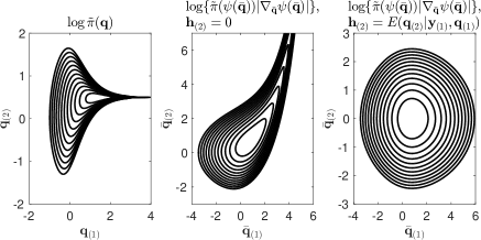
Figure 1: Contour plots of the log-target density associated with (14-16) (left panel) and the associated modified targets based on the scaling matrix $\mathbf{G}(\mathbf{q})=\text{diag}(1+\frac{9}{2},1+\exp(3\mathbf{q}_{(1)}))$ with either $\mathbf{h}_{(2)}=0$ (middle panel) or $\mathbf{h}_{(2)}=E(\mathbf{q}_{(2)}|\mathbf{y}_{(1)},\mathbf{q}_{(1)})$ (right panel). In all cases, $\mathbf{y}_{(1)}=0.5$, and $\mathbf{h}_{(1)}=0$ for both modified targets.

Figure 1 illustrates the effect of going from the original target associated with (14-16) (left panel) to the modified target based on the scaling matrix found above (middle or right panel) for $\mathbf{y}_{(1)}=0.5$. It is seen that for this situation, the original target $\log\tilde{\pi}(\mathbf{q})$ contains substantially different scales depending on the $\mathbf{q}_{(1)}$-coordinate (and thus is problematic for HMC sampling), whereas the modified target has close to constant scaling in both cases, and should therefore be suitable MCMC sampling based on HMC.

4.4 Choosing the location vector $\mathbf{h}_{(r)}$

As is also illustrated by comparing the middle and right panels of Figure 1, the choice of $\mathbf{h}_{(r)},\;r=1,\dots,R$, may influence how well HMC will work on the modified target. The choice $\mathbf{h}_{(2)}=E(\mathbf{q}_{(2)}|\mathbf{y}_{(1)},\mathbf{q}_{(1)})$ in this particular example results in that the modified target distribution that has independent components. On the other hand, finding relevant and sequential dependence-respecting $\mathbf{h}_{(r)}$s, in particular for low-level (small $r$) parameters is difficult. As illustrated in the simulation experiments to be discussed shortly, a rather safe option is to set $\mathbf{h}_{(r)}$ corresponding to low-level parameters equal to zero or alternatively to the marginal expectations of those parameters (obtained from a preliminary run or during warm up).

For more high-level sampled quantities, say e.g. $\mathbf{q}_{(R)}$ (typically a latent field), whose “typical location” conditional on data may move substantially depending on the value of the low-level parameter (in particular in high or variable signal to noise settings such as in Figure 1, left panel), it may be an advantage to set $\mathbf{h}_{(R)}$ equal to some approximation to $E(\mathbf{q}_{(R)}|\mathbf{q}_{(1:R-1)},\mathbf{y}_{(1:S)})$. Assuming here for simplicity that only a single observation block $\mathbf{y}_{(1)}$ depends only on $\mathbf{q}_{(R)}$, a rather generic approach for computing such approximate conditional expectations would be

$$E(\mathbf{q}_{(R)}|\mathbf{q}_{(1:R-1)},\mathbf{y}_{(1)})\approx\mathbf{G}_{(R)}^{-1}(\mathbf{q}_{(1:R-1)})\left[\mathcal{I}_{(R)}^{\mathcal{A}}E(\mathbf{q}_{(R)}|\mathbf{q}_{(1:R-1)})+\mathcal{I}_{(1|R)}^{\mathcal{C}}\hat{\mathbf{q}}_{(R)}\right],\;\hat{\mathbf{q}}_{(R)}=\arg\max_{\mathbf{q}_{(R)}}\log p(\mathbf{y}_{(1)}|\mathbf{q}_{(R)}),$$ (20)

which obtains by approximating $p(\mathbf{q}_{(R)}|\mathbf{q}_{(1:R-1)})$ by $\mathcal{N}(\mathbf{q}_{(R)}|E(\mathbf{q}_{(R)}|\mathbf{q}_{(1:R-1)}),\left[\mathcal{I}_{(R)}^{\mathcal{A}}\right]^{-1})$ and $p(\mathbf{q}_{(R)}|\mathbf{y}_{(1)})$ by $\mathcal{N}(\mathbf{q}_{(R)}|\hat{\mathbf{q}}_{(R)},\left[\mathcal{I}_{(1|R)}^{\mathcal{C}}\right]^{-1})$ and subsequently combining the two sources of Gaussian information. Note that $\mathbf{G}_{(R)}$ in any case must be Cholesky factorised, and therefore this approximation adds only a modest amount of additional computing time. Further, the formula is easily extended to situations with further observation blocks and cases where $\mathbf{q}_{(R)}|\mathbf{q}_{(1:R-1)}$ is improper. Note also that if $\mathbf{q}_{(R)}|\mathbf{q}_{(1:R-1)},\mathbf{y}_{(1:R)}$ indeed is Gaussian, as is the case in the linear/Gaussian state space model and the Stock and Watson model discussed below, the above formula is exact.

4.5 What is lost by disregarding off-diagonal blocks of the Hessian?

A closer look at Figure 1, right panel reveal that of the modified target $\tilde{\pi}(\Psi(\bar{\mathbf{q}}))|\nabla_{\bar{\mathbf{q}}}\Psi(\bar{\mathbf{q}})|$ based on the above found SDBD scaling matrix and $\mathbf{h}_{(2)}=E(\mathbf{q}_{(2)}|\mathbf{y}_{(1)},\mathbf{q}_{(1)})$ does not have unit covariance matrix, but rather $\text{Var}(\bar{\mathbf{q}})\approx\text{diag}(1.9^{2},1)$. This phenomenon is related to fact that the scaling matrix $\mathbf{G}$, for the reasons of computational efficiency detailed above, is chosen to be (block-) diagonal, whereas the negative Hessian, or some relevant SPD approximation to the Hessian, would have non-trivial off-diagonal elements. Thus, a further discussion of the trade-off made by choosing a block-diagonal scaling matrix, and how to make the block-diagonal scaling matrix as good an approximation as possible is in order.

A useful model for studying this phenomena is when the target distribution is a (zero mean) Gaussian with some precision matrix $\mathbf{Q}$ and some blocking $\mathbf{q}_{(1:R)}$. Clearly $p(\mathbf{q})$ can be written as $p(\mathbf{q}_{(1)})p(\mathbf{q}_{(2)}|\mathbf{q}_{(1)})\cdots p(\mathbf{q}_{(R)}|\mathbf{q}_{(1:R-1)}),$ where each of the factors are Gaussian with fixed precision matrices, and the conditioning variables enter only linearly in the mean. Therefore, via the expected negative Hessian representation of the Fisher information, $\mathcal{I}_{(t|r)}^{\mathcal{B}}=\mathcal{B}_{(t|r)},t=2,\dots,R,\;r=1,\dots,t-1,$ and thus $\mathbf{G}_{(r)}$ is equal to the corresponding block of the precision matrix, namely $\mathbf{G}_{(r)}=\text{Prec}(\mathbf{q}_{(r)}|\mathbf{q}_{(-r)})$. Interpreting $\mathbf{G}$ as an inverse covariance matrix leads to the variance representation of $\mathbf{G}$:

$$\mathbf{G}^{-1}=\text{bdiag}(\text{Var}(\mathbf{q}_{(1)}|\mathbf{q}_{(-1)}),\dots,\text{Var}(\mathbf{q}_{(R)}|\mathbf{q}_{(-R)})),\;\text{where }\mathbf{q}_{(-r)}=[\mathbf{q}_{(1:r-1)}^{T},\mathbf{q}_{(r+1:R)}^{T}]^{T}.$$ (21)

Provided the blocks of $\mathbf{q}$ are not independent, working with the block-diagonal $\mathbf{G}$ based on (18) will in this case lead to systematic underestimation of the marginal variances of the original target and consequently, to that the marginal variances being greater than unity under the modified target.

In light of this observation, it is clear that the primary objective of the $\mathbf{G}$-based modification of the target is to remove variable scaling and arrive at approximately fixed (but not necessary unit variance) scaling, as illustrated Figure 1. Fixed, non-unit variance scaling can subsequently be corrected by appropriate choices of the HMC mass matrix $\mathbf{M}$. Still, (21) provide guidance as how to make $\mathbf{G}$ to have as high quality as possible: Firstly, make the blocks as large as possible in order to capture as much of the target dependence structure internally in the blocks. Secondly, use parameterisation of the models so that the cross-block dependence is as weak as possible. In particular, to this end, orthogonal block parameterisations as discussed in Section 4.1 should be used as much as possible.

4.6 Overview of (block-) orthogonal CIPs

This Section gives a brief overview of available CIPs relevant for Bayesian hierarchical models, mainly in order to illustrate that modelling with CIPs constitutes quite a small restriction. More details, including expressions for Fisher informations $\{\mathcal{F}_{r}\}_{r=1}^{p}$ for the mentioned models are available in (non- comprehensive) lists in the supplementary materials, Sections B, C.

For continuous univariate models, Gaussian-, fixed shape Gamma-, Laplace- and Weibull distributions admit closed form orthogonal CIPs, whereas a variable shape Gamma distribution CIPs obtains by solving an implicit equation and is easily approximated numerically. For the $t$-distribution, an approximate orthogonal CIP based on the formulas of Lange et al. (1989) is discussed.

For discrete probability distributions, useful CIPs seem more difficult to come by (e.g. for a Poisson distributed $y$, a CIP obtains when $E(y)=c\theta_{(1)}^{2}$). However, such distributions are by construction only relevant as observation likelihoods in the present framework, and therefore observed Fisher informations are typically used. Supplementary materials, Section B.2 provides observed Fisher informations for Poisson, Binomial and negative Binomial distributions.

With respect to multivariate Gaussian models (which are often used as latent fields) with sampled parameters influencing the mean in a linear manner, both CIPs for unrestricted precision matrices and more structured precision matrices (e.g. stationary AR(1), intrinsic random walk, Besag-type intrinsic GMRFs etc. (see Rue and Held, 2005)) are discussed, and implied Wishart priors under the CIPs for unrestricted precision matrices are given.

5 Simulation experiments

This Section illustrates, benchmarks, and further explores via simulation, different aspects of the proposed methodology for three simple example models. Further details on how to implement DRHMC within Stan are given in supplementary materials, Section D. In the present paper, focus is in particular on time series models as these models only require Cholesky factorisations of tri-diagonal $\mathbf{G}_{(r)}$s. All relevant files for implementing and running the different models can be found at http://www.ux.uis.no/~tore/DRHMC/. See supplementary materials, Section D for more details.

5.1 Linear Gaussian state space model

	Model 1						Model 2
	$\lambda$ Post.	$\lambda$ Post.	$\lambda$ $\hat{n}_{\text{eff}}$	$\mathbf{x}$ $\hat{n}_{\text{eff}}$	CPU		$\tau$ Post.	$\tau$ Post.	$\tau$ $\hat{n}_{\text{eff}}$	$\mathbf{x}$ $\hat{n}_{\text{eff}}$	CPU
	mean	SD		$\geq$	time (s)		mean	SD		$\geq$	time (s)
	Data Set 1 (true $\tau=-\log(0.15^{2})$)
True	4.153	0.290	–	–	–		3.953	0.240	–	–	–
$\mathbf{x}$-prior standardisation	4.152	0.285	3079	10000	1.5		3.948	0.238	4157	10000	2.8
DRHMC, $\mathbf{h}_{(2)}=\mathbf{0}_{T}$	4.151	0.287	7115	10000	1.6		3.954	0.231	747	10000	0.6
DRHMC, $\mathbf{h}_{(2)}=\mathbf{y}$	4.153	0.291	2282	10000	0.6		3.952	0.237	10000	10000	0.5
DRHMC, $\mathbf{h}_{(2)}=E(\mathbf{x}|\mathbf{y},\lambda,\tau$)	4.155	0.292	10000	10000	1.5		3.955	0.242	10000	10000	1.7
RMHMC	4.151	0.293	10000	10000	37		3.928	0.240	10000	10000	35
SSHMC	4.155	0.291	6280	10000	8.4		3.930	0.241	9270	10000	8.4
	Data Set 2 (true $\tau=-\log(0.005^{2})$)
True	3.957	0.142	–	–	–		11.36	2.49	–	–	–
$\mathbf{x}$-prior standardisation	3.965	0.143	130	8707	6.5		9.02	1.57	7	16	4.0
DRHMC, $\mathbf{h}_{(2)}=\mathbf{0}_{T}$	3.958	0.143	10000	10000	1.1		8.08	0.85	9	232	4.5
DRHMC, $\mathbf{h}_{(2)}=\mathbf{y}$	3.957	0.141	10000	10000	1.4		11.39	2.52	10000	6854	1.7
DRHMC, $\mathbf{h}_{(2)}=E(\mathbf{x}|\mathbf{y},\lambda,\tau$)	3.960	0.142	10000	10000	2.2		11.40	2.50	10000	6404	3.1
RMHMC	3.958	0.139	10000	10000	25		7.48	1.02	516	10000	39
SSHMC	3.958	0.142	10000	10000	8.3		7.56	1.08	225	10000	8.4

Table 1: Result from linear Gaussian state space model experiment, models 1 and 2. All figures reported were obtained using RStan and are calculated as the mean over 10 independent replica, with 1000 warmup iterations and 1000 iterations used for collecting samples. “Post. Mean” and “Post. SD.” are posterior mean and standard deviation respectively. $\hat{n}_{\text{eff}}$ is a measure of effective sample size calculated over the independent replica. The column “$\mathbf{x}$ $\hat{n}_{\text{eff}}\geq$” gives the minimum (over $t$) $\hat{n}_{\text{eff}}$ of $\mathbf{x}_{t}$. Reported CPU times are for 1000 iterations. The best parameter effective sample sizes per computing time are indicated with bold font.

	Model 3
	$\lambda$ Post.	$\lambda$ Post.	$\lambda$ $\hat{n}_{\text{eff}}$		$\tau$ Post.	$\tau$ Post.	$\tau$ $\hat{n}_{\text{eff}}$		$\mathbf{x}$ $\hat{n}_{\text{eff}}$	CPU
	mean	SD			mean	SD			$\geq$	time (s)
	Data Set 1 (true $\tau=-\log(0.15^{2})$)
True	4.126	0.337	–		3.808	0.257	–		–	–
$\mathbf{x}$-prior standardisation	4.130	0.334	1461		3.807	0.256	1372		10000	2.1
DRHMC, $\mathbf{h}_{(2)}=\mathbf{0}_{T}$	4.128	0.335	1944		3.807	0.254	782		10000	0.8
DRHMC, $\mathbf{h}_{(2)}=\mathbf{y}$	4.115	0.344	818		3.815	0.266	1786		10000	0.6
DRHMC, $\mathbf{h}_{(2)}=E(\mathbf{x}|\mathbf{y},\lambda,\tau$)	4.127	0.338	8665		3.807	0.258	7211		10000	0.7
RMHMC	4.129	0.337	6529		3.808	0.260	9377		10000	52
SSHMC	4.109	0.343	2880		3.819	0.262	3292		10000	8.4
	Data Set 2 (true $\tau=-\log(0.005^{2})$)
True	4.101	0.194	–		6.867	1.105	–		–	–
$\mathbf{x}$-prior standardisation	3.2e+11	1.1e+12	10		4.983	2.259	5		10000	2.5
DRHMC, $\mathbf{h}_{(2)}=\mathbf{0}_{T}$	4.141	0.195	228		6.329	0.626	18		204	2.9
DRHMC, $\mathbf{h}_{(2)}=\mathbf{y}$	4.103	0.196	5313		6.884	1.156	4624		10000	1.2
DRHMC, $\mathbf{h}_{(2)}=E(\mathbf{x}|\mathbf{y},\lambda,\tau$)	4.098	0.195	10000		6.886	1.131	10000		10000	1.7
RMHMC	4.095	0.193	10000		6.934	1.139	224		10000	55
SSHMC	4.096	0.194	943		6.885	1.088	206		10000	8.4

Table 2: Result from linear Gaussian state space model experiment, model 3. All figures reported were obtained using RStan and are calculated as the mean over 10 independent replica, with 1000 warmup iterations and 1000 iterations used for collecting samples. “Post. Mean” and “Post. SD.” are posterior mean and standard deviation respectively. $\hat{n}_{\text{eff}}$ is a measure of effective sample size calculated over the independent replica. The column “$\mathbf{x}$ $\hat{n}_{\text{eff}}\geq$” gives the minimum (over $t$) $\hat{n}_{\text{eff}}$ of $\mathbf{x}_{t}$. Reported CPU times are for 1000 iterations. The best parameter effective sample sizes per computing time are indicated with bold font.

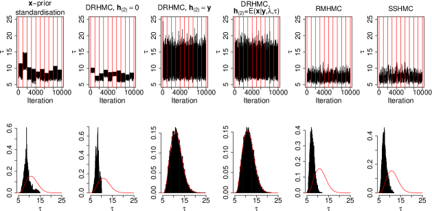
Figure 2: Trace plots and histograms of output for $\tau$ of the linear Gaussian state space model, model 2, applied to Data set 2. The upper panels display trace plots of $\tau$, where samples between two vertical lines correspond to a single replica with 1000 iterations. The lower panels display density-scaled histograms of the combined samples from all ten replica, and the line is the corresponding exact posterior distribution.

The first model used in the simulation study is a linear Gaussian state space model (see e.g. Durbin and Koopman, 2012), where the latent state is a univariate stationary Gaussian AR(1) process. The model allows exact calculation of posterior distributions via the Kalman filter, which can be used as reference for the MCMC results produced. The CIP for a stationary Gaussian AR(1) model obtains by defining $\sigma^{2}(\lambda)=\exp(-\lambda)$ and $\phi(\omega)=\tanh(\psi(\omega))$ where $\psi:\mathbb{R}\mapsto\mathbb{R}$ is discussed in the supplementary materials, Section C.2.1. Then, the parameterisation of the stationary AR(1) process $\{x_{t}\}_{t=1}^{T}$ considered here is

$$x_{1}|\lambda,\omega,\mu \sim N\left(\mu,\frac{\sigma^{2}(\lambda)}{1-\phi(\omega)^{2}}\right)$$ (22)

$$x_{t+1}|x_{t},\lambda,\omega,\mu \sim N(\mu+\phi(\omega)(x_{t}-\mu),\sigma^{2}(\lambda)),\;t=1,\dots,T-1.$$ (23)

The linear Gaussian state space model is further characterised by the observation equation

$$y_{t}|x_{t},\tau\sim N(x_{t},\exp(-\tau)),\;t=1,\dots,T,$$

The mean and autocorrelation parameters were fixed to $\mu=0$ and $\omega=2.2$ (corresponding to $\phi(\omega)\approx 0.9959$ for $T=100$). Three variants of the model are considered;

• Model 1: $\mathbf{q}=(\mathbf{q}_{(1)}=\lambda,\mathbf{q}_{(2)}=\mathbf{x})$, with flat prior on $\lambda$, which leads to $\mathbf{G}=\text{bdiag}(T/2,\text{Prec}(\mathbf{x}|\lambda)+\exp(\tau)\mathbf{I}_{T}$). Here, $\tau$ is fixed at the true value.

• Model 2: $\mathbf{q}=(\mathbf{q}_{(1)}=\tau,\mathbf{q}_{(2)}=\mathbf{x})$, with a $N(0,3^{2})$-prior on $\tau$, which leads to $\mathbf{G}=\text{bdiag}(\frac{1}{9}+\frac{T}{2},\text{Prec}(\mathbf{x}|\lambda)+\exp(\tau)\mathbf{I}_{T})$. Here, $\lambda$ is fixed at the true value.

• Model 3: $\mathbf{q}=(\mathbf{q}_{(1)}=(\lambda,\tau),\mathbf{q}_{(2)}=\mathbf{x})$, with flat prior on $\lambda$ and a $N(0,3^{2})$-prior on $\tau$, which leads to $\mathbf{G}=\text{bdiag}(\text{diag}(\frac{T}{2},\frac{1}{9}+\frac{T}{2}),\text{Prec}(\mathbf{x}|\lambda)+\exp(\tau)\mathbf{I}_{T})$.

All three models were applied to two simulated data sets of length $T=100$. The true parameters were: $\tau=-\log(0.15^{2})$ in data set 1, $\tau=-\log(0.005^{2})$ in data set 2, and $\lambda=-\log(0.15^{2})$ for both data sets. The models and true parameters of the data sets are chosen to highlight different aspects of the proposed methodology.

DRHMC-methods based on the above presented scaling matrices were implemented using three alternative second block location vectors, namely $\mathbf{h}_{(2)}=\mathbf{0}_{T},\,\mathbf{h}_{(2)}=\mathbf{y}$ and $\mathbf{h}_{(2)}=E(\mathbf{x}|\mathbf{y},\lambda,\tau)$, where the latter has closed form due to the linear and Gaussian structure of the model. Note that for $\mathbf{h}_{(2)}=E(\mathbf{x}|\mathbf{y},\lambda,\tau)$, $\mathbf{\bar{q}}_{(1)}$ and $\mathbf{\bar{q}}_{(2)}$ are independent, and $\mathbf{\bar{q}}_{(2)}$ is standard Gaussian under the modified target. As benchmarks, the following methods were considered:

• $\mathbf{x}$-prior standardisation: direct application of Stan HMC to parameter(s) and the standardised residuals of $\mathbf{x}$ (i.e. $\mathbf{z}$ where $\mathbf{z}_{1}=\mathbf{x}_{1}\exp(\lambda/2)\sqrt{1-\phi^{2}}$, $\mathbf{z}_{t}=(\mathbf{x}_{t}-\phi\mathbf{x}_{t-1})\exp(\lambda/2),\;t=2,\dots,T$).

• RMHMC: the modified Cholesky RMHMC of Kleppe (2018), see supplementary materials, Section E.1 for details.

• SSHMC: the semi-separable HMC of Zhang and Sutton (2014), see supplementary materials, Section E.2 for details.

The results are presented in Table 1 for model 1 and 2, and in Table 2 for model 3. All computations presented in this paper were implemented in R (R Core Team, 2017) and RStan (Stan Development Team, 2017a, Version 2.17.4) and run on a 2014 Macbook Pro. Unless otherwise noted, default parameters in (R-functions) stan()/sampling() were used. For each combination of method, model and data set, 10 independent chains were run, with 1000 warm-up iterations, and the subsequent 1000 iterations recorded. The reported $\hat{n}_{\text{eff}}$ is a measure of effective sample size (See Gelman et al., 2014, Chapter 11.5) computed across the different independent chains, whereas reported computing times are for the generation of 1000 samples. The same method for calculating $\hat{n}_{\text{eff}}$ (R-function rstan::monitor()) was also applied for the non-Stan methods RMHMC and SSHMC.

From Tables 1 and 2 it is first seen that due to the exact independence of all sampled quantities for DRHMC, $\mathbf{h}_{(2)}=E(\mathbf{x}|\mathbf{y},\lambda,\tau)$, perfect or close to perfect $\hat{n}_{\text{eff}}$ is obtained for each setting of the experiment. Secondly, $\mathbf{x}$-prior standardisation fares quite well for the low signal-to-noise data set 1 whereas the performance is poor for the high signal-to-noise data set 2. This follows from that for data set 2, the vast majority of information w.r.t. $\mathbf{x}$ comes from the observations, and thus the prior-based standardisation relation between $\mathbf{z}$ and $\mathbf{x}$ is irrelevant for this target. The choice of $\mathbf{h}_{(2)}$ is also seen to a varying degree to impact the performance. In particular when the observation noise precision $\tau$ is sampled in model 2, $\mathbf{h}_{(2)}=\mathbf{y}$ and $\mathbf{h}_{(2)}=E(\mathbf{x}|\mathbf{y},\lambda,\tau)$ produces substantially better performance than for $\mathbf{h}_{(2)}=\mathbf{0}_{T}$. For model 3, $\mathbf{h}_{(2)}=E(\mathbf{x}|\mathbf{y},\lambda,\tau)$ fares substantially better than $\mathbf{h}_{(2)}=\mathbf{y}$. The results indicates that a rule of thumb would be that for a non-linear model where exact conditional expectations are unavailable, extra care must be taken when choosing the $\mathbf{h}_{(r)}$s corresponding to latent fields, in particular in the cases where scales of either the prior or the observation information changes substantially across the target distribution. Comparing DRHMC with the other benchmarks RMHMC and SSHMC, it is seen that the DRHMC methods produces effective samples at a much higher rate. Moreover, for RMHMC and SSHMC, a competitive tuning that properly explores the target for dataset 2 when $\tau$ is sampled (models 2,3) could not be found.

Figure 2 displays trace plots and histograms (with true posterior marginal density as reference) for $\tau$ in the model 2, data set 2 case. This case is characterised by a large variance in $\tau$, and thus substantial variation of the scale of $\mathbf{x}$. In the cases of $\mathbf{x}$-prior standardisation and DRHMC, $\mathbf{h}_{(2)}=\mathbf{0}_{T}$, the different independent chains stabilises in different parts of the target distribution and lead to poor effective sample sizes. Such behaviour is typically seen for target distributions with a strong “funnel”-nature when applying automatic tuning of the HMC sampler parameters is applied. I.e., the automatic tuning typically adapts to different regions of the target with different scaling properties. On the other hand, the plots suggest that the proposed modified parameterisation with either $\mathbf{h}_{(2)}=\mathbf{y}$ or $\mathbf{h}_{(2)}=E(\mathbf{x}|\mathbf{y},\lambda,\tau)$ result in a well-behaved modified target distribution where the automatic tuning of the HMC sampler is very robust. For RMHMC, a selection of the regularisation parameter that lead to converging implicit leap frog steps and at the same time proper exploration of the target distribution could not be found. For SSHMC, it appears that the asynchronous updating of parameters and latent variables inhibits the exploration of the complete target.

5.2 Stochastic volatility model

Block	$\mathcal{I}^{\mathcal{A}}$	$\mathcal{I}^{\mathcal{B}}$	$\mathcal{I}^{\mathcal{C}}$
$\mathbf{q}_{(1)}=\lambda$	$5.0$	$\frac{T}{2}$	–
$\mathbf{q}_{(2)}=\omega$	$\xi(T)$	$\frac{T}{2}$	–
$\mathbf{q}_{(3)}=\mu$	$\frac{1}{100}$	$\exp(\lambda)\left[2(T-1)(1-\phi(\omega))-\frac{T-2}{\cosh(\psi(\omega))^{2}}\right]$	–
$\mathbf{q}_{(4)}=\mathbf{x}=\{x_{t}\}_{t=1}^{T}$	$\text{Prec}(\mathbf{x}|\lambda,\omega)$	–	$\frac{1}{2}\mathbf{I}_{T}$

Table 3: Blocking and terms in the scaling matrix diagonal blocks (18) for the stochastic volatility model. $\xi(T)$ is the Laplace-based approximate precision of the prior on $\omega$ implied by (24). Matrix $\text{Prec}(\mathbf{x}|\lambda,\omega)$ is the tridiagonal precision matrix associated with the AR(1) process. Note in particular that $\mathbf{G}_{(4)}=\text{Prec}(\mathbf{x}|\lambda,\omega)+\frac{1}{2}\mathbf{I}_{T}$ is also tridiagonal.

	$\sigma$	$\phi$	$\mu$	$x_{1}$	$x_{T}$	$x_{t},\;t=1,\dots,T$
$\mathbf{x}$-prior parameterisation, mean CPU time$=50$ seconds
Post. Mean	0.120	0.992	0.103	0.514	-0.129	–
Post. SD.	0.013	0.003	0.367	0.396	0.413	–
$\hat{n}_{\text{eff}}$	4344	4147	4739	10000	10000	$\geq$10000
DRHMC, $\mathbf{h}_{(4)}=\mathbf{0}_{T}$, mean CPU time $=32$ seconds
Post. Mean	0.120	0.993	0.102	0.517	-0.133
Post. SD.	0.013	0.003	0.414	0.397	0.411
$\hat{n}_{\text{eff}}$	9007	10000	10000	10000	10000	$\geq$10000
DRHMC, $\mathbf{h}_{(4)}=\mu\mathbf{1}_{T}$, mean CPU time $=72$ seconds
Post. Mean	0.120	0.993	0.130	0.520	-0.129
Post. SD.	0.012	0.003	0.361	0.398	0.401
$\hat{n}_{\text{eff}}$	4896	516	256	10000	10000	$\geq$10000
DRHMC, $\mathbf{h}_{(4)}=\mathbf{G}_{(4)}^{-1}(\mu\text{Prec}(\mathbf{x}|\lambda,\omega,\mu)\mathbf{1}_{T}+\frac{1}{2}\hat{\mathbf{x}}),$ $\hat{\mathbf{x}}_{i}=\log(\mathbf{y}_{i}^{2})$,
mean CPU time $=47$ seconds.
Post. Mean	0.120	0.993	0.098	0.518	-0.131
Post. SD.	0.012	0.003	0.405	0.394	0.401
$\hat{n}_{\text{eff}}$	8700	10000	10000	10000	10000	$\geq$10000

Table 4: Results for the stochastic volatility model example. All figures reported were obtained using RStan and are calculated as the mean over 10 independent replica, with 1000 warmup iterations and 1000 iterations used for collecting samples. “Post. Mean” and “Post. SD.” are posterior mean and standard deviation respectively. $\hat{n}_{\text{eff}}$ is a measure of effective sample size calculated over the independent replica, and the last column gives the minimum (over $t$) $\hat{n}_{\text{eff}}$ of $x_{t}$. CPU times are for 1000 iterations. The best effective sample sizes per computing time are indicated with bold font.

The second simulation experiment involves a basic stochastic volatility model (see e.g. Kim et al., 1998; Shephard, 2005) where observations are modelled as

$$y_{t}|x_{t}\sim N(0,\exp(x_{t})),\;t=1,\dots,T,$$

and $\{x_{t}\}_{t=1}^{T}|\lambda,\omega,\mu$ is distributed according to (22,23). The model is finalised by the standard priors (see e.g. Kim et al., 1998):

$$\exp(\lambda) \sim\text{Gamma}(5,0.05),$$

$$\frac{1}{2}\left(\phi(\omega)+1\right) \sim\text{Beta}(20,1.5),$$ (24)

$$\mu \sim N(0,10^{2}).$$

The blocking of sampled quantities and terms in the scaling matrix diagonal blocks used for DRHMC are detailed in Table 3. Three variants of DRHMC were considered, with $\mathbf{h}_{(4)}=\mathbf{0}_{T}$, $\mathbf{h}_{(4)}=\mu\mathbf{1}_{T}$ and $\mathbf{h}_{(4)}=\mathbf{G}_{(4)}^{-1}(\mathcal{I}_{(4)}^{\mathcal{A}}(\mu\mathbf{1}_{T})+\mathcal{I}_{(1|4)}^{\mathcal{C}}\hat{\mathbf{x}})$ $=\mathbf{G}_{(4)}^{-1}(\mu\text{Prec}(\mathbf{x}|\lambda,\omega,\mu)\mathbf{1}_{T}+\frac{1}{2}\hat{\mathbf{x}})$ where $\hat{\mathbf{x}}_{t}=\log(\mathbf{y}_{t}^{2}),\;t=1,\dots,T$. The latter may be regarded as an approximation to $E(\mathbf{x}|\mathbf{y},\lambda,\omega,\mu)$ and obtains from (20). A reference procedure, denoted as “$\mathbf{x}$-prior standardisation”, is similar as for the linear Gaussian state space model described above, where the standardised $N(0,1)$ innovations of the $\mathbf{x}$-process are regarded as the latent variables, and non-CIP parameterisation of the first order autoregressive parameter was applied. All methods were implemented in RStan, with some additional C++ code for computing $\psi(\omega)$ and a second order derivative-based approximation $\xi(T)$ to the prior precision of $\omega$ implied by (24). For DRHMC, the maximum tree depth was set to 6, and otherwise default settings were used. The data set was $T=2515$ daily log-return$\times 100$ observations of S&P500 between October 1st, 1999 and September 30th, 2009, previously used by Grothe et al. (2016).

Table 4 provides results and it is seen from the simulation experiment that DRHMC with $\mathbf{h}_{(4)}=\mathbf{0}_{T}$ and $\mathbf{h}_{(4)}\approx E(\mathbf{x}|\mathbf{y},\lambda,\omega,\mu)$ produces close to iid chains for all of the parameters, with the latter requiring slightly higher computing times. In particular, DRHMC with $\mathbf{h}_{(4)}=\mathbf{0}_{T}$ produces a speed up of sampling parameters by roughly a factor 3 relative to the reference. On the other hand, DRHMC with $\mathbf{h}_{(4)}=\mu\mathbf{1}_{T}$ performs substantially poorer than the reference, and thus it is seen that a poor, non-fixed, guess for $\mathbf{h}$ can indeed lead to worse performance than the reference. For all methods, perfect effective sample sizes are obtained for the latent variables. The model involves rather un-informative observations, and the information conveyed by the observations does not vary with any parameter. Therefore, the above, modest improvements over the reference are as expected.

5.3 Crossed random effects - the Salamander mating data

	Default				Standardised				Full CIP/
	implementation,				random effects,				DRHMC,
	mean CPU time $=7.4$ s				mean CPU time $=3.9$ s				mean CPU time $=2.9$ s
	Post.	Post.	$\hat{n}_{\text{eff}}$		Post.	Post.	$\hat{n}_{\text{eff}}$		Post.	Post.	$\hat{n}_{\text{eff}}$
	mean	SD			mean	SD			mean	SD
$\text{Prec}(\mathbf{b}_{i1}^{F})$	1.13	0.9	1828		1.12	0.9	5356		1.10	0.9	4898
$\text{Prec}(\mathbf{b}_{i2}^{F})$	0.92	0.7	2553		0.92	0.8	4531		0.92	0.8	4776
$\text{Corr}(\mathbf{b}_{i1}^{F},\mathbf{b}_{i2}^{F})$	-0.09	0.4	2214		-0.07	0.4	2258		-0.09	0.4	1989
$\text{Prec}(\mathbf{b}_{j1}^{M})$	1.53	1.2	2260		1.54	1.2	4216		1.51	1.2	4468
$\text{Prec}(\mathbf{b}_{j2}^{M})$	1.12	0.9	2033		1.10	0.8	4487		1.07	0.8	4886
$\text{Corr}(\mathbf{b}_{i1}^{M},\mathbf{b}_{i2}^{M})$	0.63	0.3	2093		0.63	0.3	2501		0.64	0.3	2855
$\tau_{F}$	2.21	1.6	2167		2.19	1.6	7381		2.20	1.5	6639
$\tau_{M}$	0.74	0.6	2044		0.72	0.6	4222		0.71	0.5	5095
Random effects	–	–	$\geq$3104		–	–	$\geq$5293		–	–	$\geq$5009
Fixed effects	–	–	$\geq$3268		–	–	$\geq$4008		–	–	$\geq$3602

Table 5: Results for the Salamander mating model. Marginal precisions $\text{Prec}(\mathbf{b}_{i1})$, $\text{Prec}(\mathbf{b}_{i2})$ and correlation $\text{Corr}(\mathbf{b}_{i1},\mathbf{b}_{i2})$ are calculated from samples of $\mathbf{P}$ under the posterior distribution. Posterior mean and SD were obtained as the mean over 10 independent replica with 1000 iterations (and 1000 warm up iterations). The effective sample sizes $\hat{n}_{\text{eff}}$ are calculated across all 10 replica, whereas the CPU times are averages for producing 1000 iterations. The best effective sample sizes per computing time are indicated with bold font. For the random effects ($\text{$\mathbf{b}$}_{ik}^{F}$, $\mathbf{b}_{jk}^{M}$) and fixed effects ($\beta_{l}$), only the minimum (over effect) $\hat{n}_{\text{eff}}$ is reported.

This Section considers a crossed random effects model with binary outcomes for the Salamander mating data described in detail in McCullagh and Nelder (1989, Chapter 14.5). The model considered is identical to the INLA example model “Salamander model B” obtained from
http://www.r-inla.org/examples/volume-ii, and is characterised by

$$\tau_{F} \sim\text{Gamma}(1,0.622),\;\tau_{M}\sim\text{Gamma}(1,0.622)$$

$$\mathbf{P}_{F} \sim\text{Wishart}_{2}(3.0,\mathbf{\mathbf{W}}),\;\mathbf{P}_{M}\sim\text{Wishart}_{2}(3.0,\mathbf{\mathbf{W}}),\;\mathbf{W}=\text{diag}(0.804,0.804),$$

$$\left(\begin{array}[]{c}\mathbf{b}_{i1}^{F}\\ \mathbf{b}_{i2}^{F}\end{array}\right) \sim\text{iid }N(\mathbf{0}_{2},\mathbf{P}_{F}^{-1})\;i=1,\dots,20,\;\left(\begin{array}[]{c}\mathbf{b}_{j1}^{M}\\ \mathbf{b}_{j2}^{M}\end{array}\right)\sim\text{iid }N(\mathbf{0}_{2},\mathbf{P}_{M}^{-1}),\;j=1,\dots,20,$$

$$\mathbf{b}_{i3}^{F} \sim\text{iid }N(0,\tau_{F}^{-1}),\;i=1,\dots,20,\;\mathbf{b}_{j3}^{M}\sim\text{iid }N(0,\tau_{M}^{-1}),\;j=1,\dots,20,$$

$$\mathbf{y}_{ijk}|\pi_{ijk} \sim\text{Binomial}(1,\pi_{ijk}),\;\text{logit}(\pi_{ijk})=\text{$\mathbf{x}$}_{ijk}^{T}\beta+\mathbf{b}_{ik}^{F}+\mathbf{b}_{jk}^{M}.$$

Here $\mathbf{b}_{ik}^{F}$ ($\mathbf{b}_{jk}^{M}$) are random effects specific to female (male) $i$ ($j$) in experiment $k=1,2,3$. The salamanders of experiment 1 and 2 are identical, and therefore the individual specific random effects are allowed to be correlated. Successful mating was recorded as $\mathbf{y}_{ijk}=1$ for 360 combinations of female salamander $i$ and male salamander $j$ in experiment $k$. Here $\mathbf{x}_{ijk}\in\mathbb{R}^{5}$ is covariate vector (including an intercept) and $\mathbf{\beta}\in\mathbb{R}^{5}$ a fixed effect with flat prior.

Due to the low, and fixed with respect to parameters, information content in the observations $\mathbf{y}_{ijk}$, the $\mathcal{C}$-information for this model is fixed to zero. I.e. treating each individual observation as one block leads to zero observed Fisher information (supplementary materials, Table 9) and treating all observations as a single block leads to an un-identified optimiser of $\log p(\mathbf{y}_{ijk}|\beta,\mathbf{b}_{ik}^{F},\mathbf{b}_{jk}^{M})$ w.r.t. $\beta,\mathbf{b}_{ik}^{F},\mathbf{b}_{jk}^{M}$. Thus this simulation experiment focusses primarily on 1) the effect of using standard Gaussian variates as modified parameters for the random effects, (i.e. $\mathbf{b}_{i3}^{F}=\bar{\mathbf{b}_{i3}^{F}}\tau_{F}^{-\frac{1}{2}}$ and so on, which obtains using the methodology explained above with $\mathcal{I}^{\mathcal{C}}=0$), and 2) the effect of using the block-orthogonal CIP of the precision matrix $\mathbf{P}$ for a bivariate Gaussian:

$$\mathbf{P}=\left[\begin{array}[]{cc}\exp(\lambda_{1})&V^{[1]}\exp(\lambda_{1})\\ V^{[1]}\exp(\lambda_{1})&\exp(\lambda_{2})+(V^{[1]})^{2}\exp(\lambda_{1})\end{array}\right],\;\theta_{(1)}=\lambda\in\mathbb{R}^{2},\;\theta_{(2)}=\mathbf{V}^{[1]}\in\mathbb{R},$$

for precision matrices $\mathbf{P}_{F}$,$\mathbf{P}_{M}$, relative to the (different) parameterisation of SPD data type cov_matrix and Wishart distributions used internally in Stan (See Stan Development Team, 2017b, Section 35.9). See supplementary materials, Section C.1, for a CIP of precision matrices of arbitrary order, and also associated Fisher information and implied Wishart distribution. Results for a default implementation (sampled parameters $(\mathbf{\beta},\mathbf{b}_{ik}^{F},\mathbf{b}_{jk}^{M},\mathbf{P}_{F},\mathbf{P}_{M},\mathbf{\tau}_{F},\tau_{M}))$, standardised random effects (sampled parameters $(\mathbf{\beta},\bar{\mathbf{b}_{ik}^{F}},\bar{\mathbf{b}_{jk}^{M}},\mathbf{P}_{F},\mathbf{P}_{M},\mathbf{\tau}_{F},\tau_{M})$, similar to $\mathbf{x}$-prior standardisation discussed above) and a fully CIP/DRHMC implementation (sampled parameters $(\mathbf{\beta},\bar{\mathbf{b}_{ik}^{F}},\bar{\mathbf{b}_{jk}^{M}},\bar{\lambda_{F}},\bar{\mathbf{V}_{F}^{[1]}},\bar{\lambda_{M}},\bar{\mathbf{V}_{M}^{[1]}},\bar{\log\mathbf{\tau}_{F}},\bar{\log\tau_{M}})$, all location vectors $\mathbf{h}_{(r)}$ are fixed to zero) are presented in Table 5.

Table 5 focuses mainly on the more difficult parameters, namely the random effects variance structure. The effective samples sizes of the random- and fixed effects are fairly good in all cases. It is seen that choosing a standardised random effects parameterisation is beneficial relative to the default implementation both in terms of CPU time and effective sample size, but the effect is not very large as the variance of random effects parameters have quite tight priors. Moreover, it is seen that introducing the CIP parameterisation of the precision matrices seems to further improve sampling efficiency, but again the gains are not very large for this particular model.

6 Realistic application - the Stock and Watson (2007) model

Block	$\mathcal{I}^{\mathcal{A}}$	$\mathcal{I}^{\mathcal{B}}$	$\mathcal{I}^{\mathcal{C}}$
$\mathbf{q}_{(1)}=\lambda$	$5.0$	$\frac{T-1}{2}+\frac{T-2}{2}$	–
$\mathbf{q}_{(2)}=\mathbf{z}=\{z_{t}\}_{t=1}^{T-1}$	$\text{Prec}(\mathbf{z}|\lambda)$	$\frac{1}{2}\mathbf{I}_{T-1}$	–
$\mathbf{q}_{(3)}=\mathbf{x}=\{x_{t}\}_{t=1}^{T}$	$\text{Prec}(\mathbf{x}|\lambda)$	–	$\frac{1}{2}\mathbf{I}_{T}$
$\mathbf{q}_{(4)}=\mathbf{\tau}=\{\tau_{t}\}_{t=1}^{T}$	$\text{Prec}(\mathbf{\tau}|\mathbf{z})$	–	$\mathbf{P}_{\mathbf{y}}(\mathbf{x})=\text{diag}(\exp(-x_{1}),\dots,\exp(-x_{T}))$

Table 6: Blocking and information matrices for the Stock and Watson (2007) model (25-28). Note that the precision matrices $\text{Prec}(\mathbf{z}|\lambda)$, $\text{Prec}(\mathbf{x}|\lambda)$ and $\text{Prec}(\mathbf{\tau}|\mathbf{z})$ are degenerate, but the resulting scaling matrix diagonal blocks are all SPD. The prior approximate precision of $\lambda$ obtains via a second order derivative-based approximation of the logarithm of Gamma, which in general yields that $\mathcal{I}^{\mathcal{A}}$ should be set equal to the shape parameter.

	DRHMC, Method 0,				DRHMC, Method 1,				Direct HMC,
	mean CPU time $=9.1$ s				mean CPU time $=30.5$ s				mean CPU time $=87.6$ s
	Post.	Post.	$\hat{n}_{\text{eff}}$		Post.	Post.	$\hat{n}_{\text{eff}}$		Post.	Post.	$\hat{n}_{\text{eff}}$
	mean	SD			mean	SD			mean	SD
$\lambda$	2.35	0.3	2568		2.34	0.3	3804		2.33	0.3	230
$z_{1}$	-4.94	1.9	1462		-5.02	1.9	1719		-4.65	1.8	248
$z_{t}$	–	–	$\geq$624		–	–	$\geq$1324		–	–	$\geq$39
$x_{1}$	-1.71	0.8	5551		-1.72	0.8	10000		-1.77	0.8	1377
$x_{t}$	–	–	$\geq$1561		–	–	$\geq$2180		–	–	$\geq$208
$\tau_{1}$	0.35	0.2	5695		0.35	0.2	10000		0.33	0.2	1132
$\tau_{t}$	–	–	$\geq$2039		–	–	$\geq$2928		–	–	$\geq$114
$\bar{\lambda}$	37.5	4.7	2568		0.0	0.95	3804		–	–	–
$\bar{z}_{1}$	-0.76	1.1	10000		-0.1	1.06	10000		–	–	–
$\bar{x}_{1}$	-0.26	1.0	10000		0.0	1.02	10000		–	–	–
$\bar{\tau}_{1}$	0.0	1.0	10000		0.0	1.02	10000		–	–	–

Table 7: Results for the Stock and Watson (2007) model (25-28) applied to US inflation data between Q1-1955 and Q1-2018. DRHMC, Method 0 correspond to direct application of the proposed methodology where $\mathbf{h}_{(1)},\mathbf{h}_{(2)},\text{$\mathbf{h}$}_{(3)}$ are set to zero, whereas in DRHMC, Method 1, a preliminary run of method 0 is used to find fixed values for $\mathbf{h}_{(1)},\mathbf{h}_{(2)},\text{$\mathbf{h}$}_{(3)}$ and also $\mathbf{G}_{(1)}$. Direct HMC uses the default parameterisation of (25-28). All results are based on 10 independent chains, each with 1000 iterations and 1000 warm up iterations. The effective sample sizes ($\hat{n}_{\text{eff}}$) are calculated across the combined iterations, whereas CPU times are for 1000 iterations. The rows $z_{t}$, $x_{t}$ and $\tau_{t}$ give the minimum (over $t$) $\hat{n}_{\text{eff}}$. The best effective sample sizes per computing time are indicated in bold font.

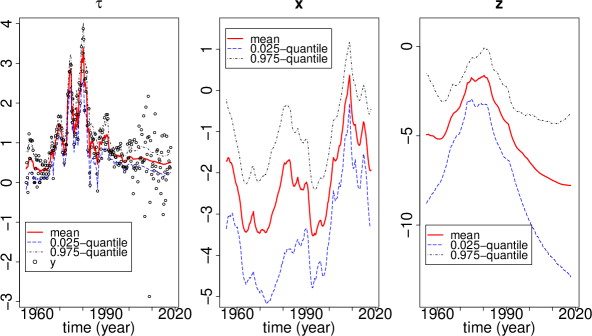
Figure 3: Posterior distributions of the latent processes for the Stock and Watson (2007) model (25-28) applied to US inflation data between Q1-1955 and Q1-2018 based on DRHMC, Method 0. The left panel depicts (marginal) posterior mean, 0.025- and 0.975-quantiles for the $\tau$-process. Actual observations $\mathbf{y}$ are indicated with circles. The middle and right panels depict (marginal) posterior mean, 0.025- and 0.975-quantiles for the $\mathbf{x}$ and $\mathbf{z}$ processes respectively.

The realistic model used for illustrating the proposed methodology is the Stock and Watson (2007) model for observed inflation rates $\mathbf{y}=\{y_{t}\}_{t=1}^{T}$, which may be written as:

$$y_{t}|\tau_{t},x_{t} \sim N(\tau_{t},\exp(x_{t})),\;t=1,\dots,T,$$ (25)

$$\tau_{t}|\tau_{t-1},z_{t-1} \sim N(\tau_{t-1},\exp(z_{t-1})),\;t=2,\dots,T,$$ (26)

$$x_{t}|x_{t-1},\lambda \sim N(x_{t-1},\exp(-\lambda)),\;t=2,\dots,T,$$ (27)

$$z_{t}|z_{t-1},\lambda \sim N(z_{t-1},\exp(-\lambda)),\;t=2,\dots,T-1,$$ (28)

and completed with prior $\exp(\lambda)\sim\text{Gamma}(5,0.5)$. Here, $\mathbf{\tau}=\{\tau_{t}\}_{t=1}^{T}$ is a latent first order random walk stochastic trend component, and both $\mathbf{y}$ and $\mathbf{\tau}$ are subject to stochastic volatility driven by $\mathbf{x}=\{x_{t}\}_{t=1}^{T}$ and $\mathbf{z}=\{z_{t}\}_{t=1}^{T-1}$ respectively. Note that $\mathbf{z}|\lambda$, $\mathbf{x}|\lambda$ and $\mathbf{\tau}|\mathbf{z}$ are all intrinsic Gaussian first order random walk processes, and that the model has “two levels” ($(\mathbf{z},\mathbf{x})$ and $\tau$) of latent variables, which have a strongly non-linear joint distribution. I.e. $p(\mathbf{x},\mathbf{z},\lambda)$, $p(\mathbf{\tau},\mathbf{z}|\lambda)$ and $p(\mathbf{\tau},\mathbf{x}|\mathbf{y},\lambda)$ all have high-dimensional “funnel”-like structure. Such a model would in particular be challenging for methods based on the Laplace approximation such as INLA (Rue et al., 2009), and recently, specialised computational methods for such models have been developed (see e.g. Moura and Turatti, 2014; Shephard, 2015; Li and Koopman, 2018). Here, on the other hand, it is shown that with a very modest coding effort under the proposed methodology, this model is easily tackled using the general purpose Stan software.

Blocking and related information is presented in Table 6. Two variants of DRHMC were considered. The former, referred to as Method 0, is based on $\mathbf{h}_{(1)}=0,\;\mathbf{h}_{(2)}=\mathbf{0}_{T-1},\;\mathbf{h}_{(3)}=\mathbf{0}_{T}$ in line with the finds in Section 5.2 and due to lack of obvious sequentially dependent choices for $\mathbf{h}_{(1)},\mathbf{h}_{(2)},\mathbf{h}_{(3)}$. In Method 1, a preliminary chain using Method 0 is first run, and subsequently $\mathbf{h}_{(1)},\mathbf{h}_{(2)},\mathbf{h}_{(3)}$ are set to the estimated posterior mean of $\lambda$, $\mathbf{z}$ and $\mathbf{x}$ respectively. Moreover, in Method $1$, the $\lambda$ scaling matrix $\mathbf{G}_{(1)}$ is set equal to the estimate of the marginal posterior precision of $\lambda$ from the preliminary run, and for this method the HMC scaling matrix $\mathbf{M}$ is set equal to identity. In both methods, $\mathbf{h}_{(4)}=E(\mathbf{\tau}|\mathbf{z},\mathbf{x},\mathbf{y},\lambda)=\mathbf{G}_{(4)}^{-1}(\mathbf{x},\mathbf{z})\mathbf{P}_{\mathbf{y}}(\mathbf{x})\mathbf{y}$ (as $\mathbf{\tau}|\mathbf{z},\mathbf{x},\mathbf{y},\lambda$ has a proper Gaussian distribution), and this choice effectively integrates out $\mathbf{\tau}$ from the target.

Direct HMC sampling (i.e. parameterisation $(\lambda,\mathbf{z},\mathbf{x},\mathbf{\tau})$ as the intrinsic priors on $\mathbf{z}$, $\mathbf{x}$ and $\tau$ does not admit straight forward prior standardisation) implemented in RStan is used as a reference. The data $\mathbf{y}$ consist of $T=252$ log-return$\times 100$ observations of quarterly US CPI between first quarter of 1955 and first quarter 2018, obtained from the OECD statistics web site http://stats.oecd.org.

Results, comparing the three methods, are presented in Table 7, and Figure 3 gives a representation of the posterior distribution of the latent processes. From the Table, it is seen that direct HMC for this model works very poorly, even when tuned towards an acceptance rate of 0.99. This observation is also corroborated by the facts that several proposals resulted in divergent simulation of the dynamics, and that most of the transitions involve exhausting the default allowed number of leap frog steps. In tandem, these observations indicate that the scaling properties of the target (in $(\lambda,\mathbf{z},\mathbf{x},\mathbf{\tau})$) are too variable for a globally tuned HMC.

The two DRHMC methods produce robust results. It is seen that DRHMC, Method 0 produces consistently the best effective sample sizes per computing time, in large part because of the very fast computing times. Notice that, due to the numerical linear algebra involved in computing the modified target, the per leap frog step computational cost of say DRHMC, method 0 is substantially higher than that of direct HMC (0.36 s vs 0.096 s per 1000 steps). Still, this effect is more than out-weighted by the substantially fewer leap frog steps per proposal that are required for DRHMC, method 0 relative to direct HMC (on average, 25 vs 915 steps per proposal).

Looking at the distributions for the modified parameterisation, it is seen that for both DRHMC methods, the modified latent variables are close to standardised (this is indeed the case for all periods, but only first period is presented in the Table), whereas the standardisation of $\lambda$ under method 0 is somewhat inaccurate due to dependencies not captured by the block-diagonal scaling matrix.

From Figure 3, it is seen that the data suggest both substantial time-variation in both the signal-to-noise ratio and volatility of the latent process $\tau$ across the support of the target distribution, where both of the features gives rise to “funnel”-like structures. Still, by accounting for these effects through the scaling matrix enables the usage HMC as in a very effective manner.

7 Discussion

This paper has discussed the dynamically rescaled Hamiltonian Monte Carlo method as a computationally fast way of performing full Bayesian analysis of non-linear/non-Gaussian Bayesian hierarchical models. Through simulation experiments, the methodology has been shown to be highly competitive, while retaining that the methodology is easily implemented in Stan (or some other high level MCMC software). Several extensions/modifications to the methodology has been kept out of the paper, both in the interest of keeping the paper at a manageable length, but also as they are more difficult, though by no means impossible, to implement in Stan.

The former such extension would be to consider latent models which gives rise to more complicated sparsity pattern for high-dimensional $\mathbf{G}_{(r)}$s, such as e.g. when $\mathbf{q}_{(r)}$ is a priori a spatial or spatial-temporal Gaussian Markov random field. The current version of Stan does not implement a sparse Cholesky factorisation (see e.g. Davis, 2006) within its automatic differentiation framework. However, such routines will be available in Stan in the future and thus DRHMC for spatial models will be straightforward to implement then.

A second extension is particularly relevant for a non-linear/non-Gaussian latent model, say $\mathbf{q}_{(R)}$, where the precision matrix $\mathcal{I}_{R}^{\mathcal{A}}$ is either unavailable or poorly reflect the local scaling properties of $\mathbf{q}_{(R)}$ (e.g. dynamic models where transition variance depend on current position). In this case, sequential dependence-respecting location and scale information adapted to observations may be obtained using a Laplace approximation approach, i.e. (assuming for simplicity that all observations are collected in a single block $\mathbf{y}_{(1)}$)

$$\mathbf{h}_{(R)}(\mathbf{q}_{(1:R-1)}) =\arg\max_{\mathbf{q}_{(R)}}\log\left[p(\mathbf{q}_{(R)}|\mathbf{q}_{(1:R-1)})p(\mathbf{y}_{(1)}|\mathbf{q}_{(1:R)})\right],$$ (29)

$$\mathbf{G}_{(R)}(\mathbf{q}_{(1:R-1)}) =-\nabla_{\mathbf{q}_{(R)},\mathbf{q}_{(R)}}^{2}\log\left[p(\mathbf{q}_{(R)}|\mathbf{q}_{(1:R-1)})p(\mathbf{y}_{(1)}|\mathbf{q}_{(1:R)})\right]|_{\mathbf{q}_{(R)}=\mathbf{h}_{(R)}(\mathbf{q}_{(1:R-1)})}.$$ (30)

Such an implementation would require an “inner” optimisation step (29) for each evaluation of the modified target, which is somewhat more challenging to implement in Stan. However, as demonstrated by INLA and TMB, which both compute substantial numbers of such inner optimisers during a model fitting process, DRHMC with inner optimisation steps should be possible and may produce substantial speed-ups in certain situations. Note that applying the Laplace approximation location vector (29) and precision matrix (30) effectively makes DRHMC a pseudo-marginal method (Andrieu et al., 2010) where the modified target involves a Laplace approximation to the marginal parameter posterior (and being exact in conditionally linear Gaussian cases such as in Sections 5.1,6). However, the mechanism for correcting for such approximation error under DRHMC is very different from methods relying on unbiased Monte Carlo estimates such as particle MCMC (Andrieu et al., 2010) or even pseudo-marginal HMC (Lindsten and Doucet, 2016). Assessing the merits and limitations of such a Laplace approximation-based approach is currently on the research agenda. The approach may benefit from applying the more specialised integrator developed in Lindsten and Doucet (2016), as the distribution of $\bar{\mathbf{q}}_{(R)}$ under the modified target will be close to independent from the remaining blocks and approximately standard Gaussian when the said Laplace approximation is at least somewhat accurate.

Finally, it is worth noticing that the effect of exploiting CIPs under DRHMC seems most pronounced for high-dimensional latent fields, whereas the effects may be smaller for low level, low-dimensional parameters (though in some cases not negligible as illustrated in Section 5.3). In these cases, choosing $\mathbf{G}_{(r)}=\mathbf{I}_{d_{(r)}}$, $\mathbf{h}_{(r)}=\mathbf{0}_{d_{(r)}}$ for such low-level parameters may substantially reduce the modelling efforts without affecting performance to a large degree.

Supplementary materials

Supplementary materials:

The supplementary materials discuss first how a SDBD metric tensor results in an explicit integrator for RMHMC, and secondly provides more details on CIPs for common statistical models. Finally, some details on the RMHMC and SSHMC methods considered for the linear Gaussian state space model are given. (DRHMCsupplementary.pdf, pdf file)

Supplementary materials for “Dynamically rescaled Hamiltonian Monte Carlo for Bayesian Hierarchical Models”

Tore Selland Kleppe

This note provides supplementary material for the paper “Dynamically rescaled Hamiltonian Monte Carlo for Bayesian Hierarchical Models”. The note discusses first how a SDBD metric tensor results in an explicit integrator for RMHMC, and secondly provides more details on CIPs for common statistical models. Finally, some details on the RMHMC and SSHMC methods considered for the linear Gaussian state space model are given. Equation references < 31 refer to equations in the main paper, and citations herein are also given in the reference list of the main paper.

Appendix A Generalised leap frog for RMHMC with SDBD metric tensor

Typically, the generalised leap frog integrator (Leimkuhler and Reich, 2004), characterised by

$$\mathbf{r}(t+\varepsilon/2) =\mathbf{r}(t)-\frac{\varepsilon}{2}\nabla_{\mathbf{q}}\mathcal{H}_{RM}(\mathbf{q}(t),\mathbf{r}(t+\varepsilon/2)),$$ (31)

$$\mathbf{q}(t+\varepsilon) =\mathbf{q}(t)+\frac{\varepsilon}{2}\left[\nabla_{\mathbf{p}}\mathcal{H}_{RM}(\mathbf{q}(t),\mathbf{r}(t+\varepsilon/2))+\nabla_{\mathbf{p}}\mathcal{H}_{R}(\mathbf{q}(t+\varepsilon),\mathbf{r}(t+\varepsilon/2))\right],$$ (32)

$$\mathbf{r}(t+\varepsilon) =\mathbf{r}(t+\varepsilon/2)-\frac{\varepsilon}{2}\nabla_{\mathbf{q}}\mathcal{H}_{RM}(\mathbf{q}(t+\varepsilon),\mathbf{r}(t+\varepsilon/2)),$$

is applied in RMHMC with Hamiltonian (10). For a general metric tensor $\mathbf{G}(\mathbf{q})$, (31,32) are implicit. In the high dimensional settings, typically associated with hierarchical models, the application of implicit integrators may be very computationally demanding, as many sets of non-linear equations, typically involving third derivative tensors of $\tilde{\pi}$ and matrix decompositions must be solved using fixed point iterations for each MCMC proposal.

In the case where $\mathbf{G}(\mathbf{q})$ is SDBD, however, it is clear that the Hamiltonian (10) has the form

$$\mathcal{H}_{RM}(\mathbf{q},\mathbf{r})=\varphi(\mathbf{q})+\frac{1}{2}\sum_{r=1}^{R}\mathbf{r}_{(r)}^{T}\mathbf{G}_{(r)}^{-1}(\mathbf{q}_{(1:r-1)})\mathbf{r}_{(r)}$$ (33)

where $\varphi(\mathbf{q})=-\log\tilde{\pi}(\mathbf{q})+\frac{1}{2}\sum_{r=1}^{R}\log(|\mathbf{G}_{(r)}(\mathbf{q}_{(1:r-1)})|)$ (where $\mathbf{q}_{(1:0)}=\emptyset$). By updating position and momentum-variables block-wise, it is clear that the generalised leap frog integrator is in fact explicit in this case:

$$\mathbf{r}_{(R)}^{*} =\mathbf{r}_{(R)}(t)-\frac{\varepsilon}{2}\nabla_{\mathbf{q}_{(R)}}\varphi(\mathbf{q}(t))$$ (34)

$$\mathbf{r}_{(r)}^{*} =\mathbf{r}_{(r)}(t)-\frac{\varepsilon}{2}\nabla_{\mathbf{q}_{(r)}}\left[\varphi(\mathbf{q}(t))+\frac{1}{2}\sum_{s=r+1}^{R}\left[\mathbf{r}_{(s)}^{*}\right]^{T}\mathbf{G}_{(s)}^{-1}(\mathbf{q}_{(1:s-1)}(t))\mathbf{r}_{(s)}^{*}\right],\;r=R-1,R-2,\dots,1,$$ (35)

$$\mathbf{q}_{(1)}(t+\varepsilon) =\mathbf{q}_{(1)}(t)+\varepsilon\mathbf{G}_{(1)}^{-1}\mathbf{r}_{(1)}^{*},$$

$$\mathbf{q}_{(r)}(t+\varepsilon) =\mathbf{q}_{(r)}(t)+\frac{\varepsilon}{2}\left[\mathbf{G}_{(r)}^{-1}(\mathbf{q}_{(1:r-1)}(t))\mathbf{r}_{(r)}^{*}+\mathbf{G}_{(r)}^{-1}(\mathbf{q}_{(1:r-1)}(t+\varepsilon))\mathbf{r}_{(r)}^{*}\right],\;r=2,\dots,R,$$

$$\mathbf{r}(t+\varepsilon) =\mathbf{r}^{*}-\frac{\varepsilon}{2}\nabla_{\mathbf{q}}\mathcal{H}(\mathbf{q}(t+\varepsilon),\mathbf{r}^{*}).$$ (36)

Here, the notation $\mathbf{r}^{*}=\mathbf{r}(t+\varepsilon/2)$ is used to simplify the notation, and the momentum is blocked conformably with $\mathbf{q}$.

Even though the generalised leap frog integrator is explicit for SDBD metric tensors, it is somewhat more cumbersome to work relative to the DRHMC-variant of the dynamics, as the gradients $\nabla_{\mathbf{q}_{(r)}}\frac{1}{2}\sum_{s=r+1}^{R}\left[\mathbf{p}_{(s)}^{*}\right]^{T}\mathbf{G}_{(s)}^{-1}(\mathbf{q}_{(1:s-1)}(t))\mathbf{p}_{(s)}^{*}$ required in (35) either must be calculated for each $r$ sequentially, or require some explicit representation of $\nabla_{\mathbf{q}}\mathbf{G}$.

Appendix B Details of CIPs for univariate distributions

Default		Information		Comment
parameter
blocks
Univariate Gaussian Distribution: $p(x|\mu,\lambda)\propto\exp(-\frac{1}{2}(x-\mu)^{2}\exp(\delta\lambda))$, $\delta\neq 0$ constant
$\theta_{(1)}=\lambda\in\mathbb{R}$: see comment		$\frac{1}{2}\delta^{2}$		$\lambda$ is log-precision for $\delta=1$, log-variance
$\theta_{(2)}=\mu\in\mathbb{R}$: mean		$\exp(\delta\lambda)$		for $\delta=-1$ and log-SD for $\delta=-\frac{1}{2}$.
Gamma Distribution: $p(x|a,b)\propto x^{\exp(g(a))-1}\exp(-x\exp(g(a)-b))$
$\theta_{(1)}=a\in\mathbb{R}$: shape		$\frac{1}{2}$		See section B.1.1
$\theta_{(2)}=b\in\mathbb{R}$: log-scale		$\exp(g(a))$		for definition of $g:\mathbb{R}\mapsto\mathbb{R}$.
Fixed shape Gamma Distribution ($\alpha$ not sampled) : $p(x|b)\propto x^{\alpha-1}\exp(-x\exp(\pm b))$
$\theta_{(1)}=b\in\mathbb{R}$: log-scale or log-rate		$\alpha$
$\chi^{2}$-Distribution: $p(x|\eta)\propto x^{c(\eta)/2-1}\exp(-x/2)$
$\theta_{(1)}=\eta\in\mathbb{R}$: shape		$\frac{1}{2}$		See section B.1.2
Laplace Distribution: $p(x|\mu,\lambda)\propto\exp(-|x-\mu|\exp(-\lambda))$
$\theta_{(1)}=\lambda\in\mathbb{R}$: log-scale		1
$\theta_{(2)}=\mu\in\mathbb{R}$: mean		$\exp(-2\lambda)$
Weibull: $p(x|a,b)=x^{\exp(a)-1}\exp(-c(y\exp(-b))^{\exp(a)})$, $c=\exp(\text{$\Gamma$}^{\prime}(2))\approx 1.526205112$
$\theta_{(1)}=a\in\mathbb{R}$: log-shape		$\frac{\pi^{2}}{6}$		See section B.1.3
$\theta_{(2)}=b\in\mathbb{R}$: log-scale		$\exp(2a)$
$t$-distribution: $p(x|\mu,\lambda,a)=\left(1+(x-\mu)^{2}\exp(\lambda)(\exp(a)-1)^{2}\exp(-3a)\right)^{-\frac{1}{2}(\exp(a)+1)}$
$\theta_{(1)}=a\in\mathbb{R}$: log-shape		$O(0.01)$		See section B.1.4
$\theta_{(2)}=\lambda\in\mathbb{R}$: log-precision		$\frac{1}{2}\frac{\exp(a)}{\exp(a)+3}$
$\theta_{(3)}=\mu\in\mathbb{R}$: mean		$\frac{\exp(\lambda)(\exp(a)+1)^{3}}{\exp(2a)(\exp(a)+3)}$

Table 8: Summary of block-orthogonal CIPs (or approximate CIP in the case of the $t$-distribution) for some common univariate continuous distributions.

This, and the coming sections, consider CIPs for common statistical models with application in forming SDBD metric tensors. In particular, this section considers univariate models relevant for priors and as observation likelihoods.

B.1 Univariate continuous distributions

Table 8 provides CIPs for some continuous univariate distributions commonly used in Bayesian modelling. All of the multi-parameter block distributions are block-orthogonal. Most of the calculations resulting in Table 8 are straight forward, and only the non-trivial results are discussed further.

B.1.1 Gamma and related distributions

Figure 4: The function $g(a)$, so that the Gamma distribution with conventional shape parameter $\exp(g(a))$ has constant Fisher information with respect to $a$.

The constant information parameterisation is not of closed form for the Gamma distribution. However, for an orthogonal parameterisation on the form $p(x|a,b)\propto x^{(\exp(g(a))-1)}\exp(-x\exp(g(a)-b)),\;a,b\in\mathbb{R},$ i.e. where $E(x)=\exp(b)$ and $Var(x)=\exp(2b)/\exp(g(a))$, the Fisher information with respect to $a$ is given by

$$\text{Var}(\nabla_{a}\log p(x|a,b))=\exp(g(a))\left[\Psi_{1}(\exp(g(a)))\exp(g(a))-1\right]\left(\frac{d}{da}g(a)\right)^{2},$$ (37)

where $\Psi_{1}$ is the first polygamma function (i.e. $\Psi_{1}(x)=\frac{d^{2}}{dx^{2}}\log(\Gamma(x))$). The function $g(a)$ is chosen to be monotonously increasing solution of $\text{Var}(\nabla_{a}\log p(x|a,b))=\frac{1}{2}$, and with initial condition $g(0)=0$. The solution $g(a)$ is most conveniently expressed via the implicit equation

$$\int_{0}^{g(a)}\sqrt{2\exp(z)\left[\Psi_{1}(\exp(z))\exp(z)-1\right]}dz-a=0,\;a\in\mathbb{R}.$$

A graph of $g(a),$ calculated numerically using high precision quadrature and root finding, is presented in Figure 4. The Fisher information with respect to $b$ is $\text{Var}(\nabla_{b}\log p(x|a,b))=\exp(g(a)),$ which shows that the default block ordering should be $\theta_{(1)}=a,\;\theta_{(2)}=b$.

Based on the differential equation (37), it is straight forward to verify that limiting behaviour of $g(a)$ as $\pm a\rightarrow\infty$ must be linear. Based on high precision numerics, these asymptotes are found to be approximately

$$g(a) \approx\begin{cases}\bar{g}_{+}(a)=-0.1528257924495051+a&\text{ for }a\rightarrow\infty,\\ \bar{g}_{-}(a)=-0.3061802078252214+a/\sqrt{2}&\text{ for }a\rightarrow-\infty.\end{cases}$$

To obtain an easily evaluated approximation $g^{*}$ to $g$, the non-linear behaviour “pasting” these two linear asymptotes together is resolved by selecting the functional form of the sought approximation $g^{*}(a)$ to be

$$g(a)\approx g^{*}(a)=\begin{cases}g_{+}(a)=\bar{g}_{+}(a)-\frac{\bar{g}_{+}(0)}{1+\sum_{k=1}^{7}b_{k}a^{k}},&a\geq 0,\\ g_{-}(a)=\bar{g}_{-}(a)-\frac{\bar{g}_{-}(0)}{1+c_{0}(\sqrt{1-a}-1)+\sum_{k=1}^{7}c_{k}a^{k}},&a<0.\end{cases}$$

By construction, the initial condition $g^{*}(0)=0$ is fulfilled, and the constants $b_{k},k=1,\dots,7$ are found so that $g^{*}(2)=g(2)\approx 1.872594341063190$, and so that the value and the 5 first derivates of $g^{*}(a)$ plugged into (37) are $1/2$ and zero at $a=0$ respectively. This leads to the $b_{k}$-constants:

$$b_{1} =0.7819628323755627,\;b_{2}=0.3868075653216423,\;b_{3}=0.1340846511972002,$$

$$b_{4} =0.3337571885056357e-1,\;b_{5}=0.6120134586887599e-2,\;b_{6}=0.1011187678928435e-2,$$

$$b_{7} =0.2624458484189310e-3.$$

The $c_{k}s$ are found similarly by fixing $g^{*}(-2)=g(-2)\approx-1.634307274940360$ and equating the value and 6 first derivatives of (37) with $g^{*}$ plugged in for $g$ to $1/2$ and zero respectively. This leads to the constant:

$$c_{0} =0.7111275199671186e-3,\;c_{1}=-0.5659420768392230,\;c_{2}=0.2086466930494937,$$

$$c_{3} =-0.5092075232333923e-1,\;c_{4}=0.8296382016331113e-2,\;c_{5}=-0.1077983942724898e-2,$$

$$c_{6} =0.2172698298392963e-3,\;c_{7}=-0.9042509934070973e-5.$$

B.1.2 The $\chi^{2}$-distribution

For the $\chi^{2}$-distribution, with parameterisation $p(x|\eta)\propto x^{\exp(c(\eta))/2-1}\exp(-x/2)$, similar arguments to those of the general Gamma distribution lead to Fisher information with respect to $\eta$ equal to

$$\frac{1}{4}\left(\frac{d}{d\eta}c(\eta)\right)^{2}\Psi_{1}\left(\frac{1}{2}\exp(c(\eta)\right)\exp(2c(\eta)).$$

Thus, constant information (equal to $1/2$), where the log-degrees of freedom $c(\eta)$ is an increasing function of $\eta$ obtains as the solution to

$$\int_{0}^{c(\eta)}\sqrt{\frac{1}{2}\Psi_{1}\left(\frac{1}{2}\exp(z)\right)\exp(2z)}dz-\eta=0.$$

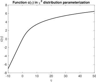
Figure 5: The log-degrees of freedom function $c(\eta)$ related to the $\chi^{2}$-distribution. The plot is obtained using high-precision quadrature and root finding.

A graph of $c(\eta)$ is found in Figure 5. The asymptotic behaviour of $c(\eta)$ is as $0.06756699579940+\eta/\sqrt{2}$ as $\eta\rightarrow-\infty$ and as $2\log(\eta/2)$ as $\eta\rightarrow\infty$. This lead, using similar reasoning as for the $g(a)$ function of the Gamma distribution above, to the approximation $c^{*}(\eta)\approx c(\eta)$ where

$$c^{*}(\eta) =\begin{cases}\frac{1}{2}\log\left(\left\{1+\frac{\eta}{2}\right\}^{4}+\sum_{k=0}^{3}d_{k}\eta^{k}+\sum_{k=4}^{8}\frac{d_{k}}{(\eta+1)^{k-3}}\right),&\eta\geq 0,\\ 0.06756699579940+\eta/\sqrt{2}+\frac{0.06756699579940}{1+\sum_{k=1}^{8}g_{k}\eta^{k}},&\eta<0.\end{cases}$$

Appropriate constants are found to be

$$d_{0} =0.1328187661904628,\;d_{1}=-0.8124042180306501,\;d_{2}=-0.6984149140560064,$$

$$d_{3} =-0.2688718703460384,\;d_{4}=-0.1935917930606054,\;d_{5}=0.7544141784717283e-1,$$

$$d_{6} =-0.1551443919329064e-1,\;d_{7}=0.6217289009833316e-3,\;d_{8}=0.2243193152771084e-3,$$

and

$$g_{1} =-1.043216558395395,\;g_{2}=0.6460991001293077,\;g_{3}=-.2875916175338523,$$

$$g_{4} =0.9904289739460698e-1,\;g_{5}=-0.2754355277497658e-1,\;g_{6}=0.6410214426494266e-2,$$

$$g_{7} =-0.1291969976759803e-2,\;g_{8}=0.2718157192376444e-3.$$

B.1.3 Weibull distribution

The (block-)orthogonal parameterisation (see Table 8) used here was obtained by Cox and Reid (1987), and results in moments

$$E(x) =\lambda\exp(-(\gamma-1)/\alpha)\text{$\Gamma$(}(1+\alpha)/\alpha),$$

$$Var(x) =\lambda^{2}\exp(2(\gamma-1)/\alpha)\left[\Gamma((2+\alpha)/\alpha)-\left\{\Gamma((1+\alpha)/\alpha)\right\}^{2}\right]$$

where $\gamma\approx 0.5772156649$ (Euler’s constant) and $\alpha=\exp(a),\;\lambda=\exp(b)$. This parameterisation is easily mapped to a more conventional parameterisation, e.g. $p(x|k,\lambda^{\prime})\propto x^{k-1}\exp(-(x/\lambda^{\prime})^{k})$ via $k=\alpha$ and $\lambda^{\prime}=c^{-\frac{1}{\alpha}}\lambda$.

B.1.4 $t$-distribution

Based on the formulas for Fisher information found in Lange et al. (1989, Appendix B), an orthogonal parameterisation for the (location-scale) $t$-distribution is found as indicated in Table 8, i.e. such that $E(x|\mu,\lambda,a)=\mu$ and (for degrees of freedom $\exp(a)>2$) $\text{Var}(x|\mu,\lambda,a)=\exp(-\lambda)\exp(3a)/\left(\left\{\exp(a)+1\right\}^{2}\left\{\exp(a)-2\right\}\right)$. However, since the influence of $a$ on the shape diminishes as $a\rightarrow\infty$, a well-behaved constant information parameterisation for $a$ cannot be found, and therefore, the information w.r.t. $a$ is fixed to a constant $r$. Suitable constants, corresponding to the exact Fisher information at $\exp(a)=\{4,10,20\}$ degrees of freedom are $r=\{0.06,0.01,0.003\}$.

B.2 Discrete observations via observed Fisher information

Parameter block		$\mathcal{J}^{\mathcal{C}}$		Comment
Poisson distribution: $p(\mathbf{y}|\theta_{(1)})=\prod_{i=1}^{N}\frac{(\exp(\theta_{(1)})t_{i})^{y_{i}}}{y_{i}!}\exp(-\exp(\theta_{(1)})t_{i})$, $y_{i}\in\{0,1,\dots\}$.
$\theta_{(1)}\in\mathbb{R}$: log-mean		$\sum_{i=1}^{N}y_{i}$		$t_{1},\dots,t_{N}>0$ fixed exposure times.
Binomial distribution: $p(y|\theta)\propto\left(\frac{\exp(\theta_{(1)})}{1+\exp(\theta_{(1)})}\right)^{y}\left(1-\frac{\exp(\theta_{(1)})}{1+\exp(\theta_{(1)})}\right)^{n-y},$ $y\in\{0,1,\dots,n\}$, .
$\theta_{(1)}\in\mathbb{R}$: logit success prob		$\frac{y(n-y)}{n}$		$n$ fixed.
Negative Binomial distribution: $p(y|\theta)=\frac{\Gamma(y+n)}{\Gamma(n)\Gamma(y+1)}\left(\frac{\exp(\theta_{(1)})}{1+\exp(\theta_{(1)})}\right)^{n}\left(1-\frac{\exp(\theta_{(1)})}{1+\exp(\theta_{(1)})}\right)^{y},\;y\in\{0,1,\dots\}.$
$\theta_{(1)}\in\mathbb{R}$: logit success prob		$\frac{ny}{n+y}$		$n>0$ fixed.

Table 9: Parameterisations and information based on observed Fisher information $\mathcal{J}^{\mathcal{C}}$ defined in (19). Note that the information in this case depend on observations $y$.

As discussed above, for observed components in a statistical model, the information with respect to the parameters may be allowed to depend on the observed value without breaking SD properties. This is in particular important for discrete distributions, which per definition are not sampled in the present framework, and also because useful CIPs seems difficult to come by (e.g. for the Poisson distribution, CIPs are on the form $E(y)=c\theta^{2}$, whereas the CIPs for the binomial distribution are on the form $E(y)=\frac{1}{2}+\frac{1}{2}\sin(\theta)$). Thus, Table 9 provides observed Fisher information for some common discrete probability models with canonical link functions.

B.3 GLMs and GLMMs

The observed Fisher information approach can be easily extended to GLM and GLMM settings for observations with linear predictor

$$\eta=\mathbf{X}\beta+\mathbf{F}\delta$$

where $\beta$ are fixed effects and $\delta$ are random effects. In such a situation, joint (expected or observed) Fisher information for $(\beta,\delta)$ can be obtained by fitting the corresponding GLM with $\delta$ treated as a fixed effect using standard software. Alternatively, if this model in not identified, setting the random effects to some central value and calculating the Hessian wrt $\delta$ may also be an option. If the model does not have additional nuisance parameters, this process needs only to be done once.

Appendix C Multivariate Gaussian models

This section considers CIPs for different multivariate Gaussian models, as such models are typically important building blocks for hierarchical Bayesian models. Suppose one is interested in a model on the form

$$\mathbf{x}\sim N(\mathbf{m}(\omega),\mathbf{P}(\lambda)^{-1})$$ (38)

where $\omega$, $\lambda$ are parameter vectors determining the the mean and precision matrix respectively. It is rather straight forward to verify that

1. The Fisher information with respect to $\lambda$ does not depend on $\omega$.

2. The $\lambda,\omega$-cross information is zero.

3. When $\mathbf{m}(\omega)$ is linear in $\omega$, the Fisher information with respect to $\omega$ does not depend on $\omega$ (but generally depends on $\lambda$, specifically linearly in $\mathbf{P}$).

This information suggest that any CIP for a model on the form (38), the first parameter blocks must encode $\lambda$, whereas the last parameter blocks must represent $\omega$. In particular, no information is lost by considering $\lambda$ and $\omega$ in different blocks. In what follows, only linear or constant $\mathbf{m}(\omega)$s are considered as this seems sufficient for the most common applications, whereas focus is primarily on constant information parameterisations of different covariance/precision structures.

C.1 Unrestricted covariance

In order to obtain a block-orthogonal CIP for an unrestricted covariance/precision $n$-dimensional Gaussian distribution that is also convenient in a computational perspective, consider the following specification of the precision matrix $\mathbf{P}$:

$$\mathbf{P}=\mathbf{V}\mathbf{\Lambda}\mathbf{V}^{T}=\tilde{\mathbf{V}}\tilde{\mathbf{V}}^{T},\;\text{where }\tilde{\mathbf{V}}=\mathbf{V}\mathbf{\Lambda}^{\frac{1}{2}}$$ (39)

and

$$\mathbf{\Lambda} =\text{diag}(\exp(\lambda_{1}),\dots,\exp(\lambda_{n})),\;\mathbf{\lambda}\in\mathbb{R}^{n},$$ (40)

$$\mathbf{V} =\left[\begin{array}[]{cccc}1&0&\cdots&0\\ V_{1}^{[1]}&\ddots&\vdots&\vdots\\ \vdots&\cdots&1&0\\ V_{n-1}^{[1]}&\cdots&V_{1}^{[n-1]}&1\end{array}\right],\;\mathbf{V}^{[j]}\in\mathbb{R}^{n-j},\;j=1,\dots,n-1.$$ (45)

This parameterisation, along with the parameter block ordering $\theta_{(1)}=\mathbf{\lambda}$, $\theta_{(2)}=\text{$\mathbf{V}$}^{[n-1]}$, $\mathbf{\theta}_{(3)}=\mathbf{V}^{[n-2]},\dots,\mathbf{\theta}_{(n)}=\mathbf{V}^{[1]}$ is a block-orthogonal CIP with associated diagonal block Fisher informations

$$\mathcal{F}_{\lambda}=\frac{1}{2}\mathbf{I}_{n},$$

$$\mathcal{F}_{\mathbf{V}^{[n-1]}}(\lambda)=\exp(\lambda_{n-1})\mathbf{\Sigma}_{n,n},$$

$$\mathcal{F}_{\mathbf{V}^{[j]}}(\lambda,\mathbf{V}^{[n-1]},\dots,\mathbf{V}^{[j+1]})=\exp(\lambda_{j})\mathbf{\Sigma}_{j+1:n,j+1:n},\;j=n-2,n-3,\dots,1$$

where $\mathbf{\Sigma}=\mathbf{P}^{-1}$ (see proof is in Section C.3).

To operationalise the above construction, notice that the marginal covariance matrices $\Sigma^{(j)}=\mathbf{\Sigma}_{j+1:n,j+1:n},\;j=n-1,\dots,1$ and Fisher informations can be computed recursively by first initialising

$$\text{$\Sigma$}^{(n-1)}=\exp(-\lambda_{n}),\;\mathcal{F}_{\mathbf{V}^{[n-1]}}=\exp(\lambda_{n-1})\Sigma^{(n-1)},$$

and then for each $j=n-2,n-3,\dots,1$:

$$\rho_{j+1} =\Sigma^{(j+1)}\mathbf{V}^{[j+1]},$$

$$\Sigma^{(j)} =\left[\begin{array}[]{cc}\exp(-\lambda_{j+1})+\rho_{j+1}^{T}\mathbf{V}^{[j+1]}&-\rho_{j+1}^{T}\\ -\rho_{j+1}&\Sigma^{(j+1)}\end{array}\right],$$

$$\mathcal{F}_{\mathbf{V}^{[j]}} =\exp(\lambda_{j})\Sigma^{(j)}.$$

This algorithm obtains as follows: Notice first that if $\mathbf{\mathbf{z}}\sim N(0,I_{n})$, then the precision of $\mathbf{\mathbf{x}}=\tilde{\mathbf{V}}^{-T}\mathbf{z}$ will be $\mathbf{P}$. A simple recursion, based on the back-substitution algorithm applied to the triangular solve problem

$$\tilde{\mathbf{V}}^{T}\mathbf{x}=\mathbf{z},$$

can be used to find the required sequence of covariance matrices associated with $\mathbf{x}$. The back substitution algorithm in this cases reduces to:

$$x_{n} =\exp\left(-\frac{\lambda_{n}}{2}\right)z_{n}$$

$$x_{j} =\exp\left(-\frac{\lambda_{j}}{2}\right)z_{j}-\left[\mathbf{V}^{[j]}\right]^{T}\mathbf{x}_{j+1:n},\;j=n-1,n-2,\dots,1.$$

Considering the associated variance, one obtains that $\Sigma_{n,n}=\exp(-\lambda_{n})$. The recursion for the remaining sub-covariance matrices, $j=n-1,n-2,\dots,1$, result in:

$$\mathbf{\mathbf{\rho}}_{j} =\left[\Sigma_{j+1:n,j+1:n}\right]\mathbf{V}^{[j]},$$

$$\Sigma_{j:n,j:n} =\left[\begin{array}[]{cc}\exp(-\lambda_{j})+\left[\mathbf{V}^{[j]}\right]^{T}\mathbf{\rho}_{j}&-\mathbf{\rho}_{j}^{T}\\ -\mathbf{\rho}_{j}&\Sigma_{j+1:n,j+1:n}\end{array}\right].$$

C.1.1 Implied Wishart prior on $P$ in (39)

The Wishart distribution is much used as a prior for unrestricted precision matrices of multivariate Gaussian distributions. Here, a prior density kernel for $\lambda,\mathbf{V}^{[n-1]},\dots,\mathbf{V}^{[1]}$ is given, so that the resulting precision matrix in (39-45) will be Wishart distributed.

Let $0<\mathbf{Q}\in\mathbb{R}^{n\times n}$ and SPD, let and $\mathbf{P}\sim\text{Wishart}_{n}(\mathbf{Q},\nu)$, so that $E(\mathbf{P})=\nu\mathbf{Q}$ and $\nu>n$ is the degrees of freedom parameter. Moreover, let $\mathbf{W}$ be a lower-triangular Cholesky factor of $\mathbf{Q}$. Then, via the Bartlett decomposition,

$$\mathbf{F}(\lambda,\mathbf{V}^{[n-1]},\dots,\mathbf{V}^{[1]})=\mathbf{W}^{-1}\tilde{\mathbf{V}}\sim\mathbf{A},$$

where the lower-triangular matrix $\mathbf{A}$ has independent non-zero elements distributed according to $A_{i,i}\sim\sqrt{\chi_{\nu-i+1}^{2}},\;i=1,\dots,n$ and $A_{i,j}\sim N(0,1),\;j=1,\dots,n-1,\;i=j+1,\dots,n$. The results presented here are based on the standard transformation formula applied to each non-zero element of the transformation $\mathbf{F}(\lambda,\mathbf{V}^{[n-1]},\dots,\mathbf{V}^{[1]})$. The default ordering of the variables leads to a lower tri-diagonal Jacobian with Jacobian determinant proportional to $\exp(\frac{1}{2}\sum_{j=1}^{n}(n-j+1)\lambda_{j})$. This results in the following, independent logarithm of Gamma prior for $\mathbf{\lambda}$,

$$p(\lambda)\propto\exp\left(\sum_{j=1}^{n}\left\{\frac{\nu+n+1}{2}-j\right\}\lambda_{j}-\frac{1}{2}\sum_{j=1}^{n}\frac{\exp(\lambda_{j})}{w_{j,j}^{2}}\right),$$

and corresponding second derivative at optimum- based approximate precision

$$\text{Prec}(\lambda)\approx\text{diag}\left(\left\{\frac{\nu+n+1}{2}-j\right\}_{j=1}^{n}\right),$$

required for the $\mathcal{I}^{\mathcal{A}}$ associated with $\lambda$. Next, the conditional (on $\lambda$) prior for $\mathbf{V}^{[j]},$ $j=n-1,n-2,\dots,1,$ is given as

$$p(\mathbf{V}^{[j]}|\mathbf{\lambda})\propto\exp\left(-\frac{1}{2}\sum_{k=j+1}^{n}\mathbf{F}_{k,j}^{2}\right),$$

which, via straight forward manipulations is Gaussian with precision

$$\text{Prec($\mathbf{V}$}^{[j]}|\lambda)=\exp(\lambda_{j})\left[\mathbf{Q}^{-1}\right]_{j+1:n,j+1:n}.$$

Note that conditionally on $\mathbf{\lambda}$, the priors for the columns of $\mathbf{V}$ are independent, and also that $\mathbf{W}$ and $\mathbf{Q}^{-1}$ may be pre-computed.

C.2 Restricted Multivariate Gaussian models

parameter		Information		Comment
blocks
Independent, identical variance: $\mathbf{x}\sim N(\mathbf{v}+\mathbf{X}\beta,\exp(-\lambda)\mathbf{I}_{n})$,
$\mathbf{v}\in\mathbb{R}^{n},\;\mathbf{X}\in\mathbb{R}^{n\times p}$ are not sampled.
$\theta_{(1)}=\lambda\in\mathbb{R}$: log-precision		$\frac{n}{2}$
$\theta_{(2)}=\mathbf{\beta}\in\mathbb{R}^{p}$: regression coeff.		$\exp(\lambda)\mathbf{X}^{T}\mathbf{X}$
Independent, different variances: $\mathbf{x}\sim N(\mathbf{v}+\mathbf{X}\beta,\text{diag}(\exp(-\lambda_{1}),\dots,\exp(-\lambda_{n}))),$
$\mathbf{v}\in\mathbb{R}^{n},\;\mathbf{X}\in\mathbb{R}^{n\times p}$ are not sampled.
$\theta_{(1)}=\lambda\in\mathbb{R}^{n}$: log-precisions		$\frac{1}{2}\mathbf{I}_{n}$
$\theta_{(2)}=\beta\in\mathbb{R}^{p}$: regression coeff.		$\mathbf{X}^{T}\text{diag}(\exp(\lambda_{1}),\dots,\exp(\lambda_{n}))\mathbf{X}$
Unrestricted precision: $\mathbf{x}\sim N(\mathbf{v}+\mathbf{X}\beta,\mathbf{P}^{-1})$, where $\mathbf{v}\in\mathbb{R}^{d}$, $\mathbf{X}\in\mathbb{R}^{d\times p}$ are not sampled.
See Section C.1 for definition of $\mathbf{P}=\mathbf{P}(\lambda,\mathbf{V})$.
$\theta_{(1)}=\lambda\in\mathbb{R}^{d}$		$\frac{1}{2}\mathbf{I}_{d}$
$\theta_{(2)}=\mathbf{V}^{[d-1]}\in\mathbb{R}$		$\exp(\lambda_{d-1})(\mathbf{P}^{-1})_{d,d}$
$\vdots$		$\vdots$
$\theta_{(d)}=\mathbf{V}^{[1]}\in\mathbb{R}^{d-1}$		$\exp(\lambda_{1})(\mathbf{P}^{-1})_{2:d,2:d}$
$\theta_{(d+1)}=\beta\in\mathbb{R}^{p}$: regression coeff.		$\mathbf{X}^{T}\mathbf{P}\mathbf{X}$
Stationary Gaussian AR(1) model: $x_{t+1}|x_{t}\sim N(\mu+\phi(\omega)(x_{t}-\mu),\exp(-\lambda))$,
$x_{1}\sim N\left(\mu,\frac{\exp(-\lambda)}{1-\phi(\omega)^{2}}\right)$,
$\theta_{(1)}=\lambda\in\mathbb{R}$: noise log-precision		$\frac{T}{2}$		See section C.2.1.
$\theta_{(2)}=\omega\in\mathbb{R}$: mapped autocorrelation		$\frac{T}{2}$
$\theta_{(3)}=\mu\in\mathbb{R}$: marginal mean		$\exp(\lambda)\left[2(T-1)(1-\phi(\omega))-\frac{T-2}{\cosh(\psi(\omega))^{2}}\right]$
Intrinsic RW(1) model: $p(x|\lambda)\propto\exp(\lambda)^{(T-1)/2}\exp(-\frac{1}{2}\exp(\lambda)\sum_{t=2}^{T}(x_{i}-x_{i-1})^{2}),\;\mathbf{x}\in\mathbb{R}^{T},\;T\geq 2$.
$\theta_{(1)}=\lambda\in\mathbb{R}$: noise log-precision		$\frac{T-1}{2}$
Intrinsic RW(2) model: $p(x|\lambda)\propto\exp(\lambda)^{(T-2)/2}\exp(-\frac{1}{2}\exp(\lambda)\sum_{t=3}^{T}(x_{t}-2x_{t-1}+x_{t-2})^{2}),$
$\mathbf{x}\in\mathbb{R}^{T},\;T\geq 3$.
$\theta_{(1)}=\lambda\in\mathbb{R}$: noise log-precision		$\frac{T-2}{2}$
Besag-type Intrinsic GMRF: $\mathbf{x}\in\mathbb{R}^{n}$, $x_{i}|\mathbf{x}_{-i},\text{$\lambda$}\sim N(\frac{1}{n_{i}}\sum_{i\sim j}x_{j},(n_{i}\exp(\lambda))^{-1})$ where $i\sim j$ indicate that
nodes $i,j$ are neighbours, and $n_{i}$ is the number of neighbours.
$\theta_{(1)}=\lambda\in\mathbb{R}:$ log-precision		$\frac{n-1}{2}$

Table 10: CIPs for structured multivariate (intrinsic) Gaussian models. The CIPs are block orthogonal except for the stationary Gaussian AR(1) model which is asymptotically (in $T$) block orthogonal. The results for the intrinsic models obtains via limit arguments.

An overview of block-orthogonal CIPs for several multivariate Gaussian models are presented in Table 10. Again, most of the results presented are straight forward obtain, and therefore only the stationary Gaussian AR(1) model is discussed in detail:

C.2.1 Stationary Gaussian AR(1)

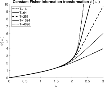
Figure 6: The function $\psi(\omega)$ associated with autoregressive parameters in a stationary Gaussian AR(1) process. Only the positive arguments are considered as $\psi(\omega)=-\psi(-\omega)$.

Figure 7: The $(\lambda,\omega)$-correlation associated with $\mathcal{F}_{(\lambda,\omega)}$ interpreted as precision matrix. The curves as anti-symmetric $(\rho(\omega)=-\rho(-\omega)$) and therefore only non-negative values of $\omega$ are considered.

Re-consider the stationary AR(1) model (22,23) with parameters $(\lambda,\omega,\mu)$ which will have an asymptotically block orthogonal CIP property. For simplicity, it is assumed that $T>3$. Tedious, but trivial calculations lead to the Fisher information associated with $(\lambda,\omega,\mu)$ being

$$\mathcal{F}_{(\lambda,\omega,\mu)}=\left[\begin{array}[]{ccc}\frac{T}{2}&\text{sym}&\text{\text{sym}}\\ -\left(\frac{d}{d\omega}\psi(\omega)\right)\tanh(\psi(\omega))&\left(\frac{d}{d\omega}\psi(\omega)\right)^{2}\left[2+\frac{T-3}{\cosh(\psi(\omega))^{2}}\right]&\text{sym}\\ 0&0&\exp(\lambda)\left[2(T-1)(1-\phi(\omega))-\frac{T-2}{\cosh(\psi(\omega))^{2}}\right]\end{array}\right].$$

In what follows, $\psi(\omega)$ is chosen so that $\mathcal{F}_{\omega,\omega}=\left(\frac{d}{d\omega}\psi(\omega)\right)^{2}\left[2+\frac{T-3}{\cosh(\psi(\omega))^{2}}\right]=\frac{T}{2}$, $\psi(0)=0$ and $\frac{d}{d\omega}\psi(\omega)>0$ (the differential equation admit both monotonously increasing and decreasing solutions). Under these constraints, $\psi(\omega)$ solves

$$\omega=\int_{0}^{\psi(\omega)}u(a)da,\;u(a)=\frac{2}{\sqrt{T}}\frac{\sqrt{(\exp(a)+\exp(-a))^{2}+2(T-3)}}{\exp(a)+\exp(-a)}$$ (46)

where the right hand side integral has a closed (but complicated) form which can be used in numerical computation of $\psi$. Note that $u(a)=u(-a)\;\forall a$, which implies that $\psi(\omega)=-\psi(-\omega)\;\forall\omega$. The shape of $\psi$ for different values of $T$ is illustrated in Figure 6. Note in particular that $\lim_{|\omega|\rightarrow\infty}\frac{\psi(\omega)}{\frac{\sqrt{T}}{2}\omega}=1$, which is relatively easy too see from (46) since the integrand tends to $2/\sqrt{T}$ as $|a|\rightarrow\infty$.

To argue that the $\mathcal{F}_{\lambda,\omega}$ information is asymptotically irrelevant, it is clear that

$$|\mathcal{F}_{\lambda,\omega}|=|\tanh(\psi(\omega))|\frac{1}{u(\psi(\omega))}\leq\frac{1}{u(\psi(\omega))}\leq\frac{\sqrt{T}}{2},$$

where the latter inequality stems from the fact that $u(a)$ is minimised as $|a|\rightarrow\infty$, for which we have that $\lim_{|a|\rightarrow\infty}u(a)=\frac{2}{\sqrt{T}}$. Based on these calculations, it is clear that an upper bound on the correlation associated with $\mathcal{F}_{(\lambda,\omega)}$ (i.e. with $\mathcal{F}_{(\lambda,\omega)}^{-1}$ interpreted as a covariance matrix) is $|\rho|\leq T^{-\frac{1}{2}}$. In practice, these correlations are negligible as shown in Figure 7. In what follows, it will therefore with little or no loss of efficiency, be sufficient to consider the CIP blocking $\theta_{(1)}=\lambda$, $\theta_{(2)}=\omega$ and $\theta_{(3)}=\mu$ (the ordering of $\lambda$ and $\omega$ is arbitrary).

C.3 Proof of block orthogonal CIP for unrestricted Gaussian variance

A multivariate Gaussian distribution for random vector $\mathbf{x}$ with mean $\mathbf{\mu}$ and covariance matrix $\mathbf{\Sigma}=\mathbf{P}^{-1}$ is considered, i.e. $p(\mathbf{x}|\mathbf{\mu},\mathbf{P})=\mathcal{N}(\mathbf{x}|\mathbf{\mu},\mathbf{P}^{-1})$ where the parameterisation of $\mathbf{P}$ is given in (39-45).

C.3.1 $\lambda$ information

Straight forward calculations lead to

$$\nabla_{\mathbf{\lambda}}\log p(\mathbf{x}|\mathbf{\mathbf{\mu}},\mathbf{P})=-\frac{1}{2}\text{diag}\left(\tilde{\mathbf{V}}^{T}(\mathbf{x}-\mathbf{\mathbf{\mu}})\right)\tilde{\mathbf{V}}^{T}(\mathbf{x}-\mathbf{\mu})+\frac{1}{2}\mathbf{1}_{n},$$

where $\mathbf{1}_{n}=[1,\dots,1]^{T}\in\mathbb{R}^{n}$. Taking outer product, and substituting $\mathbf{x}=\mathbf{\mu}+\tilde{\mathbf{V}}^{-T}\mathbf{z}$, $\mathbf{z}\sim N(0,\mathbf{I}_{n})$ (in order to simplify the subsequent expectation calculations), so that $S(\mathbf{z})=\left[\nabla_{\lambda}\log p(\mathbf{x}|\mathbf{\mu},\mathbf{P})\right]\left[\nabla_{\lambda}\log p(\mathbf{x}|\mathbf{\mu},\mathbf{P})\right]^{T}|_{\mathbf{x}=\mathbf{\mu}+\tilde{\mathbf{V}}^{-T}\mathbf{z}}$ one obtains that

$$\mathbf{S}(\mathbf{z})=\frac{1}{4}\text{diag}(\mathbf{z})\mathbf{z}\mathbf{z}^{T}\text{diag}(\mathbf{z})-\frac{1}{4}\text{diag}(\mathbf{z})\mathbf{z}\mathbf{1}_{n}^{T}-\frac{1}{4}\mathbf{1}_{n}\mathbf{z}^{T}\text{diag}(\mathbf{z})+\frac{1}{4}\mathbf{1}_{n}\mathbf{1}_{n}^{T}.$$

Thus

$$S_{i,j}(\mathbf{z})=\frac{1}{4}\left(z_{i}^{2}z_{j}^{2}-z_{i}^{2}-z_{j}^{2}+1\right),$$

and finally

$$\mathcal{F}_{1} =\underset{\mathbf{z}}{E}\left[\mathbf{S}(\mathbf{z})\right]=\frac{1}{2}I_{n}.$$

C.3.2 $V^{[j]},\;j=1,\dots,n-1$ information

Notice first (as $|\mathbf{V}|=1$) that

$$\log p(\mathbf{x}|\mathbf{\mu},\mathbf{P})=-\frac{1}{2}\left(\tilde{\mathbf{V}}^{T}\left(\mathbf{x}-\mathbf{\mu}\right)\right)^{T}\tilde{\mathbf{V}}^{T}\left(\mathbf{x}-\mathbf{\mu}\right)+\text{constant},$$

when $\lambda$ is fixed. Straight forward calculations lead to that

$$\nabla_{\mathbf{V}^{[j]}}\tilde{\mathbf{V}}^{T}\left(\mathbf{x}-\mathbf{\mu}\right)=\exp\left(\frac{\lambda_{j}}{2}\right)\mathbf{e}_{j}\left[\left(\mathbf{x}-\mathbf{\mu}\right)_{j+1:n}\right]^{T}\in\mathbb{R}^{n\times n-j},$$ (47)

where $\mathbf{e}_{j}\in\mathbb{R}^{n}$ is the $j$th unit vector. Thus

$$\nabla_{\mathbf{V}^{[j]}}\log p(\mathbf{x}|\mathbf{\mu},\mathbf{P})=-\exp\left(\frac{\lambda_{j}}{2}\right)\left(\mathbf{x}-\mathbf{\mu}\right)_{j+1:n}\mathbf{e}_{j}^{T}\tilde{\mathbf{V}}^{T}\left(\mathbf{x}-\mathbf{\mu}\right),$$ (48)

and

$$-\nabla_{\mathbf{V}^{[j]}}^{2}\log p(\mathbf{x}|\mathbf{\mu},\mathbf{P})=\exp(\lambda_{j})\left(\mathbf{x}-\mathbf{\mu}\right)_{j+1:n}\underbrace{\mathbf{e}_{j}^{T}\mathbf{e}_{j}}_{=1}\left[\left(\mathbf{x}-\mathbf{\mu}\right)_{j+1:n}\right]^{T}.$$

Thus

$$\mathcal{F}_{\mathbf{V}^{[k]}}=E\left[-\nabla_{\mathbf{V}^{[j]}}^{2}\log p(\mathbf{x}|\mathbf{\mu},\mathbf{P})\right]=\exp(\lambda_{j})\Sigma_{j+1:n,j+1:n}.$$

This shows the general $\mathcal{F}_{\mathbf{V}^{[j]}}$-formula.

To show that $\mathcal{F}_{\mathbf{V}^{[j]}}$ depends only on $\lambda,\mathbf{V}^{[j+1]},\dots,\mathbf{V}^{[n-1]}$, observe that $\mathbf{x}$ can be simulated as $\mathbf{x}=\mathbf{\mu}+\tilde{\mathbf{V}}^{-T}\mathbf{z}$ or, explicitly by back-substitution based on $\tilde{\mathbf{V}}^{T}(\mathbf{x}-\mathbf{\mu})=\mathbf{z}$. I.e. $x_{n}$ (whose variance is needed calculation of $\mathcal{F}_{\mathbf{V}^{[n-1]}}$) obtains from

$$\exp(\lambda_{n}/2)(x_{n}-\mathbf{\mu}_{n})=z_{n}$$

i.e. depends only on $\lambda_{n}$. Continuing the recursion, we have that $x_{n-1}$ (variance of $x_{n-1:n}$ needed in calculation of $\mathcal{F}_{\mathbf{V}^{[n-2]}}$) of obtains from

$$\exp(\lambda_{n-1}/2)\left((x_{n-1}-\mu_{n-1})+\mathbf{V}_{1}^{[n-1]}(x_{n}-\mu_{n})\right)=z_{n-1},$$

i.e. depends only on $\lambda_{n-1:n}$ and $\mathbf{V}^{[n-1]}$. To get the remaining dependencies, the recursion is simply continued.

C.3.3 The cross-informations are zero:

Consider first the $(\mathbf{V}_{[j]}$ , $\mathbf{V}_{[k]})$, $k\neq j$ cross information. Take as vantage point (48) and (47) to obtain that

$$\nabla_{\mathbf{V}^{[j]},\mathbf{V}^{[k]}}^{2}\log p(\mathbf{x}|\mathbf{\mu},\mathbf{P}) =\nabla_{\mathbf{V}^{[k]}}\left[\nabla_{\mathbf{V}^{[j]}}\log p(\mathbf{x}|\mathbf{\mu},\mathbf{P})\right]\in\mathbb{R}^{n-j\times n-k}$$

$$=\left[-\exp\left(\frac{\lambda_{j}}{2}\right)\left(\mathbf{x}-\mathbf{\mu}\right)_{j+1:n}\mathbf{e}_{j}^{T}\right]\left[\nabla_{\mathbf{V}^{[k]}}\tilde{\mathbf{V}}^{T}\left(\mathbf{x}-\mathbf{\mu}\right)\right]$$

$$=-\exp\left(\frac{\lambda_{j}+\lambda_{k}}{2}\right)\left(\mathbf{x}-\mathbf{\mu}\right)_{j+1:n}\underbrace{\mathbf{e}_{j}^{T}\mathbf{e}_{k}}_{=0}\left[\left(\mathbf{x}-\mathbf{\mu}\right)_{k+1:n}\right]^{T}$$

$$=\mathbf{0}_{n-j\times n-k}$$

i.e. the $(n-j)$ times $(n-k)$-zero matrix.

Now for the $(\lambda$ , $\mathbf{V}_{[j]})$ cross information, again take as vantage point (48) to obtain

$$\nabla_{\lambda,\mathbf{V}^{[j]}}^{2}\log p(\mathbf{x}|\mathbf{\mu},\mathbf{P}) =\nabla_{\lambda}\left[\nabla_{\mathbf{V}^{[j]}}\log p(\mathbf{x}|\mathbf{\mu},\mathbf{P})\right]\in\mathbb{R}^{n-j\times n}$$

$$=\nabla_{\lambda}\left[-\exp\left(\frac{\lambda_{j}}{2}\right)\left(\mathbf{x}-\mathbf{\mu}\right)_{j+1:n}\mathbf{e}_{j}^{T}\tilde{\mathbf{V}}^{T}\left(\mathbf{x}-\mathbf{\mu}\right)\right]$$

$$=\nabla_{\lambda}\left[-\exp\left(\frac{\lambda_{j}}{2}\right)\left(\mathbf{x}-\mathbf{\mu}\right)_{j+1:n}(\mathbf{e}_{j}^{T}\Lambda)L^{T}\left(\mathbf{x}-\mathbf{\mu}\right)\right]$$

$$=\nabla_{\lambda}\left[-\exp\left(\lambda_{j}\right)\left(\mathbf{x}-\mathbf{\mu}\right)_{j+1:n}\mathbf{e}_{j}^{T}L^{T}\left(\mathbf{x}-\mathbf{\mu}\right)\right]$$

It is seen that $\nabla_{\mathbf{V}^{[j]}}\log p(\mathbf{x}|\mathbf{\mu},\mathbf{P})$ only depends on $\lambda_{j}$, and thus

$$\frac{\partial}{\partial\lambda_{k}}\left[\nabla_{\mathbf{V}^{[j]}}\log p(\mathbf{x}|\mathbf{\mu},\mathbf{P})\right]=0,\;\text{for}\;j\neq k.$$

Further, it remains to look at

$$E\left[\frac{\partial}{\partial\lambda_{j}}\left[\nabla_{\mathbf{V}^{[j]}}\log p(\mathbf{x}|\mathbf{\mu},\mathbf{P})\right]\right] =E\left[-\exp\left(\lambda_{j}\right)\left(\mathbf{x}-\mathbf{\mu}\right)_{j+1:n}\mathbf{e}_{j}^{T}L^{T}\left(\mathbf{x}-\mathbf{\mu}\right)\right]$$

$$=E\left[-\exp\left(\frac{\lambda_{j}}{2}\right)\left(\mathbf{x}-\mathbf{\mu}\right)_{j+1:n}\mathbf{e}_{j}^{T}\tilde{\mathbf{V}}^{T}\left(\mathbf{x}-\mathbf{\mu}\right)\right]$$

Now, we substitute $\mathbf{x}=\mathbf{\mu}+\tilde{\mathbf{V}}^{-T}\mathbf{z}$, $\mathbf{z}\sim N(0,\mathbf{I}_{n})$ to obtain

$$E\left[\frac{\partial}{\partial\lambda_{j}}\left[\nabla_{\mathbf{V}^{[j]}}\log p(\mathbf{x}|\mathbf{\mu},\mathbf{P})\right]\right]=-\exp\left(\frac{\lambda_{j}}{2}\right)E\left[\left(\tilde{\mathbf{V}}^{-T}\mathbf{z}\right)_{j+1:n}z_{j}\right].$$

Now, $(\tilde{\mathbf{V}}^{-T}\mathbf{z})_{j+1:n}$ depends only on $\mathbf{z}_{j+1:n}$ (see last part of section C.3.2) and therefore

$$-\exp\left(\frac{\lambda_{j}}{2}\right)E\left[E_{z_{j}}\left[\left(\tilde{\mathbf{V}}^{-T}\mathbf{z}\right)_{j+1:n}z_{j}|\mathbf{z}_{j+1:n}\right]\right]=\mathbf{0}_{n-j,1}.$$

This completes the proof that the parameterisation of $\mathbf{P}$ is given in (39-45) with parameter blocks $\theta_{(1)}=\lambda$, $\theta_{(2)}=\mathbf{V}^{[n-1]},\dots,$ $\theta_{(n)}=\mathbf{V}^{[1]}$ is a block-orthogonal CIP.

Appendix D Stan implementation and CIPlib

This section gives some directions on how to implement DRHMC with Stan. Moreover, some details of the Stan functions in the R-package CIPlib used in the illustrations of the paper are given. CIPlib can be downloaded from http://www.ux.uis.no/~tore/DRHMC/CIPlib/ or alternatively, be installed directly (for Unix-like systems) via the R command 
install.packages("http://www.ux.uis.no/~tore/DRHMC/CIPlib/CIPlib_1.0.tar.gz").

D.1 Implementing DRHMC in Stan

This section assumes some experience in writing models in the Stan language. Before providing step-by-step directions, it is convenient to introduce Stan codes for the simple illustration model (14,16). An implementation in the original $(\mathbf{q}_{(1)},\mathbf{q}_{(2)})$ parameterisation obtains as
 

⬇

1data{

2 real y;

3}

4parameters{

5 real q1;

6 real q2;

7}

8model{

9 // "priors"

10 target += normal_lpdf(q1 | 0.0 , 1.0);

11 target += normal_lpdf(q2 | 0.0 , 1.0);

12 // "likelihood"

13 target += normal_lpdf(y | q2 , exp(-1.5*q1)); // notice: standard deviation

14}

 

In the DRHMC parameterisation $(\bar{\mathbf{q}}_{(1)},\bar{\mathbf{q}}_{(2)})$, the relevant Stan code is
 

⬇

1data{

2 real y;

3}

4parameters{

5 real q1_bar;

6 real q2_bar;

7}

8transformed parameters{

9 real q1;

10 real q2;

11 real h2;

12 real L2;

13 // first block variable transformation: G_(1)=1+9/2

14 q1 = q1_bar/sqrt(1.0+4.5);

15

16 // now q1 is available, can compute h_(2) and L_(2)

17 h2 = y/(1.0+exp(-3.0*q1)); // = E(q2|q1,y)

18 L2 = sqrt(1.0+exp(3.0*q1));

19

20 // second block variable transformation:

21 q2 = h2 + q2_bar/L2;

22}

23model{

24 // "priors"

25 target += normal_lpdf(q1 | 0.0 , 1.0);

26 target += normal_lpdf(q2 | 0.0 , 1.0);

27 // "likelihood"

28 target += normal_lpdf(y | q2 , exp(-1.5*q1)); // notice: standard deviation

29 // contribution from Jacobian

30 target += -log(L2);

31}

 

The steps taken to prepare a Stan code implementing (11) for DRHMC are:

1. Change the names of the “sampled” parameters in the parameters block to the names of the corresponding standardised variables (lines 5,6 in DRHMC code)

2. Augment (or introduce) the transformed parameters block with the evaluation of $\mathbf{q}=\Psi(\bar{\mathbf{q}})$ (lines 8-22 in DRHMC code). This is done sequentially by iterating between evaluating $\mathbf{L}_{(r)},\mathbf{h}_{(r)}$ and computing $\mathbf{q}_{(r)}$. It is good practice to let the names of the variables resulting from this process be the original names (i.e. here q1,q2).

3. The model block remains the same except that the value of the target log-density must be incremented with logarithm of the Jacobian determinant, $-\sum_{r=2}^{R}\log(|\mathbf{L}_{(r)}|)$ (line 30 in DRHMC code).

As demonstrated, this process is conceptually straightforward. However, for more complicated models, the implementation of $\mathbf{q}=\Psi(\bar{\mathbf{q}})$ may involve e.g. specialised linear algebra functions or functions related to CIPs.

D.2 The R package CIPlib

The R-package CIPlib provides utilities for doing DRHMC within RStan. The Stan code “headers” are easily extracted from the package and can thus be used with Stan under other environments. The instructions for using CIPlib (after installation and loading) with RStan are as follows:

1. Put < #include "CIPlib.stan" > inside the functions{} block at the start of your Stan model file.

2. Translate the Stan model using stanc_builder() with arguments
   < allow_undefined=TRUE, isystem=CIP_header_path() >.

3. Compile the Stan model using stan_model() with arguments
   < allow_undefined=TRUE, include=CIP_include() >.

4. Run the model using sampling().

The implementations in CIPlib relevant for the illustrations in the present paper are:

• The function $\psi(\omega)$ involved in the CIP for the stationary Gaussian AR(1) process is available psi = CIP_AR1_psi(omega,T) where $T$ is the sample size. The evaluation and calculation of derivatives relies on C++ code, and an R-interface is also available.

• The function $\xi(T)$, the second order derivative-based approximation to the implied prior on $\omega$ when $\frac{1}{2}\left(\phi(\omega)+1\right)\sim\text{Beta}(\alpha,\beta),$ is available as xi = CIP_AR1_omega_defaultPrior_prec(alpha,beta,T).

• Cholesky factorisation for tri-diagonal $T\times T$ matrices on the form

  $$\mathbf{G}=\left[\begin{array}[]{ccccc}a&c\\ c&b&c\\ &\ddots&\ddots&\ddots\\ &&c&b&c\\ &&&c&a\end{array}\right]$$

  is provided in L=CIP_TriDiagChol_const1n(T,a,b,c) where L is a $2T$ vector with L[1:2*T-1] containing a representation of the lower Cholesky factor, and L[2*T] is the log-determinant of L.

• Cholesky factorisation for tri-diagonal $T\times T$ matrices on the form

  $$\mathbf{G}=\left[\begin{array}[]{ccccc}v_{1}&c_{1}\\ c_{1}&v_{2}&c_{2}\\ &\ddots&\ddots&\ddots\\ &&c_{T-2}&v_{T-1}&c_{T-1}\\ &&&c_{T-1}&v_{T}\end{array}\right]$$

  is provided in L=CIP_TriDiagChol(v,c). The output is as above.

• The routines for solving $L^{T}x=y$, $Lx=y$ and $LL^{T}x=y$ when L is output from either tridiagonal Cholesky algorithm above, are x=CIP_TriDiagChol_LT_solve(L,y), x=CIP_TriDiagChol_L_solve(L,y) and x=CIP_TriDiagChol_LLT_solve(L,y) respectively.

Appendix E Details on RMHMC and SSHMC references

This section discusses implementation details for the reference methods considered in the linear Gaussian state space model example in section 5.1.

E.1 RMHMC

The RMHMC method used is that of Kleppe (2018). In particular, this method exploits that $p(\mathbf{x}|\mathbf{y},\lambda,\tau)$ is log-concave. Throughout, a step size of 0.1 was applied, and the number of integration steps were uniformly distributed between 30 and 50. The remaining regularisation parameters $u_{101}$, (and $u_{102}$ for model 3) were all set equal to $\exp(4)$.

E.2 Semi-separable Hamiltonian Monte Carlo

The semi-separable Hamiltonian Monte Carlo (SSHMC) (Zhang and Sutton, 2014) using the alternating block-wise leapfrog algorithm (ABLA) was implemented with the block-diagonal metric tensor identical to those used for DRHMC. Similar choices were done by Zhang and Sutton (2014, section 5.3) for a stochastic volatility model. Here, only model 3 is considered, whereas straight forward modifications lead to the remaining models 1 and 2. Let $\phi=(\lambda,\tau)^{T}$ and let the Hamiltonian in question is given by

$$\text{$\mathcal{H}$}_{\text{SSHMC}}(\phi,\mathbf{x},\mathbf{p}_{\phi},\mathbf{p}_{\mathbf{x}})= -\log p(\mathbf{y}|\mathbf{x},\text{$\tau$})-\log p(\mathbf{x}|\lambda)-\log p(\tau)$$

$$+\frac{1}{2}\mathbf{p}_{\phi}^{T}\mathbf{G}_{(1)}^{-1}\mathbf{p}_{\phi}+\frac{1}{2}\log(|\mathbf{G}_{(2)}(\phi)|)+\frac{1}{2}\mathbf{p}_{\mathbf{x}}^{T}\mathbf{G}_{(2)}^{-1}(\phi)\mathbf{p}_{\mathbf{x}}.$$

SSHMC relies on considering the time dynamics in either $(\phi,\mathbf{p}_{\phi})$ or $(\mathbf{x},\mathbf{p}_{\mathbf{x}})$ (while keeping the opposite constant) separately. Up to additive constants, this results in two separable Hamiltonians

$$\mathcal{H}_{\text{SSHMC},\phi}(\phi,\mathbf{p}_{\phi}) =-\log p(\mathbf{y}|\mathbf{x},\text{$\tau$})-\log p(\mathbf{x}|\lambda)-\log p(\tau)+\frac{1}{2}\log(|\mathbf{G}_{(2)}(\phi)|)+\frac{1}{2}\mathbf{p}_{\mathbf{x}}^{T}\mathbf{G}_{(2)}^{-1}(\phi)\mathbf{p}_{\mathbf{x}}+\frac{1}{2}\mathbf{p}_{\phi}^{T}\mathbf{G}_{(1)}^{-1}\mathbf{p}_{\phi},$$

$$\mathcal{H}_{\text{SSHMC},\mathbf{x}}(\mathbf{x},\mathbf{p}_{\mathbf{x}}) =-\log p(\mathbf{y}|\mathbf{x},\text{$\tau$})-\log p(\mathbf{x}|\lambda)+\frac{1}{2}\mathbf{p}_{\mathbf{x}}^{T}\mathbf{G}_{(2)}^{-1}(\phi)\mathbf{p}_{\mathbf{x}},$$

which may be time-integrated numerically using the leap frog method. In each case of the simulation study, 10 ABLA integration steps, each consisting of

• 6 leapfrog steps applied to $\mathcal{H}_{\text{SSHMC},\phi}(\phi,\mathbf{p}_{\phi})$ with step size 0.7,

• 1 leapfrog step applied to $\mathcal{H}_{\text{SSHMC},\mathbf{x}}(\mathbf{x},\mathbf{p}_{\mathbf{x}})$ with step size 0.25,

• 6 leapfrog steps applied to $\mathcal{H}_{\text{SSHMC},\phi}(\phi,\mathbf{p}_{\phi})$ with step size 0.7,

where applied to generate each proposal.

References

- Andrieu et al. (2010) Andrieu, C., A. Doucet, and R. Holenstein (2010). Particle Markov chain Monte Carlo methods. Journal of the Royal Statistical Society: Series B (Statistical Methodology) 72(3), 269–342.
- Betancourt (2013) Betancourt, M. (2013). A general metric for Riemannian manifold Hamiltonian Monte Carlo. In F. Nielsen and F. Barbaresco (Eds.), Geometric Science of Information, Volume 8085 of Lecture Notes in Computer Science, pp. 327–334. Springer Berlin Heidelberg.
- Betancourt (2017) Betancourt, M. (2017). A conceptual introduction to Hamiltonian Monte Carlo. arXiv:1701.02434.
- Carpenter et al. (2017) Carpenter, B., A. Gelman, M. Hoffman, D. Lee, B. Goodrich, M. Betancourt, M. Brubaker, J. Guo, P. Li, and A. Riddell (2017). Stan: A probabilistic programming language. Journal of Statistical Software 76(1), 1–32.
- Cox and Reid (1987) Cox, D. R. and N. Reid (1987). Parameter orthogonality and approximate conditional inference. Journal of the Royal Statistical Society. Series B (Methodological) 49(1), 1–39.
- Davis (2006) Davis, T. A. (2006). Direct Methods for Sparse Linear Systems, Volume 2 of Fundamentals of Algorithms. SIAM.
- Duane et al. (1987) Duane, S., A. Kennedy, B. J. Pendleton, and D. Roweth (1987). Hybrid Monte Carlo. Physics Letters B 195(2), 216 – 222.
- Durbin and Koopman (2012) Durbin, J. and S. J. Koopman (2012). Time Series Analysis by State Space Methods (2 ed.). Number 38 in Oxford Statistical Science. Oxford University Press.
- Fernandez-Villaverde and Rubio-Ramirez (2007) Fernandez-Villaverde, J. and J. F. Rubio-Ramirez (2007). Estimating macroeconomic models: A likelihood approach. Review of Economic Studies 74(4), 1059–1087.
- Flury and Shephard (2011) Flury, T. and N. Shephard (2011). Bayesian inference based only on simulated likelihood: Particle filter analysis of dynamic economic models. Econometric Theory 27(Special Issue 05), 933–956.
- Gelman et al. (2014) Gelman, A., J. B. Carlin, H. S. Stern, D. B. Dunson, A. Vehtari, and D. Rubin (2014). Bayesian Data Analysis (3 ed.). CRC Press.
- Girolami and Calderhead (2011) Girolami, M. and B. Calderhead (2011). Riemann manifold Langevin and Hamiltonian Monte Carlo methods. Journal of the Royal Statistical Society: Series B (Statistical Methodology) 73(2), 123–214.
- Goldstein et al. (2002) Goldstein, H., C. Poole, and J. Safko (2002). Classical Mechanics (3 ed.). Addison Wesley.
- Griewank (2000) Griewank, A. (2000). Evaluating Derivatives: Principles and Techniques of Algorithmic Differentiation. SIAM, Philadelphia.
- Grothe et al. (2016) Grothe, O., T. S. Kleppe, and R. Liesenfeld (2016). The Gibbs sampler with particle efficient importance sampling for state-space models. Econometric Reviews. Forthcoming.
- Hoffman and Gelman (2014) Hoffman, M. D. and A. Gelman (2014). The no-u-turn sampler: Adaptively setting path lengths in Hamiltonian Monte Carlo. Journal of Machine Learning Research 15, 1593–1623.
- Jacquier et al. (1994) Jacquier, E., N. G. Polson, and P. E. Rossi (1994). Bayesian analysis of stochastic volatility models. Journal of Business & Economic Statistics 12(4), 371–89.
- Kim et al. (1998) Kim, S., N. Shephard, and S. Chib (1998). Stochastic volatility: Likelihood inference and comparison with ARCH models. Review of Economic Studies 65(3), 361–93.
- Kleppe (2018) Kleppe, T. S. (2018). Modified cholesky riemann manifold hamiltonian monte carlo: exploiting sparsity for fast sampling of high-dimensional targets. Statistics and Computing 28(4), 795–817.
- Kleppe and Skaug (2012) Kleppe, T. S. and H. J. Skaug (2012). Fitting general stochastic volatility models using Laplace accelerated sequential importance sampling. Computational Statistics & Data Analysis 56(11), 3105 – 3119.
- Kristensen et al. (2016) Kristensen, K., A. Nielsen, C. Berg, H. Skaug, and B. Bell (2016). TMB: Automatic differentiation and Laplace approximation. Journal of Statistical Software 70(1), 1–21.
- Lan et al. (2015) Lan, S., V. Stathopoulos, B. Shahbaba, and M. Girolami (2015). Markov chain Monte Carlo from Lagrangian dynamics. Journal of Computational and Graphical Statistics 24(2), 357–378.
- Lange et al. (1989) Lange, K. L., R. J. A. Little, and J. M. G. Taylor (1989). Robust statistical modeling using the t distribution. Journal of the American Statistical Association 84(408), 881–896.
- Leimkuhler and Reich (2004) Leimkuhler, B. and S. Reich (2004). Simulating Hamiltonian dynamics. Cambridge University Press.
- Li and Koopman (2018) Li, M. and S. J. S. Koopman (2018). Unobserved Components with Stochastic Volatility in U.S. Inflation: Estimation and Signal Extraction. Tinbergen Institute Discussion Papers 18-027/III, Tinbergen Institute.
- Lindsten and Doucet (2016) Lindsten, F. and A. Doucet (2016). Pseudo-marginal Hamiltonian Monte Carlo. arXiv preprint arXiv:1607.02516.
- Liu (2001) Liu, J. S. (2001). Monte Carlo strategies in scientific computing. Springer series in statistics. Springer.
- Mackay (1998) Mackay, D. (1998). Choice of basis for Laplace approximation. Machine learning 33, 77–86.
- McCullagh and Nelder (1989) McCullagh, P. and J. A. Nelder (1989). Generalized Linear Models, 2nd Ed. New York: Chapman & Hall.
- Moura and Turatti (2014) Moura, G. V. and D. E. Turatti (2014). Efficient estimation of conditionally linear and Gaussian state space models. Economics Letters 124(3), 494 – 499.
- Neal (2010) Neal, R. M. (2010). MCMC using Hamiltonian dynamics. In Handbook of Markov Chain Monte Carlo, pp. 113–162.
- Parno and Marzouk (2018) Parno, M. and Y. Marzouk (2018). Transport map accelerated Markov chain Monte Carlo. SIAM/ASA Journal on Uncertainty Quantification 6(2), 645–682.
- R Core Team (2017) R Core Team (2017). R: A Language and Environment for Statistical Computing. Vienna, Austria: R Foundation for Statistical Computing.
- Robert and Casella (2004) Robert, C. P. and G. Casella (2004). Monte Carlo statistical methods. Springer.
- Rue and Held (2005) Rue, H. and L. Held (2005). Gaussian Markov Random fields: Theory and application. Chapman and Hall-CRC Press.
- Rue et al. (2009) Rue, H., S. Martino, and N. Chopin (2009). Approximate Bayesian inference for latent Gaussian models by using integrated nested Laplace approximations. Journal of the Royal Statistical Society: Series B (Statistical Methodology) 71(2), 319–392.
- Shephard (2005) Shephard, N. (2005). Stochastic Volatility: Selected Readings. Advanced Texts in Econometrics. Oxford University Press.
- Shephard (2015) Shephard, N. (2015). Martingale unobserved component models. In S. J. Koopman and N. Shephard (Eds.), Unobserved Components and Time Series Econometrics, Chapter 10. Oxford University Press.
- Stan Development Team (2017a) Stan Development Team (2017a). RStan: the R interface to Stan. R package version 2.17.4.
- Stan Development Team (2017b) Stan Development Team (2017b). Stan modeling language users guide and reference manual, version 2.17.0.
- Stock and Watson (2007) Stock, J. H. and M. W. Watson (2007). Why has U.S. inflation become harder to forecast? Journal of Money, Credit and Banking 39(s1), 3–33.
- Zhang and Sutton (2014) Zhang, Y. and C. Sutton (2014). Semi-separable Hamiltonian Monte Carlo for inference in Bayesian hierarchical models. In Z. Ghahramani, M. Welling, C. Cortes, N. Lawrence, and K. Weinberger (Eds.), Advances in Neural Information Processing Systems 27, pp. 10–18. Curran Associates, Inc.