Optimization of quantized charge pumping using full counting statistics

Abstract

We optimize the operation of single-electron charge pumps using full counting statistics techniques. To this end, we evaluate the statistics of pumped charge on a wide range of driving frequencies using Floquet theory, focusing here on the current and the noise. For charge pumps controlled by one or two gate voltages, we demonstrate that our theoretical framework may lead to enhanced device performance. Specifically, by optimizing the driving parameters, we predict a significant increase in the frequencies for which a quantized current can be produced. For adiabatic two-parameter pumps, we exploit that the pumped charge and the noise can be expressed as surface integrals over Berry curvatures in parameter space. Our findings are important for the efforts to realize high-frequency charge pumping, and our predictions may be verified using current technology.

I Introduction

Single-electron pumps are important for a wide range of quantum technologies, and they have been proposed as precise current sources for metrological purposes Odintsov (1991); Giblin et al. (2012); Pekola et al. (2013). The central goal is to transfer single electrons between two leads via a nano-scale island as accurately and as fast as possible. The gate voltages of the island are modulated periodically in time with the aim to generate a current given by the electron charge times the frequency of the drive, Fig. 1. Single-electron pumping has been demonstrated in several experimental architectures, and both the accuracy and the driving speed have been significantly increased during recent years Odintsov (1991); Giblin et al. (2012); Pekola et al. (2013); Kouwenhoven et al. (1991); Pothier et al. (1992); Keller et al. (1996); Ono and Takahashi (2003); Robinson and Talyanskii (2005); Pekola et al. (2007); Fujiwara et al. (2008); Jehl et al. (2013); Yamahata et al. (2014); Rossi et al. (2014); Connolly et al. (2013); Blumenthal et al. (2007); Kaestner et al. (2008); Giblin et al. (2010); Kataoka et al. (2011); Fricke et al. (2014); Ubbelohde et al. (2015); Kaestner and Kashcheyevs (2015); Stein et al. (2015); Yamahata et al. (2016); Ahn et al. (2017); Zhao et al. (2017); Brun-Picard et al. (2016).

To achieve reliable loading and unloading of single electrons, it is generally favorable to operate the pumps at low frequencies Moskalets and Büttiker (2002a, b). This regime can be elegantly described using adiabatic theories Brouwer (1998); Aleiner and Andreev (1998); Shutenko et al. (2000); Avron et al. (2000); Makhlin and Mirlin (2001); Entin-Wohlman et al. (2002); Splettstoesser et al. (2005). However, to produce an appreciable current, the driving should be fast, while maintaining faultless single-electron control. Moreover, pumps operating with a single modulated gate voltage only deliver a quantized current well beyond the adiabatic regime Blumenthal et al. (2007); Kaestner et al. (2008); Giblin et al. (2010); Kataoka et al. (2011); Fricke et al. (2014); Ubbelohde et al. (2015); Kaestner and Kashcheyevs (2015); Stein et al. (2015); Yamahata et al. (2016); Ahn et al. (2017); Zhao et al. (2017). Various techniques have been developed to improve the accuracy of such non-adiabatic pumps at the quantized-current plateau Kashcheyevs and Kaestner (2010); Kashcheyevs and Timoshenko (2012). On the other hand, efficient tools to optimize the driving frequency are still lacking, as it is challenging to develop theories that extend beyond the adiabatic approximation. Instead, non-adiabatic pumps have mainly been investigated using numerical approaches Kaestner et al. (2008); Ohkubo and Eggel (2010); Croy and Saalmann (2012, 2016).

In this work, we employ full counting statistics techniques to optimize the operation of single-electron charge pumps. We use Floquet theory to evaluate the current and the fluctuations of the pumped charge order-by-order in either the frequency or the period of the drive and thereby develop a systematic understanding of charge pumps beyond the adiabatic approximation. For single-parameter pumps, we optimize the driving frequency by minimizing the noise over the pumped charge (the Fano factor) at high frequencies. For adiabatic pumps, the full counting statistics can be expressed as a surface integral over a Berry curvature in parameter space Sinitsyn and Nemenman (2007a, b); Ren et al. (2010); Goswami et al. (2016), which we use to optimize the driving protocol. Moreover, from the high-frequency expansion we can estimate the breakdown frequency for which a quantized current can no longer be generated. Although, we focus here on the average and noise of the pumped charge, our theoretical framework is versatile, and it can readily be adapted to other quantities such as the higher cumulants or even the large-deviation statistics of the current Touchette (2009).

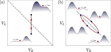
Figure 1: Single-electron pumping. (a) Non-adiabatic charge pumping can be achieved by modulating a single gate voltage periodically in time as indicated by the red line. In this case, mainly the left barrier of the gate-defined potential is periodically modulated as illustrated by the insets. The dashed line separates the stable charge configurations of the island (0 or 1 electrons). (b) Adiabatic pumping can be achieved by slowly modulating both gate voltages periodically in time as indicated by the positively-oriented contour in red. The insets illustrate how both barriers are periodically modulated.

II Quantized charge pumping

The Floquet theory that we develop below is applicable to a large class of open quantum systems that exchange particles (or heat) with external reservoirs and whose dynamics can be described by a Markovian (generalized) master equation. To be specific, we here consider periodically-driven single-electron pumps that ideally transfer one electron from a source electrode to a collector in every single operation cycle. A charge pump consists of a nano-scale island whose dynamics is governed by the master equation

$$\frac{d}{dt}|P(t)\rangle=\mathbf{L}(t)|P(t)\rangle,$$ (1)

where the vector $|P(t)\rangle=[p_{0}(t),p_{1}(t),p_{2}(t),\ldots]^{T}$ contains the probabilities for the island to be occupied by $0,1,2,...$ electrons. The rate matrix $\mathbf{L}(t)=\mathbf{L}(t+\mathcal{T})$ describes the transitions between different charge states of the island, and $\mathcal{T}$ is the period of the external drive. At all times, the product of the tunneling amplitudes to the source and the collector is kept so small that co-tunneling processes can safely be ignored and we may consider sequential single-electron tunneling only.

To investigate the pumped current, we resolve the probability vector $|P(t)\rangle=\sum_{n}|P(n,t)\rangle$ with respect to the number of electrons $n$ that have been transferred during the time-span $[0,t]$ Plenio and Knight (1998). The charge transfer statistics can then be expressed as $P(n,t)=\langle 1|P(n,t)\rangle$ with all entries of the vector $\langle 1|$ being $1$. We also write the rate matrix as $\mathbf{L}(t)=\mathbf{L}_{0}(t)+\mathbf{J}_{+}(t)+\mathbf{J}_{-}(t)$ with $\mathbf{J}_{\pm}(t)$ describing charge transfers to and from the collector Benito et al. (2016). The equations of motion, $\frac{d}{dt}|P(n,t)\rangle=\mathbf{L}_{0}(t)|P(n,t)\rangle+\mathbf{J}_{+}(t)|P(n-1,t)\rangle+\mathbf{J}_{-}(t)|P(n+1,t)\rangle$, are decoupled by introducing the counting field $\chi$ via the definition $|P(\chi,t)\rangle\equiv\sum_{n}|P(n,t)\rangle e^{in\chi}$. We then arrive at a modified master equation for $|P(\chi,t)\rangle$

$$\frac{d}{dt}|P(\chi,t)\rangle=\mathbf{L}(\chi,t)|P(\chi,t)\rangle$$ (2)

with $\mathbf{L}(\chi,t)=\mathbf{L}(t)+(e^{i\chi}-1)\mathbf{J}_{+}(t)+(e^{-i\chi}-1)\mathbf{J}_{-}(t)$. Formally, the solution $|P(\chi,t)\rangle=\mathbf{U}(\chi,t)|P(\chi,0)\rangle$ is given by the time-ordered exponential $\mathbf{U}(\chi,t)=\hat{T}\{e^{\int_{0}^{t}dt^{\prime}\mathbf{L}(\chi,t^{\prime})}\}$ Pistolesi (2004); Potanina and Flindt (2017). The moments of the pumped charge $n$ then follow as $\langle n^{m}\rangle(t)=\partial_{i\chi}^{m}\mathcal{M}(\chi,t)|_{\chi=0}$, where $\mathcal{M}(\chi,t)\equiv\sum_{n}P(n,t)e^{in\chi}=\langle 1|\mathbf{U}(\chi,t)|P(\chi,0)\rangle$ is the moment generation function. Similarly, the cumulant generating function $\mathcal{S}(\chi,t)\equiv\ln\mathcal{M}(\chi,t)$ delivers the cumulants as $\langle\!\langle n^{m}\rangle\!\rangle(t)=\partial_{i\chi}^{m}\mathcal{S}(\chi,t)|_{\chi=0}$. Below, we focus on the first two cumulants, namely the mean $\langle\!\langle n\rangle\!\rangle=\langle n\rangle$ and the variance $\langle\!\langle n^{2}\rangle\!\rangle=\langle n^{2}\rangle-\langle n\rangle^{2}$, although higher cumulants can easily be obtained with little added effort.

III Floquet theory

We now make use of the periodicity of the drive. Building on the Floquet theorem Bukov et al. (2015), the time-evolution operator can be expressed as $\mathbf{U}(\chi,t)=\sum_{i}e^{\lambda_{i}(\chi)t}|p_{i}(\chi,t)\rangle\!\langle p_{i}(\chi,0)|$, where $|p_{i}(\chi,t)\rangle=|p_{i}(\chi,t+\mathcal{T})\rangle$ solves the Floquet eigenvalue problem

$$\left[\mathbf{L}(\chi,t)-\frac{d}{dt}\right]|p_{i}(\chi,t)\rangle=\lambda_{i}(\chi)|p_{i}(\chi,t)\rangle.$$ (3)

We then obtain $\mathcal{S}(\chi,t)=\ln{\sum_{i}e^{\lambda_{i}(\chi)t}\langle 1|p_{i}(\chi,t)\rangle}$ and immediately see that the charge transfer statistics after many periods $\mathcal{N}\gg 1$ is fully encoded in the Floquet eigenvalue $\phi(\chi)\equiv\max\limits_{i}\left[\lambda_{i}(\chi)\right]$ with the largest real-part

$$\mathcal{S}(\chi,\mathcal{N}\mathcal{T})\simeq\mathcal{N}\mathcal{T}\phi(\chi).$$ (4)

Generally, however, it is a daunting task to determine $\phi(\chi)$ and its dependence on the counting field. Nevertheless, as we go on to show, the eigenvalue can be found perturbatively in the frequency or the period of the drive.

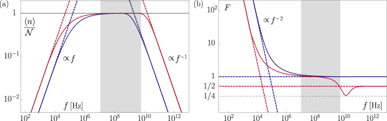
Figure 2: Single-parameter pump. (a) Average pumped charge per period as a function of the driving frequency $f$. The solid lines are numerical results, while the dashed lines are the low and high-frequency expansions. The red line is obtained with driving parameters that minimize the Fano factor at high frequencies. The shaded area indicates the quantized-current plateau for the optimized driving parameters. The system parameters are $C=10$ aF, $G=1.0\times 10^{-4}$ $\Omega^{-1}$, $T=0.2$ K, and $\Gamma=G/4C=2.5\times 10^{12}$ s^-1. The driving parameters are $V_{L}^{0}=4$ mV (blue), $24$ mV (red), $V_{R}^{0}=0.8$ mV, $V_{s}=5$ $\mu$V, $\mathcal{N}_{g}=0.2$. (b) The Fano factor $F=\langle\!\langle n^{2}\rangle\!\rangle/\langle n\rangle$ of the pumped charge as a function of the driving frequency.

IV Adiabatic expansion

We first evaluate the Floquet eigenvalue $\phi(\chi)$ and the corresponding eigenvector, denoted as $|p(\chi,t)\rangle$, perturbatively in the driving frequency. In the adiabatic expansion, we treat the time-derivative $-\frac{d}{dt}$ in Eq. (3) as the perturbation Cavina et al. (2017). Our adiabatic expansion can be formulated in terms of the instantaneous eigenvalue of $\mathbf{L}(\chi,t)$ with the largest real-part $\lambda^{(0)}(\chi,t)$ and the corresponding eigenvectors $\langle p^{(0)}(\chi,t)|$ and $|p^{(0)}(\chi,t)\rangle$. To begin with, we find from Eq. (3)

$$\phi(\chi)=\phi^{(0)}(\chi)-\int_{0}^{\mathcal{T}}\frac{dt}{\mathcal{T}}\langle p^{(0)}(\chi,t)|\frac{d}{dt}|p(\chi,t)\rangle,$$ (5)

where $\phi^{(0)}(\chi)=\int_{0}^{\mathcal{T}}\frac{dt}{\mathcal{T}}\lambda^{(0)}(\chi,t)$ is the average of the instantaneous eigenvalue. Without a voltage bias, the contribution to the mean current from $\phi^{(0)}(\chi)$ vanishes and the noise can be related to the conductance according to the fluctuation-dissipation theorem Blanter and Büttiker (2000). To proceed to higher orders, we expand the eigenvalue and eigenvector in the perturbation as $\phi(\chi)=\sum_{k=0}^{\infty}\phi^{(k)}(\chi)$ and $|p(\chi,t)\rangle=\sum_{k=0}^{\infty}|p^{(k)}(\chi,t)\rangle$ and collect terms of the same order in Eq. (5). To first order, we find $\phi^{(1)}(\chi)=-\int_{0}^{\mathcal{T}}\frac{dt}{\mathcal{T}}\langle p^{(0)}(\chi,t)|\frac{d}{dt}|p^{(0)}(\chi,t)\rangle$ as previously established within a different framework Sinitsyn and Nemenman (2007a, b); Ren et al. (2010); Goswami et al. (2016). For a device controlled by a single parameter, this term vanishes as we discuss below. To second order, we find

$$\phi^{(2)}(\chi)=-\int_{0}^{\mathcal{T}}\frac{dt}{\mathcal{T}}\langle p^{(0)}(\chi,t)|\frac{d}{dt}\mathbf{R}(\chi,t)\frac{d}{dt}|p^{(0)}(\chi,t)\rangle$$ (6)

having used $|p^{(1)}(\chi,t)\rangle=\mathbf{R}(\chi,t)\frac{d}{dt}|p^{(0)}(\chi,t)\rangle$ as in standard perturbation theory, where $\mathbf{R}(\chi,t)$ is the pseudo-inverse of $\mathbf{L}(\chi,t)-\lambda^{(0)}(\chi,t)$ Flindt et al. (2010). Equation (6) is important as it allows us to evaluate the charge transfer statistics for single-parameter pumps to first non-trivial order in the driving frequency. Before demonstrating its usefulness with specific applications, we discuss our high-frequency expansion of the cumulant generating function.

V High-frequency expansion

The high-frequency expansion proceeds differently. Here, we write the time-evolution operator as $\mathbf{U}(\chi,\mathcal{N}\mathcal{T})=[\mathbf{U}(\chi,\mathcal{T})]^{\mathcal{N}}:=e^{\mathcal{N}\mathcal{T}\mathbf{L}_{F}(\chi)}$ and identify the Floquet eigenvalue $\phi(\chi)$ as the eigenvalue of $\mathbf{L}_{F}(\chi)$ with the largest real-part. Using a Floquet-Magnus expansion $\mathbf{L}_{F}(\chi)=\sum_{k=0}^{\infty}\mathbb{L}^{(k)}(\chi)$, we can then evaluate $\phi(\chi)$ perturbatively in the period. The first two terms read $\mathbb{L}^{(0)}(\chi)=\int_{0}^{\mathcal{T}}\frac{dt}{\mathcal{T}}\mathbf{L}(\chi,t)$ and $\mathbb{L}^{(1)}(\chi)=\int_{0}^{\mathcal{T}}\frac{dt}{2}\int_{0}^{t}\frac{dt^{\prime}}{\mathcal{T}}[\mathbf{L}(\chi,t),\mathbf{L}(\chi,t^{\prime})]$ Blanes et al. (2009); Bukov et al. (2015); Kuwahara et al. (2016). In the high-frequency expansion $\phi(\chi)=\sum_{k=0}^{\infty}\varphi^{(k)}(\chi)$, the first term $\varphi^{(0)}(\chi)$ is given by the eigenvalue of $\mathbb{L}^{(0)}(\chi)$ with the largest real-part. Denoting the corresponding eigenvectors by $\langle\mathbb{p}^{(0)}(\chi)|$ and $|\mathbb{p}^{(0)}(\chi)\rangle$, the next term becomes $\varphi^{(1)}(\chi)=\langle\mathbb{p}^{(0)}(\chi)|\mathbb{L}^{(1)}(\chi)|\mathbb{p}^{(0)}(\chi)\rangle.$ Thus, with the eigenvectors of $\mathbb{L}^{(0)}(\chi)$ at hand, we can evaluate the charge transfer statistics perturbatively in the period.

VI Single-electron pump

We can now analyze a charge pump which is similar to those from recent experiments Giblin et al. (2012); Ono and Takahashi (2003); Fujiwara et al. (2008); Jehl et al. (2013); Yamahata et al. (2014); Rossi et al. (2014); Blumenthal et al. (2007); Giblin et al. (2010); Kataoka et al. (2011); Fricke et al. (2014); Ubbelohde et al. (2015); Stein et al. (2015); Yamahata et al. (2016); Ahn et al. (2017); Zhao et al. (2017). The pump consists of a metallic island operated in the Coulomb-blockade regime, where the island is either empty or occupied by one electron. The rate matrix then takes the simple form

$$\mathbf{L}(\chi,t)=\left(\begin{array}[]{ll}-\Gamma^{+}_{L}(t)-\Gamma^{+}_{R}(t)&\Gamma^{-}_{L}(t)+\Gamma^{-}_{R}(t)e^{i\chi}\\ \\ \Gamma^{+}_{L}(t)+\Gamma^{+}_{R}(t)e^{-i\chi}&-\Gamma^{-}_{L}(t)-\Gamma^{-}_{R}(t)\end{array}\right),$$

where $\Gamma_{\alpha}^{\pm}(t)=\frac{G_{\alpha}(t)}{q^{2}}\frac{\pm\Delta E(t)}{\exp[\pm\beta\Delta E(t)]-1}$ is the rate at which tunneling occurs between the island and the leads, changing the occupation by $\pm 1$ electron with charge $-q$. No voltage bias is applied, and $\beta=1/k_{B}T$ is the inverse temperature. The change of the electrostatic energy due to the addition of an electron reads $\Delta E(t)=-E_{\mathrm{c}}[\mathcal{N}_{g}+2\{C_{L}V_{L}(t)+C_{R}V_{R}(t)\}/q]$, where $C_{\alpha}$ are the gate capacitances, $E_{\mathrm{c}}=q^{2}/2(C_{L}+C_{R})$ is the charging energy, and the offset $\mathcal{N}_{g}$ can be controlled with a back-gate Pekola et al. (2013). The barrier conductances depend exponentially on the gate voltages, $G_{\alpha}(t)=G_{\alpha}\exp[V_{\alpha}(t)/V_{s}]$, where $V_{s}$ is known as the sub-threshold slope Jehl et al. (2013).

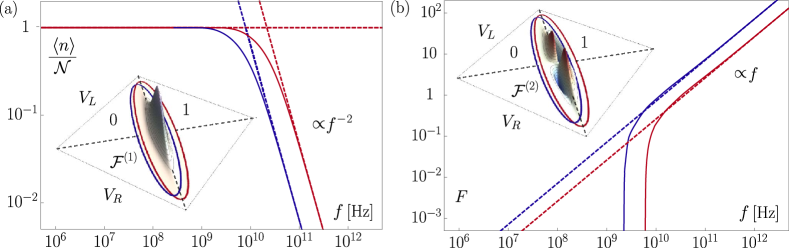
Figure 3: Pumped charge (a) and the Fano factor (b) for the two-parameter pump. The driving protocol $\textbf{V}(t)=-V^{0}[\cos(2\pi ft)+\alpha,\cos(2\pi ft+\vartheta)+\alpha]^{T}$ is shown together with the Berry curvatures $\mathcal{F}^{(j)}$ in the insets, where the stable charge configuration of the island is also indicated (0 or 1 electrons). The solid lines are numerical results, while the dashed lines are the low and high-frequency approximations. The system parameters are given in Fig. 2. The driving parameters are $V^{0}=8$ mV, $\vartheta=1.02\pi$, $\mathcal{N}_{g}=2$, and $\alpha=1.01$ (blue), $\alpha=\mathcal{N}_{g}/2=1$ (red).

VII Single-parameter pumping

We first consider a single-parameter pump, where the right gate voltage is kept constant, $V_{R}(t)=-V_{R}^{0}$, while the left one is subject to the harmonic drive $V_{L}(t)=-V_{L}^{0}\left[\cos(2\pi ft)+1\right]$. For low frequencies, the average of the pumped charge is obtained from Eq. (6). At low temperatures, where the tunneling rates $\Gamma^{-}_{L}(t)\simeq\Gamma^{+}_{R}(t)\simeq 0$ are small, we find

$$\frac{\langle n\rangle}{\mathcal{N}}\simeq f\int_{0}^{1}ds\frac{\left[\Gamma_{L}^{+}(s)\right]^{4}\left(\frac{d}{ds}[\Gamma^{-}_{R}(s)/\Gamma^{+}_{L}(s)]\right)^{2}}{\left[\Gamma^{+}_{L}(s)+\Gamma^{-}_{R}(s)\right]^{5}},$$ (7)

having introduced the dimensionless time $s=ft$ to show that the pumped charge is proportional to the driving frequency $f$. We also find that the variance can be expressed as $\langle\!\langle n^{2}\rangle\!\rangle/\mathcal{N}=2k_{B}T\int_{0}^{1}dsG(s)/q^{2}f$ in terms of the instantaneous linear conductance $G(t)$ in accordance with the fluctuation-dissipation theorem. Combined with Eq. (7), we see that the Fano factor $F=\langle\!\langle n^{2}\rangle\!\rangle/\langle n\rangle$ must be proportional to $f^{-2}$ at low frequencies.

For high frequencies, we find the pumped charge from the first term in the Floquet-Magnus expansion,

$$\frac{\langle n\rangle}{\mathcal{N}}\simeq\frac{\Gamma}{f}\left[\frac{qe^{V_{R}^{0}/V_{s}}}{2C(V_{L}^{0}+V_{R}^{0})-q\mathcal{N}_{g}}+\frac{q\sqrt{2\pi V_{L}^{0}/V_{s}}}{q\mathcal{N}_{g}-2CV_{R}^{0}}\right]^{-1}.$$ (8)

Here, we have taken $C_{L}=C_{R}=C$ and $G_{L}=G_{R}=G$ with $\Gamma=G/4C$ being an inverse $RC$-time. The gate voltage must change considerably compared to the sub-threshold slope to open and close the left barrier, while being smaller than the charging energy, so that $2CV_{R}^{0}<q\mathcal{N}_{g}<2C(V_{L}^{0}+V_{R}^{0})$. The Fano factor thus becomes

$$F\simeq\frac{e^{-\frac{2V_{R}^{0}}{V_{s}}}[2C(V_{L}^{0}+V_{R}^{0})-q\mathcal{N}_{g}]^{2}+\frac{V_{s}}{2\pi V_{L}^{0}}(q\mathcal{N}_{g}-2CV_{R}^{0})^{2}}{\left(e^{-\frac{V_{R}^{0}}{V_{s}}}[2C(V_{L}^{0}+V_{R}^{0})-q\mathcal{N}_{g}]+\sqrt{\frac{V_{s}}{2\pi V_{L}^{0}}}(q\mathcal{N}_{g}-2CV_{R}^{0})\right)^{2}}.$$ (9)

Figure 2 shows numerical results for the pumped charge and the Fano factor together with our approximations. The blue curves illustrate the good agreement between the numerics and our perturbative results. With Eqs. (7,8) we quantitatively explain the low and high frequency dependence of the pumped charge, which previously has been observed in numerical calculations Kaestner et al. (2008). Moreover, our results allow us to optimize the driving parameters. By inspecting Eq. (9), we see that the Fano factor takes the minimal value of $1/2$, if $e^{-\frac{V_{R}^{0}}{V_{s}}}[2C(V_{L}^{0}+V_{R}^{0})-q\mathcal{N}_{g}]=\sqrt{\frac{V_{s}}{2\pi V_{L}^{0}}}(q\mathcal{N}_{g}-2CV_{R}^{0})$. We then obtain an optimal ratio of the noise over the pumped charge, which simplifies to $\langle n\rangle/\mathcal{N}\simeq(\Gamma/2f)\sqrt{V_{s}/2\pi V_{L}^{0}}(\mathcal{N}_{g}-2CV_{R}^{0}/q)$. The red lines in Fig. 2 show the results of this optimization. Importantly, compared to the generic blue curve, we obtain an order-of-magnitude increase in the frequencies, for which a quantized current can be produced. Interestingly, the Fano factor dips below $1/2$ at the end of the quantized-current plateau and almost reaches $1/4$, signaling a transition to a new transport regime.

VIII Two-parameter pumping

Next, we modulate both voltages periodically in time, $\textbf{V}(t)=[V_{L}(t),V_{R}(t)]^{T}$. In the adiabatic regime, we can then write $\phi^{(1)}(\chi)=\pm f\int\!\!\!\int_{\mathcal{S}}dV_{L}dV_{R}\mathcal{F}(\chi,\textbf{V})$ by virtue of Stokes’ theorem. Here, the sign is given by the orientation of the contour enclosing the surface $\mathcal{S}$ in the parameter space, and $\mathcal{F}(\chi,\textbf{V})=\left[-\partial_{V_{L}},\partial_{V_{R}}\right]\cdot\langle p^{(0)}(\chi,\textbf{V})|\nabla_{\textbf{V}}|p^{(0)}(\chi,\textbf{V})\rangle$ is a classical analog of the Berry curvature in quantum mechanics Sinitsyn and Nemenman (2007a, b); Ren et al. (2010); Goswami et al. (2016). Clearly, if only one voltage is varied, the surface area vanishes, and $\phi^{(1)}(\chi)=0$. For the pumped charge Pekola et al. (1999); Levinson et al. (2001), we find $\langle n\rangle/\mathcal{N}\simeq\pm\int\!\!\!\int_{\mathcal{S}}dV_{L}dV_{R}\mathcal{F}^{(1)}(\textbf{V})$ with $\mathcal{F}^{(m)}(\textbf{V})=\partial_{i\chi}^{m}\mathcal{F}(\chi,\textbf{V})|_{\chi=0}$ and

$$\mathcal{F}^{(1)}=\frac{q\beta e^{(V_{L}+V_{R})/V_{s}}}{4V_{s}\left(e^{V_{L}/V_{s}}\!+\!e^{V_{R}/V_{s}}\right)^{2}\cosh^{2}\left(\beta\Delta E/2\right)}$$ (10)

as shown in Fig. 3a. For the variance $\langle\!\langle n^{2}\rangle\!\rangle/\mathcal{N}\simeq 2k_{B}T\int_{0}^{1}dsG(s)/q^{2}f\pm\int\!\!\!\int_{\mathcal{S}}dV_{L}dV_{R}\mathcal{F}^{(2)}(\textbf{V})$, we have

$$\mathcal{F}^{(2)}=\frac{q\beta e^{\left(V_{R}+V_{L}\right)/V_{s}}\left(e^{V_{R}/V_{s}}\!-\!e^{V_{L}/V_{s}}\right)\sinh^{4}(\beta\Delta E/2)}{32V_{s}\left(e^{V_{R}/V_{s}}\!+\!e^{V_{L}/V_{s}}\right)^{3}\sinh^{3}(\beta\Delta E)}$$ (11)

as shown in Fig. 3b. We can now position our contour, so that the pumped charge is maximized, and the noise is minimized. To this end, we exploit the symmetry $\mathcal{F}^{(j)}(V_{L},V_{R})=\mathcal{F}^{(j)}(-V_{C}-V_{L},-V_{C}-V_{R})$, $j=1,2$, about the point $(-V_{C}/2,-V_{C}/2)$ with $V_{C}=q/2C$, together with the symmetry $\mathcal{F}^{(j)}(V_{L},V_{R})=(-1)^{j-1}\mathcal{F}^{(j)}(V_{R},V_{L})$ across the line $V_{L}=V_{R}$. Specifically, for a fixed shape of the contour, the contribution to the variance vanishes, if the contour is placed symmetrically across the line $V_{L}=V_{R}$. In that case, the noise is due to equilibrium fluctuations only. Moreover, the pumped charge is maximized, if the contour is also symmetric about the point $(-V_{C}/2,-V_{C}/2)$.

Figure 3 shows the pumped charge and the Fano factor for the driving protocols indicated in the insets together with the Berry curvatures. As in the experiments of Refs. Jehl et al. (2013); Ono and Takahashi (2003), we consider elliptic contours in the parameter space. Both the red and the blue ellipse minimize the noise, while only the red one also maximizes the pumped charge. In the high-frequency regime, the pumped charge $\langle n\rangle/\mathcal{N}\simeq\mathcal{T}\partial_{i\chi}\varphi^{(1)}(\chi)|_{\chi=0}$ decreases as $1/f^{2}$, since there is no contribution from $\varphi^{(0)}(\chi)$ without a voltage bias. The variance, by contrast, is dominated by thermal fluctuations described by $\varphi^{(0)}(\chi)$. We then have $\langle\!\langle n^{2}\rangle\!\rangle/\mathcal{N}\simeq\mathcal{T}\partial^{2}_{i\chi}\varphi^{(0)}(\chi)|_{\chi=0}$, implying that the Fano factor is proportional to the frequency. These conclusions are supported by our numerical results in Fig. 3. At low frequencies, the Fano factor is very small (not visible in the figure) and inversely proportional to the frequency. Importantly, from our high-frequency expansion, we get a good estimate of the breakdown frequency for which a quantized current can no longer be generated.

IX Conclusions

We have employed full counting statistics techniques to optimize the operation of charge pumps. To this end, we have used Floquet theory to evaluate the cumulant generating function for the distribution of pumped charge perturbatively in the frequency or the period of the drive. For the device optimization, we have focused on the average and the variance (noise) of the pumped charge, but higher cumulants, or even the large-deviation statistics, can be obtained along the same lines with little added effort. Our theoretical framework covers a wide range of driving frequencies, in the adiabatic regime and for fast driving, and it is useful for practical device optimization. The advances reported here were made possible due to the progress made in theories of driven systems. Our work demonstrates that full counting statistics is a powerful tool to optimize charge pumps, and our predictions may be confirmed in future experiments.