Degrees of Freedom and Model Selection for $k$-means Clustering

Abstract

This paper investigates the model degrees of freedom in $k$-means clustering. An extension of Stein’s lemma provides an expression for the effective degrees of freedom in the $k$-means model. Approximating the degrees of freedom in practice requires simplifications of this expression, however empirical studies evince the appropriateness of our proposed approach. The practical relevance of this new degrees of freedom formulation for $k$-means is demonstrated through model selection using the Bayesian Information Criterion. The reliability of this method is validated through experiments on simulated data as well as on a large collection of publicly available benchmark data sets from diverse application areas. Comparisons with popular existing techniques indicate that this approach is extremely competitive for selecting high quality clustering solutions. Code to implement the proposed approach is available in the form of an R package from https://github.com/DavidHofmeyr/edfkmeans.

Keywords: clustering; $k$-means; model selection; cluster number determination; degrees of freedom; Bayesian Information Criterion; penalised likelihood

1 Introduction

Degrees of freedom arise explicitly in model selection, as a way of accounting for the bias in the model log-likelihood for estimating generalisation performance (Akaike, 1998, Akaike Information Criterion, AIC) and, indirectly, Bayes factors (Schwarz et al., 1978, Bayesian Information Criterion, BIC). In particular, degrees of freedom account for the complexity, or flexibility of a model by measuring its effective number of parameters. In the context of clustering, model flexibility is varied primarily by different choices of $k$, the number of clusters. In $k$-means, clusters are associated with compact collections of points arising around a set of cluster centroids. The optimal centroids are those which minimise the sum of squared distances between each point and its assigned centroid. Using the squared distance connects the $k$-means objective with the log-likelihood of a simple Gaussian Mixture Model (GMM). Pairing elements of the GMM log-likelihood with AIC and BIC type penalties, based on the number of explicitly estimated parameters, has motivated multiple model selection methods for $k$-means (Manning et al., 2008; Ramsey et al., 2008; Pelleg et al., 2000). However, it has been observed that these approaches can lead to substantial over-estimation of the number of clusters (Hamerly and Elkan, 2004).

We argue that these simple penalties are inappropriate, and do not account for the entire complexity of the model, and investigate more rigorously the degrees of freedom in the $k$-means model. The proposed formulation depends not only on the explicit dimension of the model, but also accounts for the uncertainty in the cluster assignments. This is intuitively appealing, as it allows the degrees of freedom to incorporate the difficulty of the clustering problem, which cannot be captured solely by the model dimension. This formulation draws on the work of Tibshirani (2015), and is the first application, of which we are aware, of this approach to the problem of clustering. We validate the proposed formulation by applying it within the BIC to perform model selection for $k$-means. The approach is found to be extremely competitive with the state-of-the-art on a very large collection of benchmark data sets.

The remaining paper is organised as follows. In Section 2 we discuss the $k$-means model explicitly, and consider its degrees of freedom. We also provide details for how we approximate the degrees of freedom practically. Section 3 describes our approach for model selection based on the Bayesian Information Criterion and using these approximated degrees of freedom. Section 4 documents the results from a thorough simulation study as well as comparisons between the proposed approach and popular existing methods on simulated data, as well as on a very large collection of publicly available benchmark data sets. Finally, we give some concluding remarks in Section 5.

2 Degrees of Freedom in the $k$-means Model

From a probabilistic perspective, the standard modelling assumptions for $k$-means are that the data arose from a $k$ component Gaussian mixture in $d$ dimensions with equal isotropic covariance matrix, $\sigma^{2}I$, and either equal mixing proportions (Manning et al., 2008; Celeux and Govaert, 1992) or sufficiently small $\sigma$ (Jiang et al., 2012). In this case, and with a slight abuse of notation, one may in general write the likelihood for the data, given model $\mathcal{M}$, which we assume to include all parameters of the underlying distribution which are being estimated, as

$$\ell(\mathbf{X}|\mathcal{M}) =\sum_{i=1}^{n}\log\left(\sum_{j=1}^{k}\pi_{ij}\frac{1}{(2\pi\sigma^{2})^{d/2}}\exp\left(-\frac{||\mathbf{X}_{i\_}-\boldsymbol{\mu}_{j}||^{2}}{2\sigma^{2}}\right)\right).$$

Here $\boldsymbol{\mu}_{1},...,\boldsymbol{\mu}_{k}\in\mathbb{R}^{d}$ are the component means, $\pi_{ij}$ is the probability that the $i$-th datum arises from the $j$-th component, and the subscript “$i\_$” is used to denote the $i$-th row of a matrix. The terms $\pi_{ij}$ are usually assumed equal for fixed $j$, and have been used to represent mixing proportions (Manning et al., 2008). Popular formulations of the $k$-means likelihood (Manning et al., 2008; Ramsey et al., 2008; Pelleg et al., 2000) use the so-called classification likelihood (Fraley and Raftery, 2002), which treats the cluster assignments as true class labels. For example, a simple BIC formulation has been expressed, up to an additive constant, as (Ramsey et al., 2008)

$$\frac{1}{\sigma^{2}}\sum_{i=1}^{n}\min_{j\in\{1,...,k\}}||\mathbf{X}_{i\_}-\hat{\boldsymbol{\mu}}_{j}||^{2}+\log(n)kd.$$ (1)

Here only the means are assumed part of the estimation, and hence the model dimension is $kd$, for $k$ clusters. There is a fundamental mismatch in formulations such as this, however, including those in Manning et al. (2008); Ramsey et al. (2008); Pelleg et al. (2000), between the log-likelihood component and the bias correction term. Specifically, by using the classification likelihood the assumption is that the model is also estimating the assignments of data to clusters. However, without incorporating this added estimation into the model degrees of freedom, the bias of the log-likelihood for estimating generalisation error, and Bayes factors, is severely under-estimated.

In this work a modified formulation is considered which incorporates the cluster assignment into the modelling procedure. We find it convenient to assume that the data matrix $\mathbf{X}$ has been generated as,

$$\mathbf{X}={{\upmu}}+\mathbf{E},$$ (2)

where the mean matrix ${{\upmu}}\in\mathbb{R}^{n\times d}$ is assumed to have $k$ unique rows and the elements of $\mathbf{E}\in\mathbb{R}^{n\times d}$ are independent realisations from a $N(0,\sigma^{2})$ distribution. Notice that in this case the log-likelihood may be written as,

$$\ell(\mathbf{X}|{{\upmu}},\sigma) =\sum_{i=1}^{n}\sum_{j=1}^{d}\log\left(\frac{1}{\sqrt{2\pi}\sigma}\exp\left(-\frac{(\mathbf{X}_{i,j}-{{\upmu}}_{i,j})^{2}}{2\sigma^{2}}\right)\right)$$

$$=-\frac{1}{2\sigma^{2}}\sum_{i=1}^{n}\sum_{j=1}^{n}(\mathbf{X}_{i,j}-{{\upmu}}_{i,j})^{2}-nd\log(\sigma)+K,$$

for constant $K$ independent of $\sigma$ and ${{\upmu}}$. Note that in this formulation the assignment of data (rows of $\mathbf{X}$) to mixture components is captured implicitly by the $k$ distinct rows of ${{\upmu}}$. Also notice that if $\sigma$ is assumed fixed then this is essentially equivalent (up to an additive constant) to the likelihood term in the BIC formulation in (1) above.

For this formulation it is possible to consider estimating pointwise the elements of ${{\upmu}}$, under the constraint of having $k$ unique rows, using a modelling procedure $\mathcal{M}:\mathbb{R}^{n\times d}\to\mathbb{R}^{n\times d}$, defined as

$$\mathcal{M}(\mathbf{X})_{i,j} =\hat{{{\upmu}}}_{c(i),j}$$ (3)

$$\hat{{{\upmu}}} =\operatorname{\mathrm{argmin}}_{\mathbf{M}\in\mathbb{R}^{k\times d}}\sum_{i=1}^{n}\min_{l\in\{1,...,k\}}||\mathbf{X}_{i\_}-\mathbf{M}_{l\_}||^{2}$$ (4)

$$c(i) =\operatorname{\mathrm{argmin}}_{l\in\{1,...,k\}}||\mathbf{X}_{i\_}-\hat{{{\upmu}}}_{l\_}||^{2}.$$ (5)

The matrix $\hat{{{\upmu}}}\in\mathbb{R}^{k\times d}$ estimates the unique rows of ${{\upmu}}$, and provides an approximation of the maximum likelihood solution under Eq (2). The indices $c(i),i=1,...,n$ indicate the assignments of the data (rows of $\mathbf{X}$) to the different clusters’ means (rows of $\hat{}{{\upmu}}$). With this formulation we are able address the estimation of the “effective degrees of freedom” (Efron, 1986), given by

$$\mathrm{df}(\mathcal{M})=\frac{1}{\sigma^{2}}\sum_{i=1}^{n}\sum_{j=1}^{d}\mbox{Cov}(\mathcal{M}(\mathbf{X})_{i,j},\mathbf{X}_{i,j}).$$ (6)

The covariance offers an appealing interpretation in terms of model complexity/flexibility. A more complex model will respond more to variations in the data, in that additional flexibility will allow the model to attempt to “explain” this variation. The covariance between its fitted values and the data will therefore be higher. On the other hand, an inflexible model will, by definition, vary less due to changes in the observations. Furthermore in numerous simple Gaussian error models there is an exact equality between this covariance and the model dimension. The remainder of this section is concerned with obtaining an appropriate approximation of the effective degrees of freedom for the $k$-means model. The following two lemmas are useful for obtaining such an estimate.

Lemma 1

Let $\mathbf{X}={{\upmu}}+\mathbf{E}\in\mathbb{R}^{n\times d}$, with ${{\upmu}}$ fixed and $\mathbf{E}_{i,j}\sim N(0,\sigma^{2})$ with $\mathbf{E}_{i,j},\mathbf{E}_{k,l}$ independent for all $(i,j)\not=(l,k)$. Let $f:\mathbb{R}^{n\times d}\to\mathbb{R}^{n\times d}$ satisfy the following condition. For all $\mathbf{W}\in\mathbb{R}^{n\times d}$ and each $i,j$, there exists a finite set $\mathcal{D}^{\mathbf{W}}_{i,j}=\bigcup_{l=1}^{q}\{\delta_{l}\}$ s.t. $f$, viewed as a univariate function by keeping all other elements of $\mathbf{W}$, $\{\mathbf{W}_{k,l}\}_{(k,l)\not=(i,j)}$, fixed, is Lipschitz on each of $(-\infty,\delta_{1}),(\delta_{1},\delta_{2}),...,(\delta_{q-1},\delta_{q})$, and $(\delta_{q},\infty)$. Then for each $i,j$, the quantity $\frac{1}{\sigma^{2}}Cov(f(\mathbf{X})_{i,j},\mathbf{X}_{i,j})$ is equal to

$$E\left[\frac{\partial}{\partial\mathbf{X}_{i,j}}f(\mathbf{X})_{i,j}\right]+\frac{1}{\sigma}E\Bigg{[}\sum_{\delta:\mathbf{X}_{i,j}+\delta\in\mathcal{D}_{i,j}^{\mathbf{X}}}\phi\left(\frac{\mathbf{X}_{i,j}+\delta-{{\upmu}}_{i,j}}{\sigma}\right)\lim_{\gamma\downarrow\uparrow\delta}f(\mathbf{X}+\gamma\mathbf{e}_{i,j})_{i,j}\Bigg{]},$$ (7)

provided the second term on the right hand side exists. Here $\phi(x)=(2\pi)^{-1/2}\exp(-x^{2}/2)$ is the Gaussian density function; $\mathbf{e}_{i,j}\in\mathbb{R}^{n\times d}$ has zero entries except in the $i,j$-th position, where it takes the value one; and

$$\lim_{\gamma\downarrow\uparrow\delta}f(\mathbf{X}+\gamma\mathbf{e}_{i,j})=\lim_{\gamma\downarrow\delta}f(\mathbf{X}+\gamma\mathbf{e}_{i,j})-\lim_{\gamma\uparrow\delta}f(\mathbf{X}+\gamma\mathbf{e}_{i,j}).$$

is the size of the discontinuity at $\delta$.

This result is very similar to (Tibshirani, 2015, Lemma 5), where the regression context is considered. Our proof is given in the appendix. The first term in (7) comes from Stein’s influential result (Stein, 1981, Lemma 2) for determining the risk in the estimation of the mean of a Gaussian random variable using a smooth model. Due to the discontinuities in the $k$-means model, which occur at points where the cluster assignments of some of the data change, the additional covariance at the discontinuity points needs to be accounted for. Consider an $\mathbf{X}$ which is close to a point of discontinuity with respect to the $i,j$-th entry. Conditional on the fact that $\mathbf{X}$ is close to such a point, $f(\mathbf{X})_{i,j}$ takes values approximately equal to the left and right limits, depending on whether $\mathbf{X}_{i,j}$ is below or above the discontinuity respectively. On a small enough scale each happens with roughly equal probability. After taking into account the probability of being close to the discontinuity point, and taking the limit as $\mathbf{X}$ gets arbitrarily close to the discontinuity point, one can arrive at an intuitive justification for the additional term in (7). In the remainder this additional covariance term will be referred to as the excess degrees of freedom.

In the above result the function $f$ may be seen to represent an arbitrary modelling procedure, which takes as argument a data matrix and outputs a matrix of fitted values which represent an estimate of the means of the elements in the data under a Gaussian error model. The next lemma places Lemma 1 in the context of the $k$-means model, where it is verified that the modelling procedure $\mathcal{M}$, described in Eqs. (3)–(5), satisfies the conditions described above. Notice that in this context, the discontinuities in the model (the $\delta$ values in the statement of Lemma 1) correspond with the points at which some of the clustering assignments would change.

Lemma 2

Let $\mathcal{M}:\mathbb{R}^{n\times d}\to\mathbb{R}^{n\times d}$ be defined as

$$\mathcal{M}(\mathbf{W})_{i,j}=\hat{{{\upmu}}}_{c(i),j},$$

where

$$\hat{{{\upmu}}} =\operatorname{\mathrm{argmin}}_{\mathbf{M}\in\mathbb{R}^{k\times d}}\sum_{i=1}^{n}\min_{j\in\{1,...,k\}}||\mathbf{W}_{i\_}-\mathbf{M}_{j\_}||^{2}$$

$$c(i) =\operatorname{\mathrm{argmin}}_{j\in\{1,...,k\}}||\mathbf{W}_{i\_}-\hat{{{\upmu}}}_{j\_}||^{2}.$$

Then $\mathcal{M}$ satisfies the conditions on the function $f$ in the statement of Lemma 1, and moreover if $\mathbf{X}={{\upmu}}+\mathbf{E}\in\mathbb{R}^{n\times d}$, with ${{\upmu}}$ fixed and $\mathbf{E}_{i,j}\sim N(0,\sigma^{2})$ with $\mathbf{E}_{i,j},\mathbf{E}_{k,l}$ independent for all $(i,j)\not=(l,k)$, then

$$E\Bigg{[}\sum_{\delta:\mathbf{X}_{i,j}+\delta\in\mathcal{D}^{\mathbf{X}}_{i,j}}\phi\left(\frac{\mathbf{X}_{i,j}+\delta-{{\upmu}}_{i,j}}{\sigma}\right)\lim_{\gamma\downarrow\uparrow\delta}\mathcal{M}(\mathbf{X}+\gamma\mathbf{e}_{i,j})_{i,j}\Bigg{]}$$

exists and is finite.

One of the most important consequences of (Stein, 1981, Lemma 2), which leads to the first term in (7), is that this term is devoid of any of the parameters of the underlying distribution. An unbiased estimate of this term can be obtained by taking the partial derivatives of the model using the observed data. In the case of $k$-means one arrives at,

$$\frac{\partial\mathcal{M}(\mathbf{X})_{i,j}}{\partial\mathbf{X}_{i,j}}=\frac{\partial\hat{}{{\upmu}}_{c(i),j}}{\partial\mathbf{X}_{i,j}}=\frac{1}{n_{c(i)}},$$

where $n_{c(i)}$ is the number of data assigned to centroid $c(i)$. Therefore,

$$\sum_{i=1}^{n}\sum_{j=1}^{d}\frac{\partial\mathcal{M}(\mathbf{X})_{i,j}}{\partial\mathbf{X}_{i,j}} =\sum_{j=1}^{d}\sum_{l=1}^{k}\sum_{i:c(i)=l}\frac{\partial\mathcal{M}(\mathbf{X})_{i,j}}{\partial\mathbf{X}_{i,j}}$$

$$=\sum_{j=1}^{d}\sum_{l=1}^{k}\sum_{i:c(i)=l}\frac{1}{n_{c(i)}}=\sum_{j=1}^{d}\sum_{l=1}^{k}n_{c(i)}\frac{1}{n_{c(i)}}=kd.$$

The excess degrees of freedom therefore equals the difference between the effective degrees of freedom and the explicit model dimension, i.e., the number of elements in $\hat{}{{\upmu}}$. It may therefore be interpreted as the additional complexity in assigning data to clusters. This is intuitively pleasing in light of the fact that this additional covariance directly accounts for the potential assignment of the data to different clusters, in that these are what result in discontinuities in the model.

2.1 Approximating Excess Degrees of Freedom

The excess degrees of freedom reintroduces the unknown parameters to the degrees of freedom expression. Furthermore, as noted by Tibshirani (2015), it is generally extremely difficult to determine the discontinuity points, making the computation of the excess degrees of freedom very challenging. This perhaps even more so in the case of clustering. Consider the excess degrees of freedom arising from the $i,j$-th entry,

$$\frac{1}{\sigma}E\Bigg{[}\sum_{\delta:\mathbf{X}_{i,j}+\delta\in\mathcal{D}^{\mathbf{X}}_{i,j}}\phi\left(\frac{\mathbf{X}_{i,j}+\delta-{{\upmu}}_{i,j}}{\sigma}\right)\lim_{\gamma\downarrow\uparrow\delta}\mathcal{M}(\mathbf{X}+\gamma\mathbf{e}_{i,j})_{i,j}\Bigg{]}.$$

Assume for now that the model parameters, ${{\upmu}}$ and $\sigma^{2}$, are fixed. We will discuss our approach for accommodating these unknown parameters in the next subsection. Now, recall that the discontinuities $\mathcal{D}^{\mathbf{X}}_{i,j}$ are those $\delta$ at which the assignment of some of the data changes. That is, those $\delta$ for which $\exists m$ s.t.

$$\lim_{\gamma\downarrow\uparrow\delta}\operatorname{\mathrm{argmin}}_{l=1,...,k}||(\mathbf{X}+\gamma\mathbf{e}_{i,j})_{m\_}-\hat{}{{\upmu}}(\mathbf{X}+\gamma\mathbf{e}_{i,j})_{l\_}||\not=0,$$

The fact that discontinuities are determined in terms of the would-be solution, $\hat{}{{\upmu}}(\mathbf{X}+\gamma\mathbf{e}_{i,j})$, rather than the observed solution, $\hat{}{{\upmu}}(\mathbf{X})$, is one of the reasons which make determining the discontinuity points extremely challenging. Here we have made explicit the dependence of the estimated means, $\hat{}{{\upmu}}$, on the data. Indeed, one can construct examples where slight changes in only a single matrix entry can result in reassignments of arbitrarily large subsets of data, resulting in substantial and unpredictable changes in $\hat{}{{\upmu}}$. We are thus led to making some simplifications. First, we only consider discontinuities w.r.t. the $i,j$-th entry arising from reassignments of $\mathbf{X}_{i\_}$, the corresponding datum. This is a necessary simplification which maintains the intuitive interpretation of the excess degrees of freedom as the covariance arising from reassignments of data. Now, consider the value of $\delta$ at which the assignment of $\mathbf{X}_{i\_}$ changes from $c(i)$ to some $l\not=c(i)$. Ignoring all other clusters, we find that $\delta$ satisfies

$$\left\|\mathbf{X}_{i\_}+\delta\mathbf{e}_{j}-\hat{}{{\upmu}}_{c(i)\_}-\frac{\delta}{n_{c(i)}}\mathbf{e}_{j}\right\|^{2} =\left\|\mathbf{X}_{i\_}+\delta\mathbf{e}_{j}-\hat{}{{\upmu}}_{l\_}\right\|^{2},$$ (8)

where $\mathbf{e}_{j}$ is the $j$-th canonical basis vector for $\mathbb{R}^{d}$ and $n_{c(i)}$ is the size of the $c(i)$-th cluster. This is a quadratic equation which can easily be solved. A further simplification is adopted here. Rather than considering the paths of $\mathbf{X}_{i\_}$ through multiple reassignments resulting from varying $\delta$ (which quickly become extremely difficult to calculate), the magnitude and location of a discontinuity at a value $\delta$ is determined as though no reassignments had occurred for values between zero and $\delta$. Since the corresponding values of $\delta$ are generally large, the contributions from the quantities $\phi\left(\frac{\mathbf{X}_{i,j}+\delta-{{\upmu}}_{i,j}}{\sigma}\right)\lim_{\gamma\downarrow\uparrow\delta}\mathcal{M}(\mathbf{X}+\gamma\mathbf{e}_{i,j})_{i,j}$ are generally small, and hence we expect the bias induced by this simplification to be relatively small. The excess degrees of freedom for the $i,j$-th entry is thus approximated using

$$\frac{1}{\sigma}\sum_{l\not=c(i)}\phi\bigg{(}\frac{\mathbf{X}_{i,j}+\delta_{l}-{{\upmu}}_{i,j}}{\sigma}\bigg{)}\lim_{\gamma\downarrow\uparrow\delta_{l}}\mathcal{M}(\mathbf{X}+\gamma\mathbf{e}_{i,j})_{i,j},$$ (9)

where $\delta_{l}$ is the solution to Eq. (8) with smaller magnitude (when a solution exists). To determine the magnitude of the discontinuities observe that when $\delta_{l}<0$, and we assume, as above, that no values $\delta_{l}<\delta<0$ result in a reassignment of $\mathbf{X}_{i\_}$, we have

$$\lim_{\gamma\downarrow\delta_{l}}\mathcal{M}(\mathbf{X}+\gamma\mathbf{e}_{i,j})_{i,j}=\hat{}{{\upmu}}_{c(i),j}+\frac{\delta_{l}}{n_{c(i)}},$$

$$\lim_{\gamma\uparrow\delta_{l}}\mathcal{M}(\mathbf{X}+\gamma\mathbf{e}_{i,j})_{i,j}=\frac{1}{n_{l}+1}\left(n_{l}\hat{}{{\upmu}}_{l,j}+\mathbf{X}_{i,j}+\delta_{l}\right)$$

$$\Rightarrow\lim_{\gamma\downarrow\uparrow\delta_{l}}\mathcal{M}(\mathbf{X}+\gamma\mathbf{e}_{i,j})_{i,j}=\hat{}{{\upmu}}_{c(i),j}-\frac{n_{l}}{n_{l}+1}\hat{}{{\upmu}}_{l,j}-\frac{\mathbf{X}_{i,j}}{n_{l}+1}+\delta_{l}\left(\frac{n_{l}+1-n_{c(i)}}{n_{c(i)}(n_{l}+1)}\right).$$ (10)

If $\delta_{l}>0$ then we simply have the negative of the above.

2.1.1 Selecting Appropriate Values for $\upmu$ and $\sigma^{2}$ for Estimating Degrees of Freedom

The estimate of excess degrees of freedom depends on the values of ${{\upmu}}$ and $\sigma^{2}$. It is tempting to use the apparently natural candidates, based on $\hat{}{{\upmu}}$ and an estimate of the within cluster variance from the model, whose degrees of freedom are being estimated, itself. However, this is inappropriate for the purpose of comparing models. First, notice that the value of $\hat{}{{\upmu}}$ will lead to an underestimation of the terms, $\phi\left(\frac{\mathbf{X}_{i,j}+\delta-{{\upmu}}_{i,j}}{\sigma}\right)$. This is because the values which result in a reassignment of the corresponding datum occur at the boundaries of the estimated clusters; and hence, on average, at the greatest distances from $\hat{}{{\upmu}}$. Furthermore, note that smaller values of $\sigma^{2}$ tend to result in a smaller value of the estimated degrees of freedom, everything else being equal. A model with an over-estimation of $k$ would lead to an underestimation of $\sigma^{2}$, and hence an artifically low estimated degrees of freedom. Such a model would thus be penalised insufficiently, relatively to those with a smaller number of clusters, and hence larger estimate of $\sigma^{2}$.

We have observed that to estimate the degrees of freedom for a model with $k$ clusters, a reasonable approximation can often be obtained by using the estimated parameters from any larger model (i.e., one with a greater number of clusters). In particular, if we now let $\mathcal{M}(\mathbf{X};k)$ be the fitted values from Eqs. (3)–(5), making explicit the number of clusters in the model, then replacing ${{\upmu}}$ and $\sigma$ with $\mathcal{M}(\mathbf{X};k^{\prime})$ and $\sqrt{\frac{1}{nd}\sum_{i=1}^{n}\sum_{j=1}^{d}(\mathbf{X}_{i,j}-\mathcal{M}(\mathbf{X};k^{\prime})_{i,j})^{2}}$ respectively, where $k^{\prime}>k$, provides a reasonable estimate of the degrees of freedom in model $\mathcal{M}(\mathbf{X};k)$. It is interesting that the estimate of degrees of freedom is similar for a large range of values $k^{\prime}$, provided they are greater than $k$. Let’s consider again the terms in the excess degrees of freedom, i.e., terms of the form

$$\frac{1}{\sigma}\phi\left(\frac{\mathbf{X}_{i,j}+\delta-{{\upmu}}_{i,j}}{\sigma}\right)\lim_{\gamma\uparrow\downarrow\delta}\mathcal{M}(\mathbf{X}+\gamma\mathbf{e}_{i,j};k)_{i,j}.$$

Now, notice that the term inside $\phi$ may be seen as having two components, namely $\frac{\mathbf{X}_{i,j}-{{\upmu}}_{i,j}}{\sigma}$ and $\frac{\delta}{\sigma}$. The first of these will tend to be similar for different $k^{\prime}$ when a complementary pair of ${{\upmu}}$ and $\sigma$ is used. Indeed, replacing these with the estimates described above, averaging their squared values over all $i,j$ produces a constant, independent of $k^{\prime}$. Furthermore, notice that, in general, $\delta$ will have the same sign as $\mathbf{X}_{i,j}-{{\upmu}}_{i,j}$, since $\delta$ is the value which causes a change in the assignment of the datum $\mathbf{X}_{i\_}$ from its nearest cluster mean. The term $\phi\left(\frac{\mathbf{X}_{i,j}+\delta-{{\upmu}}_{i,j}}{\sigma}\right)$ will therefore tend to decrease, in general, when considering all pairs $i,j$, as $k^{\prime}$ increases. Conveniently, this decrease is approximately counteracted by the fact that the terms in the excess degrees of freedom include the factor $1/\sigma$, which increases as $k^{\prime}$ increases.

Figure 1 shows the estimated degrees of freedom from $k$-means models obtained from two of the data sets used in our applications. For each of the two data sets we have shown the estimated degrees of freedom for the models with 5, 10 and 15 clusters, and for varying $k^{\prime}$. There is a very clear dip in the plots where $k=k^{\prime}$, caused by underestimation of the degrees of freedom by replacing the unknown parameters with the estimates from the same model. As described above, however, the estimates then become stable for values $k^{\prime}>k$. In practice we simply set $k^{\prime}=k_{max}+1$, where $k_{max}$ is the largest number of clusters under consideration, to estimate the degrees of freedom for all values of $k$.

(a) Wine Data Set

(b) Optical Recognition of Handwritten Digits Data Set

Figure 1: Estimated degrees of freedom for models with $k=5,10$ and 15 clusters, using the estimated parameters from models with a number of clusters, $k^{\prime}$, ranging from 1 to 30. There is a clear dip in the estimates when $k=k^{\prime}$, but the estimates are stable for $k^{\prime}>k$.

2.2 Accuracy of the Approximated Degrees of Freedom

Here we briefly report on a short set of simulations designed to assess the accuracy of the degrees of freedom approximation we have introduced. To begin, we quickly recap our approach. To approximate the degrees of freedom in the model $\mathcal{M}(\mathbf{X};k)$, i.e., the $k$-means solution with $k$ clusters, we first compute, for each $i,j$, those values of $\delta$ at which datum $\mathbf{X}_{i\_}$ would be assigned to another cluster, if shifted in direction $\mathbf{e}_{j}$. That is, for each $l\not=c(i)$, we compute $\delta_{l}^{i,j}$ according to Eq. (8), where we have now introduced explicitly into the notation the indices $i,j$. We then compute the sizes of the model discontinuities at these values of $\delta$, i.e., the values $\lim_{\gamma\downarrow\uparrow\delta^{i,j}_{l}}\mathcal{M}(\mathbf{X}+\gamma\mathbf{e}_{i,j})_{i,j}$, using Eq. (10). Finally, we set

$$\widehat{\mathrm{df}(\mathcal{M}(\mathbf{X};k))}=\frac{1}{\tilde{\sigma}}\sum_{i=1}^{n}\sum_{j=1}^{d}\sum_{l\not=c(i)}\phi\left(\frac{\mathbf{X}_{i,j}+\delta_{l}^{i,j}-\tilde{{{\upmu}}}_{i,j}}{\tilde{\sigma}}\right)\lim_{\gamma\downarrow\uparrow\delta^{i,j}_{l}}\mathcal{M}(\mathbf{X}+\gamma\mathbf{e}_{i,j})_{i,j},$$ (11)

where $\tilde{{{\upmu}}}=\mathcal{M}(\mathbf{X};k^{\prime})$ and $\tilde{\sigma}=\sqrt{\frac{1}{nd}\sum_{i=1}^{n}\sum_{j=1}^{d}(\mathbf{X}_{i,j}-\tilde{{{\upmu}}}_{i,j})^{2}}$ for some $k^{\prime}>k$.

Figure 2 shows the results of our simulation study. Data sets of size 1000 were generated under the modelling assumptions in Eq (2). The number of clusters and dimensions were each set to 5, 10 and 20. The figure shows plots of $k$ against the estimated degrees of freedom based on the above approach, where $k^{\prime}$ was set to $k_{max}+1=31$. The results from 30 replications are shown (——). The plots also show direct empirical estimates of the degrees of freedom obtained by estimating the covariance between the model and the data when sampling from the true distribution (——–). That is, we generate multiple data sets according to Eq (2), apply $k$-means for each value of $k$, and compute the corresponding empirical covariance. To compute the direct estimate of degrees of freedom, this covariance is then simply divided by the true value $\sigma^{2}$. This direct estimate may therefore be seen as our target. For context we also include the plot of $kd$ ($\cdots\cdots$), corresponding to the naïve degrees of freedom equated with the explicit model dimension.

(a) 5 clusters in 5 dimensions

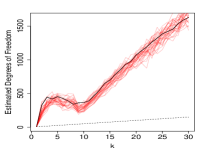
(b) 10 clusters in 5 dimensions

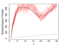
(c) 20 clusters in 5 dimensions

(d) 5 clusters in 10 dimensions

(e) 10 clusters in 10 dimensions

(f) 20 clusters in 10 dimensions

(g) 5 clusters in 20 dimensions

(h) 10 clusters in 20 dimensions

(i) 20 clusters in 20 dimensions

Figure 2: Estimated degrees of freedom computed through (i) direct sampling (——), (ii) proposed method for approximating effective degrees of freedom (——) and (iii) naïve estimate of degrees of freedom ($\cdots\cdots$)

Given the number of simplifications made, and the difficulty of the problem in the abstract, we find the estimation to be very satisfactory in general. The only exceptions apparent from this simple simulation study arose from the 20 dimensional examples, where the proposed method appears to underestimate the degrees of freedom for values of $k$ greater than the true value. Note that from the point of view of model selection, a relatively larger underestimation of the degrees of freedom for a specific value of $k$ will bias the model selection towards that value of $k$. It is therefore this apparent negative bias in the estimated degrees of freedom for higher dimensional cases and for values of $k$ greater than the correct value which we find to be most problematic. We discuss a simple heuristic implemented to mitigate this effect in the next subsection, where we summarise our approach for performing model selection using the estimated degrees of freedom.

3 Choosing $k$ Using the BIC

The Bayesian Information Criterion approximates, up to unnecessary constants, the logarithm of the evidence for a model $\mathcal{M}$, i.e., $P(\mathcal{M}|\mathbf{X})$, using

$$-2\ell(\mathbf{X}|\mathcal{M})+\log(m)\mathrm{df}(\mathcal{M}).$$

Again $\ell(\mathbf{X}|\mathcal{M})$ is the model log-likelihood and here $m$ is the number of independent “residuals” in $\mathbf{X}$. With the modelling assumptions in Eq (2), the BIC for $k$-means is therefore, up to an additive constant,

$$\frac{1}{\sigma^{2}}\sum_{i=1}^{n}\sum_{j=1}^{d}(\mathbf{X}_{i,j}-{{\upmu}}_{i,j})^{2}+nd\log(\sigma^{2})+\log(nd)\mathrm{df}(\mathcal{M}).$$

Setting $\hat{}{{\upmu}}$ here to be equal to $\mathcal{M}(\mathbf{X};k)$, i.e., the matrix of fitted values from the model, and $\hat{\sigma}^{2}=\frac{1}{nd}\sum_{i=1}^{n}\sum_{j=1}^{d}(\mathbf{X}_{i,j}-\hat{}{{\upmu}}_{i,j})^{2}$ to be the corresponding maximum likelihood estimate of the in-cluster variance, the estimated BIC in the $k$-means model with $k$ clusters is therefore, up to an additive constant,

$$nd\log\left(\sum_{i=1}^{n}\sum_{j=1}^{d}(\mathbf{X}_{i,j}-\hat{}{{\upmu}}_{i,j})^{2}\right)+\log(nd)\widehat{\mathrm{df}(\mathcal{M}(\mathbf{X};k))}.$$

Now, we found in the previous section that the proposed approximation method for the model degrees of freedom has the potential to exhibit negative bias for larger values of $d$ and for $k$ greater than the true number of clusters. To mitigate the effect this has on model selection, we select the number of clusters as the smallest value of $k$ which corresponds to a local minimum in the estimated BIC curve, seen as a function of $k$. If no such local minima are present, then we select either $k_{\mathrm{min}}$ or $k_{\mathrm{max}}$; whichever gives the lowest value of the BIC. A similar “first extremum” approach for model selection has also been used by Tibshirani et al. (2001). We also apply a simple local-linear smoothing to the approximated degrees of freedom curves. This mitigates the effect of variation, which is quite pronounced in, e.g., Figure 2 (c) and (f). It also smooths over the short range variation within each estimated curve which is apparent in the proposed estimates, but not present in the curves estimated by direct sampling. Not smoothing over this variation has the potential to induce spurious local minima in the resulting BIC curves, which would not be present were it possible to obtain such direct estimates in practice.

4 Experimental Results

In this section we report on the results from experiments conducted to assess the performance of the proposed approach for model selection, using both simulated data and data from real applications. In addition to the proposed approach, we also experimented with the following popular existing methods for model selection:

1. The Gap Statistic (Tibshirani et al., 2001), which is based on approximating, through Monte Carlo simulation, the deviation of the (transformed) within cluster sum of squares from its expected value when the underlying data distribution contains no clusters. Due to high computation time, solutions for the Monte Carlo samples were based on a single initialisation. Using ten initialisations, as for the clustering solutions of the actual data sets, did not produce better results in general on data sets for which this approach terminated in a reasonable amount of time.
   

2. The method of Pham et al. (2005) which uses the same motivation as the Gap Statistic, but determines the deviation of the sum of squares from its expected value analytically under the assumption that the data distribution meets the standard $k$-means assumptions. We use “fK” to refer to this method in the remainder.
   

3. The Silhouette Index (Kaufman and Rousseeuw, 2009), which is based on comparing the average dissimilarity of each point to its own cluster with its average dissimilarity to points in different clusters. Dissimilarity is determined by the Euclidean distance between points.
   

4. The Jump Statistic (Sugar and James, 2003), which selects the number of clusters based on the first differences in the $k$-means objective raised to the power $-\frac{d}{2}$. This statistic is based on rate distortion theory, which approximates the mutual information between the complete data set and the summarisation by the $k$ centroids.
   

5. The Bayesian Information Criterion with a naïve estimate of the degrees of freedom given by $kd$. We used exactly the same selection approach as for the proposed method.

The clustering solutions given to each model selection method were the best, in terms of $k$-means objective, from ten random initialisations for each value of $k$. For all data sets values of $k$ from 1 to 30 were considered. In all cases clustering solutions were obtained using the implementation of $k$-means provided in R’s base stats package (R Core Team, 2013).

4.1 Simulations

In this section we report results from simulated data sets where the model structure is known and can be reasonably well controlled. We investigate scenarios including (i) when the $k$-means model assumptions of a Gaussian mixture with equal mixing proportions and equal and spherical covariance matrices are met; (ii) simple deviations from these assumptions including Gaussian mixtures with non-spherical covariances and unequal scale/mixture component density; and (iii) deviations from Gaussianity including slightly non-convex clusters and different tails in the residual distributions. To generate non-convex clusters, we use the approach described in Hofmeyr (2019), and using the R package spuds. Here, points generated from a Gaussian mixture are given perturbations, and the size of the perturbation is greater the nearer a point is to points from other clusters. This simulation scheme was designed to test more flexible clustering methods, such as spectral clustering. However, $k$-means is capable of achieving high clustering accuracy when the degree of non-convexity of the clusters is not too substantial. For the reader’s interest, Figures 3 and 4 show typical data sets generated from each simulation scheme, for the cases with 10 clusters in 10 dimensions. The figures show the two-dimensional principal component plots of the data. These give some indication of the types of data given to the algorithms, and can be used to infer somewhat the comparative difficulty of the clustering problems.

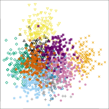
(a) Assumptions met

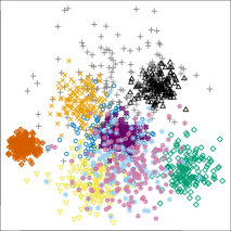
(b) Varying cluster scale

(c) Varying cluster shape

Figure 3: Plots of typical simulated data sets from Gaussian mixtures with 10 clusters in 10 dimensions. Plots show data projected onto their first two principal components. Clusters are differentiated by colour and by point character

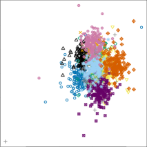
(a) Long tails ($t_{3}$)

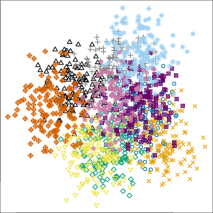
(b) Uniform clusters

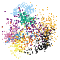
(c) Non-convex clusters

Figure 4: Plots of typical simulated data sets from non-Gaussian mixtures with 10 clusters in 10 dimensions. Plots show data projected onto their first two principal components. Clusters are differentiated by colour and by point character

The results from the simulations are summarised in Tables 1 and 2. For each simulation scheme 30 data sets were generated, and the best performing methods, in terms of quality of solutions selected (see below), are indicated by bold font. In addition, methods whose performance was not significantly different from the best, based on a paired Wilcoxon signed rank test using a $p$-value threshold of 0.01, are also highlighted. We chose to use a small $p$-value to retain considerable discrimination in the results among the methods which perform well in general, but not so small that a single or few instances of one method identifying a single extra cluster would lead to it being excluded from the “best performers” for a given simulation scenario. Methods are compared based on their ability to select the correct number of clusters, and also based on the quality of the clustering solutions selected when compared to the ground truth. For this we use the adjusted Rand index (Hubert and Arabie, 1985, ARI). The Rand index (Rand, 1971) is given as the proportion of pairs of points which are either grouped together in both the clustering solution and the ground truth or assigned to different clusters both in the solution and the ground truth. An adjustment is then applied to normalise this proportion based on its expectation under a random assignment. The clustering accuracy is important to consider since it provides a means for comparing solutions when incorrect values of $k$ are selected. Table 1 shows the results corresponding to data sets generated from Gaussian mixtures. Both the proposed approach, described as BIC${}_{\widehat{edf}}$, and the Silhouette Index show very strong performance. The Jump Statistic performs very well when the assumptions are met exactly, but the performance drops dramatically when these assumptions are deviated from. It is worth noting that of the methods compared, the Silhouette Index is the only approach which is incapable of discerning “one cluster” from “more than one cluster”. It is possible, therefore, that the performance of this method is in some sense slightly over-estimated, since its fail-cases are not as severe.

Table 2 shows the results corresponding to data sets generated from non-Gaussian mixtures. In this case the Silhouette Index enjoys the best performance. The performance of the proposed method is also strong, but significantly below that of the Silhouette in a number of cases, most frequently on the data containing non-convex clusters. The Gap Statistic here showed numerous instances of a failure to identify the presence of clusters. This is an interesting point to note, as in our experiments on data from real applications, the Gap Statistic performs well in general on non-Gaussian data.

Table 1: Results from simulated Gaussian mixture data sets. The Median of the number of clusters selected by each method ($\hat{k}$) and corresponding adjusted Rand index (ARI) are reported. Subscripts show the 10^th and 90^th centiles. The quantiles are based on the results from 30 data sets generated for each simulation set-up. Highest performances for each scenario are highlighted , as are those which are not significantly different from the highest based on a paired Wilcoxon signed rank test with $p$-value threshold of 0.01.

			fK		Gap		Silh.		Jump		BIC		BIC${}_{\widehat{edf}}$
Simulation	k	d	$\hat{k}$	ARI	$\hat{k}$	ARI	$\hat{k}$	ARI	$\hat{k}$	ARI	$\hat{k}$	ARI	$\hat{k}$	ARI
Assump-	5	5	$5_{3,5}$	$98_{59,99}$	$5_{5,5}$	${\bf 98_{97,99}}$	$5_{5,5}$	${\bf 98_{97,99}}$	$5_{5,5}$	${\bf 98_{97,99}}$	$24_{18,29}$	$30_{25,38}$	$5_{5,5}$	${\bf 98_{98,99}}$
tions		10	$4_{2,5}$	$74_{31,96}$	$5_{5,5}$	${\bf 94_{92,97}}$	$5_{5,5}$	${\bf 94_{92,97}}$	$5_{5,5}$	${\bf 94_{92,97}}$	$19_{15,21}$	$35_{32,43}$	$5_{5,5}$	${\bf 94_{92,97}}$
met		15	$2_{2,4}$	$29_{20,70}$	$5_{1,5}$	${\bf 85_{0,87}}$	$5_{5,5}$	${\bf 86_{83,87}}$	$5_{5,29}$	${\bf 86_{21,87}}$	$12_{9,14}$	$45_{39,58}$	$5_{1,5}$	$84_{0,87}$
	10	5	$8_{2,10}$	$79_{17,97}$	$10_{1,10}$	$94_{0,98}$	$10_{10,10}$	${\bf 96_{94,98}}$	$10_{10,10}$	${\bf 96_{94,98}}$	$20_{17,26}$	$66_{56,74}$	$10_{10,11}$	${\bf 96_{92,98}}$
		10	$7_{2,10}$	$62_{14,94}$	$6_{1,10}$	$44_{0,93}$	$10_{10,10}$	${\bf 92_{90,94}}$	$10_{10,10}$	${\bf 92_{90,94}}$	$16_{14,17}$	$73_{68,81}$	$10_{10,10}$	${\bf 92_{89,94}}$
		15	$2_{2,2}$	$12_{11,14}$	$1_{1,10}$	$0_{0,81}$	$10_{10,10}$	${\bf 82_{80,85}}$	$10_{10,10}$	${\bf 82_{80,85}}$	$11_{10,12}$	$78_{74,82}$	$10_{10,10}$	${\bf 82_{80,85}}$
	15	5	$12_{2,14}$	$78_{12,90}$	$2_{1,15}$	$12_{0,95}$	$15_{14,15}$	${\bf 93_{88,96}}$	$15_{14,15}$	${\bf 93_{88,96}}$	$24_{20,29}$	$75_{66,84}$	$15_{15,16}$	${\bf 94_{89,96}}$
		10	$11_{2,15}$	$66_{9,91}$	$1_{1,15}$	$0_{0,91}$	$15_{15,15}$	${\bf 90_{85,92}}$	$15_{15,15}$	${\bf 90_{86,92}}$	$17_{16,18}$	$86_{82,88}$	$15_{15,16}$	${\bf 89_{86,92}}$
		15	$2_{2,12}$	$8_{7,63}$	$1_{1,1}$	$0_{0,0}$	$15_{15,15}$	${\bf 79_{76,81}}$	$15_{15,15}$	${\bf 79_{75,81}}$	$15_{15,15}$	${\bf 79_{76,81}}$	$16_{15,16}$	$78_{75,80}$
Within	5	5	$5_{2,5}$	${\bf 94_{38,99}}$	$5_{5,6}$	$94_{78,99}$	$5_{5,5}$	${\bf 96_{88,99}}$	$5_{5,29}$	$94_{35,99}$	$13_{8,19}$	$69_{50,82}$	$5_{5,5}$	${\bf 96_{90,99}}$
cluster		10	$4_{2,5}$	$73_{27,97}$	$5_{5,6}$	${\bf 91_{83,97}}$	$7_{5,13}$	$87_{75,97}$	$26_{5,29}$	$59_{39,97}$	$17_{11,23}$	$64_{52,75}$	$5_{5,6}$	${\bf 91_{85,97}}$
scale		15	$2_{2,5}$	$31_{20,82}$	$5_{5,6}$	${\bf 84_{78,93}}$	$14_{5,28}$	$73_{59,94}$	$28_{5,30}$	$54_{45,94}$	$14_{11,17}$	$64_{58,76}$	$5_{5,6}$	${\bf 84_{78,94}}$
varies	10	5	$9_{5,10}$	$80_{45,95}$	$10_{1,10}$	$91_{0,98}$	$10_{10,14}$	${\bf 93_{86,98}}$	$10_{10,24}$	${\bf 93_{71,98}}$	$19_{15,25}$	$79_{71,86}$	$11_{10,12}$	$91_{82,96}$
		10	$7_{2,10}$	$62_{14,92}$	$10_{1,11}$	${\bf 85_{0,92}}$	$14_{10,24}$	$85_{76,93}$	$10_{10,29}$	${\bf 86_{68,93}}$	$19_{13,22}$	$78_{71,85}$	$11_{10,12}$	${\bf 86_{81,93}}$
		15	$2_{2,8}$	$14_{11,71}$	$10_{1,10}$	$76_{0,85}$	$23_{13,30}$	$73_{66,82}$	$28_{10,30}$	$69_{62,89}$	$13_{10,15}$	$77_{70,81}$	$11_{10,16}$	${\bf 80_{72,89}}$
	15	5	$13_{11,15}$	$80_{70,88}$	$4_{1,15}$	$26_{0,90}$	$15_{15,17}$	${\bf 89_{85,95}}$	$15_{14,18}$	$89_{84,95}$	$15_{14,15}$	$85_{76,91}$	$16_{15,19}$	$88_{81,94}$
		10	$11_{2,14}$	$66_{10,86}$	$1_{1,15}$	$0_{0,89}$	$19_{15,24}$	${\bf 85_{79,91}}$	$15_{14,16}$	${\bf 87_{77,91}}$	$20_{16,23}$	$83_{77,88}$	$17_{15,19}$	${\bf 86_{78,90}}$
		15	$7_{2,14}$	$42_{8,72}$	$11_{1,15}$	$0_{0,82}$	$29_{26,30}$	$74_{69,78}$	$26_{15,29}$	${\bf 75_{72,82}}$	$19_{16,22}$	${\bf 77_{72,81}}$	$16_{9,21}$	${\bf 77_{51,82}}$
Within	5	5	$5_{3,5}$	${\bf 98_{60,100}}$	$5_{5,6}$	${\bf 98_{87,99}}$	$5_{5,5}$	${\bf 98_{95,100}}$	$24_{5,30}$	$34_{26,98}$	$15_{10,25}$	$48_{31,68}$	$5_{5,5}$	${\bf 98_{94,100}}$
cluster		10	$4_{2,5}$	$76_{33,97}$	$5_{5,8}$	${\bf 94_{74,98}}$	$5_{5,5}$	${\bf 95_{92,98}}$	$28_{24,30}$	$27_{25,33}$	$20_{14,25}$	$38_{29,48}$	$5_{5,5}$	${\bf 95_{90,98}}$
shape		15	$2_{2,5}$	$30_{21,88}$	$5_{5,5}$	${\bf 86_{83,92}}$	$5_{5,5}$	${\bf 87_{83,92}}$	$29_{26,30}$	$24_{22,28}$	$18_{15,22}$	$34_{29,43}$	$5_{5,5}$	${\bf 86_{81,92}}$
varies	10	5	$9_{7,10}$	$85_{67,97}$	$10_{1,10}$	$94_{0,97}$	$10_{10,10}$	${\bf 95_{92,97}}$	$27_{10,30}$	$55_{50,94}$	$22_{17,25}$	$65_{56,79}$	$10_{10,11}$	$94_{90,96}$
		10	$7_{2,10}$	$67_{13,94}$	$10_{1,10}$	$90_{0,94}$	$10_{10,10}$	${\bf 92_{88,95}}$	$28_{21,30}$	$51_{46,63}$	$21_{17,25}$	$63_{52,72}$	$11_{10,11}$	$91_{86,93}$
		15	$2_{2,8}$	$13_{11,70}$	$6_{1,10}$	$46_{0,87}$	$10_{10,11}$	${\bf 84_{80,88}}$	$28_{25,30}$	$46_{42,51}$	$19_{15,25}$	$61_{52,72}$	$11_{10,11}$	${\bf 83_{81,87}}$
	15	5	$14_{10,15}$	$83_{63,90}$	$6_{1,15}$	$41_{0,95}$	$15_{14,15}$	${\bf 91_{86,96}}$	$15_{14,29}$	$90_{70,95}$	$22_{16,26}$	$80_{72,88}$	$16_{15,18}$	${\bf 90_{85,95}}$
		10	$11_{2,14}$	$67_{9,84}$	$1_{1,15}$	$0_{0,91}$	$15_{15,15}$	${\bf 91_{86,94}}$	$15_{15,30}$	$87_{64,94}$	$23_{18,26}$	$76_{69,85}$	$16_{15,17}$	$88_{85,92}$
		15	$2_{2,12}$	$8_{6,66}$	$1_{1,15}$	$0_{0,80}$	$15_{15,16}$	${\bf 82_{78,86}}$	$28_{25,29}$	$62_{57,65}$	$20_{17,23}$	$72_{66,79}$	$16_{15,17}$	$80_{76,85}$

Table 2: Results from simulated non-Gaussian mixture data sets. The Median of the number of clusters selected by each method ($\hat{k}$) and corresponding adjusted Rand index (ARI) are reported. Subscripts show the 10^th and 90^th centiles. The quantiles are based on the results from 30 data sets generated for each simulation set-up. Highest performances for each scenario are highlighted , as are those which are not significantly different from the highest based on a paired Wilcoxon signed rank test with $p$-value threshold of 0.01.

			fK		Gap		Silh.		Jump		BIC		BIC${}_{\widehat{edf}}$
Simulation	k	d	$\hat{k}$	ARI	$\hat{k}$	ARI	$\hat{k}$	ARI	$\hat{k}$	ARI	$\hat{k}$	ARI	$\hat{k}$	ARI
Long	5	5	$5_{2,5}$	$92_{36,95}$	$5_{1,5}$	$92_{0,94}$	$6_{5,6}$	${\bf 93_{90,95}}$	$5_{5,6}$	${\bf 93_{90,95}}$	$21_{14,26}$	$41_{34,58}$	$5_{5,6}$	${\bf 93_{90,95}}$
tails ($t_{3}$)		10	$3_{2,5}$	$52_{29,86}$	$1_{1,5}$	$0_{0,90}$	$6_{5,8}$	$86_{83,90}$	$27_{5,30}$	$36_{32,87}$	$9_{7,14}$	$77_{62,85}$	$5_{5,7}$	${\bf 87_{84,90}}$
		15	$2_{2,4}$	$26_{19,64}$	$1_{1,1}$	$0_{0,8}$	$6_{2,7}$	${\bf 78_{23,81}}$	$28_{24,30}$	$34_{30,39}$	$13_{9,18}$	$61_{43,69}$	$5_{1,22}$	$59_{0,81}$
	10	5	$8_{2,10}$	$72_{17,90}$	$1_{1,10}$	$0_{0,90}$	$11_{10,12}$	${\bf 90_{86,92}}$	$10_{10,12}$	${\bf 89_{78,92}}$	$18_{12,23}$	$77_{70,89}$	$11_{10,12}$	${\bf 90_{87,92}}$
		10	$3_{2,9}$	$15_{13,74}$	$1_{1,2}$	$0_{0,8}$	$13_{11,14}$	${\bf 82_{80,86}}$	$24_{10,30}$	$68_{60,85}$	$12_{11,14}$	${\bf 83_{79,86}}$	$11_{11,13}$	${\bf 82_{80,86}}$
		15	$2_{2,10}$	$12_{10,70}$	$1_{1,1}$	$0_{0,0}$	$15_{11,17}$	${\bf 72_{67,75}}$	$28_{24,30}$	$59_{53,66}$	$15_{12,17}$	${\bf 71_{67,75}}$	$11_{10,13}$	${\bf 73_{68,75}}$
	15	5	$11_{2,14}$	$64_{11,82}$	$1_{1,14}$	$0_{0,83}$	$16_{14,18}$	${\bf 85_{81,89}}$	$15_{14,17}$	${\bf 85_{78,89}}$	$19_{16,26}$	$81_{77,88}$	$16_{13,18}$	${\bf 85_{77,88}}$
		10	$11_{2,15}$	$60_{9,78}$	$1_{1,1}$	$0_{0,0}$	$19_{16,22}$	${\bf 80_{76,83}}$	$23_{16,28}$	${\bf 78_{72,83}}$	$18_{16,22}$	${\bf 80_{75,84}}$	$17_{10,18}$	${\bf 80_{48,83}}$
		15	$13_{2,17}$	$56_{7,65}$	$1_{1,1}$	$0_{0,0}$	$23_{19,25}$	${\bf 68_{66,74}}$	$28_{23,30}$	$66_{62,70}$	$19_{16,22}$	${\bf 69_{65,74}}$	$18_{15,20}$	${\bf 69_{63,72}}$
Uniform	5	5	$5_{2,5}$	$100_{38,100}$	$5_{5,5}$	${\bf 100_{98,100}}$	$5_{5,5}$	${\bf 100_{98,100}}$	$5_{5,5}$	${\bf 100_{99,100}}$	$25_{17,30}$	$30_{25,39}$	$5_{5,5}$	${\bf 100_{99,100}}$
clusters		10	$4_{2,5}$	$76_{32,97}$	$5_{1,5}$	${\bf 96_{0,98}}$	$5_{5,5}$	${\bf 96_{94,98}}$	$5_{5,5}$	${\bf 96_{95,98}}$	$18_{15,22}$	$38_{31,45}$	$5_{5,5}$	${\bf 96_{95,98}}$
		15	$2_{2,5}$	$28_{20,84}$	$5_{1,5}$	${\bf 86_{0,88}}$	$5_{5,5}$	${\bf 86_{84,88}}$	$5_{5,29}$	${\bf 86_{20,88}}$	$13_{11,14}$	$43_{39,48}$	$5_{1,5}$	$85_{0,88}$
	10	5	$8_{2,10}$	$80_{17,99}$	$10_{1,10}$	$95_{0,99}$	$10_{10,10}$	${\bf 99_{96,100}}$	$10_{10,10}$	${\bf 99_{97,100}}$	$21_{17,27}$	$65_{53,75}$	$10_{10,11}$	$97_{92,99}$
		10	$2_{2,10}$	$16_{13,95}$	$1_{1,10}$	$0_{0,95}$	$10_{10,10}$	${\bf 94_{91,96}}$	$10_{10,10}$	${\bf 94_{91,96}}$	$17_{14,19}$	$71_{65,79}$	$10_{10,11}$	${\bf 93_{91,96}}$
		15	$2_{2,2}$	$12_{10,13}$	$1_{1,2}$	$0_{0,8}$	$10_{10,10}$	${\bf 84_{81,86}}$	$10_{10,10}$	${\bf 83_{80,85}}$	$11_{11,13}$	$79_{72,84}$	$10_{10,10}$	${\bf 83_{79,85}}$
	15	5	$12_{2,14}$	$80_{13,92}$	$14_{1,15}$	$89_{0,98}$	$15_{14,15}$	$97_{89,98}$	$15_{14,15}$	${\bf 96_{90,98}}$	$23_{20,29}$	$82_{68,86}$	$15_{15,16}$	${\bf 95_{91,98}}$
		10	$8_{2,14}$	$48_{9,89}$	$1_{1,15}$	$0_{0,93}$	$15_{15,15}$	${\bf 93_{90,95}}$	$15_{14,15}$	${\bf 93_{89,94}}$	$17_{16,17}$	$90_{86,92}$	$16_{15,16}$	${\bf 92_{88,94}}$
		15	$2_{2,13}$	$8_{7,71}$	$1_{1,1}$	$0_{0,0}$	$15_{15,15}$	${\bf 81_{78,84}}$	$15_{14,15}$	${\bf 81_{75,84}}$	$15_{15,15}$	${\bf 81_{78,85}}$	$15_{15,16}$	$80_{76,84}$
Non-	5	5	$5_{4,5}$	${\bf 82_{68,91}}$	$9_{1,11}$	$68_{0,81}$	$6_{5,8}$	${\bf 81_{71,89}}$	$26_{22,30}$	$31_{28,44}$	$22_{16,25}$	$37_{31,56}$	$8_{6,11}$	$76_{66,85}$
convex		10	$4_{2,5}$	$50_{24,86}$	$14_{11,18}$	$49_{34,59}$	$9_{6,12}$	${\bf 68_{53,86}}$	$28_{26,30}$	$27_{24,30}$	$22_{17,30}$	$31_{24,45}$	$9_{5,12}$	${\bf 62_{42,81}}$
clusters		15	$2_{2,4}$	$31_{23,60}$	$15_{1,18}$	$42_{0,55}$	$12_{6,16}$	${\bf 50_{38,85}}$	$29_{28,30}$	$25_{23,28}$	$23_{16,29}$	$30_{24,43}$	$9_{4,16}$	${\bf 57_{43,81}}$
	10	5	$10_{9,10}$	${\bf 90_{85,95}}$	$10_{1,11}$	$89_{0,95}$	$10_{10,11}$	${\bf 92_{85,95}}$	$10_{10,28}$	$85_{57,95}$	$19_{15,23}$	$74_{63,83}$	$12_{11,14}$	$88_{82,93}$
		10	$9_{8,10}$	$83_{69,95}$	$13_{1,16}$	$79_{0,87}$	$10_{10,14}$	${\bf 91_{81,96}}$	$28_{26,30}$	$57_{51,60}$	$22_{16,30}$	$65_{51,81}$	$14_{12,21}$	$85_{66,91}$
		15	$9_{8,10}$	$82_{65,91}$	$16_{10,19}$	$74_{49,85}$	$12_{10,13}$	${\bf 88_{78,96}}$	$29_{26,30}$	$51_{48,56}$	$22_{17,27}$	$61_{52,72}$	$13_{11,17}$	$81_{64,91}$
	15	5	$14_{12,15}$	$88_{79,94}$	$15_{1,16}$	$90_{0,96}$	$15_{15,16}$	${\bf 93_{90,97}}$	$16_{15,27}$	$92_{71,97}$	$20_{16,25}$	$85_{76,92}$	$17_{16,19}$	$91_{84,94}$
		10	$14_{13,15}$	$93_{84,98}$	$15_{12,18}$	$94_{74,99}$	$15_{15,17}$	${\bf 97_{91,99}}$	$28_{26,30}$	$76_{70,80}$	$20_{15,26}$	$89_{75,95}$	$18_{15,21}$	$92_{86,97}$
		15	$15_{12,15}$	$92_{79,99}$	$16_{1,17}$	$94_{0,97}$	$15_{15,16}$	${\bf 98_{95,99}}$	$28_{27,30}$	$73_{70,79}$	$23_{17,26}$	$83_{74,95}$	$17_{16,19}$	$94_{88,97}$

4.2 Public Benchmark Data

This section presents briefly on results from experiments using a large collection of 28 publicly available data sets associated with real applications from diverse fields. These are popular benchmark data sets taken from the UCI machine learning repository (Bache and Lichman, 2013), with the exception of the Yeast and Phoneme data sets. These data sets were chosen since ground-truth label sets are available, which can be used for validation and comparison of clustering solutions. All data sets were standardised to have unit variance in every dimension before applying any clustering.

Table 3 shows the results of these experiments. The numbers in brackets indicate the true number of clusters, $k$. For each method the selected number of clusters, $\hat{k}$, and the adjusted Rand index are reported. For each data set we have also included the “Ideal” $k$-means solution, which corresponds with the solution that attains the highest ARI value. We find this to be pertinent since when the data distribution deviates substantially from the $k$-means assumptions it may be that the best $k$-means solution does not contain the same number of clusters as the ground truth. Furthermore, although it is unlikely that there exists a method which will reliably select the ideal solution, it is also very likely that there exists, theoretically, a method which performs better than any of the methods considered herein. Comparing with the ideal performance therefore gives a bound on how much better it is possible to perform with any model selection technique for $k$-means. The ideal performance also gives us some indication of the difficulty of the clustering problem. Two immediate take-aways from the table are that the fK method selected two clusters in almost all cases, while the Jump Statistic dramatically over-estimated the number of clusters in all but a few instances. The BIC with naïve setting of the degrees of freedom also over-esimates the number of clusters considerably in general, but not by so large a margin as the Jump Statistic. The Silhouette Index, Gap Statistic and the BIC with the effective degrees of freedom all perform quite consistently well. To better illustrate the overall performance of the methods on these data sets, the results of Table 3 are summarised in Figure 5. The figure shows boxplots of the ARI performance regret, when compared to the ideal performance, normalised for difficulty. That is, for a method $M$ and data set $\mathbf{X}$, the normalised regret is given by

$$\frac{\mbox{ARI(Ideal(}\mathbf{X}))-\mbox{ARI(}M(\mathbf{X}))}{\mbox{ARI(Ideal(}\mathbf{X}))}.$$

The figure also shows the mean of the normalised regret for each method, indicated by a red dot. Here we see that the Gap Statistic and the BIC using the proposed estimate of effective degrees of freedom perform substantially better than the other methods, in general. While the Silhouette Index yields a similar median performance, its instances of poor performance are considerably worse than those of the Gap and proposed BIC variant.

Given the variety and number of the data sets used in these experiments, there is strong evidence that the proposed estimation procedure for the effective degrees of freedom leads to selection of models which enjoy very strong performance when compared with existing techniques.

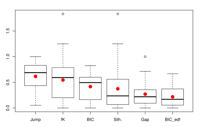
Figure 5: Boxplots of normalised regret (when compared with the ideal performance). Mean normalised regret is indicated in each case by a red dot.

Table 3: Results from publicly available benchmark data sets. Number of clusters selected by each method ($\hat{k}$) and corresponding adjusted Rand index (ARI) are reported.

	fK		Gap		Silh.		Jump		BIC		BIC${}_{\widehat{edf}}$		Ideal
Data set $(k)$	$\hat{k}$	ARI	$\hat{k}$	ARI	$\hat{k}$	ARI	$\hat{k}$	ARI	$\hat{k}$	ARI	$\hat{k}$	ARI	$\hat{k}$	ARI
Wine (3)	2	0.37	3	0.9	3	0.9	30	0.13	11	0.35	3	0.9	3	0.9
Seeds (3)	2	0.48	3	0.77	2	0.48	29	0.12	17	0.2	3	0.77	3	0.77
Ionosphere (2)	2	0.17	8	0.17	4	0.28	30	0.11	12	0.12	4	0.28	3	0.29
Votes (2)	2	0.57	7	0.21	2	0.57	29	0.06	14	0.1	4	0.32	2	0.57
Iris (3)	2	0.57	3	0.62	2	0.57	27	0.14	14	0.3	3	0.62	3	0.62
Libras (15)	2	0.07	13	0.31	18	0.31	29	0.29	16	0.32	16	0.32	20	0.34
Heart (2)	2	0.34	2	0.34	5	0.29	29	0.04	5	0.29	5	0.29	2	0.34
Glass (6)	2	0.19	9	0.17	2	0.19	29	0.13	13	0.24	4	0.2	5	0.24
Mammography (2)	2	0.39	3	0.31	3	0.31	25	0.05	11	0.13	4	0.31	2	0.39
Parkinsons (2)	2	-0.1	7	0.07	2	-0.1	30	0.03	12	0.05	10	0.04	6	0.12
Yeast (5)	2	0.42	8	0.4	2	0.42	29	0.14	10	0.39	12	0.36	4	0.57
Forest (4)	2	0.18	5	0.39	2	0.18	30	0.15	19	0.2	12	0.28	4	0.45
Breast Cancer (2)	2	0.82	9	0.38	2	0.82	30	0.15	17	0.34	4	0.76	2	0.82
Dermatology (6)	2	0.21	6	0.7	3	0.57	28	0.26	9	0.65	6	0.7	5	0.84
Synth (6)	2	0.27	8	0.67	2	0.27	30	0.35	10	0.65	10	0.65	8	0.67
Soy Bean (19)	2	0.05	16	0.43	2	0.05	30	0.42	16	0.43	16	0.43	18	0.56
Olive Oil (3/9)	2	0.4	10	0.49	5	0.67	30	0.19	18	0.17	9	0.5	5	0.67
Bank (2)	2	0.01	3	0.06	18	0.1	26	0.09	24	0.09	21	0.1	5	0.21
Optidigits (10)	2	0.13	17	0.57	20	0.6	30	0.47	18	0.65	18	0.65	18	0.65
Image Seg (7)	2	0.17	14	0.46	6	0.48	28	0.3	14	0.46	14	0.46	9	0.51
MF Digits (10)	2	0.15	18	0.62	9	0.65	1	0	20	0.59	20	0.59	11	0.68
Satellite (6)	3	0.29	12	0.41	3	0.29	30	0.25	16	0.35	16	0.35	7	0.56
Texture (11)	2	0.11	23	0.41	2	0.11	30	0.41	30	0.41	30	0.41	11	0.5
Pen Digits (10)	2	0.13	30	0.45	8	0.45	28	0.46	30	0.45	21	0.53	14	0.64
Phoneme (5)	2	0.16	11	0.45	2	0.16	1	0	21	0.28	21	0.28	5	0.64
Frogs (4/8/10)	2	0.46	17	0.21	3	0.5	25	0.14	17	0.15	15	0.24	4	0.57
Auto (3)	2	-0.04	4	0.13	2	-0.04	26	0.05	24	0.03	4	0.13	5	0.16
Yeast UCI (10)	7	0.19	1	0	6	0.11	9	0.18	4	0.1	9	0.18	7	0.19

5 Discussion

This work investigated the effective degrees of freedom in the $k$-means model. We argued that the degrees of freedom estimate based on the number of explicitly estimated parameters is an inappropriate pairing with the so-called classification likelihood for performing model selection for $k$-means. This is because the classification likelihood assumes the clustering assignment forms part of the estimation, but this added estimation is not accounted for in the model dimension. The proposed formulation accommodates the uncertainty of the class assignments in the degrees of freedom, where an extension of Stein’s lemma showed that these uncertainties are appropriately accommodated by considering the size and location of the discontinuities in the $k$-means model, which correspond precisely to the reassignments of points to different clusters. Evaluating the new degrees of freedom expression is challenging, however a few simplifications allowed us to approximate this value in practice. The approximation was validated through model selection within the Bayesian Information Criterion. Experiments using simulated data, as well as a large collection of publicly available benchmark data sets suggest that this approach is competitive with popular existing methods for model selection in $k$-means clustering.

Proofs

Proof of Lemma 1

Let $X\sim N(\mu,\sigma^{2})$ and consider any $g:\mathbb{R}\to\mathbb{R}$ which is Lipschitz on $(-\infty,\delta)$ and $(\delta,\infty)$ for some $\delta\in\mathbb{R}$. For each $\epsilon>0$ define

$$g_{\epsilon}(x)=\left\{\begin{array}[]{ll}g(x),&x\not\in\mathcal{B}_{\epsilon}(\delta)\\ g(\delta-\epsilon)+[g(\delta+\epsilon)-g(\delta-\epsilon)]\frac{x-(\delta-\epsilon)}{2\epsilon},&x\in\mathcal{B}_{\epsilon}(\delta),\end{array}\right.$$

where $\mathcal{B}_{\epsilon}(\delta)=(\delta-\epsilon,\delta+\epsilon)$. Then $g_{\epsilon}$ is Lipschitz by construction and so by (Candes et al., 2013, Lemma 3.2) we know $g_{\epsilon}$ is almost differentiable and $E[g_{\epsilon}^{\prime}(X)^{2}]<\infty$, and so by (Stein, 1981, Lemma 2) we have

$$\frac{1}{\sigma^{2}}E[(X-\mu)g_{\epsilon}(X)]=E[g^{\prime}_{\epsilon}(X)].$$

But

$$E[g^{\prime}_{\epsilon}(X)]= E\left[g_{\epsilon}^{\prime}(X)|X\not\in\mathcal{B}_{\epsilon}(\delta)\right]P(X\not\in\mathcal{B}_{\epsilon}(\delta))+E\left[g_{\epsilon}^{\prime}(X)|X\in\mathcal{B}_{\epsilon}(\delta)\right]P(X\in\mathcal{B}_{\epsilon}(\delta))$$

$$= E\left[g^{\prime}(X)|X\not\in\mathcal{B}_{\epsilon}(\delta)\right]P(X\not\in\mathcal{B}_{\epsilon}(\delta))+\frac{g(\delta+\epsilon)-g(\delta-\epsilon)}{2\epsilon}P(X\in\mathcal{B}_{\epsilon}(\delta)).$$

Taking the limit as $\epsilon\to 0^{+}$ gives

$$\frac{1}{\sigma^{2}}E[(X- \mu)g(X)]=E[g^{\prime}(X)]+\left(\lim_{\gamma\downarrow\delta}g(\gamma)-\lim_{\gamma\uparrow\delta}g(\gamma)\right)\frac{1}{\sqrt{2\pi}\sigma}e^{\frac{-1}{2\sigma^{2}}(\delta-\mu)^{2}},$$

as required. The extension to any $g$ with finitely many such discontinuity points arises from a very simple induction.

We therefore have for any $i,j$, that

$$\frac{1}{\sigma^{2}}E\bigg{[}(\mathbf{X}_{i,j}-{{\upmu}}_{i,j})f (\mathbf{X})_{i,j}\bigg{|}\{\mathbf{X}_{k,l}\}_{(k,l)\not=(i,j)}\bigg{]}=E\left[\frac{\partial}{\partial X_{i,j}}f(\mathbf{X})_{i,j}\bigg{|}\{\mathbf{X}_{k,l}\}_{(k,l)\not=(i,j)}\right]$$

$$+\sum_{\begin{subarray}{c}\delta:\mathbf{X}_{i,j}+\delta\in\\ \mathcal{D}(\{\mathbf{X}_{k,l}\}_{(k,l)\not=(i,j)})\end{subarray}}\frac{1}{\sigma}\phi\left(\frac{\mathbf{X}_{i,j}+\delta-{{\upmu}}_{i,j}}{\sigma}\right)\lim_{\gamma\downarrow\uparrow\delta}f(\mathbf{X}+\gamma\mathbf{e}_{i,j})_{i,j}$$

The result follows from the law of total expectation. $\square$

Proof of Lemma 2

Notice that the discontinuities in $\mathcal{M}(\mathbf{X})_{i,j}$ can occur only when there is a change in the assignment of one of the observations. If this occurs at the point $\mathbf{X}+\delta\mathbf{e}_{i,j}$, then it is straightforward to show that

$$|\lim_{\gamma\downarrow\uparrow\delta}\mathcal{M}(\mathbf{X}+\gamma\mathbf{e}_{i,j})_{i,j}|\leq\mathrm{Diam}(\mathbf{X})+C|\delta|,$$

where Diam$(\mathbf{X})$ is the diameter of the rows of $\mathbf{X}$ and $C$ is a constant independent of $\mathbf{X}$. There are also clearly finitely many such discontinuities since there are finitely many cluster solutions arising from $n$ data, i.e.,

$$|\mathcal{D}(\{\mathbf{X}_{k,l}\}_{(k,l)\not=(i,j)})|\leq A,$$

for some constant $A$ independent of $i,j,\mathbf{X}$. Furthermore $|\mathcal{M}(\mathbf{X}+\gamma\mathbf{e}_{i,j})_{i,j}-\mathcal{M}(\mathbf{X})_{i,j}|\leq\gamma$ as long as all cluster assignments remain the same, and hence $\mathcal{M}(\mathbf{X}+\gamma\mathbf{e}_{i,j})_{i,j}$ is Lipschitz as a function of $\gamma$ between points of discontinuity. Finally,

$$E\Bigg{[}\Bigg{|}\sum_{\begin{subarray}{c}\delta:\mathbf{X}_{i,j}+\delta\in\\ \mathcal{D}(\{\mathbf{X}_{k,l}\}_{(k,l)\not=(i,j)})\end{subarray}}\phi\left(\frac{\mathbf{X}_{i,j}+\delta-{{\upmu}}_{i,j}}{\sigma}\right)\lim_{\gamma\downarrow\uparrow\delta}\mathcal{M}(\mathbf{X}+\gamma\mathbf{e}_{i,j})_{i,j}\Bigg{|}\Bigg{]}$$

$$\leq E\Bigg{[}\sum_{\begin{subarray}{c}\delta:\mathbf{X}_{i,j}+\delta\in\\ \mathcal{D}(\{\mathbf{X}_{k,l}\}_{(k,l)\not=(i,j)})\end{subarray}}\phi\left(\frac{\mathbf{X}_{i,j}+\delta-{{\upmu}}_{i,j}}{\sigma}\right)(\mathrm{Diam}(\mathbf{X})+C|\delta|)\Bigg{]}$$

$$\leq\frac{A}{\sqrt{2\pi}}\bigg{(}E[\mathrm{Diam}(\mathbf{X})]+CE\left[|\mathbf{X}_{i,j}-{{\upmu}}_{i,j}|+(\mathbf{X}_{i,j}-{{\upmu}}_{i,j})^{2}+4\sigma^{2}\right]\bigg{)},$$

since $\phi((a-\delta)/\sigma)|\delta|$ is maximised by a $\delta$ satisfying $|\delta|\leq(|a|+|a^{2}-4\sigma^{2}|)/2$, and $\phi$ is bounded above by $1/\sqrt{2\pi}$. Now, the tail of the distribution of $\mathrm{Diam}(\mathbf{X})$ is similar to that of the distribution of the maximum of $n$ $\chi$ random variables with $d$ degrees of freedom. Therefore $E[\mbox{Diam}(\mathbf{X})]$ is clearly finite. The second term above is clearly finite, since $\mathbf{X}_{i,j}-{{\upmu}}_{i,j}$ is normally distributed, and hence the expectation in Lemma 2 exists and is finite. $\square$

References

- Akaike [1998] Hirotogu Akaike. Information theory and an extension of the maximum likelihood principle. In Selected papers of Hirotugu Akaike, pages 199–213. Springer, 1998.
- Bache and Lichman [2013] K. Bache and M. Lichman. UCI machine learning repository, 2013. URL http://archive.ics.uci.edu/ml.
- Candes et al. [2013] Emmanuel J Candes, Carlos A Sing-Long, and Joshua D Trzasko. Unbiased risk estimates for singular value thresholding and spectral estimators. IEEE transactions on signal processing, 61(19):4643–4657, 2013.
- Celeux and Govaert [1992] Gilles Celeux and Gérard Govaert. A classification em algorithm for clustering and two stochastic versions. Computational statistics & Data analysis, 14(3):315–332, 1992.
- Efron [1986] Bradley Efron. How biased is the apparent error rate of a prediction rule? Journal of the American statistical Association, 81(394):461–470, 1986.
- Fraley and Raftery [2002] Chris Fraley and Adrian E Raftery. Model-based clustering, discriminant analysis, and density estimation. Journal of the American statistical Association, 97(458):611–631, 2002.
- Hamerly and Elkan [2004] Greg Hamerly and Charles Elkan. Learning the k in k-means. In Advances in neural information processing systems, pages 281–288, 2004.
- Hofmeyr [2019] David P Hofmeyr. Improving spectral clustering using the asymptotic value of the normalized cut. Journal of Computational and Graphical Statistics, pages 1–13, 2019.
- Hubert and Arabie [1985] Lawrence Hubert and Phipps Arabie. Comparing partitions. Journal of classification, 2(1):193–218, 1985.
- Jiang et al. [2012] Ke Jiang, Brian Kulis, and Michael I Jordan. Small-variance asymptotics for exponential family dirichlet process mixture models. In Advances in Neural Information Processing Systems, pages 3158–3166, 2012.
- Kaufman and Rousseeuw [2009] Leonard Kaufman and Peter J Rousseeuw. Finding groups in data: an introduction to cluster analysis, volume 344. John Wiley & Sons, 2009.
- Manning et al. [2008] Christopher Manning, Prabhakar Raghavan, and Hinrich Schütze. Introduction to Information Retrieval. Cambridge University Press, 1 edition, 2008.
- Pelleg et al. [2000] Dan Pelleg, Andrew W Moore, et al. X-means: Extending k-means with efficient estimation of the number of clusters. In Icml, volume 1, pages 727–734, 2000.
- Pham et al. [2005] Duc Truong Pham, Stefan S Dimov, and Cuong Du Nguyen. Selection of k in k-means clustering. Proceedings of the Institution of Mechanical Engineers, Part C: Journal of Mechanical Engineering Science, 219(1):103–119, 2005.
- R Core Team [2013] R Core Team. R: A Language and Environment for Statistical Computing. R Foundation for Statistical Computing, Vienna, Austria, 2013. URL http://www.R-project.org/.
- Ramsey et al. [2008] Stephen A Ramsey, Sandy L Klemm, Daniel E Zak, Kathleen A Kennedy, Vesteinn Thorsson, Bin Li, Mark Gilchrist, Elizabeth S Gold, Carrie D Johnson, Vladimir Litvak, et al. Uncovering a macrophage transcriptional program by integrating evidence from motif scanning and expression dynamics. PLoS computational biology, 4(3):e1000021, 2008.
- Rand [1971] William M Rand. Objective criteria for the evaluation of clustering methods. Journal of the American Statistical association, 66(336):846–850, 1971.
- Schwarz et al. [1978] Gideon Schwarz et al. Estimating the dimension of a model. The annals of statistics, 6(2):461–464, 1978.
- Stein [1981] Charles M Stein. Estimation of the mean of a multivariate normal distribution. The annals of Statistics, pages 1135–1151, 1981.
- Sugar and James [2003] Catherine A Sugar and Gareth M James. Finding the number of clusters in a dataset: An information-theoretic approach. Journal of the American Statistical Association, 98(463):750–763, 2003.
- Tibshirani et al. [2001] Robert Tibshirani, Guenther Walther, and Trevor Hastie. Estimating the number of clusters in a data set via the gap statistic. Journal of the Royal Statistical Society: Series B (Statistical Methodology), 63(2):411–423, 2001.
- Tibshirani [2015] Ryan J Tibshirani. Degrees of freedom and model search. Statistica Sinica, pages 1265–1296, 2015.