Mercury’s Internal Structure

Abstract

We describe the current state of knowledge about Mercury’s interior structure. We review the available observational constraints, including mass, size, density, gravity field, spin state, composition, and tidal response. These data enable the construction of models that represent the distribution of mass inside Mercury. In particular, we infer radial profiles of the pressure, density, and gravity in the core, mantle, and crust. We also examine Mercury’s rotational dynamics and the influence of an inner core on the spin state and the determination of the moment of inertia. Finally, we discuss the wide-ranging implications of Mercury’s internal structure on its thermal evolution, surface geology, capture in a unique spin-orbit resonance, and magnetic field generation.

1 Introduction

1.1 Importance of planetary interiors

We seek to understand the interior structures of planetary bodies because the interiors affect planetary properties and processes in several fundamental ways. First, a knowledge of the interior informs us about a planet’s makeup and enables us to test hypotheses related to planet formation. Second, interior properties dictate the thermal evolution of planetary bodies and, consequently, the history of volcanism and tectonics on these bodies. Many geological features are the surface expression of processes that take place below the surface. Third, the structure of the interior and the nature of the interactions among inner core, outer core, and mantle have a profound influence on the evolution of the spin state and the response of the planet to external forces and torques. These processes dictate the planet’s tectonic and insolation regimes and also affect its overall shape. Finally, interior properties control the generation of planetary magnetic fields, and, therefore, the development of magnetospheres.

Four of the six primary science objectives of the MESSENGER mission (Solomon et al.,, 2001) rely on an understanding of the planet’s interior structure. These four mission objectives pertain to the high density of Mercury, its geologic history, the nature of its magnetic field, and the structure of its core.

1.2 Objectives

An ideal representation of a planetary interior would include the description of physical and chemical quantities at every location within the volume of the planetary body at every point in time. Here, we focus on a description of Mercury’s interior at the current epoch. For a description of the evolution of the state of the planet over geologic time, see Chapter 19. Because our ability to specify properties throughout the planetary volume is limited, we simplify the problem by assuming axial or spherical symmetry. Specifically, we seek self-consistent depth profiles of density, pressure, and temperature, informed by observational constraints (radius, mass, moment of inertia, composition). The solution requires the use of equations of state and assumptions about material properties, both guided by laboratory data. We compute the bulk modulus and thermal expansion coefficient as part of the estimation process, and we use the profiles to compute other rheological properties, such as viscosity and additional elastic moduli. Finally, we use our models to numerically evaluate the planet’s tidal response and compare it with observational data. Our models of the interior structure are relevant to a wide range of problems, but Mercury’s unusual insolation and thermal patterns violate our symmetry assumptions. These assumptions must be lifted for certain applications that require precise temperature distributions.

Our primary objective is to provide a family of simplified models of Mercury’s interior that satisfy the currently available observational constraints. A secondary objective is to select, among these models, a recommended model that matches all available constraints. This model may be considered a Preliminary Reference Mercury Model (PRMM), evoking a distant connection with its venerable Earth analog (Dziewonski and Anderson,, 1981).

1.3 Available observational constraints

All of our knowledge about Mercury comes from Earth-based observations, three Mariner 10 flybys, three MESSENGER flybys, and the four-year orbital phase of the MESSENGER mission. In the absence of seismological data, our information about the interior comes primarily from geodesy, the study of the gravity field, shape, and spin state of the planet, including solid-body tides. We will also draw on constraints derived from the surface expression of global contraction and observations of surface composition, with the caveat that the composition at depth may be substantially different from that inferred for surface material. The structure of the magnetic field and its dynamo origin can also be used to inform interior models.

1.4 Outline

The primary observational constraints (Sections 2–4) are used to develop two- and three-layer structural models (Sections 5). We then add compositional constraints (Section 6) and develop multi-layer models (Section 7). We examine the tidal response of the planet (Section 8) and the influence of an inner core (Section 9). We conclude with a discussion of a representative interior model (Section 10) and implications (Section 11).

2 Rotational dynamics

In his classic 1976 paper, Stanton J. Peale described the effects of a molten core on the dynamics of Mercury’s rotation and proposed an ingenious method for measuring the size and state of the core (Peale,, 1976). Most of our knowledge about Mercury’s interior structure can be traced to Peale’s ideas and to the powerful connection between dynamics and geophysics. We review aspects of Mercury’s rotational dynamics that are relevant to determining its interior structure. Peale, (1988) provided a more extensive review.

2.1 Spin-orbit resonance

Radar observations by Pettengill and Dyce, (1965) revealed that the spin period of Mercury differs from its orbital period. To explain the radar results, Colombo, (1965) correctly hypothesized that Mercury rotates on its spin axis three times for every two revolutions around the Sun. Mercury is the only known planetary body to exhibit a 3:2 spin-orbit resonance (Colombo,, 1966; Goldreich and Peale,, 1966).

2.2 Physical librations

Peale’s observational procedure allows the detection of a molten core by measuring deviations from the mean resonant spin rate of the planet. As Mercury follows its eccentric orbit, it experiences periodically reversing torques due to the gravitational influence of the Sun on the asymmetric shape of the planet. The torques affect the rotational angular momentum and cause small deviations of the spin frequency from its resonant value of 3/2 times the mean orbital frequency. The resulting oscillations in longitude are called physical librations, not to be confused with optical librations, which are the torque-free oscillations of the long axis of a uniformly spinning body about the line connecting it to a central body. Because the forcing and rotational response occur with a period $P\sim$88 days dictated by Mercury’s orbital motion, these librations have been referred to as forced librations. This terminology is not universally accepted (e.g., Bois,, 1995) and loses meaning when the amount of angular momentum exchanged between spin and orbit is not negligible (e.g., Naidu and Margot,, 2015). We will instead refer to these librations as 88-day librations, in part to distinguish them from librations with longer periods.

The amplitude $\phi_{0}$ of the 88-day librations for a solid Mercury can be written as (Peale,, 1972, 1988)

$$\phi_{0}=\frac{3}{2}\frac{(B-A)}{C}\left(1-11e^{2}+\frac{959}{48}e^{4}+...\right),$$ (1)

where $A<B<C$ are principal moments of inertia and $e$ is the orbital eccentricity, currently $\sim$0.2056 (e.g., Stark et al.,, 2015b). This equation encapsulates the fact that the gravitational torques are proportional to the difference in equatorial moments of inertia $(B-A)$. The polar moment of inertia $C$ appears in the denominator as it represents a measure of the resistance to changes in rotational motion. If the mantle is decoupled from a molten core that does not participate in the 88-day librations, then the moment of inertia in the denominator must be replaced by $C_{{\rm m}\mbox{{\tiny+}}{\rm cr}}$, the value appropriate for the mantle and crust. Peale, (1976) noted that $C_{{\rm m}\mbox{{\tiny+}}{\rm cr}}/C\simeq 0.5$, suggesting that a measurement of the amplitude of the 88-day librations can be used to determine the state of the core if $(B-A)$ is known. This result holds over a wide range of core-mantle coupling behaviors (Peale et al.,, 2002; Rambaux et al.,, 2007).

2.3 Cassini state

Peale, (1969, 1988) formulated general equations for the motion of the rotational axis of a triaxial body under the influence of gravitational torques. He wrote these equations in the context of an orbit that precesses at a fixed rate around a reference plane called the Laplace plane, extending and refining earlier work by Colombo, (1966). These equations generalize Cassini’s laws and describe the dynamics of the Moon, Mercury, Galilean satellites, and other bodies. In the case of Mercury, the gravitational torques are due to the Sun, and the $\sim$300 000-year precession of the orbit is due to the effect of external perturbers, primarily Jupiter, Venus, Saturn, and Earth.

On the basis of these theoretical calculations, Peale, (1969, 1988) predicted that tidal evolution would carry Mercury to a Cassini state, in which the spin axis orientation, orbit normal, and normal to the Laplace plane remain coplanar (Figure 1). Specifically, he predicted that Mercury would reach Cassini state 1, with an obliquity near zero degrees. Numerical simulations (Bills and Comstock,, 2005; Yseboodt and Margot,, 2006; Peale,, 2006; Bois and Rambaux,, 2007) and analytical calculations (D’Hoedt and Lemaître,, 2008) support these predictions.

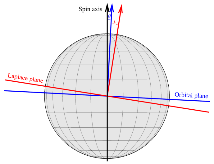
Figure 1: Geometry of Cassini state 1: the three vectors representing spin axis orientation (black), normal to the orbital plane (blue), and normal to the Laplace plane (red) remain coplanar as the orbit precesses around the Laplace plane with a $\sim$300 000-year period. The inclination of Mercury’s orbit with respect to the Laplace plane is represented by the angle $\iota$, which is shown to scale. The tilt of Mercury’s spin axis with respect to the orbit normal is the obliquity $\theta$, which is shown with an exaggeration factor of 100 for clarity.

In a Cassini state, the obliquity has evolved to a value where the spin precession period matches the orbit precession period (Gladman et al.,, 1996). Because the spin precession period and the gravitational torques depend on moment of inertia differences, there is a powerful relationship between the obliquity of a body in a Cassini state and its moments of inertia. Peale, (1976, 1988) wrote

$$K_{1}(\theta)\left(\frac{C-A}{C}\right)+K_{2}(\theta)\left(\frac{B-A}{C}\right)=K_{3}(\theta),$$ (2)

where $K_{1},K_{2},K_{3}$ are functions of the obliquity $\theta$ that involve the orbital eccentricity, inclination with respect to the Laplace plane, mean motion, spin rate, and precession rate. In this equation, the appropriate moment of inertia in the denominator is that of the entire planet, even if the core is molten, because it is hypothesized that the core follows the mantle on the $\sim$300 000-year time scale of the orbital precession.

If we can confirm that Mercury is in a Cassini state, a measurement of the obliquity becomes extremely valuable: it provides a direct constraint on moment of inertia differences and, in combination with degree-2 gravity information, on the polar moment of inertia. A free precession of the spin axis about the Cassini state could, in principle, compromise the determination of the obliquity. However, such free precession would require a recent excitation because the corresponding damping timescale is $\sim$10⁵ y (Peale,, 2005).

2.4 Polar moment of inertia

Absent seismological data, the polar moment of inertia is arguably the most important quantity needed to quantify the interior structure of a planetary body. Peale, (1976, 1988) showed that it is possible to measure the polar moment of inertia $C$ by combining the obliquity with two quantities related to the gravity field. The gravity field of a body of mass $M$ and radius $R$ can be described with spherical harmonics (e.g., Kaula,, 2000). The second-degree coefficients $C_{20}$ and $C_{22}$ in the spherical harmonic expansion are related to the moments of inertia, as follows:

$$C_{20}=-\frac{(C-(A+B)/2)}{MR^{2}},$$ (3)

$$C_{22}=\frac{(B-A)}{4MR^{2}}.$$ (4)

Combining equations (2), (3), and (4), we find

$$\frac{C}{MR^{2}}=(-C_{20}+2C_{22})\frac{K_{1}(\theta)}{K_{3}(\theta)}+4C_{22}\frac{K_{2}(\theta)}{K_{3}(\theta)},$$ (5)

which provides a direct relationship between the obliquity, gravity harmonics, and polar moment of inertia for bodies in Cassini state 1.

To complete Peale’s argument, we determine the polar moment of inertia of the core, which can be done if the core is molten and does not participate in the 88-day librations. To do so, we write the identity

$$\frac{C_{{\rm m}\mbox{{\tiny+}}{\rm cr}}}{C}=\left(\frac{C_{{\rm m}\mbox{{\tiny+}}{\rm cr}}}{B-A}\right)\left(\frac{B-A}{MR^{2}}\right)\left(\frac{MR^{2}}{C}\right),$$ (6)

which yields the moment of inertia of the mantle and crust $C_{{\rm m}\mbox{{\tiny+}}{\rm cr}}$ and, therefore, the moment of inertia of the core $C_{\rm c}=C-C_{{\rm m}\mbox{{\tiny+}}{\rm cr}}$. Two spin state quantities and two gravity quantities provide all the information necessary to determine these values. A measurement of the libration amplitude $\phi_{0}$ provides a direct estimate of the first factor on the right-hand side of equation (6) via equation (1). A measurement of the gravitational harmonic $C_{22}$ provides a direct estimate of the second factor. Measurements of the obliquity, $C_{20}$, and $C_{22}$ yield an estimate of the third factor via equation (5).

The four quantities $\phi_{0},\theta,C_{20},{\rm and}\ C_{22}$ identified by Peale, (1976, 1988) thus provide a powerful probe of the interior structure of the planet.

2.5 Orbital precession

Implementing Peale’s procedure requires precise knowledge of Mercury’s orbital configuration. Whereas the mean motion and orbital eccentricity have been determined from centuries of observations, relatively little attention had been paid to the orientation of the Laplace plane and the orbital precession rate. Yseboodt and Margot, (2006) used a Hamiltonian approach and numerical fits to ephemeris data to determine these ancillary quantities. They showed that the Laplace plane orientation varies due to planetary perturbations on $\sim$10 ky timescales, and they defined an instantaneous Laplace plane valid at the current epoch for the purpose of identifying the position of the Cassini state and interpreting spin-gravity data.

Yseboodt and Margot, (2006) gave the coordinates of the normal to the instantaneous Laplace plane in ecliptic and equatorial coordinates at epoch J2000.0 as

$$\lambda_{\rm inst}=66.6^{\circ},\beta_{\rm inst}=86.725^{\circ},\\$$ (7)

$${\rm RA}_{\rm inst}=273.72^{\circ},{\rm DEC}_{\rm inst}=69.53^{\circ},$$ (8)

where $\lambda$ is ecliptic longitude, $\beta$ is ecliptic latitude, RA is right ascension, and DEC is declination. The uncertainty in the determination is of order $1^{\circ}$, but the orientation of the narrow error ellipse is such that it can affect the interpretation of the spin state data only at a level that is well below that due to measurement uncertainties.

The inclination of Mercury’s orbit with respect to the instantaneous Laplace plane and the orbit precession rate about that plane at the current epoch are $\iota=8.6^{\circ}$ and $\dot{\Omega}=-0.110^{\circ}/{\rm century}$, respectively (Yseboodt and Margot,, 2006). We will use both of these quantities to estimate Mercury’s interior structure in Sections 5 and 7. Stark et al., (2015b) performed an independent analysis and confirmed the values of Yseboodt and Margot, (2006), including the orientation of the instantaneous Laplace plane, the inclination $\iota$, and the precession rate $\dot{\Omega}$. D’Hoedt et al., (2009) used a Hamiltonian approach and found an instantaneous Laplace plane orientation that differs from our preferred value by 1.4^∘.

3 Gravity constraints

3.1 Methods

We are interested in measuring the masses and sizes of planetary bodies because bulk density is a fundamental indicator of composition. In multi-planet systems, masses can be estimated by observing the effects of mutual orbital perturbations, manifested as variations in orbital elements or variations in transit times. Another common mass measurement technique is to determine the orbit of natural satellites.

The most precise mass estimates are obtained by radiometric tracking of a spacecraft while it is in close proximity to the body of interest, typically by using the onboard telecommunications system and a network of ground-based radio telescopes. The geodetic observations are then used to obtain a spherical harmonic expansion of the gravity field and to reconstruct the spacecraft trajectory with high fidelity. In addition to providing high-precision mass estimates, this technique enables the measurement of the spherical harmonic coefficients $C_{20}$ and $C_{22}$, which provide important constraints on interior structure (Section 2.4).

In the following sections, we describe gravity results obtained from tracking the Mariner 10 spacecraft at a frequency of 2.3 GHz (S-band) during three flybys in 1974–1975 and the MESSENGER spacecraft at frequencies of 7.2 GHz uplink and 8.4 GHz downlink (X-band) during the flybys and orbital phase of the mission.

3.2 Mass and density results

The mass, size, and density of Mercury were known with remarkable precision prior to the exploration of the planet by spacecraft. After adding radar measurements to two centuries of optical observations, Ash et al., (1971) fit planetary ephemerides and determined Mercury’s mass to 0.25% fractional uncertainty. They found a value of $6025000\pm 15000$ in inverse solar masses, i.e., $M=(3.300\pm 0.008)\times 10^{23}\ {\rm kg}$, which is almost identical to the modern estimate. Using this measurement and the radar estimate of the average equatorial radius that was available at the time, $R=(2\,439\pm 1)$ km, it was apparent that Mercury’s bulk density was anomalously high, with $\rho=(5\,430\pm 15)\ {\rm kg\,m}^{-3}$. On the basis of their density calculation, Ash et al., (1971) concluded that Mercury must be substantially richer in heavy elements than Earth. The pre-Mariner 10 estimates of mass, size, and density remain in excellent agreement with the MESSENGER results, but spacecraft data have enabled a reduction in uncertainties by a factor of $\sim$50.

Howard et al., (1974) analyzed the tracking data from the first flyby of Mercury by Mariner 10 and obtained a gravitational parameter $GM=(2.2032\pm 0.0002)\times 10^{13}{\rm m}^{3}{\rm s}^{-2}$, where $G$ is the gravitational constant. Analysis of data from all three Mariner 10 flybys yielded $GM=(2.203209\pm 0.000091)\times 10^{13}{\rm m}^{3}{\rm s}^{-2}$(Anderson et al.,, 1987). From more than three years of orbital tracking data of MESSENGER, Mazarico et al., (2014) obtained $GM=(2.203187080\pm 0.000000086)\times 10^{13}{\rm m}^{3}{\rm s}^{-2}$, estimated from a gravity field solution to degree and order 50. An independent analysis to degree and order 40 by Verma and Margot, (2016) yielded $GM=(2.203187404\pm 0.000000090)\times 10^{13}{\rm m}^{3}{\rm s}^{-2}$. When translating the MESSENGER values to a mass estimate, the majority of the uncertainty comes from the $5\times 10^{-5}$ uncertainty in the gravitational constant. With $G=(6.67408\pm 0.00031)\times 10^{-11}{\rm m}^{3}{\rm kg}^{-1}{\rm s}^{-2}$ (Mohr et al.,, 2016), the current best estimate of the mass of Mercury is

$$M=(3.301110\pm 0.00015)\times 10^{23}\ {\rm kg}.$$ (9)

From a combination of laser altimetry (Zuber et al.,, 2012) and radio occultation data, Perry et al., (2015) determined Mercury’s average radius to be

$$R=(2\,439.36\pm 0.02)\ {\rm km},$$ (10)

although the stated radius uncertainty may be optimistic given the sparse sampling of the southern hemisphere. The corresponding bulk density is

$$\rho=(5\,429.30\pm 0.28)\ {\rm kg\,m}^{-3}.$$ (11)

Mercury’s bulk density is similar to that of Earth, $\rho_{\oplus}=5514\ {\rm kg\,m}^{-3}$, despite the different sizes of the two bodies. The pressure $P$ at the center of a homogeneous sphere scales as $P\propto\rho^{2}R^{2}$, so materials in Earth’s interior are more compressed (i.e., denser) than those in Mercury’s interior. If we assume that both planets are made of a combination of a light component (i.e., silicates) and a heavy component (i.e., metals), we can infer from their similar densities and differing sizes that Mercury has a larger metallic component, as recognized by Ash et al., (1971).

3.3 $C_{20}$ and $C_{22}$ results

The first measurements of the $C_{20}$ and $C_{22}$ gravity coefficients were obtained from Mariner 10 data recorded during one equatorial flyby with $\sim$700 km minimum altitude and one polar flyby with $\sim$300 km minimum altitude. Anderson et al., (1987) determined $C_{20}=(-6.0\pm 2.0)\times 10^{-5}$ and $C_{22}=(1.0\pm 0.5)\times 10^{-5}$. These values have large fractional uncertainties because there were only two favorable flybys, but the values are consistent with the most recent MESSENGER results (Mazarico et al.,, 2014; Verma and Margot,, 2016). With the normalization that is commonly used in geodetic studies (Kaula,, 2000; p.7), the Mariner 10 values can also be expressed as $\bar{C}_{20}=C_{20}/\sqrt{5}=(-2.68\pm 0.9)\times 10^{-5}$ and $\bar{C}_{22}=C_{22}/\sqrt{5/12}=(1.55\pm 0.8)\times 10^{-5}$, where the overbar indicates normalized coefficients.

The next opportunity for measurements arose from the three MESSENGER flybys of Mercury in 2008–2009. However, the equatorial geometry of these flybys did not provide adequate leverage to measure $C_{20}$ accurately. Because the Mariner 10 tracking data have been lost, it was not possible to perform a joint solution including both equatorial and polar flybys. For these reasons, Smith et al., (2010) cautioned that their recovery of $\bar{C}_{20}=(-0.86\pm 0.30)\times 10^{-5}$ might not be reliable. However, the equatorial geometry was suitable for an accurate estimate of $\bar{C}_{22}=(1.26\pm 0.12)\times 10^{-5}$.

Data acquired during the orbital phase of the MESSENGER mission provided significantly better sensitivity and lower uncertainties. Smith et al., (2012) analyzed the first six months of data ($>$300 orbits) and found $\bar{C}_{20}=(-2.25\pm 0.01)\times 10^{-5}$ and $\bar{C}_{22}=(1.25\pm 0.01)\times 10^{-5}$, where the error bars represent a calibrated uncertainty that is about 10 times the formal uncertainty of the fit. An independent analysis of the same data by Genova et al., (2013) confirmed these results. More recently, Mazarico et al., (2014) analyzed three years of data (2275 orbits) and estimated a gravity field solution to degree and order 50. This solution yielded an order-of-magnitude improvement in the calibrated uncertainties in $C_{20}$ and $C_{22}$: $\bar{C}_{20}=(-2.2505\pm 0.001)\times 10^{-5}$ and $\bar{C}_{22}=(1.2454\pm 0.001)\times 10^{-5}$. An independent analysis by Verma and Margot, (2016) confirmed these values to better than 0.4%.

The unnormalized quantities that we use in equations (3–6) are based on the Mazarico et al., (2014) values: $C_{20}=(-5.0323\pm 0.0022)\times 10^{-5}$ and $C_{22}=(0.8039\pm 0.0006)\times 10^{-5}$. The $J_{2}/C_{22}=-C_{20}/C_{22}$ value of 6.26 is distinct from the equilibrium value of 7.86 for a body in a 3:2 spin-orbit resonance with the current value of the orbital eccentricity (Matsuyama and Nimmo,, 2009), indicating that Mercury is not in hydrostatic equilibrium.

3.4 $k_{2}$ results

In addition to the static gravity field, Mazarico et al., (2014) also solved for the time-variable degree-2 potential which captures the tidal forcing due to the Sun. The tidal forcing is parameterized by the Love number $k_{2}$ (Section 8.1). Mazarico et al., (2014) obtained an estimate of $k_{2}=0.451\pm 0.014$. However, because of potential mismodeling and systematic effects in the analysis, they could not rule out a wider range of values ($0.43-0.50$). The preferred value of Verma and Margot, (2016) is $k_{2}=0.464\pm 0.023$. They, too, encountered a wider range of best-fit values ($0.420-0.465$) in various trials. The weighted mean of these two estimates is $k_{2}=0.455\pm 0.012$. These estimates are within the expected range from theoretical studies (Van Hoolst and Jacobs,, 2003; Van Hoolst et al.,, 2007; Rivoldini et al.,, 2009) and from predictions of interior models informed by MESSENGER data and Earth-based radar data (Padovan et al.,, 2014).

4 Spin-state constraints

Most of the quantities necessary to implement Peale’s method of probing Mercury’s interior were known when he wrote his paper in 1976. The mass, size, and density had been determined to $<1\%$ precision prior to the arrival of Mariner 10, the data from which confirmed and improved the ground-based estimates (Section 3). Values of the second-degree gravity coefficients $C_{20}$ and $C_{22}$ had also been determined, albeit with substantial uncertainties. In contrast, there were no satisfactory measurements of the spin state. Librations had not been detected, and the best spacecraft determination of the orientation of the rotation axis had a 50% error ellipse of $\pm 2.6^{\circ}$ by $\pm 6.5^{\circ}$ (Klaasen,, 1976), about three orders of magnitude short of the required precision. Peale, (1976) speculated that measurement of the obliquity and libration angles ($\theta$ and $\phi_{0}$) would “almost certainly require rather sophisticated instrumentation on the surface of the planet.” Fortunately, the measurements were obtained with Earth-based instruments as well as instruments aboard the MESSENGER orbiter.

4.1 Methods

Three observational methods have been used to measure Mercury’s spin state: Earth-based radar observations, joint analysis of MESSENGER laser altimetry tracks and stereo-derived digital terrain models, and MESSENGER radio tracking observations. All three yielded estimates of Mercury’s obliquity, but only the first two have yielded libration measurements so far. Another important distinction between these methods is that the first two measure the spin state of the rigid outer part of the planet, i.e., the lithosphere, whereas the gravity-based analyses are sensitive to the rotation of the entire planet.

The spin state of Mercury can be characterized to high precision with an Earth-based radar technique that relies on the theoretical ideas of Holin, (1988, 1992). He showed that radar echoes from solid planets can display a high degree of correlation when observed by two receiving stations with appropriate positions in four-dimensional space-time. Normally each station observes a specific time history of fluctuations in the echo power (also known as speckles), and the signals recorded at separate antennas do not correlate. But during certain times on certain days of the year, the antennas become suitably aligned with the speckle trajectory, which is tied to the rotation of the observed planet (Figure 2).

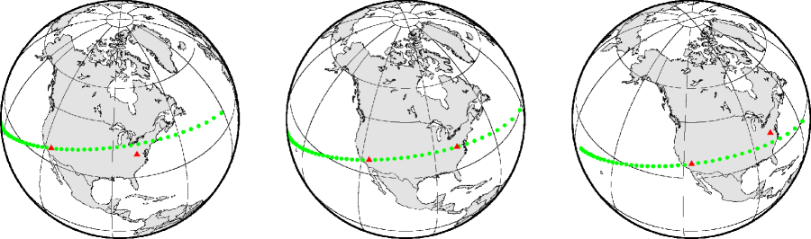
Figure 2: Radar echoes from Mercury sweep over the surface of the Earth. Diagrams show the trajectory of the speckles one hour before (left), during (center), and one hour after (right) the epoch of maximum correlation. Echoes from two receive stations (red triangles) exhibit a strong correlation when the antennas are suitably aligned with the trajectory of the speckles (green dots shown with a 1-s time interval). From Margot et al., (2012).

During these brief ($\sim$10–20 s) time intervals a cross-correlation of the two echo time series yields a high score at a certain value of the time lag ($\sim$5–10 s). The epoch at which the high correlation occurs provides a strong constraint on the orientation of the spin axis. The time lag at which the high correlation occurs provides a direct measurement of the spin rate. Margot et al., (2007, 2012) illuminated Mercury with monochromatic radiation (8560 MHz, 450 kW) from the Deep Space Network (DSN) 70-m antenna in Goldstone, California (DSS-14), and recorded the speckle patterns as they swept over two receiving stations (DSS-14 and the 100-m antenna in Green Bank, West Virginia). They obtained measurements of the instantaneous spin state of Mercury at 35 epochs between 2002 and 2012, from which they inferred both obliquity and libration angles.

Stark et al., (2015a) combined imaging (Hawkins et al.,, 2007) and laser altimetry (Cavanaugh et al.,, 2007) data obtained by MESSENGER during orbital operations to independently measure the spin state of Mercury. The basic idea is to produce digital terrain models (DTMs) from stereo analysis of the imaging data and to coregister the laser altimetry profiles to the DTMs (Stark et al.,, 2015c). During the coregistration step, a rotational model is adjusted in a way that minimizes the radial height differences between the two data sets. This adjustment enables the recovery of the spin axis orientation, which yields the value of the obliquity. It also enables the recovery of the amplitude of the physical librations because the laser profiles sample the topography of the surface at different phases of the libration cycle. In practice, Stark et al., (2015a) produced 165 individual gridded DTMs from thousands of images of the surface. Their DTMs cover $\sim$50% of the northern hemisphere of Mercury with a grid spacing of 222 m/pixel, an effective horizontal resolution of 3.8 km, and an average height error of 60 m. For the coregistration step, they used 2325 laser profiles from three years of Mercury Laser Altimeter (MLA) observations. The laser altimetry data have a spacing between footprints that varied between 170 m and 440 m and a nominal ranging accuracy of 1 m.

The third method for estimating the spin state of Mercury is to adjust a rotational model of the planet during analysis of the radio tracking data (Section 3). Mazarico et al., (2014) and Verma and Margot, (2016) analyzed three years of radio science data and produced estimates of the spin axis orientation. The detection of the physical librations with this technique is possible, but measuring the libration amplitude accurately remains challenging.

4.2 Obliquity results

Analysis of the Earth-based radar data yielded an estimate of the obliquity $\theta=(2.042\pm 0.08)\ {\rm arcminutes}$, where the adopted one-standard-deviation uncertainty corresponds to 5 arcseconds (Margot et al.,, 2012). Remarkably, the analysis of the spacecraft imaging and laser altimetry data, a completely independent data set, yielded an almost identical (0.6%) estimate of $(2.029\pm 0.085)\ {\rm arcminutes}$, with similar uncertainties (Stark et al.,, 2015a). The weighted mean of these two estimates is $\theta=(2.036\pm 0.058)$ arcminutes.

The best-fit spin axis orientation at epoch J2000.0 from analysis of the radar data is at equatorial coordinates (281.0103^∘, 61.4155^∘) and ecliptic coordinates (318.2352^∘, 82.9631^∘) in the corresponding J2000 frames (Margot et al.,, 2012). The MESSENGER DTM and laser altimetry results are within 0.8 arcseconds, at equatorial coordinates (281.0098^∘, 61.4156^∘) and ecliptic coordinates (318.2343^∘, 82.9633^∘) (Stark et al.,, 2015a).

Radio science tracking data can be used to estimate the orientation of the axis about which Mercury’s gravity field rotates, which is not necessarily aligned with the axis about which the lithosphere rotates. Mazarico et al., (2014) and Verma and Margot, (2016) used this technique and reported obliquities of $(2.06\pm 0.16)\ {\rm and\ }(1.88\pm 0.16)\ {\rm arcminutes}$, respectively. These results are consistent with those obtained by Margot et al., (2012) and Stark et al., (2015a), albeit with uncertainties that are twice as large (Figure 3).

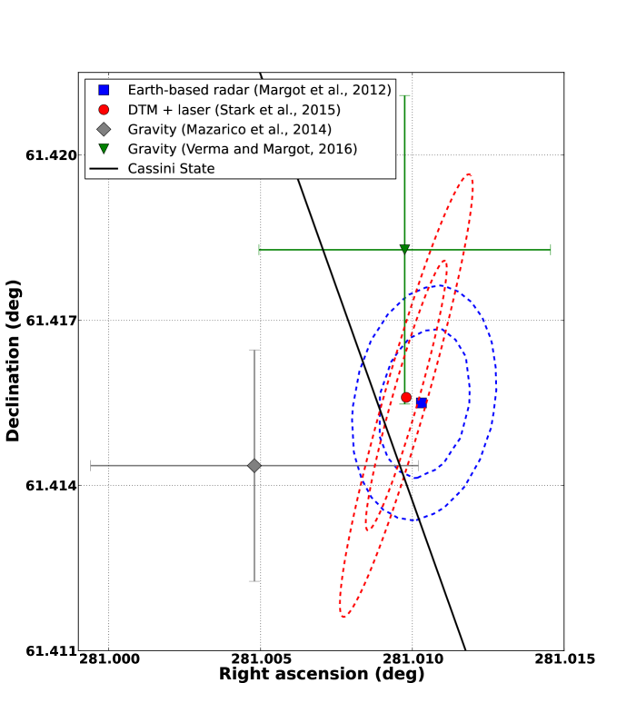
Figure 3: Orientation of the spin axis of Mercury obtained by three different techniques. The Earth-based radar results and the MESSENGER DTM and laser altimetry results are shown with contours representing the 1- and 2-standard deviation uncertainty regions. The gravity results are shown with error bars representing the formal uncertainties of the fit multiplied by 10. The oblique line shows the predicted location of Cassini state 1 at epoch J2000.0 from the analysis of Yseboodt and Margot, (2006). Points to the left and right of the line lead and lag the Cassini state, respectively.

Margot et al., (2007) provided observational evidence that Mercury is in or very near Cassini state 1, an important condition for the success of Peale’s procedure. The current best-fit values place the radar-based and MESSENGER-based poles within 2.7 and 1.7 arcseconds of the Cassini state, respectively (Figure 3), confirming that Mercury closely follows the Cassini state. There are several possible interpretations for the imperfect agreement: (1) given the 5–6 arcsecond uncertainty in spin axis orientation, Mercury may in fact be in the exact Cassini state, (2) Mercury may also be in the exact Cassini state if our knowledge of the location of that state is incorrect, which is possible because it is difficult to determine the exact Laplace pole orientation, (3) Mercury may lag the exact Cassini state by a few arcseconds, (4) Mercury may lead the exact Cassini state, although this seems less likely on the basis of the evidence at hand. Measurements of the offset between the spin axis orientation and the Cassini state location have been used to place bounds on energy dissipation due to solid-body tides and core-mantle interactions in the Moon (Yoder,, 1981; Williams et al.,, 2001). However, the interpretation of an offset from the Cassini state at Mercury is complicated by the influence of various core-mantle coupling mechanisms (Peale et al.,, 2014) and the presence of an inner core (Peale et al.,, 2016).

4.3 Libration results

Analysis of Earth-based radar observations obtained at 18 epochs between 2002 and 2006 yielded measurements of Mercury’s instantaneous spin rate that revealed an obvious libration signature with a period of 88 days (Margot et al.,, 2007). From these data and the Mariner 10 estimate of $C_{22}$ in equation (6), it was possible to show with 95% confidence that $C_{{\rm m}\mbox{{\tiny+}}{\rm cr}}/C$ is smaller than unity. These results provided direct observational evidence that Mercury has a molten outer core (Margot et al.,, 2007). Measurements of Mercury’s magnetic field prior to the radar observations had provided inconclusive suggestions about the nature of Mercury’s core. A dynamo mechanism involving motion in an electrically conducting molten outer core was the preferred explanation (Ness et al.,, 1975; Stevenson,, 1983), but alternative theories that did not require a liquid core, such as remanent magnetism in the crust, could not be ruled out (Stephenson,, 1976; Aharonson et al.,, 2004).

Earth-based radar observations continued during the flyby and orbital phases of MESSENGER. By 2012, measurements at 35 epochs had been obtained (Figure 4). One can fit a libration model (Margot,, 2009) to these data and derive the value of $(B-A)/C_{{\rm m}\mbox{{\tiny+}}{\rm cr}}$. Margot et al., (2012) found a value of $(B-A)/C_{{\rm m}\mbox{{\tiny+}}{\rm cr}}=(2.18\pm 0.09)\times 10^{-4}$, which corresponds to a libration amplitude $\phi_{0}$ of $(38.5\pm 1.6)$ arcseconds, or a longitudinal displacement at the equator of 450 m.

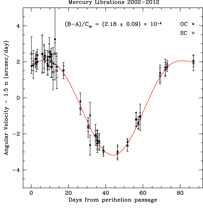
Figure 4: Mercury 88-day librations revealed by 35 instantaneous spin rate measurements obtained with Earth-based radar between 2002 and 2012. The vertical axis represents deviations of the angular velocity from the exact resonant rate of 3/2 times the mean orbital motion $n$. The measurements with their one-standard-deviation errors are shown in black. OC and SC represent measurements in two orthogonal polarizations (opposite-sense circular and same-sense circular, respectively). A numerical integration of the torque equation is shown in red. The flat top on the angular velocity curve near pericenter is due to the momentary retrograde motion of the Sun in the body-fixed frame and corresponding changes in the torque. The amplitude of the libration curve is determined by a one-parameter least-squares fit to the observations, which yields a value of $(B-A)/C_{m+cr}=(2.18\pm 0.09)\times 10^{-4}$. From Margot et al., (2012).

Stark et al., (2015a) analyzed three years of MESSENGER DTM and laser altimetry data and found a libration amplitude of $(38.9\pm 1.3)$ arcseconds, which corresponds to $(B-A)/C_{{\rm m}\mbox{{\tiny+}}{\rm cr}}=(2.206\pm 0.074)\times 10^{-4}$. This estimate is in excellent agreement (1%) with the Earth-based radar value, giving confidence in the robustness of the results obtained by two independent techniques. The weighted means of these estimates are $(B-A)/C_{{\rm m}\mbox{{\tiny+}}{\rm cr}}=2.196\pm 0.057$ and $\phi_{0}=(38.7\pm 1.0)$ arcseconds.

4.4 Average spin rate

Questions remain about the precise spin behavior of Mercury, both in terms of its average spin rate and the presence of additional libration signatures. There are reasons to believe that longitudinal librations with periods of 2–20 y exist, either because of planetary perturbations (Peale et al.,, 2007; Dufey et al.,, 2008; Peale et al.,, 2009; Yseboodt et al.,, 2010) or because of internal couplings and forcings (Veasey and Dumberry,, 2011; Dumberry,, 2011; Van Hoolst et al.,, 2012; Yseboodt et al.,, 2013; Koning and Dumberry,, 2013; Dumberry et al.,, 2013). However, the addition of long-term libration components to the rotational model was not found to improve fits to the 2002–2012 radar data (Margot et al.,, 2012; Yseboodt et al.,, 2013). The duration of the MESSENGER data sets is not sufficiently long to detect a long-term libration signature, for which the primary period is expected to be $\sim$12 y. Therefore, Mazarico et al., (2014) and Stark et al., (2015a) did not attempt to fit for long-term librations. Instead, they obtained estimates of Mercury’s average spin rate over the time span of the MESSENGER mission. Their estimates differ substantially from one another and from the expected mean resonant spin rate (Fig. 5). One possible explanation for the discrepancy between theoretical and observational estimates is that the MESSENGER estimates are based on a 3- or 4-year period that represents only a small fraction of the long-term libration cycle.

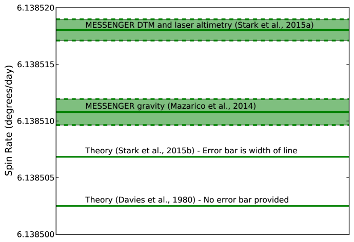
Figure 5: Theoretical and observational estimates of Mercury’s mean resonant spin rate. The Davies et al., (1980) value was adopted in the latest report of the International Astronomical Union Working Group on Cartographic Coordinates and Rotational Elements (Archinal et al.,, 2011).

5 Two- and three-layer structural models

5.1 Governing equations

The bulk density $\rho=M/V$ of a planetary body of mass $M$ and volume $V$ is an important indicator of composition, but it contains no information about the radial distribution of the material in the interior. Because we seek to calculate the radial density profile $\rho(r)$, we write expressions for the mass and bulk density of a spherically symmetric body of radius $R$ that highlight the mass contributions from concentric spherical shells of width $dr$:

$$M=4\pi\int_{0}^{R}{\rho(r)r^{2}dr},$$ (12)

$$\rho=\frac{3}{R^{3}}\int_{0}^{R}{\rho(r)r^{2}dr}.$$ (13)

We write similar expressions for the polar moment of inertia $C$ and its normalized value $\widetilde{C}$:

$$C=\frac{8\pi}{3}\int_{0}^{R}{\rho(r)r^{4}dr},$$ (14)

$$\widetilde{C}=\frac{C}{MR^{2}}=\frac{2}{\rho R^{5}}\int_{0}^{R}{\rho(r)r^{4}dr}.$$ (15)

We first consider a two-layer model where a mantle with constant density $\rho_{\rm m}$ overlays a core with constant density $\rho_{\rm c}$ and radius $R_{\rm c}$. In a gravitationally stable configuration, $\rho_{\rm c}>\rho_{\rm m}$. We use equations (13) and (15) to derive the analytical expressions for bulk density and normalized moment of inertia for this two-layer model:

$$\rho = \rho_{\rm c}\alpha^{3}+\rho_{\rm m}\left(1-\alpha^{3}\right),$$ (16)

$$\widetilde{C} = \frac{2}{5}\left[\frac{\rho_{\rm c}}{\rho}\alpha^{5}+\frac{\rho_{\rm m}}{\rho}\left(1-\alpha^{5}\right)\right],$$ (17)

where we have have used $\alpha=R_{\rm c}/R$ for ease of notation. This system is underdetermined, because there are three unknowns ($\rho_{\rm c}$, $\rho_{\rm m},$ and $R_{\rm c}$) and only two observables ($\rho$ and $\widetilde{C}$). Even in the case of an oversimplified two-layer model, it is not possible to find a solution without making an additional assumption or securing an additional observable. For example, one could proceed by making an educated guess about the density of the mantle from measurements of the composition of the surface. A more rigorous approach is to obtain an additional observable that depends directly on the density of the mantle. We rely on Peale’s procedure and the fact that Mercury is in a Cassini state (Section 4.2) to provide such an observable, the polar moment of inertia of the mantle plus crust as given by equation (6). For the two-layer model, this expression reduces to

$$\frac{C_{{\rm m}\mbox{{\tiny+}}{\rm cr}}}{C} = \frac{\rho_{\rm m}\left(1-\alpha^{5}\right)}{\rho_{\rm c}\alpha^{5}+\rho_{\rm m}\left(1-\alpha^{5}\right)}.$$ (18)

5.2 Moment of inertia results

Peale’s formalism (Section 2.4) enabled a determination of Mercury’s polar moment of inertia. Margot et al., (2012) combined measurements of the obliquity and librations with gravity data and found $\widetilde{C}=0.346\pm 0.014$. Stark et al., (2015a) also measured $\theta$ and $\phi_{0}$, and found $\widetilde{C}=0.346\pm 0.011$. A uniform density sphere has $\widetilde{C}=0.4$, and a body with a density profile that increases with depth has $\widetilde{C}<0.4$. The Moon, with $\widetilde{C}\simeq 0.393$ (Williams et al.,, 1996), is nearly homogeneous, whereas the Earth, with $\widetilde{C}=0.3307$ (Williams,, 1994), has a substantial concentration of dense material near the center. Likewise, Mercury’s $\widetilde{C}$ value suggests the presence of a dense metallic core.

The moment of inertia of Mercury’s mantle and crust is also available from spin and gravity data (Equation 6). Margot et al., (2012) found $C_{{\rm m}\mbox{{\tiny+}}{\rm cr}}/C=0.431\pm 0.025$ and Stark et al., (2015a) found $C_{{\rm m}\mbox{{\tiny+}}{\rm cr}}/C=0.421\pm 0.021$.

Weighted means of the Margot et al., (2012) and Stark et al., (2015a) results provide the most reliable estimates to date of the moments of inertia. We find

$$\widetilde{C}=\frac{C}{MR^{2}}=0.346\pm 0.009,$$ (19)

$$\frac{C_{{\rm m}\mbox{{\tiny+}}{\rm cr}}}{C}=0.425\pm 0.016.$$ (20)

An error budget similar to that computed by Peale, (1981, 1988) demonstrates that the dominant sources of uncertainties in the moment of inertia values can be attributed to spin quantities. Uncertainties arising from gravitational harmonics, tides, and orbital elements are at least an order of magnitude smaller (Noyelles and Lhotka,, 2013; Baland et al.,, 2017). Further improvements to our knowledge of Mercury’s moments of inertia therefore require better estimates of obliquity and libration amplitude. Such improved estimates may also enable a determination of the tidal quality factor $Q$ (Baland et al.,, 2017).

5.3 Two-layer model results

Using equations (16–18) and estimates of bulk density (11), $\widetilde{C}$ (19), and $C_{\rm m+cr}/C$ (20), we infer

$$R_{\rm c}/R = 0.8209,\ i.e.,\quad R_{\rm c} = 2\,002\ {\rm km},\$$ (21)

$$\rho_{\rm c}/\rho = 1.3344,\ i.e.,\quad\rho_{\rm c} = 7\,245\ {\rm kg\,m}^{-3},\$$ (22)

$$\rho_{\rm m}/\rho = 0.5861,\ i.e.,\quad\rho_{\rm m} = 3\,182\ {\rm kg\,m}^{-3}.$$ (23)

The results obtained with the two-layer model are within one standard deviation of the results of more elaborate, multi-layer models that take into account mineralogical, geochemical, and rheological constraints on the composition and physical properties of the interior (Hauck et al.,, 2013; Rivoldini and Van Hoolst,, 2013; Section 7). Figure 6 illustrates the consistency of the two-layer solution (star) and of the multi-layer models of Hauck et al., (2013) (error bars). The two-layer model results are also consistent with results from multi-layer models that consider the total contraction of the planet (Knibbe and van Westrenen,, 2015).

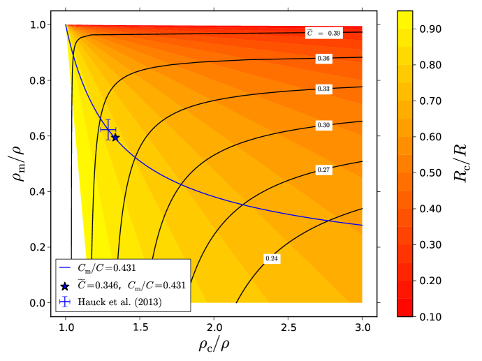
Figure 6: Mantle density versus core density showing the consistency of the two-layer model results (star) with those of more elaborate, multi-layer models (error bars). The position of the star corresponds to values of $\widetilde{C}=0.346$ and $C_{{\rm m}\mbox{{\tiny+}}{\rm cr}}/C=0.431$ (Margot et al.,, 2012). Error bars correspond to the one-standard-deviation intervals for $\rho_{\rm c}/\rho$ and $\rho_{\rm m}/\rho$ obtained by Hauck et al., (2013). The background color map indicates the value $R_{\rm c}/R$ in the two-layer model. Black curves illustrate models with various values of the normalized moment of inertia $\widetilde{C}$. The blue curve traces the locus of two-layer models with $C_{{\rm m}\mbox{{\tiny+}}{\rm cr}}/C=0.431$.

All points shown on Figure 6 are consistent with Mercury’s bulk density $\rho$. Knowledge of the normalized moment of inertia $\widetilde{C}$ restricts acceptable models to a black, constant-$\widetilde{C}$ curve. The resulting degeneracy corresponds to the underdetermined system of equations (13) and (15). Knowledge of the moment of inertia of the mantle further restricts acceptable models to the blue curve. The intersection of the $\widetilde{C}=0.346$ black curve (not shown) and of the $C_{\rm m+cr}/C=0.431$ blue curve yields the two-layer model solution.

Although three observables ($\rho$, $\widetilde{C}$, and $C_{{\rm m}\mbox{{\tiny+}}{\rm cr}}/C$) can be used to reliably estimate the parameters of a two-layer model (core size, core density, and mantle density), they provide no information about additional phenomena related to the origin, evolution, and present physical state of the planet (e.g., mineralogical composition of the mantle, composition of the core, presence of a solid inner core). Additional insight can be obtained with more elaborate three-layer and multi-layer models.

5.4 Three-layer models

We now consider a three-layer model with core, mantle, and crust of density $\rho_{\rm cr}$. We express the core and mantle radii as fractions of the planetary radius, $\alpha=R_{\rm c}/R$ and $\beta=R_{\rm m}/R$. With this notation, we can write the bulk density, moment of inertia, and the moment of inertia of the outer solid shell as follows:

$$\rho = \rho_{\rm c}\alpha^{3}+\rho_{\rm m}\left(\beta^{3}-\alpha^{3}\right)+\rho_{\rm cr}\left(1-\beta^{3}\right),$$ (24)

$$\widetilde{C} = \frac{2}{5}\left[\frac{\rho_{\rm c}}{\rho}\alpha^{5}+\frac{\rho_{\rm m}}{\rho}\left(\beta^{5}-\alpha^{5}\right)+\frac{\rho_{\rm cr}}{\rho}\left(1-\beta^{5}\right)\right],$$ (25)

$$\frac{C_{{\rm m}\mbox{{\tiny+}}{\rm cr}}}{C} = \frac{\rho_{\rm m}\left(\beta^{5}-\alpha^{5}\right)+\rho_{\rm c}\left(1-\beta^{5}\right)}{\rho_{\rm c}\alpha^{5}+\rho_{\rm m}\left(\beta^{5}-\alpha^{5}\right)+\rho_{\rm c}\left(1-\beta^{5}\right)}.$$ (26)

This system of equations has 5 unknowns and 3 observables. If we assume a crustal thickness value $h_{\rm cr}$ (i.e., $\beta$) and a crustal density value $\rho_{\rm cr}$, the system of equations (24)-(26) can be solved. The thickness of the crust of Mercury has been estimated from the combined analysis of gravity and topography data (Mazarico et al.,, 2014; Padovan et al.,, 2015; James et al.,, 2015). The density of the crust $\rho_{\rm cr}$ can be estimated from the measured composition of the surface of Mercury (e.g., Padovan et al.,, 2015).

We use the results of Padovan et al., (2015) and consider two end-member cases: a crust that is low-density and thin ($\rho_{\rm cr}=2\,700$ ${\rm kg\,m}^{-3}$, $h_{\rm cr}=17$ ${\rm km}$) and a crust that is high-density and thick ($\rho_{\rm cr}=3\,100$ ${\rm kg\,m}^{-3}$, $h_{\rm cr}=53$ ${\rm km}$). Compared with the two-layer model, the inferred radius of the core is almost unaffected by the inclusion of the crust, and the densities of the mantle and core change by less than 1%. This result can be explained by the small volume of the crust and the fact that its density is lower than that of the underlying layers. Consequently, the presence of the crust does not change the values of $\rho,$ $\widetilde{C}$, and $C_{\rm m+cr}/C$ appreciably.

Another possible three-layer model includes a solid inner core, a liquid outer core and a mantle. However, the composition of the core is not well constrained, and the system of equations (24)–(26) cannot be solved. To make further progress, we build multi-layer models (Section 7) that include additional, indirect constraints from the observed composition of the surface (Section 6) and from assumptions about interior properties guided by laboratory experiments. We then incorporate constraints that arise from the measurement of planetary tides (Section 8).

6 Compositional constraints

Measurements of the surface chemistry of Mercury by the MESSENGER spacecraft have provided important information on the composition of the interior (e.g., Chapter 2). Observations by the X-Ray Spectrometer (XRS) and Gamma-Ray and Neutron Spectrometer (GRNS) instruments have demonstrated that Mercury’s surface has a low ($<$2.5 wt %) abundance of iron (Nittler et al.,, 2011; Evans et al.,, 2012; Weider et al.,, 2014; Chapter 2). This surface abundance, if also reflective of the mantle concentration of Fe (Robinson and Taylor,, 2001), implies that the bulk density of the mantle is only modestly higher than those of the magnesium end-members of the likely major minerals, e.g., orthopyroxene enstatite with a density of 3 200 ${\rm kg\,m}^{-3}$ (Smyth and McCormick,, 1995). From the application of a normative mineralogy to the measured surface elemental abundances (Weider et al.,, 2015), Padovan et al., (2015) inferred grain densities for the crust of Mercury between 3 000 and 3 100 ${\rm kg\,m}^{-3}$, a result driven primarily by the low Fe abundance. In addition to the low surface Fe abundance, Mercury has relatively large concentrations of sulfur in surface materials (Nittler et al.,, 2011; Chapter 2). When taken with the Fe observations, the measured S abundance of $\sim$1.5–2.3 wt % in the crust implies strongly chemically reducing conditions (i.e., oxygen fugacities 2.6 to 7.3 log₁₀ units below the iron-wüstite buffer) in Mercury’s interior during the partial melting that yielded these materials (Nittler et al.,, 2011; McCubbin et al.,, 2012; Zolotov et al.,, 2013). This inference is consistent with some pre-MESSENGER expectations (e.g., Wasson,, 1988; Burbine et al.,, 2002; Malavergne et al.,, 2010). Two consequences of such reducing conditions are that, during global differentiation, S is more soluble in silicate melts that later crystallize as sulfides within the dominantly silicate material, and Si is more soluble in metallic Fe that segregates to the core. As a result, a wide range of core compositions has been considered when investigating Mercury’s internal structure. The pressure, temperature, and compositional conditions relevant to Mercury’s core have been tabulated by Rivoldini et al., (2009) and Hauck et al., (2013).

As Mercury’s large bulk density has long implied, the planet has a large metallic core dominated by Fe that is likely alloyed with one or more lighter elements. Previous investigations focused on S as the major alloying element for Mercury’s core (e.g., Stevenson et al.,, 1983; Schubert et al.,, 1988; Harder and Schubert,, 2001; Van Hoolst and Jacobs,, 2003; Hauck et al.,, 2007; Riner et al.,, 2008; Rivoldini et al.,, 2009; Dumberry and Rivoldini,, 2015) because of its cosmochemical abundance and the greater availability of thermodynamic data. Sulfur has a strong effect on the density of Fe alloys, much greater than silicon or carbon for a given abundance. Additionally, S can lower the melting point of Fe alloys by hundreds of K, which is important for maintaining a liquid outer core, and it is relatively insoluble in solid Fe, the crystallizing phase in Fe-rich Fe–S systems. The latter property is important because it leads to a nearly pure Fe inner core and an outer core that is progressively enriched in S as a function of inner core growth.

For the most chemically reduced end-members of Mercury’s inferred interior compositions, it is likely that Si is the primary, or sole, light alloying element in the metallic core. Alloys of Fe and Si have a markedly different behavior from Fe–S alloys in that they display a solid solution with a narrow phase loop, i.e., a narrow region between solidus and liquidus curves at high pressure (Kuwayama and Hirose,, 2004). As a consequence, compositional differences between the potential solids and liquids in the core are much more limited, and thus density contrasts across the inner core boundary are smaller than for Fe–S core compositions. Silicon also has a smaller effect on the density and compressibility of Fe–Si alloys than does S, with the consequence that more Si than S is required to achieve the same density reduction relative to pure Fe. Data on the equation of state of solid Fe–Si alloys are more plentiful than for liquid Fe–Si alloys, particularly at higher pressures, though the data are sufficient to construct models of Mercury’s internal structure (Hauck et al.,, 2013). Due to the narrow phase loop and more limited melting point depression induced by Si in Fe alloys (e.g., Kuwayama and Hirose,, 2004), inner core growth could be more extensive in Fe–Si systems than in S-bearing core alloys.

Over the range of inferred oxygen fugacities of 2.6 to 7.3 log₁₀ units below the iron-wüstite buffer for Mercury’s interior, an alloy of Fe with both S and Si is likely in the core (Malavergne et al.,, 2010; Smith et al.,, 2012; Hauck et al.,, 2013; Namur et al.,, 2016b). Indeed, metal-silicate partitioning experiments motivated by the surface compositions measured by MESSENGER indicate that S and Si are likely both present in materials that make up Mercury’s core (Chabot et al.,, 2014; Namur et al.,, 2016b). Unfortunately, data for the thermodynamic and thermoelastic properties of ternary alloys at high pressure are more limited than for their binary end-members. Experiments on the behavior of super-liquidus Fe–S–Si alloys have demonstrated large fields of two-liquid immiscibility (e.g., Sanloup and Fei,, 2004; Morard and Katsura,, 2010) with separate S-rich and Si-rich liquids at pressures relevant to Mercury’s outermost core. Such immiscibility, if present in Mercury’s core, would lead to a separation of phases with more S-rich liquids at the top of the core and Si-rich liquids deeper. In this situation, it is possible to assume end-member behavior in two separate compositional layers within the core and calculate properties separately for each layer (e.g., Smith et al.,, 2012; Hauck et al.,, 2013). However, liquid immiscibility in this system at higher pressures requires rather substantial amounts of both Si and S, which may or may not be appropriate. Experiments by Chabot et al., (2014) indicate a trade-off between Si and S in Mercury’s metallic core that only minimally overlaps with current understanding of the Fe–S–Si liquid-liquid immiscibility phase field. Those results suggest that a mixture of Fe, S, and Si may be more likely. More recent work by Namur et al., (2016b), however, suggests that Mercury’s core conditions may belong to the immiscible liquid field. In this case, Mercury’s core may contain enough S for an FeS layer that is anywhere from negligibly thin to 90 km thick, depending on bulk S content of the planet. Regardless, the range of likely compositions for Mercury’s core lies somewhere between an Fe-Si end-member and a (possibly segregated) mix of Fe, Si, and S.

7 Multi-layer structural models

We now wish to construct internal structure models with many layers in order to better match the gravity, spin state, and compositional constraints. We extend the approach of the two- and three-layer models (Section 5) to N-layer models with the goal of reproducing both discontinuous and continuous variations in density with depth. Such variations are expected on the basis of pressure-induced changes in the density of materials. For each material, an equation of state (EOS) describes the density as a function of pressure, temperature, and composition. Pressure variations inside Mercury’s core require an EOS, but the range of pressures expected across Mercury’s thin silicate shell is relatively small. As a result, some models do not include an EOS for the silicate layer (Hauck et al.,, 2007, 2013; Smith et al.,, 2012; Dumberry and Rivoldini,, 2015), although some models do (Harder and Schubert,, 2001; Riner et al.,, 2008; Rivoldini et al.,, 2009; Rivoldini and Van Hoolst,, 2013; Knibbe and van Westrenen,, 2015). Multi-layer models provide an opportunity to reduce some of the non-uniqueness of simpler models through application of knowledge of the interior (e.g., potential core compositions) (Hauck et al.,, 2013; Rivoldini and Van Hoolst,, 2013). They also enable investigations related to the structure of the core (Hauck et al.,, 2013; Dumberry and Rivoldini,, 2015; Knibbe and van Westrenen,, 2015) and the implications for the planet’s thermal evolution and magnetic field generation.

7.1 Elements of the model

Like two- and three-layer models, N-layer models consist of a series of layers defined by their composition and physical state. In contrast to simpler models, most of the geophysically defined layers in N-layer models are further subdivided into hundreds or thousands of sublayers. The sublayers provide for a smoother variation of density within the geophysically defined layers. Sublayer properties are functionally defined by the relevant EOS (Hauck et al.,, 2013; Rivoldini and Van Hoolst,, 2013).

The basic internal organization of N-layer models is illustrated in Figure 7. The metallic core is divided into a solid inner core and a liquid outer core. Core densities vary according to the EOS. The solid outer portion of the planet is divided into one or more solid outer layers, most commonly with densities that are constant throughout their depth extent. Several models employ a traditional division of the solid outer shell into a crust and a mantle (Hauck et al.,, 2013; Rivoldini and Van Hoolst,, 2013; Dumberry and Rivoldini,, 2015; Knibbe and van Westrenen,, 2015). Here, as did Hauck et al., (2013), we define up to three layers within the solid outermost portion of the planet: a basal layer at the bottom the mantle, a mantle, and a silicate crust. The presence of a basal layer was suggested as a way to reconcile the low amounts of Fe observed at the planet’s surface with the high bulk density of Mercury’s outer solid shell inferred from spin and gravity data (Smith et al.,, 2012; Hauck et al.,, 2013). Evidence for deep compensation of domical swells on Mercury (James et al.,, 2015) also suggests that compositional variations deep within the solid outer shell are present, at least regionally.

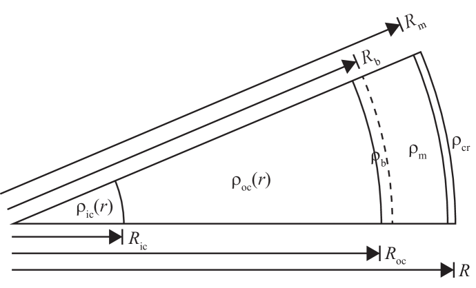
Figure 7: Schematic representation of the internal layers of Mercury in models with detailed sub-layering aimed at capturing density variations due to changes in pressure, temperature, and composition with depth. Specific radii mark the transitions between layers, as follows: $R_{\rm ic}$ between solid inner core and liquid outer core, $R_{\rm oc}$ between liquid outer core and the solid outer shell of the planet, $R_{\rm b}$ between a compositionally distinct layer at the base of the mantle and the overlying mantle, and $R_{\rm m}$ between mantle and crust. The radius of the planet is $R$. The radially varying densities of the inner core and outer core are $\rho_{\rm ic}(r)$ and $\rho_{\rm oc}(r)$, respectively. The constant densities of any basal layer, mantle, and crust are $\rho_{\rm b}$, $\rho_{\rm m}$, and $\rho_{\rm cr}$, respectively.

7.2 Governing equations

Any internal structure model for Mercury must be consistent with three quantities: the bulk density of the planet, the normalized moment of inertia $\widetilde{C}$, and the fraction of the moment of inertia attributed to the librating, solid outer shell of the planet $C_{{\rm m}\mbox{{\tiny+}}{\rm cr}}/C$. This fraction is defined by

$$\frac{C_{{\rm m}\mbox{{\tiny+}}{\rm cr}}}{C}+\frac{C_{\rm c}}{C}=1,$$ (27)

where $C_{\rm c}/C$ is the fraction of the moment of inertia attributed to the core. The moment of inertia of the core $C_{\rm c}$ is calculated from Equation (14) integrated from the center of the planet to the core-mantle boundary ($r=R_{\rm oc}$ in Figure 7). The moment of inertia of the mantle plus crust $C_{{\rm m}\mbox{{\tiny+}}{\rm cr}}$ can be determined from integration of Equation (14) from $r=R_{\rm oc}$ to $r=R$.

The EOSs that describe density variations with depth depend on the pressure and temperature of the materials. The pressure is a function of the overburden:

$$P(r)=\int_{r}^{R}\rho(x)g(x)dx,$$ (28)

and depends on the local gravity inside a sphere of radius $r$:

$$g(r)=\frac{G}{r^{2}}M(r)=\frac{G}{r^{2}}4\pi\int_{0}^{r}\rho(x)x^{2}dx.$$ (29)

Equations (28) and (29) must be solved along with Equations (12) and (14) for the mass and polar moment of inertia of Mercury. Closing the set of four equations (12, 14, 28, 29), optionally augmented by Equation (27), requires determination of the density as of a function of radius in the planet. Most models of Mercury’s interior are based on a third-order Birch-Murnaghan EOS (Poirier,, 2000):

$$P(r) = \frac{3K_{0}}{2}\left[\left(\frac{\rho(r)}{\rho_{0}}\right)^{\frac{7}{3}}-\left(\frac{\rho(r)}{\rho_{0}}\right)^{\frac{5}{3}}\right]$$ (30)

$$\times \left[1+\frac{3}{4}\left(K^{\prime}_{0}-4\right)\left\{\left(\frac{\rho(r)}{\rho_{0}}\right)^{\frac{2}{3}}-1\right\}\right]$$

$$+ \alpha_{0}K_{0}(T(r)-T_{0}),$$

where $T(r),T_{0},\rho_{0},K_{0},K^{\prime}_{0}$, and $\alpha_{0}$ are the local and reference temperatures, the reference density, the isothermal bulk modulus and its pressure derivative, and the reference volumetric coefficient of thermal expansion, respectively. The density, bulk moduli, and thermal expansivity are parameters for which ranges are determined from laboratory experiments and first-principles calculations. Values were given by, e.g., Hauck et al., (2013). The last term on the right relates to the increase in volume with increasing temperature.

The temperature as a function of radius can be determined for a conductive or convective mode of heat transfer. Most models for Mercury’s core are based on the latter assumption. In the case of a thoroughly convective layer, the material is assumed to follow an adiabatic temperature gradient,

$$\frac{\partial T}{\partial P}=\frac{\alpha(T,P)T}{\rho(T,P)C_{P}},$$ (31)

where $\alpha$ is the volume thermal expansion coefficient and $C_{P}$ is the specific heat at constant pressure.

7.3 Methods

Investigations of Mercury’s interior with N-layer models take the form of a basic parameter space study. The most fundamental parameter decision is the choice of core alloying elements because of their considerable influence on melting behavior (Section 6) and because the core occupies such a large fraction of the planet. The relative amounts of Fe and light elements are not known, such that broad ranges of possible core compositions tend to be considered. Indeed, Harder and Schubert, (2001) considered all S contents from 0 wt % S (pure Fe) to 36.5 wt % S (pure FeS troilite). Most investigations in the post-MESSENGER era have used more limited compositional ranges. Other parameters considered include the thickness of the crust and the densities or density profiles of the crust and mantle.

The treatment of any crystallized solid layers within the metallic core represents another important modeling decision. Several models compare thermal gradients with an assumed, generally simplified, melting curve gradient for the core alloy (e.g., Rivoldini and Van Hoolst,, 2013; Dumberry and Rivoldini,, 2015). The intent is to develop a self-consistent prescription for the density structure of the core that includes the appropriate EOS for the regions of the core that are solid, liquid, or in the process of crystallizing from the top down (e.g., Dumberry and Rivoldini,, 2015). This approach is most straightforward for Fe–S alloys because of their well-studied thermodynamic properties. However, these simplified phase diagrams tend to be based solely on eutectic compositions and do not account for mixing behavior that may be non-ideal (Chen et al.,, 2008). In addition, the melting relationships for Fe–Si and Fe–S–Si compositions are not well known. For these reasons, other studies consider the full range of possible solid inner core sizes (from zero to the entire core), irrespective of specific melting curves (Smith et al.,, 2012; Hauck et al.,, 2013).

With the constraints on Mercury’s interior limited to the planetary radius, mass, and the moment of inertia parameters $C/MR^{2}$ and $C_{{\rm m}\mbox{{\tiny+}}{\rm cr}}/C$, knowledge of the planet’s interior is necessarily non-unique. However, through a judicious set of assumptions regarding the composition of the interior and an exploration of parameter space, it is possible to place important constraints on Mercury’s internal structure. Hauck et al., (2013) and Rivoldini and Van Hoolst, (2013) employed Monte Carlo and Bayesian inversion approaches, respectively, in order to estimate the structure of Mercury’s interior and to quantify the robustness of the most probable solution. One apparent difference in their approaches is that Hauck et al., (2013) included estimated uncertainties in the material parameters in the EOS of core material in addition to uncertainties in bulk density and moments of inertia, whereas Rivoldini and Van Hoolst, (2013) included only the latter but considered depth-dependent density profiles for the mantle. Regardless of the details of the modeling and numerical approaches, several studies have converged on a common set of fundamental outcomes describing the internal structure of Mercury.

In assessing the agreement between interior models and observational constraints, we use a metric based on the fractional root mean square difference, defined as

$${\rm RMS}=\left[\frac{1}{2}\sum_{i=1}^{2}\left(\frac{O_{i}-C_{i}}{O_{i}}\right)^{2}\right]^{1/2},$$ (32)

where $O$ and $C$ are observed and computed values, respectively, and the index $i$ represents the two observables $C/MR^{2}$ and $C_{\rm m+cr}/C$.

7.4 Results

Knowledge of the moment of inertia of a planet provides an integral measure of the distribution of density with radius. For Mercury, knowledge of the fraction of the polar moment of inertia due to the solid outer portion of the planet places further constraints on that density distribution. Still, taken together, the bulk density of the planet, $C/MR^{2}$, and $C_{{\rm m}\mbox{{\tiny+}}{\rm cr}}/C$ represent a modest set of constraints on a body within which properties vary considerably with depth. As a result, N-layer models, which describe the internal density variation more precisely than the two- and three-layer models, are generally limited to describing a rather modest set of layers well. The most robust determinations include the bulk density of the solid, outermost planetary shell that overlies the liquid portion of the core, the bulk density of everything beneath that solid layer, and the location of the boundary between these two layers (Hauck et al.,, 2007, 2013; Smith et al.,, 2012; Rivoldini and Van Hoolst,, 2013; Dumberry and Rivoldini,, 2015). Although models based on the moments of inertia generally do not resolve the thickness of the crust or the density difference between the crust and mantle, studies of gravity and topography at higher-order harmonics do provide estimates of the crustal thickness and its regional variations (Smith et al.,, 2012; James et al.,, 2015; Padovan et al.,, 2015; Chapter 3).

The parameter of perhaps greatest interest regarding Mercury’s interior is the location of the boundary between the liquid outer core and the solid outer shell. A similar answer is obtained with a wide variety of possible compositional models for Mercury’s core: models with both more and less S than the Fe–S eutectic composition (Hauck et al.,, 2013; Rivoldini and Van Hoolst,, 2013; Knibbe and van Westrenen,, 2015), models that include Fe–Si alloys (Hauck et al.,, 2013), and models that include combinations of S, Si, and Fe (Hauck et al.,, 2013). Across all these models, the top of Mercury’s liquid core has generally been estimated to be between 400 and 440 km beneath the surface with an estimated one-standard-deviation uncertainty of less than 10% of that value. Figure 8 illustrates a selection of results for the internal structure of Mercury with the Fe–Si core composition model results of Hauck et al., (2013). Interestingly, recent measurements of magnetic induction within Mercury are consistent with the top of the core being 400–440 km beneath the surface (Chapter 5).

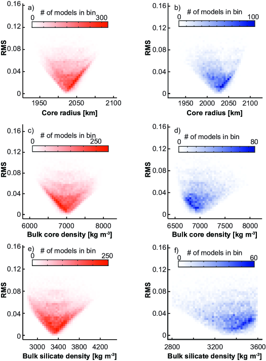
Figure 8: Two-dimensional histograms summarizing N-layer internal structure models of Mercury with Fe–Si core compositions based on the approach of Hauck et al., (2013) and current best estimates of $C/MR^{2}$ and $C_{{\rm m}\mbox{{\tiny+}}{\rm cr}}/C$ (Section 5.2). The left column (a, c, and e) represents models that include a three-layer silicate shell with a crust, mantle, and denser solid layer at the base of the mantle. The right column (b, d, and f) represents models that include a two-layer silicate shell with a crust and mantle. Shown are the recoveries of the radius of the top of the liquid outer core (a and b), bulk density of the metallic core (c and d), and bulk density of the silicate, solid, outermost shell of the planet (e and f). The vertical axes show the goodness of fit expressed as a fractional root mean square difference (Equation 32). Si contents of the metallic core in these models vary from 0 to 17 wt % (Hauck et al.,, 2013).

The bulk densities of the material above and below the transition between the liquid core and outermost shell are also well established across a broad range of assumed core compositions and modeling approaches (e.g., Hauck et al.,, 2013; Rivoldini and Van Hoolst,, 2013). The bulk density of the core material has been found to be distributed in the range 6 750–7 540 ${\rm kg\,m}^{-3}$, with central values falling in the interval 6 900–7 300 ${\rm kg\,m}^{-3}$ and one-standard-deviation uncertainties of less than 5% of the central value (Hauck et al., 2013; Rivoldini and Van Hoolst, 2013). The bulk density of the solid outermost shell of Mercury is distributed in the range 3 020–3 580 ${\rm kg\,m}^{-3}$, with central values falling in the interval 3 200–3 400 ${\rm kg\,m}^{-3}$ and one-standard-deviation uncertainties of approximately 6% of the central value.

One of the more intriguing proposals for the structure of Mercury’s interior is the idea that a solid FeS layer could stably form at the core-mantle boundary. From a chemical standpoint, this layer originates in the core and resides at the top of the core. From a mechanical standpoint, however, a solid layer resides at the bottom of the mantle (Figure 7). The solid FeS layer hypothesis resulted from two observations. First, the chemically reducing conditions observed at the surface, if pertinent to the bulk of the planet, imply that Si will increasingly partition into the core with decreasing oxygen fugacity. At the pressures of Mercury’s core-mantle boundary, Fe–S–Si liquids separate into two liquid phases over a broad range of compositions (Morard and Katsura,, 2010). Hauck et al., (2013) estimated from the FeS (IV) EOS that the solid phase was less dense than the residual liquid and could float rather than sink. Second, the best-fitting models (e.g., those with the lowest RMS values in Figure 8, but not necessarily with the highest histogram values) tend to have bulk densities for the solid outermost shell of Mercury that are larger than $\sim$3 200 ${\rm kg\,m}^{-3}$, the approximate density expected for Fe-poor to Fe-absent mantle minerals such as forsterite and enstatite. For these reasons, Hauck et al., (2013) investigated both the situation with and without an FeS layer. However, the one-standard-deviation uncertainty in the outer shell bulk density is $\sim$200 ${\rm kg\,m}^{-3}$ and permits a wide array of possible density configurations, with and without a solid FeS layer at the top of the core. Furthermore, recent calculations by Knibbe and van Westrenen, (2015) question whether solid FeS is capable of floating at the top of the core, thus potentially preventing a substantial FeS layer from forming at the core-mantle boundary. Additional work on the EOS of solid FeS IV at the appropriate conditions is warranted.

Recently, experiments investigating the partitioning of S and Si between silicate and metallic melts for Mercury-like compositions (Chabot et al.,, 2014) have provided an opportunity to examine more closely the nature of the core-mantle boundary region. Figure 9 illustrates a comparison of the bulk core compositions of the internal structure models of Hauck et al., (2013) containing a possible solid FeS layer at the top of the core with the predicted ranges of core compositions compatible with MESSENGER geochemical observations of the surface (Chabot et al.,, 2014). Also shown are the limits on compositions in the Fe–S–Si system that display liquid-liquid immiscibility at the relevant pressures of 6 and 10 GPa. Compositions to the right of the immiscibility limit curves display immiscibility and are prone to phase separation at the given pressure. While the majority of core compositions in the Fe–S–Si models of Hauck et al., (2013) are consistent with the segregation of Fe–S-rich liquids at the top of Mercury’s core, the general lack of overlap of recent geochemical predictions of possible core compositions with the immiscibility limits (Chabot et al.,, 2014) suggests that liquid-liquid phase separation may not be preferred. The further consequence, of course, is that the conditions for crystallization of an FeS phase at the top of the core appear less likely than the immiscibility limits alone previously suggested. However, as is apparent from Figure 9, the preferred core compositions of Chabot et al., (2014) and the most probable models that match the density and moment of inertia parameters do not generally overlap. There are several possible explanations for the discrepancy. First, it may be that the surface abundance of S cannot yield reliable insights about core composition, either because the surface abundance is not representative of the planet’s bulk silicate composition, or because chemical equilibrium was not satisfied during core formation. Second, it is possible that a modeling approach not investigated so far is required, e.g., a single, miscible Fe–S–Si liquid phase, rather than two fully separated Fe–S and Fe–Si phases. Third, it is possible that the partitioning behavior observed at atmospheric pressure by Chabot et al., (2014) is not representative of core conditions. Indeed, a recent geochemical experimental study with differing silicate compositions and at slightly higher pressures (Namur et al.,, 2016b) suggests that the mantle may contain more S than the surface rocks. In that case, the bulk core S content may be larger and the core conditions may belong to the immiscibility field. However, that conclusion and the thickness of any possible FeS layer depend strongly on Mercury’s bulk S content.

Understanding the existence and size of an inner core on Mercury is a critical goal because an inner core influences several aspects of the planet’s evolution, including magnetic field generation (Chapters 5 and 19), global contraction (Chapters 10 and 19), and rotational state (Section 9). However, the size of the inner core is difficult to quantify, for two reasons. First, the density contrast across the inner-outer core boundary is modest (e.g., Hauck et al.,, 2013; Rivoldini and Van Hoolst,, 2013). Second, the inner core comprises only a small fraction of the mass and density distribution of the planet. Indeed, models with assumptions about the melting relationships of the core can typically place only upper limits on the size of the inner core, and these upper limits are large. In models with core concentrations of S exceeding a few wt %, upper limits are $\sim$1 450 km, i.e., $R_{\rm ic}/R\lesssim 0.6$ (Rivoldini and Van Hoolst,, 2013; Dumberry and Rivoldini,, 2015; Knibbe and van Westrenen,, 2015). Upper limits as high as 1 700–1 800 km can be reached in models with low core concentrations of S (Rivoldini and Van Hoolst,, 2013; Dumberry and Rivoldini,, 2015; Knibbe and van Westrenen,, 2015). Growth of an inner core to that size over the past $\sim$4 billion years is likely incompatible with the inferred amount of global contraction of the planet from measurements of tectonic structures on the surface (Section 9, Chapter 19). Models without an assumed core melting relationship constraint do not place strong limits on the size of the solid inner core, although there is a slight preference for models with an inner core radius less than $\sim$60% of the core radius or $\sim$50% of the planetary radius (Hauck et al.,, 2013). Additional constraints on the size of the inner core are discussed in Section 9.

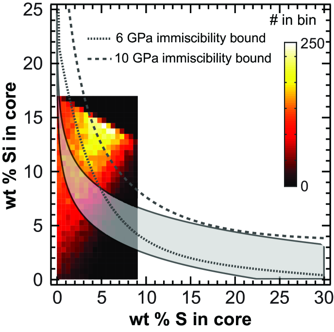
Figure 9: Representation of bulk core S and Si contents in a subset of the internal structure models of Hauck et al., (2013). All models shown have an Fe–S–Si core composition and a solid FeS layer at the base of the mantle, and only models that match the $C/MR^{2}$ and $C_{\rm m+cr}/C$ constraints (Section 5.2) are shown. The two-dimensional histogram indicates the relative number of successful models at each bulk core composition. Immiscibility limits in the Fe–S–Si system at two different pressures are shown by the dotted and dashed lines. Compositions to the right of these lines result in immiscible Fe–S-rich and Fe–Si-rich liquids at the indicated pressure. The gray region illustrates predicted bounds on core composition from metal-silicate partitioning experiments under the assumption that the S content at the surface of Mercury yields reliable constraints on core composition (Chabot et al.,, 2014). The lower and upper boundaries of the gray region represent the expected core compositions for Mercury-like compositions for representative surface S contents of 1 wt % and 4 wt %, respectively.

8 Tidal response

Additional insights about Mercury’s interior structure can be gained by measuring the deformation that the planet experiences as a result of periodic tidal forces. These measurements are informative because the response of a planet to tides is a function of the density, rigidity (i.e., shear modulus), and viscosity of the subsurface materials. Tidal measurements have been used to support the hypothesis of a liquid core inside Venus (Konopliv and Yoder,, 1996) and Mars (Yoder et al.,, 2003), and that of a global liquid ocean inside Titan (Iess et al.,, 2012). In principle, high-precision measurements of the tidal response can be used to rule out models that are otherwise compatible with the density and moment of inertia constraints (Section 7). When a global liquid layer is present, the tidal response is largely controlled by the strength and thickness of the outer solid shell (e.g., Moore and Schubert,, 2000). Because Mercury has a molten outer core (Section 4) and because the thickness of the outer solid shell is known (Sections 5 and 7), tidal measurements enable investigations of the strength of the outer solid shell. This strength depends primarily on the mineralogy and thermal structure of the shell.

8.1 Tidal potential Love number $k_{2}$

The tidal perturbation generated by the Sun on Mercury simultaneously modifies the shape of the planet and the distribution of matter inside the planet. As a result of the redistribution of mass, solar tides also modify Mercury’s gravitational field. From the standard expansion of the gravitational field in spherical harmonics (e.g., Kaula,, 2000), the largest component of the tidal potential is a degree-2 component $\Phi_{2}$ proportional to the mass of the Sun and with a long axis that is aligned with the Sun-Mercury line. The additional potential $\phi_{2t}$ resulting from the deformation of the planet in response to the tidal potential is parameterized by the tidal potential Love number $k_{2}$:

$$\phi_{2t}=k_{2}\>\Phi_{2}.$$ (33)

The tidal component with the largest amplitude has a period $P_{\rm m}=87.9693$ days (Van Hoolst and Jacobs,, 2003), corresponding to Mercury’s orbital period. The Love number $k_{2}$ is a function of $\omega,\rho(r),\mu(r),$ and $\eta(r)$, where $\omega=2\pi/P_{\rm m}$ is the known forcing frequency and $\rho(r)$, $\mu(r)$, and $\eta(r)$ are the density, rigidity, and viscosity profiles. With the appropriate profiles, the Love number $k_{2}$ at the frequency $\omega$ can be calculated by solving the equations of motion inside the planet. These equations consist of three second-order equations that can be transformed into a system of six first-order linear differential equations in radius through a spherical harmonic decomposition in latitude and longitude (Alterman et al.,, 1959). We solve these equations with a slightly modified version of the propagator matrix method (e.g., Sabadini and Vermeersen,, 2004), as described by Wolf, (1994) and by Moore and Schubert, (2000, 2003).

8.2 Rheological models

The rheological response of solid materials is elastic, viscoelastic, or viscous, depending primarily on pressure, temperature, grain size, and timescale of the process under consideration. Other dependencies include melt fraction and water content. Earth’s mantle has a quasi-elastic response on the short timescales associated with seismic waves and a fluid-like response on the long timescales of mantle convection.

The Maxwell rheological model is the simplest model that captures behavior on both short and long timescales. It is completely defined by two parameters, the unrelaxed (i.e., corresponding to an impulsive or infinite-frequency perturbation) rigidity $\mu_{\rm U}$ and the dynamic viscosity $\eta.$ The Maxwell time, defined as

$$\tau_{\rm M}=\frac{\eta}{\mu_{\rm U}},$$ (34)

is a timescale that separates the elastic regime (forcing period $\ll\tau_{\rm M}$) from the fluid regime (forcing period $\gg\tau_{\rm M}$). This simple rheological model is sufficiently accurate to describe the crust of Mercury. The crust is cold and responds elastically ($\tau_{\rm M,crust}=10^{5}$ y). We treat the liquid outer core as an inviscid fluid. We also use the Maxwell model to represent the rheology of the inner core, which, if present, has a negligible effect on the tidal response (Padovan et al.,, 2014). However, the Maxwell model fails to capture the response of the mantle at tidal frequencies (e.g., Efroimsky and Lainey,, 2007; Nimmo et al.,, 2012), because it does not provide a good fit to laboratory and field data in the low-frequency seismological range.

We adopt the Andrade pseudo-period rheological model to estimate the response of Mercury’s mantle to tidal forcing (Jackson et al.,, 2010; Padovan et al.,, 2014). In this model, the ratio of strain to stress, or inverse rigidity, is represented by a complex compliance. The expressions for the real (R) and imaginary (I) parts of the dynamic compliance in the Andrade model are (Jackson et al.,, 2010):

$$J_{\rm R} = J_{\rm U}\left\{1+\beta^{*}\Gamma\left(1+n\right)\omega_{\rm a}^{-n}\cos\left(\frac{n\pi}{2}\right)\right\},$$ (35)

$$J_{\rm I} = J_{\rm U}\left\{\beta^{*}\Gamma\left(1+n\right)\omega_{\rm a}^{-n}\sin\left(\frac{n\pi}{2}\right)+\frac{1}{\omega_{\rm v}\tau_{\rm M}}\right\}.$$ (36)

$J_{\rm U}$ is the unrelaxed compliance, $\Gamma$ is the gamma function, and $n$, $\beta^{*}=\beta/J_{\rm U}$, and $\tau_{\rm M}=\eta J_{\rm U}$ are related to parameters appearing in the Andrade creep function $J(t)=J_{\rm U}+\beta t^{n}+t/\eta.$ The pressure ($P$), temperature ($T$), and grain size ($d$) dependencies are introduced through the pseudo-period master variable $X_{\rm B}=2\pi/\omega_{\rm a,v}$:

$$X_{\rm B} = T_{0}\left(\frac{d}{d_{\rm Ref}}\right)^{-m_{\rm a,v}}$$ (37)

$$\times\exp\left[\left(\frac{-E}{R}\right)\left(\frac{1}{T}-\frac{1}{T_{\rm Ref}}\right)\right]$$

$$\times\exp\left[\left(\frac{-V}{R}\right)\left(\frac{P}{T}-\frac{P_{\rm Ref}}{T_{\rm Ref}}\right)\right],$$

where $T_{0}$ is the period of the applied forcing (in this case the period of the primary tidal component), $m_{\rm a}$ ($m_{\rm v}$) is the grain size exponent for anelastic (viscous) processes, and $R$ is the gas constant. $P_{\rm Ref}$, $T_{\rm Ref}$, and $d_{\rm Ref}$ indicate reference values (Table 1). The unrelaxed shear modulus $\mu_{\rm U}=1/J_{\rm U}$ is itself dependent on pressure and temperature, which we characterize by a simple Taylor expansion truncated at linear terms: $\mu_{\rm U}\left(P,T\right)=\mu_{\rm U}^{\rm Ref}+(\partial\mu/\partial P)(P-P_{\rm Ref})+(\partial\mu/\partial T)(T-T_{\rm Ref})$. The frequency-dependent shear modulus $\mu(\omega)$, quality factor $Q(\omega)$, and viscosity $\eta(\omega)$ are all obtained from the dynamic compliance, as follows (Jackson et al.,, 2010; Padovan et al.,, 2014):

$$\mu\left(\omega\right) = \left[J^{2}_{\rm R}\left(\omega\right)+J^{2}_{\rm I}\left(\omega\right)\right]^{-1/2},$$ (38)

$$Q\left(\omega\right) = \frac{J_{\rm R}\left(\omega\right)}{J_{\rm I}\left(\omega\right)},$$ (39)

$$\eta\left(\omega\right) = \frac{1}{\omega_{0}J_{\rm I}\left(\omega\right)},$$ (40)

where $\omega_{0}=2\pi/T_{0}.$ Our choice of model parameters is described in Table 1 and Section 8.3.

Table 1: Rheological models for the interior of Mercury.

Layer	Model	Parameter	Definition	Value
Crust	Maxwell
		$\mu_{\rm U}$	Unrelaxed rigidity	55 GPa
		$\eta$	Dynamic viscosity	$10^{23}$ Pa s
Mantle	Andradea
		$\mu_{\rm U}^{\rm Ref}$	Unrelaxed rigidityb	$59-71$ GPa
		$T_{\rm b}$	Mantle basal temperaturec	$1\,600-1\,850$ K
		$n$	Andrade creep coefficient	0.3
		$\beta^{*}$	Andrade creep parameter	0.02
		$P_{\rm Ref}$	Reference pressure	0.2 GPa
		$T_{\rm Ref}$	Reference temperature	1 173 K
		$d_{\rm Ref}$	Reference grain-size	$3.1$ $\mu{\rm m}$
		$d$	Grain size	$1\,{\rm mm}-1\,{\rm cm}$
		$m_{\rm a},$ $m_{\rm v}$	Grain size exponents	$1.31,$ $3$
		$V$	Activation volume	$10^{-5}$ m3mol-1
		$E_{\rm B}$	Activation energy	$303\times 10^{3}$ kJ mol-1
FeS	Andraded
Outer core	Inviscid fluid
		$\mu_{\rm U}$	Unrelaxed rigidity	0 Gpa
		$\eta$	Dynamic viscosity	0 Pa s
Inner core	Maxwell
		$\mu_{\rm U}$	Unrelaxed rigidity	$100$ GPa
		$\eta$	Dynamic viscosity	$10^{20}$ Pa s

Our choices of Andrade model parameter values (Table 1) are based on data obtained at periods smaller than $10^{3}$ s (Jackson et al.,, 2010), whereas the main tide of Mercury has a period $>10^{6}$ s. The extrapolation to long time scales can be validated to some extent by two considerations. First, we verified that equation (40) yields viscosity values at long timescales ($>10$ My) that fall within the interval for convective viscosities commonly assumed in terrestrial mantle convection simulations ($10^{20}-10^{23}$ Pa s). Second, we verified that, at timescales appropriate for glacial rebound on Earth ($\sim$10⁴ y), the predicted viscosity values ($10^{20}-10^{21}$ Pa s) compare favorably with those inferred from geodynamical data (e.g., Kaufmann and Lambeck,, 2000).

The choice of Andrade model parameter values (Table 1) is also based on laboratory data for olivine (Jackson et al.,, 2010), whereas we apply the model to a variety of mineralogies (Table 2). This extrapolation to other mineralogies is not strictly correct, especially for mantle models in which olivine is not the dominant phase. However, the Andrade model has been successfully applied to the description of dissipation in rocks, ices, and metals (e.g., Efroimsky,, 2012; and references therein). The broad applicability of the model over a wide range of physical and chemical properties suggests that the model can provide an adequate description of the rheology of silicate minerals.

Recent results of laboratory experiments and thermodynamic simulations based on Mercury surface compositions (Vander Kaaden and McCubbin,, 2016; Namur et al.,, 2016a) suggest an olivine-rich source for both the northern smooth plains and the high-Mg region of the intercrater plains and heavily cratered terrain. These results are in accord with an olivine-dominated mineralogy for the mantle of Mercury and further support our model parameter choices.

8.3 Methods

We restrict our analysis to interior models that are compatible with the observed bulk density $\rho$, moment of inertia $C,$ and moment of inertia of the solid outer shell $C_{{\rm m}\mbox{{\tiny+}}{\rm cr}}$. By design, the subset of interior models has distributions of $\rho$, $C,$ and $C_{{\rm m}\mbox{{\tiny+}}{\rm cr}}$ that are approximately Gaussian with means and standard deviations that match the nominal values of the observables and their one-standard-deviation errors. The mean density $\rho$ has a Gaussian distribution with mean and standard deviation equal to 5430 ${\rm kg\,m}^{-3}$ and 10 ${\rm kg\,m}^{-3}$, respectively. For $C$ and $C_{{\rm m}\mbox{{\tiny+}}{\rm cr}}$, we choose Gaussian distributions with means and standard deviations defined by the observed values and errors (Section 5.2).

We treat the interior of Mercury as a series of spherically symmetric, incompressible layers characterized by density, thickness, rigidity, and viscosity. We start with the density profiles calculated by Hauck et al., (2013), but we replace the $\sim$1000 layers that characterize the core in these models with two homogeneous layers representing the solid inner core and the liquid outer core. This simplification is warranted because the tidal response is dominated by the presence of a liquid outer core and is largely independent of the detailed density structure of the core. It reduces the computational cost by about three orders of magnitude and introduces only a small ($<$2%) error in the estimated value of $k_{2}$. This error is smaller than the variations induced by the unknown mineralogy and thermal state of the mantle (Padovan et al.,, 2014).

For the core of Mercury, we focus on the Si-bearing subset of models analyzed by Hauck et al., (2013), because this subset is most consistent with the chemically reducing conditions inferred from surface materials (Section 6). We also consider the subset of models with a solid FeS V layer included at the base of the mantle (Hauck et al., (2013) and Section 7). For the silicate mantle of Mercury, we consider six mineralogical models based on the works of Rivoldini et al., (2009) and Malavergne et al., (2010) (Table 2).

Table 2: Mineralogical models for the mantle of Mercury.

Model	Grt	Opx	Cpx	Qtz	Spl	Pl	Mw	Ol	$\mu_{\rm U}^{\rm Ref}\>(\rm{GPa})$
CB	–	66	4	22	4	4	–	–	59
EH	–	78	2	8	–	12	–	–	65
MA	23	32	15	–	–	–	–	30	69
TS	25	–	–	–	8	–	2	65	71
MC	15	50	9	–	–	–	–	26	68
EC	1	75	7	17	–	–	–	–	60

Our use of the Andrade model (Section 8.2) for the rheological properties of the mantle requires knowledge of the radial profiles of unrelaxed rigidity $\mu_{\rm U}$, temperature $T,$ and pressure $P$ in the outer solid shell. For each of the six mineralogical models, we compute a composite rigidity $\mu_{\rm U}^{\rm Ref}$ (Table 2) with Hill’s expression (Watt et al.,, 1976) at $T=T_{\rm Ref}$ and $P=P_{\rm Ref}$. The pressure profile in the outer solid shell is obtained by evaluating the overburden pressure as a function of depth. The temperature in the mantle is computed by solving the static heat conduction equation with heat sources in spherical coordinates (e.g., Turcotte and Schubert,, 2002) in the mantle and crust. For the crust, we adopted the surface value of the heat production rate $H_{0}=2.2\times 10^{-11}\>\rm{W\;kg^{-1}}$ (Peplowski et al.,, 2012). For the mantle, we used a value of $H_{0}/2.5,$ which is compatible with the enrichment factor derived by Tosi et al., (2013). Temperature profiles are fairly insensitive to the value of the thermal conductivity: we used a value $k_{m}=3.3\,{\rm Wm}^{-1}{\rm}K^{-1}$ but confirmed that a value of $k_{m}=5\,{\rm Wm}^{-1}{\rm}K^{-1}$ yields essentially the same results. We establish two boundary conditions: the temperature at the surface of Mercury $T_{\rm S}$ and the temperature at the base of the mantle $T_{\rm b}$. The latter provides the primary control on the temperature profile. $T_{\rm S}$ is set to $440$ K, a value obtained with an equilibrium temperature calculation. Both Rivoldini and Van Hoolst, (2013) and Tosi et al., (2013) indicate $T_{\rm b}$ values in the range 1 600–1 900 K. We define two end-member profiles: a cold-mantle profile with $T_{\rm b}=1\,600$ K and a hot-mantle profile with $T_{\rm b}=\,1\,850$ K. A larger value of $T_{\rm b}$ (e.g., 1 900 K) would result in partial melting at the base of the mantle according to the peridotite solidus computed by Hirschmann, (2000). We did not consider the presence of partial melting.

There is a scarcity of laboratory data for FeS V, which is the phase relevant at the pressure and temperature conditions at the bottom of the mantle of Mercury (Fei et al.,, 1995). We consider the effects of the FeS layer only in the cold-mantle case ($T_{\rm b}=1\,600$ K), because at higher temperatures the FeS would be liquid (see the phase diagram given by Fei et al.,, 1995). We model the rheological response of this layer by assuming that it has the same rheological properties as those at the base of the mantle. This assumption results in a lower bound on the $k_{2}$ estimates because we expect the viscosity of this layer to be lower than that of the silicate layer. The viscosity scales as the exponential of the inverse of the homologous temperature (i.e., the ratio of the temperature of the material to the solidus temperature) (e.g., Borch and Green,, 1987). At $T=1\,600$ K, the homologous temperature of the FeS V is larger than that of the silicates. In addition, the unrelaxed rigidity of FeS V is likely to be smaller than that for mantle material because the rigidity of troilite (or FeS I, the phase at standard pressure and temperature) is 31.5 GPa (Hofmeister and Mao,, 2003).

We apply our calculations to five different models (nominal, cold and stiff, hot and weak, FeS-layer, and 1-mm grain size). Given the 1 600–1 850 K range for the basal mantle temperature and 59–71 GPa range for the unrelaxed rigidity of the mantle, we define a nominal model with $T_{\rm b}=1\,725$ K and $\mu_{\rm U}=65$ GPa. Changes in basal mantle temperature and unrelaxed rigidity have similar but opposite effects on the tidal response. Accordingly, we define two end-member models: a cold and stiff mantle model with $T_{\rm b}=1\,600$ K and $\mu_{\rm U}=71$ GPa and a hot and weak mantle model with $T_{\rm b}=1\,850$ K and $\mu_{\rm U}=59$ GPa. Our fourth model is a cold mantle model ($T_{\rm b}=1\,600$ K) with nominal rigidity ($\mu_{\rm U}=65$ GPa) and an FeS layer at the bottom of the mantle. In all of these four models, we use a nominal grain size $d=1$ cm, a value compatible with the estimated grain size in the mantles of the Moon and Mars (Nimmo et al.,, 2012; Nimmo and Faul,, 2013). Our fifth and last model is a variation of the nominal model in which we consider a grain size of $d=1$ mm. Model parameters are summarized in Table 3.

Table 3: Characteristics of five mantle models for the estimation of Mercury’s tidal response.

Model	$\mu_{\rm U}$, GPa	$T_{\rm b}$, K	$d$, mm	${\rm FeS}?$
Nominal	65	1 725	10	no
Cold and stiff	71	1 600	10	no
Hot and weak	59	1 850	10	no
FeS layer	65	1 600	10	yes
1-mm grain size	65	1 725	1	no

Our procedure for evaluating the Love number $k_{2}$ and corresponding uncertainties is as follows. For each of the five cases described in Table 3, we use approximately $6\times 10^{4}$ density profiles from the previously identified subsets of models from Hauck et al., (2013). For each profile, we construct an interior model and calculate the value of $k_{2}$. We then fit a Gaussian distribution to the $\sim$6$\times 10^{4}$ calculated $k_{2}$ values, as was done by Padovan et al., (2014). We report the Love number and associated error as the mean and standard deviation of the Gaussian fit. Our values differ somewhat from those of Padovan et al., (2014) because we incorporated the most recent estimates of the moments of inertia in this work (Equations 19 and 20).

8.4 Results

Our Love number calculations for models with a molten outer core yield values $k_{2}\simeq 0.5$. However, for models with a completely solid core, we found $k_{2}$ values that are approximately an order of magnitude smaller. Measurements of Mercury’s tidal response (Section 3.4) therefore confirm the presence of a molten outer core.

Our results also show that the tidal response is enhanced by higher mantle basal temperatures and by lower mantle rigidities (Figure 10).

The comparison of our calculated values with the $k_{2}$ value measured by Mazarico et al., (2014) indicates that the observed tidal signal is more compatible with cold, rigid mantle models (Figure 10). The $k_{2}$ value measured by Verma and Margot, (2016) admits a wider range of models but still favors models with a cold and stiff mantle or a subset of the FeS-layer models. It is likely that models with an FeS layer at the bottom of the mantle and high mantle rigidity ($\mu_{\rm U}=71$ GPa) would also be compatible with $k_{2}$ measurements, but there are questions about the plausibility of such a layer (Knibbe and van Westrenen,, 2015; Section 7.4).

The conclusion drawn from the modeling of the tidal Love number seems robust with respect to details of the thermal model. For instance, consideration of a surficial regolith layer with low thermal conductivity increases the temperature in the interior, which results in larger $k_{2}$ model values and further favors a cold and stiff mantle. Consideration of a higher solidus temperature and $T_{\rm b}>1\,850$ K would also strengthen the conclusion that Mercury’s mantle is likely cold and stiff. Unfortunately, the robustness of the conclusion is undermined because of the large standard deviations associated with the modeled $k_{2}$ values and because the actual $k_{2}$ value may extend beyond the range given by the one-standard-deviation uncertainties. The overlap in simulated $k_{2}$ values for the five mantle models implies that even a more precise $k_{2}$ measurement would not be sufficient to identify a unique model at this time. However, a reduction in uncertainties of both the measured Love number and moments of inertia will narrow the range of mantle models that are compatible with observations.

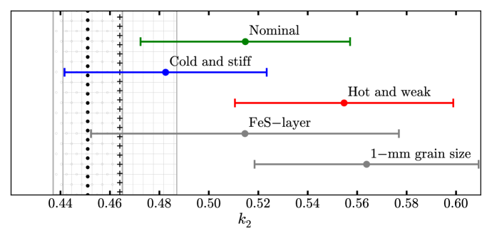
Figure 10: Calculated values of the tidal Love number $k_{2}$ for five models constructed under different assumptions about the rheological properties and physical structure of the outer solid shell of Mercury (Table 3). The vertical lines and hatch patterns represent two independent determinations of $k_{2}$ and associated one-standard-deviation uncertainties measured by radio tracking of the MESSENGER spacecraft. Dot symbols correspond to the results of Mazarico et al., (2014), and plus symbols correspond to the results Verma and Margot, (2016).

9 Influence of solid inner core

Torques between layers in Mercury’s interior can influence the spin state. Peale et al., (2014) derived the behavior of Mercury’s spin axis orientation under the influence of a variety of core-mantle torques, including gravitational, tidal, magnetic, topographic, viscous, and pressure torques. They showed that tidal torques are small in comparison to magnetic and topographic torques, which are themselves small compared with viscous torques. These dissipative torques would drive the mantle spin away from the Cassini state if it were not for the action of a pressure torque between the outer core and the mantle. The pressure torque is due to fluid pressure at the core-mantle boundary, which is not spherically symmetric because of its hydrostatic, approximately ellipsoidal shape. In the absence of an inner core, the pressure torque dominates the spin axis evolution and drives the mantle spin close to the Cassini state position.

Peale et al., (2016) considered the additional torques due to an inner core. Their theoretical formalism is general and applicable to other planets, including Earth. The shape of the inner core is distorted by the non-radial gravitational field, and a gravitational torque between inner core and mantle develops. The relationship between the observed obliquity and the moment of inertia (Equation 5), which is based on solar torques, must be modified to account for this additional torque. If the inner core is small ($R_{\rm ic}/R<0.35$), the mantle spin follows the Cassini state orientation sufficiently closely that the moment of inertia determination is not compromised. However, if the inner core size exceeds 35% of the planetary radius, the additional torque would drag the mantle spin away from the Cassini state by an amount that exceeds the current observational uncertainty of 5 arcseconds, and the polar moment of inertia would have to be re-evaluated. In the presence of an inner core, the obliquity of the mantle spin axis corresponds to a smaller polar moment of inertia than that inferred from the situation with no inner core. This change in the value of the moment of inertia can be evaluated for a variety of interior models by tracking the evolution of the spin under the action of all relevant torques and enforcing the requirement that the mantle spin axis orientation remains within the uncertainty region of the radar observations. Peale et al., (2016) performed this calculation for a variety of inner core sizes and inner core densities. They found that the required adjustment to the value of the moment of inertia increases with both inner core density and inner core size. For an inner core density of $9\,300{\ \rm kg\,m}^{-3}$, they found corrected values of $C/MR^{2}=0.346,0.343,0.330,0.327,{\rm and}0.323$ for inner core sizes of $R_{\rm ic}/R=0.0,0.3,0.4,0.5,{\rm and}0.6$, respectively (Peale et al.,, 2016). Because 85% of the best-fit interior models (Section 10) have inner core densities below $9\,300{\ \rm kg\,m}^{-3}$, the corrections identified by Peale et al., (2016) likely represent upper bounds on any necessary adjustment to the moment of inertia due to the presence of an inner core.

Because of the possible impact of an inner core on the determination of Mercury’s moment of inertia (Dumberry et al.,, 2013; Peale et al.,, 2016), it is important to place bounds on the size of the inner core. We review six lines of evidence. (1) Peale et al., (2016) found that in models with inner cores larger than $R_{\rm ic}/R=0.3$, the inferred mantle densities were only $\sim$3 000${\ \rm kg\,m}^{-3}$. Such low mantle densities are difficult to explain because they are lower than those of materials that likely dominate Mercury’s Fe-poor interior, such as Mg-rich olivine and Mg-rich orthopyroxene, which have densities of $3\,200-3\,300{\ \rm kg\,m}^{-3}$. If the density information is a reliable indicator, the calculations of Peale et al., (2016) suggest an inner core size $R_{\rm ic}/R\leq 0.3$. (2) A similar conclusion can be reached by examining the distribution of internal structure models. We find that 65% of models that provide the best fit to existing observations (Section 10) have a small inner core ($R_{\rm ic}/R<0.35$). (3) Independent constraints on inner core size arise from the fact that planetary contraction is due in part to inner core solidification. The observed planetary contraction of 7 km (Byrne et al.,, 2014; Chapter 10) suggests that the inner core size does not exceed 800–1 000 km, i.e., $R_{\rm ic}/R\lesssim 0.4$,  (Grott et al.,, 2011; Dumberry and Rivoldini,, 2015). Knibbe and van Westrenen, (2015) found upper bounds as large as $R_{\rm ic}/R\lesssim 0.7$ for certain values of model parameters, but they did not consider the effects of mantle contraction, which may amount for about half of the planetary contraction (Tosi et al.,, 2013). (4) Simulations of Mercury’s magnetic field provide another indicator about the size of the inner core. Dynamo models that can reproduce the observed features of Mercury’s magnetic field (Cao et al.,, 2014) favor small inner cores ($R_{\rm ic}/R_{\rm oc}<0.5$, i.e., $R_{\rm ic}/R<0.4$). (5) Dumberry and Rivoldini, (2015) further argued that, in some situations, the dynamics of snow formation in the fluid core would place an upper limit on the inner core radius of 650 km ($R_{\rm ic}/R<0.27$). (6) Finally, several authors have noted that a large inner core $(R_{\rm ic}/R>0.4)$ would produce detectable signatures in the librations of the planet (Veasey and Dumberry,, 2011; Dumberry,, 2011; Van Hoolst et al.,, 2012), but such signatures have not been detected to date. There is considerable interest in improving measurements of the longitudinal librations in an attempt to place bounds on the size of Mercury’s inner core (Veasey and Dumberry,, 2011; Dumberry,, 2011; Van Hoolst et al.,, 2012), although it is not clear that the precision of the current measurement techniques would enable a detection of the inner core signature.

To summarize, there is some circumstantial evidence that Mercury’s inner core is small ($R_{\rm ic}/R\lesssim 0.35$) and that the existing estimate of $C/MR^{2}=0.346\pm 0.009$ remains valid. However, no direct measurements of the inner core size exist, which reduces our confidence in the knowledge of Mercury’s moment of inertia. Improved measurements of the librations or direct measurements of the inner core size will be required to eliminate the uncertainty. One approach would be to deploy seismometers on the surface and measure seismic signals triggered by tides, internal activity, explosive charges, or impacts.

10 Representative model

The observational evidence from spin, tidal, and compositional observations, summarized in Table 4, favors a Mercury interior model with a core composition dominated by Fe-Si and with a small or no solid FeS layer. Therefore, models in which the core is treated as an Fe-Si end-member are likely representative of Mercury’s interior.

Table 4: Summary of observational constraints used for the calculation of internal structure models.

Parameter	Symbol	Value	Uncertainty	Unit
Mass	$M$	3.301110	0.00015	$10^{23}$ kg
Radius	$R$	2 439.36	0.02	km
Density	$\rho$	5 429.30	0.28	${\rm kg\,m}^{-3}$
Gravity spherical harmonic	$C_{20}$	-5.0323	0.0022	$10^{-5}$
Gravity spherical harmonic	$C_{22}$	0.8039	0.0006	$10^{-5}$
Tidal Love number	$k_{2}$	0.455	0.012
Obliquity	$\theta$	2.036	0.058	arcminutes
Amplitude of longitude librations	$\phi_{0}$	38.7	1.0	arcseconds
Moment of inertia factor	$C/MR^{2}$	0.346	0.009
Moment of inertia of mantle and crust	$C_{{\rm m}\mbox{{\tiny+}}{\rm cr}}/{C}$	0.425	0.016
Crustal thickness	$h_{\rm cr}$	35–53		km
Crustal density	$\rho_{\rm cr}$	2 700–3 100		${\rm kg\,m}^{-3}$

Our preferred models include bounds on crustal thickness and density. Analyses of gravity-to-topography ratios suggest an average crustal thickness of $35\pm 18$ km (Padovan et al.,, 2015) and $>38$ km (James et al.,, 2015). We combine these bounds into a preferred crustal thickness in the range 35–53 km (Table 4). The grain density of crustal material can be determined from a normative mineralogy, which itself is guided by observations of elemental abundances at the surface of Mercury (Weider et al.,, 2014). With this approach, Padovan et al., (2015) obtained grain densities of 3 014 ${\rm kg\,m}^{-3}$ and 3 082 ${\rm kg\,m}^{-3}$ for the northern smooth plains and for heavily cratered terrain and intercrater plains, respectively. If we take into account porosity values of up to 12% as observed on the Moon (Wieczorek et al.,, 2013), our preferred crustal densities are in the range 2 700–3 100 ${\rm kg\,m}^{-3}$ (Table 4).

We updated the analysis of Hauck et al., (2013) to conform to the radius and density values listed in Table 4. In addition, we specified an initial crustal thickness in the range 0–70 km, a crustal density in the range 2 700–3 100 ${\rm kg\,m}^{-3}$, and a core Si content in the range 0–17 wt %. This analysis yielded 1 016 236 Fe-Si interior models with considerable scatter in structural properties. From these models, one can extract a random sample of models for which the distributions of ${C}/{MR^{2}}$ and ${C_{{\rm m}\mbox{{\tiny+}}{\rm cr}}}/{C}$ values match the observed values and corresponding one-standard-deviation uncertainties (Table 4). We further restricted the set of preferred models to those that provide the closest agreement to the observed values of ${C}/{MR^{2}}$ and ${C_{{\rm m}\mbox{{\tiny+}}{\rm cr}}}/{C}$. All 1 479 models in this subset have RMS $<$ 0.005, where the RMS metric is described by equation (32). These 1 479 best-fit models constitute a family of representative models that can be used to illustrate the remaining scatter in the values of Mercury’s internal structure parameters (Table 5). Among the subset of models that provide the closest match to observational data, the radius of Mercury’s core, $R_{\rm oc}=2024\pm 9$ km, is determined with $<$0.5% precision and represents 83% of the radius of the planet.

Table 5: Statistical properties of interior structure model parameters and corresponding PRMM values.

Parameter	minimum	1st quartile	median	3rd quartile	maximum	mean	std. dev.	PRMM
${C}/{MR^{2}}$	0.34430	0.34523	0.34596	0.34670	0.34771	0.34597	0.00089	0.34573
${C_{{\rm m}\mbox{{\tiny+}}{\rm cr}}}/{C}$	0.42294	0.42418	0.42496	0.42578	0.42712	0.42497	0.00102	0.42482
$R_{\rm ic}$	0.01877	310.780	623.280	1003.60	1790.82	666.577	420	369.433
$R_{\rm oc}$	2009.31	2016.69	2021.30	2029.62	2062.56	2023.66	9.09	2015.48
$R_{\rm m}$	2369.37	2385.60	2401.37	2419.32	2439.35	2402.61	19.9	2401.20
$\rho_{\rm ic}$	7368.25	8295.31	8659.58	8991.33	10214.90	8652.52	488	8215.62
$\rho_{\rm oc}$	5937.29	6775.76	7010.49	7087.14	7187.97	6909.98	237	7109.73
$\rho_{\rm m}$	3206.19	3288.90	3333.75	3388.10	3593.18	3343.35	71.8	3278.98
$\rho_{\rm cr}$	2700.28	2807.00	2898.57	3006.28	3099.78	2903.03	116	2979.19
$\rho_{{\rm ic}\mbox{{\tiny+}}{\rm oc}}$	6671.42	6976.74	7053.32	7102.67	7190.40	7034.32	88.3	7116.54
$\rho_{{\rm m}\mbox{{\tiny+}}{\rm cr}}$	3198.01	3255.43	3286.49	3327.32	3531.21	3295.84	53.0	3247.21
$\rho$	5428.34	5429.11	5429.30	5429.52	5430.53	5429.32	0.31	5429.66
$M_{\rm ic}$	2.588$\times 10^{08}$	1.101$\times 10^{21}$	8.962$\times 10^{21}$	3.582$\times 10^{22}$	1.773$\times 10^{23}$	2.288$\times 10^{22}$	2.95$\times 10^{22}$	1.735$\times 10^{21}$
$M_{\rm oc}$	6.728$\times 10^{22}$	2.084$\times 10^{23}$	2.351$\times 10^{23}$	2.428$\times 10^{23}$	2.446$\times 10^{23}$	2.213$\times 10^{23}$	2.93$\times 10^{22}$	2.423$\times 10^{23}$
$M_{\rm m}$	6.964$\times 10^{22}$	7.464$\times 10^{22}$	7.789$\times 10^{22}$	8.152$\times 10^{22}$	8.631$\times 10^{22}$	7.813$\times 10^{22}$	4.15$\times 10^{21}$	7.771$\times 10^{22}$
$M_{\rm cr}$	1.998$\times 10^{18}$	4.319$\times 10^{21}$	8.020$\times 10^{21}$	1.147$\times 10^{22}$	1.567$\times 10^{22}$	7.822$\times 10^{21}$	4.21$\times 10^{21}$	8.368$\times 10^{21}$
$M_{{\rm ic}\mbox{{\tiny+}}{\rm oc}}$	2.432$\times 10^{23}$	2.439$\times 10^{23}$	2.441$\times 10^{23}$	2.444$\times 10^{23}$	2.454$\times 10^{23}$	2.442$\times 10^{23}$	3.95$\times 10^{20}$	2.441$\times 10^{23}$
$M_{{\rm m}\mbox{{\tiny+}}{\rm cr}}$	8.484$\times 10^{22}$	8.583$\times 10^{22}$	8.611$\times 10^{22}$	8.639$\times 10^{22}$	8.702$\times 10^{22}$	8.609$\times 10^{22}$	3.92$\times 10^{20}$	8.622$\times 10^{22}$
$M$	3.301$\times 10^{23}$	3.301$\times 10^{23}$	3.301$\times 10^{23}$	3.301$\times 10^{23}$	3.302$\times 10^{23}$	3.301$\times 10^{23}$	1.93$\times 10^{19}$	3.301$\times 10^{23}$

We describe an example among the 1 479 models in some detail (Table 5 and Fig. 11). This model is representative in the sense that its structural properties match Mercury’s mass, radius, and moments of inertia, as well as our preferred bounds on crustal thickness and density. However, we emphasize that Mercury’s inner core properties are unknown. The inner core properties of the chosen model are therefore illustrative and not representative. We also emphasize that our chosen model is no better than any other model that fits the observational data. The model does have desirable structural properties, and, as such, it may be useful for a variety of modeling tasks. We refer to this model as the Preliminary Reference Mercury Model (PRMM).

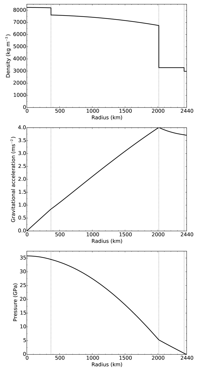
Figure 11: Illustration of the density, gravitational acceleration, and pressure corresponding to a model of Mercury’s interior that closely matches the mass, radius, and moments of inertia of Mercury (PRMM). This model also matches our preferred bounds on crustal thickness and density (Table 4). This model incorporates an Fe-Si core composition and no solid FeS layer. Inner core properties are merely illustrative and not representative. Vertical dotted lines indicate transitions with increasing radius between inner and outer core, core and mantle, and mantle and crust.

In PRMM, Mercury’s mass is divided among inner core (0.5%), outer core (73.4%), mantle (23.5%), and crust (2.5%). The central pressure is 35.77 GPa, and the pressure at the core-mantle boundary is 5.29 GPa. Table 6 lists the parameters that we used to construct PRMM.

Table 6: Parameters used to construct PRMM.

Parameter	Symbol	Value	Units
Mass fraction of Si (below $R_{\rm oc}$)	$\chi$Si	12.83	wt %
Liquid Fe reference density	$\rho_{0,{\rm Fe,1}}$	6471.29	${\rm kg\,m}^{-3}$
Liquid Fe coefficient of thermal expansion	$\alpha_{0,{\rm Fe,1}}$	$9.2\times 10^{-5}$	${\rm K}^{-1}$
Liquid Fe bulk modulus	$K_{0,{\rm Fe,1}}$	115.47	GPa
Liquid Fe pressure derivative of bulk modulus	$K^{\prime}_{0,{\rm Fe,1}}$	4.93
Solid $\gamma$ Fe reference density	$\rho_{0,{\rm Fe,s}}$	7381.34	${\rm kg\,m}^{-3}$
Solid $\gamma$ Fe coefficient of thermal expansion	$\alpha_{0,{\rm Fe,s}}$	$6.4\times 10^{-5}$	${\rm K}^{-1}$
Solid $\gamma$ Fe bulk modulus	$K_{0,{\rm Fe,s}}$	190.73	GPa
Solid $\gamma$ Fe pressure derivative of bulk modulus	$K^{\prime}_{0,{\rm Fe,s}}$	5.62

PRMM was constructed with the benefit of Earth-based and MESSENGER observations that were not available in earlier modeling efforts. Salient differences between PRMM and pre-MESSENGER models include narrower ranges of admissible structural parameter values compared with the ranges considered by Harder and Schubert, (2001), Van Hoolst and Jacobs, (2003), and Riner et al., (2008) and a core size that is substantially larger than the core sizes assumed by Siegfried and Solomon, (1974; 1 660–1 900 km), Stevenson et al., (1983; 1 840–1 900 km), Spohn et al., (2001; $1\,860\pm 80$ km), and Breuer et al., (2007; 1 900 km).

11 Implications

11.1 Thermal evolution

An accurate understanding of Mercury’s thermal evolution requires knowledge of the internal structure, because interior properties dictate the processes and boundary conditions that have governed the evolution. The $\sim$400 km thickness of the silicate mantle and crust has wide-ranging implications. The thickness of this layer is a fundamental control on both the vigor and ultimately the longevity of mantle convection (e.g., Michel et al.,, 2013; Tosi et al.,, 2013; Chapter 19). The vigor of the convection is described by the Rayleigh number, which is the ratio of buoyancy forces to viscous forces in a fluid and scales as the cube of the thickness the layer (e.g., Schubert et al.,, 2001). Pre-MESSENGER models typically invoked a mantle thickness of $\sim$600 km and therefore over-estimated the vigor of the convection by a factor of a few. The MESSENGER-derived value enables more accurate calculations. In particular, the thin mantle implies that convection in Mercury’s mantle has been less vigorous than previously thought and may have completely ceased if the Rayleigh number fell below the critical value for convection. A detailed analysis of Mercury’s thermal evolution is given in Chapter 19.

11.2 Surface geology

Volcanism is intimately tied to mantle convection because decompression melting is the primary source of magma in terrestrial planets. Mercury’s crust, which is the product of perhaps the most efficient crustal extraction among the inner planets (James et al.,, 2015; Padovan et al.,, 2015), was dominantly generated early in the planet’s history when radiogenic heat production was higher (Chapter 19). Mercury’s thin mantle limits the amount of heat transfer because of the reduced vigor of convection and a possible transition to conduction (Section 11.1). The reduced heat transfer lowers the amount of volcanism, cooling, and ensuing global contraction, all of which affect the geological evolution of the surface. In particular, the reduced heat transfer hypothesis is consistent with observations of limited volcanism in the past $\sim$3.5 billion years and an amount of radial contraction accommodated by thrust faulting of no more than 7 km (Byrne et al.,, 2014; Chapters 10 and 19). Tectonic patterns observed at the surface may be due to the interplay of tidal despinning and global contraction (Chapter 10). Surface composition is also affected by mantle thickness, because the horizontal scale of convection cells is similar to the thickness of the convecting layer. Investigations of the source regions of surface volcanic material indicate at least two separate sources (Charlier et al.,, 2013), consistent with limited mixing of the mantle due to the small horizontal scales and limited vigor of convection (Chapter 19).

11.3 Capture in 3:2 resonance

Mercury’s distinctive 3:2 spin-orbit resonance was established at least in part because of Mercury’s internal structure. The structure of the interior and the nature of the interactions among inner core, outer core, and mantle have a profound influence on the evolution of the spin state and the response of the planet to external forces and torques. These processes dictate the overall tectonic and insolation regimes that, in turn, have wide-ranging implications for a variety of questions related to Mercury’s shape, surface geology, thermal regime, and even the presence of polar ice deposits.

The history of Mercury’s spin-orbit configurations has been markedly affected by the presence of a liquid core. It has been suggested that increased energy dissipation at a core-mantle interface would have led to near-certain capture in specific spin-orbit resonances (Goldreich and Peale,, 1967; Counselman and Shapiro,, 1970; Peale,, 1988), although some models indicate 100% capture probability in the 2:1 resonance (Peale and Boss,, 1977), which would prevent evolution to the current configuration. A solution to this problem was found by Correia and Laskar, (2004), who showed that chaotic variations in orbital eccentricity destabilize most spin-orbit resonances and ultimately lead to a 55% capture probability in the 3:2 resonance. After spin state observations revealed Mercury’s liquid core, Correia and Laskar, (2009) added core-mantle friction to their model. They found capture probabilities of 32% (2:1), 26% (3:2), and 22% (5:2). While capture in the 3:2 spin-orbit configuration is not the most probable, the specific outcome depends on the particular realization of orbital eccentricity evolution that Mercury experienced. The capture probability can be increased either if Mercury’s eccentricity reached very low values (Correia and Laskar,, 2009) or if Mercury started in a retrograde spin configuration and became locked in a synchronous state that was later destabilized by large impacts (Wieczorek et al.,, 2012). Core-mantle friction also affects Mercury’s obliquity evolution, which itself can affect resonance capture probabilities (Correia and Laskar,, 2010).

The capture probability results depend on the choice of the tidal torque formulation, which often relies on assumptions of constant time lag or constant phase lag. Models that incorporate a different formulation based on a Darwin-Kaula expansion of the tidal torque yield different capture probabilities (Makarov,, 2012; Noyelles et al.,, 2014) from models that rely on a formulation with constant time lag or constant phase lag. The model of Makarov, (2012) predicts 100% capture probability in the 3:2 resonance but does not include orbital eccentricity variations. The model of Noyelles et al., (2014) predicts capture in a 2:1 or higher resonance unless Mercury was captured in the 3:2 resonance early in its evolution, i.e., before differentiation was complete. However, Correia and Laskar, (2012) argued that large collisions destabilized all spin-orbit resonances experienced early in Mercury’s history and that orbital eccentricity evolution dictated the final outcome. According to Correia and Laskar, (2012), the most probable outcome ($\sim$50%) is capture in the 3:2 resonance, regardless of the details of the tidal formulation, core-mantle friction formulation, or collisional history.

Estimates for the timing of capture in the 3:2 resonance range from very early (i.e., before differentiation was complete, Noyelles et al.,, 2014) to very late (i.e., $10^{9}$ y after formation, Tosi et al.,, 2015).

11.4 Magnetic field generation

Knowledge of Mercury’s internal structure played a key role in solving a long-standing puzzle related to the origin of the magnetic field. The field that was detected by Mariner 10 (Ness et al.,, 1974) appeared to have an orientation similar to that of the spin axis. For many years, a dynamo mechanism involving motion in an electrically conducting molten outer core was the preferred explanation for the origin of the field (Ness et al.,, 1975; Stevenson,, 1983), but alternative theories that do not require a currently liquid core, such as remanent magnetism in the crust, could not be ruled out (Stephenson,, 1976; Aharonson et al.,, 2004). Because an active dynamo was not the only possible mechanism for producing the observed field, the detection of the magnetic field left the nature of Mercury’s core uncertain. The unambiguous dynamical evidence provided by libration measurements (Section 4.3) indicated that Mercury’s outer librating shell is decoupled from the deep interior and that Mercury’s outer core must be molten. Because a liquid core is a necessary condition for dynamo action, the case for a currently active dynamo was strengthened by the spin state observations. Magnetic field observations from MESSENGER’s first two flybys could not be unambiguously attributed to a dynamo mechanism (Anderson et al.,, 2008, 2010). After orbital insertion, however, the case for a deep dynamo gradually became incontrovertible (Anderson et al.,, 2012; Chapter 5).

Stevenson, (1983, 2010) has shown that the existence of convection in a partially molten core, rather than the vigor of that convection, is the primary determinant of dynamo action. He estimated that a fluid layer thickness of order 100 km or more is required for sustaining convection by compositional buoyancy in Mercury. Given the $\sim$2000 km radius of the fluid outer core determined by Mercury’s moments of inertia, a convecting layer of sufficient depth can be easily accommodated. If it were not, the signature of an enormous inner core would be detectable (Section 9). The lack of information about the size of Mercury’s inner core prevents a thorough investigation of the working of the dynamo responsible for Mercury’s magnetic field. Measurement of the inner core size is therefore an important goal for future investigations. Detailed discussions of Mercury’s magnetic field and models for the generation of that field over the history of the planet are given in Chapters 5 and 19.

12 Conclusions

We have reviewed Mercury’s rotational dynamics (Section 2) and showed how gravity (Section 3) and spin (Section 4) observations can provide powerful bounds on Mercury’s internal structure. We discussed the results of two- and three-layer structural models (Sections 5), which provide a good approximation to the results of more complex models.

Additional constraints derived from compositional studies (Section 6) enable the development of multi-layer models, which admit a wide range of solutions (Section 7). To further constrain the range of possible models, we calculated the tidal response of the planet and compared it with observations of the $k_{2}$ Love number (Section 8). We have examined the influence of an inner core on the spin state and the determination of the moment of inertia (Section 9), and we have presented circumstantial evidence for a small inner core.

We have described the statistical properties of 1 479 interior models that provide the best fit to the moment of inertia data. We also described a Preliminary Reference Mercury Model that incorporates all existing constraints, including constraints on crustal density and thickness (Section 10). The description of radial profiles of density, gravitational acceleration, and pressure will prove useful for a variety of modeling tasks.

We have discussed the wide-ranging implications of Mercury’s internal structure on its thermal evolution, surface geology, capture in its distinctive spin-orbit resonance, and magnetic field generation (Section 11).

Peale, (1976)’s ingenious procedure to determine the size and state of Mercury’s core permeates this work. His insight allowed us to quantify the properties of Mercury’s core such that, at the time of this writing, we know more about the core of Mercury than that of any planet other than Earth.

Additional observations are necessary to place bounds on the size of Mercury’s inner core, either by improved measurements of longitudinal librations or seismological observations. The BepiColombo mission (Novara,, 2002; Balogh and Giampieri,, 2002; Jehn et al.,, 2004; Balogh et al.,, 2007; Benkhoff et al.,, 2010; Pfyffer et al.,, 2011; Cicalò and Milani,, 2012; Chapter 20) or a lander mission (Wu et al.,, 1995) are expected to improve our knowledge of Mercury’s internal structure substantially.

References

- Aharonson et al., (2004) Aharonson, O., Zuber, M. T. and Solomon, S. C. (2004). Crustal remanence in an internally magnetized non-uniform shell: A possible source for Mercury’s magnetic field? Earth Planet. Sci. Lett., 218, 261–268. doi: 10.1016/S0012-821X(03)00682-4.
- Alterman et al., (1959) Alterman, Z., Jarosch, H. and Pekeris, C. L. (1959). Oscillations of the Earth. Proc. Roy. Soc. A, 252, 80–95. doi: 10.1098/rspa.1959.0138.
- Anderson et al., (2008) Anderson, B. J., Acuña, M. H., Korth, H., Purucker, M. E., Johnson, C. L., Slavin, J. A., Solomon, S. C. and McNutt, R. L., Jr. (2008). The structure of Mercury’s magnetic field from MESSENGER’s first flyby. Science, 321, 82–85. doi: 10.1126/science.1159081.
- Anderson et al., (2010) Anderson, B. J., Acuña, M. H., Korth, H., Slavin, J. A., Uno, H., Johnson, C. L., Purucker, M. E., Solomon, S. C., Raines, J. M., Zurbuchen, T. H., Gloeckler, G. and McNutt, R. L., Jr. (2010). The magnetic field of Mercury. Space Sci. Rev., 152, 307–339. doi: 10.1007/978-1-4419-5901-0_10.
- Anderson et al., (2012) Anderson, B. J., Johnson, C. L., Korth, H., Winslow, R. M., Borovsky, J. E., Purucker, M. E., Slavin, J. A., Solomon, S. C., Zuber, M. T. and McNutt, R. L., Jr. (2012). Low-degree structure in Mercury’s planetary magnetic field. J. Geophys. Res., 117, E00L12. doi: 10.1029/2012JE004159.
- Anderson et al., (1987) Anderson, J. D., Colombo, G., Esposito, P. B., Lau, E. L. and Trager, G. B. (1987). The mass, gravity field, and ephemeris of Mercury. Icarus, 71, 337–349. doi: 10.1016/0019-1035(87)90033-9.
- Archinal et al., (2011) Archinal, B. A., A’Hearn, M. F., Bowell, E., Conrad, A., Consolmagno, G. J., Courtin, R., Fukushima, T., Hestroffer, D., Hilton, J. L., Krasinsky, G. A., Neumann, G., Oberst, J., Seidelmann, P. K., Stooke, P., Tholen, D. J., Thomas, P. C. and Williams, I. P. (2011). Report of the IAU Working Group on Cartographic Coordinates and Rotational Elements: 2009. Celest. Mech. Dyn. Astron., 109, 101–135. doi: 10.1007/s10569-010-9320-4.
- Ash et al., (1971) Ash, M. E., Shapiro, I. I. and Smith, W. B. (1971). The system of planetary masses. Science, 174, 551–556. doi: 10.1126/science.174.4009.551.
- Baland et al., (2017) Baland, R.-M., Yseboodt, M., Rivoldini, A. and Van Hoolst, T. (2017). Obliquity of Mercury: Influence of the precession of the pericenter and of tides. Icarus, 291, 136–159. doi: 10.1016/j.icarus.2017.03.020.
- Balogh and Giampieri, (2002) Balogh, A. and Giampieri, G. (2002). Mercury: The planet and its orbit. Rep. Prog. Phys., 65, 529–560. doi: 10.1088/0034-4885/65/4/202.
- Balogh et al., (2007) Balogh, A., Grard, R., Solomon, S. C., Schulz, R., Langevin, Y., Kasaba, Y. and Fujimoto, M. (2007). Missions to Mercury. Space Sci. Rev., 132, 611–645. doi: 10.1007/978-0-387-77539-5_16.
- Benkhoff et al., (2010) Benkhoff, J., van Casteren, J., Hayakawa, H., Fujimoto, M., Laakso, H., Novara, M., Ferri, P., Middleton, H. R. and Ziethe, R. (2010). BepiColombo – Comprehensive exploration of Mercury: Mission overview and science goals. Planet. Space Sci., 58, 2–20. doi: 10.1016/j.pss.2009.09.020.
- Bills and Comstock, (2005) Bills, B. G. and Comstock, R. L. (2005). Forced obliquity variations of Mercury. J. Geophys. Res., 110, E04006. doi: 10.1029/2003JE002116.
- Bois, (1995) Bois, E. (1995). Proposed terminology for a general classification of rotational swing motions of the celestial solid bodies. Astron. Astrophys., 296, 850–857.
- Bois and Rambaux, (2007) Bois, E. and Rambaux, N. (2007). On the oscillations in Mercury’s obliquity. Icarus, 192, 308–317. doi: 10.1016/j.icarus.2007.07.015.
- Borch and Green, (1987) Borch, R. S. and Green, H. W., II. (1987). Dependence of creep in olivine on homologous temperature and its implications for flow in the mantle. Nature, 330, 345–348. doi: 10.1038/330345a0.
- Breuer et al., (2007) Breuer, D., Hauck, S. A., II, Buske, M., Pauer, M. and Spohn, T. (2007). Interior evolution of Mercury. Space Sci. Rev., 132, 229–260. doi: 10.1007/978-0-387-77539-5_4.
- Burbine et al., (2002) Burbine, T. H., McCoy, T. J., Nittler, L. R., Benedix, G. K., Cloutis, E. A. and Dickinson, T. L. (2002). Spectra of extremely reduced assemblages: Implications for Mercury. Meteorit. Planet. Sci., 37, 1233–1244. doi: 10.1111/j.1945-5100.2002.tb00892.x.
- Byrne et al., (2014) Byrne, P. K., Klimczak, C., Celal Sengor, A. M., Solomon, S. C., Watters, T. R. and Hauck, S. A., II. (2014). Mercury’s global contraction much greater than earlier estimates. Nature Geosci., 7, 301–307. doi: 10.1038/ngeo2097.
- Cao et al., (2014) Cao, H., Aurnou, J. M., Wicht, J., Dietrich, W., Soderlund, K. M. and Russell, C. T. (2014). A dynamo explanation for Mercury’s anomalous magnetic field. Geophys. Res. Lett., 41, 4127–4134. doi: 10.1002/2014GL060196.
- Cavanaugh et al., (2007) Cavanaugh, J. F., Smith, J. C., Sun, X., Bartels, A. E., Ramos-Izquierdo, L., Krebs, D. J., McGarry, J. F., Trunzo, R., Novo-Gradac, A. M., Britt, J. L., Karsh, J., Katz, R. B., Lukemire, A. T., Szymkiewicz, R., Berry, D. L., Swinski, J. P., Neumann, G. A., Zuber, M. T. and Smith, D. E. (2007). The Mercury Laser Altimeter instrument for the MESSENGER mission. Space Sci. Rev., 131, 451–479. doi: 10.1007/s11214-007-9273-4.
- Chabot et al., (2014) Chabot, N. L., Wollack, E. A., Klima, R. L. and Minitti, M. E. (2014). Experimental constraints on Mercury’s core composition. Earth Planet. Sci. Lett., 390, 199–208. doi: 10.1016/j.epsl.2014.01.004.
- Charlier et al., (2013) Charlier, B., Grove, T. L. and Zuber, M. T. (2013). Phase equilibria of ultramafic compositions on Mercury and the origin of the compositional dichotomy. Earth Planet. Sci. Lett., 363, 50–60. doi: 10.1016/j.epsl.2012.12.021.
- Chen et al., (2008) Chen, B., Li, J. and Hauck, S. A., II. (2008). Non–ideal liquidus curve in the Fe-S system and Mercury’s snowing core. Geophys. Res. Lett., 35, L07201. doi: 10.1029/2008GL033311.
- Cicalò and Milani, (2012) Cicalò, S. and Milani, A. (2012). Determination of the rotation of Mercury from satellite gravimetry. Mon. Not. Roy. Astron. Soc., 427, 468–482. doi: 10.1111/j.1365-2966.2012.21919.x.
- Colombo, (1965) Colombo, G. (1965). Rotational period of the planet Mercury. Nature, 208, 575. doi: 10.1038/208575a0.
- Colombo, (1966) Colombo, G. (1966). Cassini’s second and third laws. Astron. J., 71, 891–896. doi: 10.1007/978-94-010-3529-3_2.
- Correia and Laskar, (2004) Correia, A. C. M. and Laskar, J. (2004). Mercury’s capture into the 3/2 spin-orbit resonance as a result of its chaotic dynamics. Nature, 429, 848–850. doi: 10.1038/nature02609.
- Correia and Laskar, (2009) Correia, A. C. M. and Laskar, J. (2009). Mercury’s capture into the 3/2 spin-orbit resonance including the effect of core-mantle friction. Icarus, 201, 1–11. doi: 10.1016/j.icarus.2008.12.034.
- Correia and Laskar, (2010) Correia, A. C. M. and Laskar, J. (2010). Long-term evolution of the spin of Mercury. I. Effect of the obliquity and core-mantle friction. Icarus, 205, 338–355. doi: 10.1016/j.icarus.2009.08.006.
- Correia and Laskar, (2012) Correia, A. C. M. and Laskar, J. (2012). Impact cratering on Mercury: Consequences for the spin evolution. Astrophys. J., 751, L43. doi: 10.1088/2041-8205/751/2/L43.
- Counselman and Shapiro, (1970) Counselman, C. C., III and Shapiro, I. I. (1970). Spin-orbit resonance of Mercury. Symp. Math., 3, 121–169.
- Davies et al., (1980) Davies, M. F., Abalakin, V. K., Duncombe, R. L., Masursky, H., Morando, B., Owen, T. C., Seidelmann, P. K., Sinclair, A. T., Wilkins, G. A. and Cross, C. A. (1980). Report of the IAU Working Group on Cartographic Coordinates and Rotational Elements of the Planets and Satellites. Celest. Mech., 22, 205–230. doi: 10.1007/BF01229508.
- D’Hoedt and Lemaître, (2008) D’Hoedt, S. and Lemaître, A. (2008). Planetary long periodic terms in Mercury’s rotation: A two dimensional adiabatic approach. Celest. Mech. Dyn. Astron., 101, 127–139. doi: 10.1007/s10569-007-9115-4.
- D’Hoedt et al., (2009) D’Hoedt, S., Noyelles, B., Dufey, J. and Lemaitre, A. (2009). Determination of an instantaneous Laplace plane for Mercury’s rotation. Adv. Space Res., 44, 597–603. doi: 10.1016/j.asr.2009.05.008.
- Dufey et al., (2008) Dufey, J., Lemaître, A. and Rambaux, N. (2008). Planetary perturbations on Mercury’s libration in longitude. Celest. Mech. Dyn. Astron., 101, 141–157. doi: 10.1007/s10569-008-9143-8.
- Dumberry, (2011) Dumberry, M. (2011). The free librations of Mercury and the size of its inner core. Geophys. Res. Lett., 38, L16202. doi: 10.1029/2011GL048277.
- Dumberry and Rivoldini, (2015) Dumberry, M. and Rivoldini, A. (2015). Mercury’s inner core size and core-crystallization regime. Icarus, 248, 254–268. doi: 10.1016/j.icarus.2014.10.038.
- Dumberry et al., (2013) Dumberry, M., Rivoldini, A., Van Hoolst, T. and Yseboodt, M. (2013). The role of Mercury’s core density structure on its longitudinal librations. Icarus, 225, 62–74. doi: 10.1016/j.icarus.2013.03.001.
- Dziewonski and Anderson, (1981) Dziewonski, A. M. and Anderson, D. L. (1981). Preliminary reference Earth model. Phys. Earth Planet. Inter., 25, 297–356. doi: 10.1016/0031-9201(81)90046-7.
- Efroimsky, (2012) Efroimsky, M. (2012). Bodily tides near spin-orbit resonances. Celest. Mech. Dyn. Astron., 112, 283–330. doi: 10.1007/s10569-011-9397-4.
- Efroimsky and Lainey, (2007) Efroimsky, M. and Lainey, V. (2007). Physics of bodily tides in terrestrial planets and the appropriate scales of dynamical evolution. J. Geophys. Res., 112, E12003. doi: 10.1029/2007JE002908.
- Evans et al., (2012) Evans, L. G., Peplowski, P. N., Rhodes, E. A., Lawrence, D. J., McCoy, T. J., Nittler, L. R., Solomon, S. C., Sprague, A. L., Stockstill-Cahill, K. R., Starr, R. D., Weider, S. Z., Boynton, W. V., Hamara, D. K. and Goldsten, J. O. (2012). Major-element abundances on the surface of Mercury: Results from the MESSENGER Gamma-Ray Spectrometer. J. Geophys. Res., 117, E00L07. doi: 10.1029/2012JE004178.
- Fei et al., (1995) Fei, Y., Prewitt, C. T., Mao, H.-K. and Bertka, C. M. (1995). Structure and density of FeS at high pressure and high temperature and the internal structure of Mars. Science, 268, 1892–1894. doi: 10.1126/science.268.5219.1892.
- Genova et al., (2013) Genova, A., Iess, L. and Marabucci, M. (2013). Mercury’s gravity field from the first six months of MESSENGER data. Planet. Space Sci., 81, 55–64. doi: 10.1016/j.pss.2013.02.006.
- Gladman et al., (1996) Gladman, B., Dane Quinn, D., Nicholson, P. and Rand, R. (1996). Synchronous locking of tidally evolving satellites. Icarus, 122, 166–192. doi: 10.1006/icar.1996.0117.
- Goldreich and Peale, (1966) Goldreich, P. and Peale, S. (1966). Spin–orbit coupling in the solar system. Astron. J., 71, 425–438. doi: 10.1086/109947.
- Goldreich and Peale, (1967) Goldreich, P. and Peale, S. (1967). Spin-orbit coupling in the solar system. II. The resonant rotation of Venus. Astron. J., 72, 662–668. doi: 10.1086/110289.
- Grott et al., (2011) Grott, M., Breuer, D. and Laneuville, M. (2011). Thermo-chemical evolution and global contraction of Mercury. Earth Planet. Sci. Lett., 307, 135–146. doi: 10.1016/j.epsl.2011.04.040.
- Harder and Schubert, (2001) Harder, H. and Schubert, G. (2001). Sulfur in Mercury’s core? Icarus, 151, 118–122. doi: 10.1006/icar.2001.6586.
- Hauck et al., (2007) Hauck, S. A., II, Solomon, S. C. and Smith, D. A. (2007). Predicted recovery of Mercury’s internal structure by MESSENGER. Geophys. Res. Lett., 34, L18201. doi: 10.1029/2007GL030793.
- Hauck et al., (2013) Hauck, S. A., II, Margot, J. L., Solomon, S. C., Phillips, R. J., Johnson, C. L., Lemoine, F. G., Mazarico, E., McCoy, T. J., Padovan, S., Peale, S. J., Perry, M. E., Smith, D. E. and Zuber, M. T. (2013). The curious case of Mercury’s internal structure. J. Geophys. Res. Planets, 118, 1204–1220. doi: 10.1002/jgre.20091.
- Hawkins et al., (2007) Hawkins, S. E., III, Boldt, J. D., Darlington, E. H., Espiritu, R., Gold, R. E., Gotwols, B., Grey, M. P., Hash, C. D., Hayes, J. R., Jaskulek, S. E., Kardian, C. J., Keller, M. R., Malaret, E. R., Murchie, S. L., Murphy, P. K., Peacock, K., Prockter, L. M., Reiter, R. A., Robinson, M. S., Schaefer, E. D., Shelton, R. G., Sterner, R. E., II, Taylor, H. W., Watters, T. R. and Williams, B. D. (2007). The Mercury Dual Imaging System on the MESSENGER spacecraft. Space Sci. Rev., 131, 247–338. doi: 10.1007/s11214-007-9266-3.
- Hirschmann, (2000) Hirschmann, M. M. (2000). Mantle solidus: Experimental constraints and the effects of peridotite composition. Geochem. Geophys. Geosyst., 1, 1042–1068. doi: 10.1029/2000GC000070.
- Hofmeister and Mao, (2003) Hofmeister, A. M. and Mao, H. K. (2003). Pressure derivatives of shear and bulk moduli from the thermal Gruneisen parameter and volume-pressure data. Geochim. Cosmochim. Acta, 67, 1207–1227. doi: 10.1016/S0016-7037(02)01289-9.
- Holin, (1988) Holin, I. V. (1988). Space-time coherence of a signal diffusely scattered by an arbitrarily moving surface in the case of monochromatic sounding. Izvestiya Vysshikh Uchebnykh Zavedenii, Radiofizika, 31(5), 515–518.
- Holin, (1992) Holin, I. V. (1992). Accuracy of body-rotation-parameter measurement with monochromatic illumination and two-element reception. Izvestiya Vysshikh Uchebnykh Zavedenii, Radiofizika, 35(5), 433–439. doi: 10.1007/BF01038312.
- Howard et al., (1974) Howard, H. T., Tyler, G. L., Esposito, P. B., Anderson, J. D., Reasenberg, R. D., Shapiro, I. I., Fjeldbo, G., Kliore, A. J., Levy, G. S., Brunn, D. L., Dickinson, R., Edelson, R. E., Martin, W. L., Postal, R. B., Seidel, B., Sesplaukis, T. T., Shirley, D. L., Stelzried, C. T., Sweetnam, D. N., Wood, G. E. and Zygielbaum, A. I. (1974). Mercury: Results on mass, radius, ionosphere, and atmosphere from Mariner 10 dual–frequency radio signals. Science, 185, 179–180. doi: 10.1126/science.185.4146.179.
- Iess et al., (2012) Iess, L., Jacobson, R. A., Ducci, M., Stevenson, D. J., Lunine, J. I., Armstrong, J. W., Asmar, S. W., Racioppa, P., Rappaport, N. J. and Tortora, P. (2012). The tides of Titan. Science, 337, 457–459. doi: 10.1126/science.1219631.
- Jackson et al., (2010) Jackson, I., Faul, U. H., Suetsugu, D., Bina, C., Inoue, T. and Jellinek, M. (2010). Grainsize-sensitive viscoelastic relaxation in olivine: Towards a robust laboratory-based model for seismological application. Phys. Earth Planet. Inter., 183, 151–163. doi: 10.1016/j.pepi.2010.09.005.
- James et al., (2015) James, P. B., Zuber, M. T., Phillips, R. J. and Solomon, S. C. (2015). Support of long-wavelength topography on Mercury inferred from MESSENGER measurements of gravity and topography. J. Geophys. Res. Planets, 120, 287–310. doi: 10.1002/2014JE004713.
- Jehn et al., (2004) Jehn, R., Corral, C. and Giampieri, G. (2004). Estimating Mercury’s 88-day libration amplitude from orbit. Planet. Space Sci., 52, 727–732. doi: 10.1016/j.pss.2003.12.012.
- Kaufmann and Lambeck, (2000) Kaufmann, G. and Lambeck, K. (2000). Mantle dynamics, postglacial rebound and the radial viscosity profile. Phys. Earth Planet. Inter., 121, 301–324. doi: 10.1016/S0031-9201(00)00174-6.
- Kaula, (2000) Kaula, W. M. (2000). Theory of Satellite Geodesy: Applications of Satellites to Geodesy. Dover Publications, Mineola, NY.
- Klaasen, (1976) Klaasen, K. P. (1976). Mercury’s rotation axis and period. Icarus, 28, 469–478. doi: 10.1016/0019-1035(76)90120-2.
- Knibbe and van Westrenen, (2015) Knibbe, J. S. and van Westrenen, W. (2015). The interior configuration of planet Mercury constrained by moment of inertia and planetary contraction. J. Geophys. Res. Planets, 120, 1904–1923. doi: 10.1002/2015JE004908.
- Koning and Dumberry, (2013) Koning, A. and Dumberry, M. (2013). Internal forcing of Mercury’s long period free librations. Icarus, 223, 40–47. doi: 10.1016/j.icarus.2012.11.022.
- Konopliv and Yoder, (1996) Konopliv, A. S. and Yoder, C. F. (1996). Venusian tidal Love number from Magellan and PVO tracking data. Geophys. Res. Lett., 23, 1857–1860. doi: 10.1029/96GL01589.
- Kuwayama and Hirose, (2004) Kuwayama, Y. and Hirose, K. (2004). Phase relations in the system Fe-FeSi at 21 GPa. Am. Mineral., 89, 273––276. doi: 10.2138/am-2004-2-303.
- Makarov, (2012) Makarov, V. V. (2012). Conditions of passage and entrapment of terrestrial planets in spin-orbit resonances. Astrophys. J., 752, 73–80. doi: 10.1088/0004-637X/752/1/73.
- Malavergne et al., (2010) Malavergne, V., Toplis, M. J., Berthet, S. and Jones, J. (2010). Highly reducing conditions during core formation on Mercury: Implications for internal structure and the origin of a magnetic field. Icarus, 206, 199–209. doi: 10.1016/j.icarus.2009.09.001.
- Margot, (2009) Margot, J. L. (2009). A Mercury orientation model including non-zero obliquity and librations. Celest. Mech. Dyn. Astron., 105, 329–336. doi: 10.1007/s10569-009-9234-1.
- Margot et al., (2007) Margot, J. L., Peale, S. J., Jurgens, R. F., Slade, M. A. and Holin, I. V. (2007). Large longitude libration of Mercury reveals a molten core. Science, 316, 710–714. doi: 10.1126/science.1140514.
- Margot et al., (2012) Margot, J. L., Peale, S. J., Solomon, S. C., Hauck, S. A., II, Ghigo, F. D., Jurgens, R. F., Yseboodt, M., Giorgini, J. D., Padovan, S. and Campbell, D. B. (2012). Mercury’s moment of inertia from spin and gravity data. J. Geophys. Res., 117, E00L09. doi: 10.1029/2012JE004161.
- Matsuyama and Nimmo, (2009) Matsuyama, I. and Nimmo, F. (2009). Gravity and tectonic patterns of Mercury: Effect of tidal deformation, spin-orbit resonance, nonzero eccentricity, despinning, and reorientation. J. Geophys. Res., 114, E01010. doi: 10.1029/2008JE003252.
- Mazarico et al., (2014) Mazarico, E., Genova, A., Goossens, S., Lemoine, F. G., Neumann, G. A., Zuber, M. T., Smith, D. E. and Solomon, S. C. (2014). The gravity field, orientation, and ephemeris of Mercury from MESSENGER observations after three years in orbit. J. Geophys. Res. Planets, 119, 2417–2436. doi: 10.1002/2014JE004675.
- McCubbin et al., (2012) McCubbin, F. M., Riner, M. A., Vander Kaaden, K. E. and Burkemper, L. K. (2012). Is Mercury a volatile–rich planet? Geophys. Res. Lett., 39, L09202. doi: 10.1029/2012GL051711.
- Michel et al., (2013) Michel, N. C., Hauck, S. A., II, Solomon, S. C., Phillips, R. J., Roberts, J. H. and Zuber, M. T. (2013). Thermal evolution of Mercury as constrained by MESSENGER observations. J. Geophys. Res. Planets, 118, 1033–1044. doi: 10.1002/jgre.20049.
- Mohr et al., (2016) Mohr, P. J., Newell, D. B. and Taylor, B. N. (2016). CODATA recommended values of the fundamental physical constants: 2014. Rev. Mod. Phys., 88(3), 035009. doi: 10.1103/RevModPhys.88.035009.
- Moore and Schubert, (2000) Moore, W. B. and Schubert, G. (2000). Note: The tidal response of Europa. Icarus, 147, 317–319. doi: 10.1006/icar.2000.6460.
- Moore and Schubert, (2003) Moore, W. B. and Schubert, G. (2003). The tidal response of Ganymede and Callisto with and without liquid water oceans. Icarus, 166, 223–226. doi: 10.1016/j.icarus.2003.07.001.
- Morard and Katsura, (2010) Morard, G. and Katsura, T. (2010). Pressure–temperature cartography of Fe-S-Si immiscible system. Geochim. Cosmochim. Acta, 74, 3659–3667. doi: 10.1016/j.gca.2010.03.025.
- Morgan and Anders, (1980) Morgan, J. W. and Anders, E. (1980). Chemical composition of Earth, Venus, and Mercury. Proc. Nat. Acad. Sci., 77, 6973–6977. doi: 10.1073/pnas.77.12.6973.
- Naidu and Margot, (2015) Naidu, S. P. and Margot, J. L. (2015). Near-Earth asteroid satellite spins under spin-orbit coupling. Astron. J., 149, 80–90. doi: 10.1088/0004-6256/149/2/80.
- Namur et al., (2016a) Namur, O., Collinet, M., Charlier, B., Grove, T. L., Holtz, F. and McCammon, C. (2016a). Melting processes and mantle sources of lavas on Mercury. Earth Planet. Sc. Lett., 439, 117–128. doi: 10.1016/j.epsl.2016.01.030.
- Namur et al., (2016b) Namur, O., Charlier, B., Holtz, F., Cartier, C. and McCammon, C. (2016b). Sulfur solubility in reduced mafic silicate melts: Implications for the speciation and distribution of sulfur on Mercury. Earth Planet. Sc. Lett., 448, 102–114. doi: 10.1016/j.epsl.2016.05.024.
- Ness et al., (1974) Ness, N. F., Behannon, K. W., Lepping, R. P., Whang, Y. C. and Schatten, K. H. (1974). Magnetic field observations near Mercury: Preliminary results from Mariner 10. Science, 185, 151–160. doi: 10.1126/science.185.4146.151.
- Ness et al., (1975) Ness, N. F., Behannon, K. W., Lepping, R. P. and Whang, Y. C. (1975). The magnetic field of Mercury. I. J. Geophys. Res., 80, 2708–2716. doi: 10.1017/S1539299600002562.
- Nimmo and Faul, (2013) Nimmo, F. and Faul, U. H. (2013). Dissipation at tidal and seismic frequencies in a melt-free, anhydrous Mars. J. Geophys. Res. Planets, 118, 2558–2569. doi: 10.1002/2013JE004499.
- Nimmo et al., (2012) Nimmo, F., Faul, U. H. and Garnero, E. J. (2012). Dissipation at tidal and seismic frequencies in a melt-free Moon. J. Geophys. Res., 117, E09005. doi: 10.1029/2012JE004160.
- Nittler et al., (2011) Nittler, L. R., Starr, R. D., Weider, S. Z., McCoy, T. J., Boynton, W. V., Ebel, D. S., Ernst, C. M., Evans, L. G., Goldsten, J. O., Hamara, D. K., Lawrence, D. J., McNutt, R. L., Jr., Schlemm, C. E., Solomon, S. C. and Sprague, A. L. (2011). The major–element composition of Mercury’s surface from MESSENGER X-ray spectrometry. Science, 333, 1847–1850. doi: 10.1126/science.1211567.
- Novara, (2002) Novara, M. (2002). The BepiColombo ESA cornerstone mission to Mercury. Acta Astronaut., 51, 387–395. doi: 10.1016/S0094-5765(02)00065-6.
- Noyelles and Lhotka, (2013) Noyelles, B. and Lhotka, C. (2013). The influence of orbital dynamics, shape and tides on the obliquity of Mercury. Adv. Space Res., 52, 2085–2101. doi: 10.1016/j.asr.2013.09.024.
- Noyelles et al., (2014) Noyelles, B., Frouard, J., Makarov, V. V. and Efroimsky, M. (2014). Spin-orbit evolution of Mercury revisited. Icarus, 241, 26–44. doi: 10.1016/j.icarus.2014.05.045.
- Padovan et al., (2014) Padovan, S., Margot, J. L., Hauck, S. A., II, Moore, B. and Solomon, S. C. (2014). The tides of Mercury and possible implications for its interior structure. J. Geophys. Res. Planets, 119, 850–866. doi: 10.1002/2013JE004459.
- Padovan et al., (2015) Padovan, S., Wieczorek, M. A., Margot, J. L., Tosi, N. and Solomon, S. C. (2015). Thickness of the crust of Mercury from geoid-to-topography ratios. Geophys. Res. Lett., 42, 1029–1038. doi: 10.1002/2014GL062487.
- Peale, (1969) Peale, S. J. (1969). Generalized Cassini’s laws. Astron. J., 74, 483–489. doi: 10.1086/110825.
- Peale, (1972) Peale, S. J. (1972). Determination of parameters related to the interior of Mercury. Icarus, 17, 168–173. doi: 10.1016/0019-1035(72)90052-8.
- Peale, (1976) Peale, S. J. (1976). Does Mercury have a molten core? Nature, 262, 765–766. doi: 10.1038/262765a0.
- Peale, (1981) Peale, S. J. (1981). Measurement accuracies required for the determination of a Mercurian liquid core. Icarus, 48, 143–145. doi: 10.1016/0019-1035(81)90160-3.
- Peale, (1988) Peale, S. J. (1988). The rotational dynamics of Mercury and the state of its core. In Mercury, ed. Vilas, F., Chapman, C. R. and Matthews, M. S. pp. 461–493. Tucson, AZ: University of Arizona Press.
- Peale, (2005) Peale, S. J. (2005). The free precession and libration of Mercury. Icarus, 178, 4–18. doi: 10.1016/j.icarus.2005.03.017.
- Peale, (2006) Peale, S. J. (2006). The proximity of Mercury’s spin to Cassini state 1 from adiabatic invariance. Icarus, 181, 338–347. doi: 10.1016/j.icarus.2005.10.006.
- Peale and Boss, (1977) Peale, S. J. and Boss, A. P. (1977). A spin–orbit constraint on the viscosity of a Mercurian liquid core. J. Geophys. Res., 82, 743–749. doi: 10.1029/JB082i005p00743.
- Peale et al., (2002) Peale, S. J., Phillips, R. J., Solomon, S. C., Smith, D. E. and Zuber, M. T. (2002). A procedure for determining the nature of Mercury’s core. Meteorit. Planet. Sci., 37, 1269–1283. doi: 10.1111/j.1945-5100.2002.tb00895.x.
- Peale et al., (2007) Peale, S. J., Yseboodt, M. and Margot, J. L. (2007). Long-period forcing of Mercury’s libration in longitude. Icarus, 187, 365–373. doi: 10.1016/j.icarus.2006.10.028.
- Peale et al., (2009) Peale, S. J., Margot, J. L. and Yseboodt, M. (2009). Resonant forcing of Mercury’s libration in longitude. Icarus, 199, 1–8. doi: 10.1016/j.icarus.2008.09.002.
- Peale et al., (2014) Peale, S. J., Margot, J. L., Hauck, S. A., II and Solomon, S. C. (2014). Effect of core-mantle and tidal torques on Mercury’s spin axis orientation. Icarus, 231, 206–220. doi: 10.1016/j.icarus.2013.12.007.
- Peale et al., (2016) Peale, S. J., Margot, J. L., Hauck, S. A., II and Solomon, S. C. (2016). Consequences of a solid inner core on Mercury’s spin configuration. Icarus, 264, 443–455. doi: 10.1016/j.icarus.2015.09.024.
- Peplowski et al., (2012) Peplowski, P. N., Lawrence, D. J., Rhodes, E. A., Sprague, A. L., McCoy, T. J., Denevi, B. W., Evans, L. G., Head, J. W., Nittler, L. R., Solomon, S. C., Stockstill-Cahill, K. R. and Weider, S. Z. (2012). Variations in the abundances of potassium and thorium on the surface of Mercury: Results from the MESSENGER Gamma-Ray Spectrometer. J. Geophys. Res., 117, E00L04. doi: 10.1029/2012JE004141.
- Perry et al., (2015) Perry, M. E., Neumann, G. A., Phillips, R. J., Barnouin, O. S., Ernst, C. M., Kahan, D. S., Solomon, S. C., Zuber, M. T., Smith, D. E., Hauck, S. A., II, Peale, S. J., Margot, J. L., Mazarico, E., Johnson, C. L., Gaskell, R. W., Roberts, J. H., McNutt, R. L., Jr. and Oberst, J. (2015). The low-degree shape of Mercury. Geophys. Res. Lett., 42, 6951–6958. doi: 10.1002/2015GL065101.
- Pettengill and Dyce, (1965) Pettengill, G. H. and Dyce, R. B. (1965). A radar determination of the rotation of the planet Mercury. Nature, 206, 1240. doi: 10.1038/2061240a0.
- Pfyffer et al., (2011) Pfyffer, G., Van Hoolst, T. and Dehant, V. (2011). Librations and obliquity of Mercury from the BepiColombo radio-science and camera experiments. Planet. Space Sci., 59, 848–861. doi: 10.1016/j.pss.2011.03.017.
- Poirier, (2000) Poirier, J.-P. (2000). Introduction to the physics of the Earth. 2 edn. Cambridge University Press.
- Rambaux et al., (2007) Rambaux, N., Van Hoolst, T., Dehant, V. and Bois, E. (2007). Inertial core–mantle coupling and libration of Mercury. Astron. Astrophys., 468, 711–719. doi: 10.1051/0004-6361:20053974.
- Riner et al., (2008) Riner, M. A., Bina, C. R., Robinson, M. S. and Desch, S. J. (2008). Internal structure of Mercury: Implications of a molten core. J. Geophys. Res., 113, E08013. doi: 10.1029/2007JE002993.
- Rivoldini and Van Hoolst, (2013) Rivoldini, A. and Van Hoolst, T. (2013). The interior structure of Mercury constrained by the low-degree gravity field and the rotation of Mercury. Earth Planet. Sci. Lett., 377, 62–72. doi: 10.1016/j.epsl.2013.07.021.
- Rivoldini et al., (2009) Rivoldini, A., Van Hoolst, T. and Verhoeven, O. (2009). The interior structure of Mercury and its core sulfur content. Icarus, 201, 12–30. doi: 10.1016/j.icarus.2008.12.020.
- Robinson and Taylor, (2001) Robinson, M. S. and Taylor, G. J. (2001). Ferrous oxide in Mercury’s crust and mantle. Meteorit. Planet. Sci., 36, 841–847. doi: 10.1111/j.1945-5100.2001.tb01921.x.
- Sabadini and Vermeersen, (2004) Sabadini, R. and Vermeersen, B. (2004). Global Dynamics of the Earth: Applications of Normal Mode Relaxation Theory to Solid-Earth Geophysics. Dordrecht, The Netherlands: Kluwer Academic Publishers.
- Sanloup and Fei, (2004) Sanloup, C. and Fei, Y. (2004). Closure of the Fe-S-Si liquid miscibility gap at high pressure. Phys. Earth Planet. Inter., 147, 57–65. doi: 10.1016/j.pepi.2004.06.008.
- Schubert et al., (1988) Schubert, G., Ross, M. N., Stevenson, D. J. and Spohn, T. (1988). Mercury’s thermal history and the generation of its magnetic field. In Mercury, ed. Vilas, F., Chapman, C. R. and Matthews, M. S. pp. 429–460. Tucson, AZ: University of Arizona Press.
- Schubert et al., (2001) Schubert, G., Turcotte, D.L. and Olson, P. (2001). Mantle Convection in the Earth and Planets. Cambridge University Press.
- Siegfried and Solomon, (1974) Siegfried, R. W., II and Solomon, S. C. (1974). Mercury: Internal structure and thermal evolution. Icarus, 23, 192–205. doi: 10.1016/0019-1035(74)90005-0.
- Siivola and Schmid, (2007) Siivola, J. and Schmid, R. (2007). List of mineral abbreviations, Recommendations by the IUGS Subcommission on the Systematics of Metamorphic Rocks. Electronic Source: http://www.bgs.ac.uk/scmr/docs/papers/paper_12.pdf.
- Smith et al., (2010) Smith, D. E., Zuber, M. T., Phillips, R. J., Solomon, S. C., Neumann, G. A., Lemoine, F. G., Peale, S. J., Margot, J. L., Torrence, M. H., Talpe, M. J., Head, J. W., Hauck, S. A., II, Johnson, C. L., Perry, M. E., Barnouin, O. S., McNutt, R. L., Jr. and Oberst, J. (2010). The equatorial shape and gravity field of Mercury from MESSENGER flybys 1 and 2. Icarus, 209, 88–100. doi: 10.1016/j.icarus.2010.04.007.
- Smith et al., (2012) Smith, D. E., Zuber, M. T., Phillips, R. J., Solomon, S. C., Hauck, S. A., II, Lemoine, F. G., Mazarico, E., Neumann, G. A., Peale, S. J., Margot, J. L., Johnson, C. L., Torrence, M. H., Perry, M. E., Rowlands, D. D., Goossens, S., Head, J. W. and Taylor, A. H. (2012). Gravity field and internal structure of Mercury from MESSENGER. Science, 336, 214–217. doi: 10.1126/science.1218809.
- Smyth and McCormick, (1995) Smyth, J. R. and McCormick, T. C. (1995). Crystallographic data for minerals. In Mineral Physics and Crystallography: A Handbook of Physical Constants, ed. Ahrens, T. J. pp. 1–17. Washington, D.C.: American Geophysical Union.
- Solomon et al., (2001) Solomon, S. C., McNutt, R. L., Jr., Gold, R. E., Acuña, M. H., Baker, D. N., Boynton, W. V., Chapman, C. R., Cheng, A. F., Gloeckler, G., Head, III, J. W., Krimigis, S. M., McClintock, W. E., Murchie, S. L., Peale, S. J., Phillips, R. J., Robinson, M. S., Slavin, J. A., Smith, D. E., Strom, R. G., Trombka, J. I. and Zuber, M. T. (2001). The MESSENGER mission to Mercury: Scientific objectives and implementation. Planet. Space Sci., 49, 1445–1465. doi: 10.1016/S0032-0633(01)00085-X.
- Spohn et al., (2001) Spohn, T., Sohl, F., Wieczerkowski, K. and Conzelmann, V. (2001). The interior structure of Mercury: What we know, what we expect from BepiColombo. Planet. Space Sci., 49, 1561–1570. doi: 10.1016/S0032-0633(01)00093-9.
- Stark et al., (2015a) Stark, A., Oberst, J., Preusker, F., Peale, S. J., Margot, J. L., Phillips, R. J., Neumann, G. A., Smith, D. E., Zuber, M. T. and Solomon, S. C. (2015a). First MESSENGER orbital observations of Mercury’s librations. Geophys. Res. Lett., 42, 7881–7889. doi: 10.1002/2015GL065152.
- Stark et al., (2015b) Stark, A., Oberst, J. and Hussmann, H. (2015b). Mercury’s resonant rotation from secular orbital elements. Celest. Mech. Dyn. Astron., 123, 263–277. doi: 10.1007/s10569-015-9633-4.
- Stark et al., (2015c) Stark, A., Oberst, J., Preusker, F., Gwinner, K., Peale, S. J., Margot, J. L., Phillips, R. J., Zuber, M. T. and Solomon, S. C. (2015c). Mercury’s rotational parameters from MESSENGER image and laser altimeter data: A feasibility study. Planet. Space Sci., 117, 64–72. doi: 10.1016/j.pss.2015.05.006.
- Stephenson, (1976) Stephenson, A. (1976). Crustal remanence and the magnetic moment of Mercury. Earth Planet. Sci. Lett., 28, 454–458. doi: 10.1016/0012-821X(76)90206-5.
- Stevenson, (1983) Stevenson, D. J. (1983). Planetary magnetic fields. Rep. Prog. Phys., 46, 555–620. doi: 10.1016/S0012-821X(02)01126-3.
- Stevenson, (2010) Stevenson, D. J. (2010). Planetary magnetic fields: Achievements and prospects. Space Sci. Rev., 152, 651–664. doi: 10.1007/978-1-4419-5901-0_20.
- Stevenson et al., (1983) Stevenson, D. J., Spohn, T. and Schubert, G. (1983). Magnetism and thermal evolution of the terrestrial planets. Icarus, 54, 466–489. doi: 10.1016/0019-1035(83)90241-5.
- Taylor and Scott, (2003) Taylor, G.J. and Scott, E.R.D. (2003). Mercury. In Treatise on Geochemistry, ed. Holland, H. D. and Turekian, K. K. pp. 477–485. Oxford: Pergamon.
- Tosi et al., (2013) Tosi, N., Grott, M., Plesa, A.-C. and Breuer, D. (2013). Thermochemical evolution of Mercury’s interior. J. Geophys. Res. Planets, 118, 2474–2487. doi: 10.1002/jgre.20168.
- Tosi et al., (2015) Tosi, N., Čadek, O., Běhounková, M., KáÅová, M., Plesa, A.-C., Grott, M., Breuer, D., Padovan, S. and Wieczorek, M. A. (2015). Mercury’s low-degree geoid and topography controlled by insolation-driven elastic deformation. Geophys. Res. Lett., 42, 7327–7335. doi: 10.1002/2015GL065314.
- Turcotte and Schubert, (2002) Turcotte, D. L. and Schubert, G. (2002). Geodynamics. edn. Cambridge, UK: Cambridge University Press.
- Van Hoolst and Jacobs, (2003) Van Hoolst, T. and Jacobs, C. (2003). Mercury’s tides and interior structure. J. Geophys. Res., 108, 5121–5136. doi: 10.1029/2003JE002126.
- Van Hoolst et al., (2007) Van Hoolst, T., Sohl, F., Holin, I., Verhoeven, O., Dehant, V. and Spohn, T. (2007). Mercury’s interior structure, rotation, and tides. Space Sci. Rev., 132, 203–227. doi: 10.1007/s11214-007-9202-6.
- Van Hoolst et al., (2012) Van Hoolst, T., Rivoldini, A., Baland, R.-M. and Yseboodt, M. (2012). The effect of tides and an inner core on the forced longitudinal libration of Mercury. Earth Planet. Sci. Lett., 333, 83–90. doi: 10.1016/j.epsl.2012.04.014.
- Vander Kaaden and McCubbin, (2016) Vander Kaaden, K. E. and McCubbin, F. M. (2016). The origin of boninites on Mercury: An experimental study of the northern volcanic plains lavas. Geochim. Cosmochim. Acta, 173, 246–263. doi: 10.1016/j.gca.2015.10.016.
- Veasey and Dumberry, (2011) Veasey, M. and Dumberry, M. (2011). The influence of Mercury’s inner core on its physical libration. Icarus, 214, 265–274. doi: 10.1016/j.icarus.2011.04.025.
- Verma and Margot, (2016) Verma, A. K. and Margot, J. L. (2016). Mercury’s gravity, tides, and spin from MESSENGER radio science data. J. Geophys. Res. Planets, 121, 1627–1640. doi: 10.1002/2016JE005037.
- Wasson, (1988) Wasson, J. T. (1988). The building stones of the planets. In Mercury, ed. Vilas, F., Chapman, C. R. and Matthews, M. S. pp. 622–650. Tucson, AZ: University of Arizona Press.
- Watt et al., (1976) Watt, J. P., Davies, G. F. and O’Connell, R. J. (1976). The elastic properties of composite materials. Rev. Geophys. Space Phys., 14, 541–563. doi: 10.1029/RG014i004p00541.
- Weider et al., (2014) Weider, S. Z., Nittler, L. R., Starr, R. D., McCoy, T. J. and Solomon, S. C. (2014). Variations in the abundance of iron on Mercury’s surface from MESSENGER X-Ray Spectrometer observations. Icarus, 235, 170–186. doi: 10.1016/j.icarus.2014.03.002.
- Weider et al., (2015) Weider, S. Z., Nittler, L. R., Starr, R. D., Crapster-Pregont, E. J., Peplowski, P. N., Denevi, B. W., Head, J. W., Byrne, P. K., Hauck, S. A., II, Ebel, D. S. and Solomon, S. C. (2015). Evidence for geochemical terranes on Mercury: Global mapping of major elements with MESSENGER’s X-Ray Spectrometer. Earth Planet. Sci. Lett., 416, 109–120. doi: 10.1016/j.epsl.2015.01.023.
- Wieczorek et al., (2012) Wieczorek, M. A., Correia, A. C. M., Le Feuvre, M., Laskar, J. and Rambaux, N. (2012). Mercury’s spin–orbit resonance explained by initial retrograde and subsequent synchronous rotation. Nature Geosci., 5, 18–21. doi: 10.1038/ngeo1350.
- Wieczorek et al., (2013) Wieczorek, M. A., Neumann, G. A., Nimmo, F., Kiefer, W. S., Taylor, G. J., Melosh, H. J., Phillips, R. J., Solomon, S. C., Andrews-Hanna, J. C., Asmar, S. W., Konopliv, A. S., Lemoine, F. G., Smith, D. E., Watkins, M. M., Williams, J. G. and Zuber, M. T. (2013). The crust of the Moon as seen by GRAIL. Science, 339, 671–675. doi: 10.1126/science.1231530.
- Williams, (1994) Williams, J. G. (1994). Contributions to the Earth’s obliquity rate, precession, and nutation. Astron. J., 108, 711–724. doi: 10.1086/117108.
- Williams et al., (1996) Williams, J. G., Newhall, X. X. and Dickey, J. O. (1996). Lunar moments, tides, orientation, and coordinate frames. Planet. Space Sci., 44, 1077–1080. doi: 10.1016/0032-0633(95)00154-9.
- Williams et al., (2001) Williams, J. G., Boggs, D. H., Yoder, C. F., Ratcliff, J. T. and Dickey, J. O. (2001). Lunar rotational dissipation in solid body and molten core. J. Geophys. Res., 106, 27933–27968. doi: 10.1029/2000JE001396.
- Wolf, (1994) Wolf, D. (1994). Lamé’s problem of gravitational viscoelasticity: The isochemical, incompressible planet. Geophys. J. Int., 116, 321–348. doi: 10.1111/j.1365–246X.1994.tb01801.x.
- Wu et al., (1995) Wu, X., Bender, P. L. and Rosborough, G. W. (1995). Probing the interior structure of Mercury from an orbiter plus single lander. J. Geophys. Res., 100, 1515–1525. doi: 10.1029/94JE02833.
- Yoder, (1981) Yoder, C. F. (1981). The free librations of a dissipative moon. Phil. Trans. Roy. Soc. A, 303, 327–338. doi: 10.1098/rsta.1981.0206.
- Yoder et al., (2003) Yoder, C. F., Konopliv, A. S., Yuan, D. N., Standish, E. M. and Folkner, W. M. (2003). Fluid core size of Mars from detection of the solar tide. Science, 300, 299–303. doi: 10.1126/science.1079645.