CERN-TH-2018-122
Post-inflationary thermal histories
and the refractive index of relic gravitons
Massimo Giovannini 111Electronic address: massimo.giovannini@cern.ch
Department of Physics, CERN, 1211 Geneva 23, Switzerland
INFN, Section of Milan-Bicocca, 20126 Milan, Italy
Abstract
We investigate the impact of the post-inflationary thermal histories on the cosmic graviton spectrum caused by the inflationary variation of their refractive index. Depending on the frequency band, the spectral energy distribution can be mildly red, blue or even violet. Wide portions of the parameter space lead to potentially relevant signals both in the audio range (probed by the advanced generation of terrestrial interferometers) and in the mHz band (where space-borne detectors could be operational within the incoming score year). The description of the refractive index in conformally related frames is clarified.
1 Introduction
Stochastic backgrounds of cosmological origin have been suggested more than forty years ago [1, 2, 3] as a genuine general relativistic effect in curved space-times. Since the evolution of the tensor modes of the geometry is not Weyl-invariant [1], the corresponding classical and quantum fluctuations can be amplified not only in anisotropic metric but also in conformally flat background geometries [2, 3] (see also [4]). For this reason backgrounds of relic gravitons are expected, with rather different properties, in a variety of cosmological scenarios and, in particular, during an isotropic phase of quasi-de Sitter expansion [5]. The backgrounds of cosmic gravitons are analyzed in terms of the spectral energy distribution in critical units, conventionally denoted by where is the present value of the conformal time coordinate and is the comoving frequency whose numerical value coincides (at ) with the value of the physical frequency222In this investigation the scale factor is normalized as . Natural units will be used throughout.. The transition from the radiation-dominated to the matter stage of expansion leads to the infrared branch of the spectrum ranging between the and [6, 7, 8]. The standard prefixes shall be used throughout, i.e. , , and so on and so forth.
Between few aHz and aHz the low frequency branch of the spectrum is universal and it is caused by the tensor modes of the geometry reentering after matter-radiation equality. For higher frequencies the spectral energy distribution bears the mark of the evolution of the Hubble rate prior to the radiation-dominated epoch. The simplest possibility (so far consistent with observational data) is that a quasi-de Sitter phase of expansion is followed by a radiation-dominated stage: in this case the spectral energy density is quasi-flat [5, 9, 10, 11] between aHz and MHz. Neglecting all possible complications (damping of the tensor modes due to neutrinos [12, 13], evolution of relativistic species [14, 15], late time dominance of the dark energy [15]) we can estimate333Note that is the present value of the Hubble rate in units of . the typical amplitude of the spectral energy distribution in critical units which is for frequencies ranging between the mHz and 10 kHz. This minute result follows from the absolute normalization of the spectral energy distribution fixed by the upper limit on the tensor to scalar ratio at the pivot frequency444The scalar and tensor power spectra are customarily assigned at a pivot frequency that is largely conventional. In the present analysis we shall be dealing with a pivot wavenumber corresponding to a pivot frequency . .
In spite of the fact that the combination of different Cosmic Microwave Background (CMB in what follows) observations imply various sets of upper bounds on , here we shall be enforcing the limit for the tensor spectral index. This limit follows from a joint analysis of Planck and BICEP2/Keck array data [16] (see also [17]). However, in a less conservative perspective we could require that , as demanded by the WMAP9 results[18, 19]. This particular figure holds if the WMAP9 data are combined with the baryon acoustic oscillation data [20], with the South Pole Telescope data [21] and with the Atacama Cosmology Telescope data [22]. The WMAP9 data (combined with further data sets) lead to bounds on that are grossly similar, for the present ends, to the Planck Explorer data suggesting [23].
One of the tacit (but key) assumptions of the concordance scenario is that radiation dominates almost suddenly after the end of inflation. This assumption is used, among other things, to assess the maximal number of inflationary efolds today accessible by CMB observations. It is however not unreasonable to presume that in its early stages the Universe passed through different rates of expansion deviating from the radiation-dominated evolution. The slowest possible rate of expansion occurs when the sound speed of the medium coincides with the speed of light [24] (see also [25]). Expansion rates even slower than the ones of the stiff phase can only be realized when the sound speed exceeds the speed of light. This possibility is however not compatible with the standard notion of causality. The plausible range for the existence of such a phase is between the end of inflation and the formation of the light nuclei [26, 27, 28]. If the dominance of radiation is to take place already by the time of formation of the baryon asymmetry, then the onset of radiation dominance increases from few MeV to the TeV range. In particular, if the post-inflationary plasma is dominated by a stiff source (i.e. characterized by a barotropic index larger than ) the corresponding spectral energy density inherits a blue (or even violet) slope for typical frequencies larger than the mHz and anyway smaller than GHz. In this case, depending on the parameters characterizing the stiff evolution, the spectral energy distribution can be of the order of in the audio band while in the mHz band is at most .
In quintessence scenarios the present dominance of a cosmological term is translated into the late-time dominance of the potential of a scalar degree of freedom that is called quintessence (see e.g. [29]). If we also demand the existence of an early inflationary phase accounting for the existence of large-scale inhomogeneities, the inflaton potential must dominate at early times while the quintessence potential should be relevant much later (see second and third papers in Ref. [26] and [27]). In between the scalar kinetic term of inflaton/quintessence field dominates the background. When the inflaton and the quintessence field are identified the existence of this phase is explicitly realized [27] even if a similar phenomenon may take place also in slightly different scenarios.
Gravitational waves might acquire an effective index of refraction when they travel in curved space-times [30, 31] and this possibility has been recently revisited by studying the parametric amplification of the tensor modes of the geometry during a quasi-de Sitter stage of expansion [32]: when the refractive index mildly increases during inflation the corresponding speed of propagation of the waves diminishes and the power spectra of the relic gravitons are then blue, i.e. tilted towards high frequencies. The purpose of this paper is to compute the spectral energy distribution of the relic gravitons produced by a dynamical refractive index without assuming a standard post-inflationary thermal history.
Even though the current upper limits on stochastic backgrounds of relic gravitons are still far from their final targets [33, 34], the advanced Ligo/Virgo projects are described in [35, 36]. We shall then suppose, according to Refs. [35, 36] that the terrestrial interferometers (in their advanced version) will be one day able to probe chirp amplitudes corresponding to spectral amplitudes . In the foreseeable future there should be at least one supplementary interferometer operational in the audio band namely the Japanese Kamioka Gravitational Wave Detector (for short Kagra) [48, 49] which is, in some sense, the prosecution and the completion of the Tama-300 experiment [45]. In the class of wide-band detectors we should also mention the GEO-600 experiment [46] (which is now included in the Ligo/Virgo consortium [47]) and the Einstein telescope [50] whose sensitivities should definitively improve on the advanced Ligo/Virgo targets.
The target sensitivity to detect the stochastic background of inflationary origin should correspond to a chirp amplitude (or smaller) and to a spectral energy distribution in critical units (or smaller). These orders of magnitude estimates directly come from the amplitude of the quasi-flat plateau produced in the context of single-field inflationary scenarios; in this case the plateau encompasses the mHz and the audio bands with basically the same amplitude. Even though these sensitivities are beyond reach for the current interferometers, a number of ambitious projects will be supposedly operational in the future. The space-borne interferometers, such as (e)Lisa (Laser Interferometer Space Antenna) [37], Bbo (Big Bang Observer) [38], and Decigo (Deci-hertz Interferometer Gravitational Wave Observatory) [39, 40], might operate between few mHz and the Hz hopefully within the following score year. While the sensitivities of these instruments are still very hypothetical, we can suppose (with a certain dose of optimism) that they could even range between and .
The layout of the paper is the following. In section 2 the basic action of the problem shall be analyzed in its different forms. For the sake of completeness the relation between different parametrizations will also be discussed with the purpose of arguing that the physical description does not change. In section 3 we shall analyze the evolution of the effective horizon and the the amplification of the relic gravitons. Section 4 will be focussed on the analytic (though approximate) estimates of the graviton spectra while section 5 contains the discussion of the detectability prospects. Some concluding remarks are collected in section 6.
2 Gauge-invariance and frame-invariance
Gravitational waves might acquire a refractive index when they evolve in curved space-times [30, 31] and the impact of this idea on a quasi-de Sitter stage of expansion has been explored in [32] where the presence of a (time dependent) refractive index has been introduced for the first time. For standard dispersion relations the propagating speed of the tensor modes of the geometry in natural units coincides with the inverse of the refractive index (i.e. ) and the basic action can be written, in a covariant language, as:
| (2.1) |
where and is the spatial projector tensor orthogonal to :
| (2.2) |
In the case the action of Eq. (2.1) reproduces the original Ford and Paker result [3]; in comoving coordinates555In the case of a conformally flat metric (where is the Minkowski metric) we have . and in a conformally flat metric Eq. (2.1) assumes the following form:
| (2.3) |
The inverse of the refractive index multiplies each spatial derivative of the tensor amplitude (see Eq. (2.3)). This is the parametrization employed in Refs. [30, 31, 32] and it is physically motivated. It is however possible to adopt a somehow contrived viewpoint and to describe the dynamics of the refractive index with an apparently different action namely:
| (2.4) |
To get from Eq. (2.3) to Eq. (2.4) we need a specific transformation that leaves unaltered the conformal time coordinate and the tensor amplitude while the scale factor is simply rescaled through the refractive index itself:
| (2.5) |
This transformation exist and it is nothing but a conformal rescaling. Indeed Eq. (2.5) transforms separately the background and the tensor inhomogeneities but it is not difficult to see that it comes directly from a conformal rescaling that leaves unaltered the tensor fluctuations of the geometry. To make this point more apparent, let us verify explicitly that the transformation (2.5) is just a particular case of the following conformal rescaling of the four-dimensional metric:
| (2.6) |
that implies the transformation (2.5) on the background and on the related inhomogeneities. From Eq. (2.6) the transformation for the background is immediate and it is given by . In the case of a conformally flat metric of Friedmann-Robertson-Walker type we have and this means . Thus, since this transformation coincides exactly with the first relation of Eq. (2.5) provided, as anticipated, .
The second relation reported in Eq. (2.5) is also a general consequence of the conformal rescaling (2.6). While the proof of this statement is immediate in the case of the tensor modes, it is useful to present the complete argument since there are also symmetric implications in the case of the scalar modes. Neglecting, for simplicity, the vector modes of the geometry the fluctuations of the metric in the Einstein frame are
| (2.7) |
where and denote respectively the tensor and the scalar fluctuations of the geometry in the Einstein frame. In a conformally flat bacgkground geometry of Friedmann-Robertson-Walker type Eq. (2.7) becomes
| (2.8) | |||||
| (2.9) |
where is the (divergenceless and traceless) tensor amplitude appearing in Eq. (2.1). By definition the tensor amplitude is invariant under infinitesimal diffeomorphisms while the scalar fluctuations are not.
Let us now consider exactly the same decomposition in the conformally related frame defined by Eq. (2.6); as in the case of Eq. (2.7), the can be decomposed into a homogeneous part supplemented by its own tensor inhomogeneities:
| (2.10) |
where this time the explicit form of the tensor and scalar fluctuations of the four-dimensional metric will be given by:
| (2.11) | |||||
| (2.12) |
The tensor amplitude defined in Eq. (2.11) is gauge-invariant while the scalar fluctuations of Eq. (2.12) are not immediately gauge-invariant. To work out the relation between the fluctuations in the two frames we can therefore start with the tensor modes; from Eq. (2.6), recalling the explicit forms of the tensor fluctuations in the two frames (i.e. Eqs. (2.8) and (2.11)) we can write
| (2.13) |
Inserting Eqs. (2.8) and (2.11) into Eq. (2.13) we have, as anticipated, that
| (2.14) |
which coincides with the transformation posited in Eq. (2.5) iff . It is therefore legitimate to conclude that if the two backgrounds are conformally related the gauge-invariant tensor amplitudes are also the same in the two frames. In other words the tensor amplitudes defined as in Eqs. (2.8) and (2.11) are both gauge-invariant and frame-invariant. In the conformally related frame the action of Eq. (2.1) becomes
| (2.15) |
where the projectors and of the four-velocities have been conformally rescaled as
| (2.16) |
If we now posit that the conformal factor with the refractive index itself coincide (i.e. ), the action of Eq. (2.16) becomes exactly,
| (2.17) |
which coincides with the action anticipated in Eq. (2.4). All in all the action of Eqs. (2.3) and (2.4) are one and the same action since they are simply related by a conformal rescaling.
Let us finally mention, as we close the section, the analog results for the scalar modes of the geometry which are however less central to the discussion of the present investigation. Indeed from Eq. (2.6) we will have that
| (2.18) |
Recalling then the explicit results of Eqs. (2.9) and (2.12), Eq. (2.18) implies a specific relation between the perturbed components in the two frames, i.e.
| (2.19) |
Equation (2.19) implies that, unlike their tensor counterparts, the scalar inhomogeneities defined in Eqs. (2.9) and (2.12) are neither gauge-invariant nor frame-invariant. Note, however, that the curvature perturbations on comoving orthogonal hypersurfaces are both gauge-invariant and frame-invariant. Indeed in the two frames they are simply given by
| (2.20) |
Equation (2.20) does not imply that , as it could be superficially concluded. On the contrary, the mismatch between and is exactly compensated by the mismatch between and . In fact, from the relation between the background scale factors (i.e. ) we have so that Eq. (2.20) implies . We therefore have, as anticipated, that the tensor modes of the geometry discussed in the bulk of the paper and the curvature perturbations on comoving orthogonal hypersurfaces are both frame-invariant and gauge-invariant666Note that this property has relevant implications in the context of some specific class if bouncing models such as the ones proposed in [51]..
We finally mention that after the appearance of Ref. [32], two similar papers [41] pursued the same idea. The two approaches ultimately coincide since they are related by a conformal rescaling involving the refractive index. More specifically, to get from the description of Ref. [32] to the one of Ref. [41] it is sufficient to make a conformal rescaling and to parametrize the propagating speed or the refractive index as a power of the scale factor. Following the suggestion of Ref. [32], the authors of Ref. [41] considered the evolution of the refractive index in an inflating background. This choice is however potentially confusing: since the two descriptions are related by a conformal rescaling the two backgrounds should also be conformally related [42]. This would mean, in practice, that if the background inflates in the Einstein frame, it might not inflate in the conformally related frame. However, since the choice of the pivotal frame where the background inflates is not constrained, the choice of Ref. [41] is, in a sense, mathematically legitimate but physically superficial especially in the light of the previous literature. We are therefore in the situation where the two conformally related actions are simply two complementary parametrizations of the same effect. To cope with this unwanted ambiguity the easiest solution is to define a generalized action for the tensor modes encompassing the various possibilities suggested so far. As we shall see in sections 4 and 5 when (and, in particular, when ) the spectral index determined in the case is just rescaled by a -dependent prefactor that can be reabsorbed in a redefinition of the spectral index.
3 Effective horizons
3.1 Generalities
According to the results obtained so far the action describing the evolution of the tensor modes of the geometry in the presence of a dynamical refractive index can be parametrized in the following manner:
| (3.1) |
When Eq. (3.3) coincides with the action of Eq. (2.1); conversely if the action (3.3) coincides instead with Eq. (2.17). By keeping the value of generic the two parametrizations can be compared in then light of the present and future detectability prospects. It is convenient to simplify the action Eq. (3.3) by introducing a generalized time coordinate, conventionally denoted by :
| (3.2) |
With the redefinition (3.2) of the time coordinate, Eq. (3.1) can be rewritten as
| (3.3) |
The function plays the role of an effective scale factor: note, in fact, that in the limit we have that coincides with and that, consequently, . When the evolution of defines an effective horizon, namely:
| (3.4) |
where the prime denotes a derivation with respect to the conformal time coordinate while the overdot denotes a derivation with respect to the -time (and not a derivation with respect to the cosmic time coordinate, as in the conventional notations). To clarify this point and to avoid potential confusions the following relations are explicitly given:
| (3.5) | |||||
| (3.6) |
which can be verified by using Eq. (3.2) and the relation of the cosmic time coordinate , i.e.
| (3.7) |
3.2 The canonical Hamiltonian and the mode functions
In terms of the canonical normal modes Eq. (3.3) becomes:
| (3.8) |
Up to a total time derivative Eq. (3.8) can also be written as:
| (3.9) |
Since is given as the sum over the two polarizations and
| (3.10) |
the action (3.9) becomes immediately:
| (3.11) | |||||
| (3.12) |
From Eqs. (3.11) and (3.12) the canonical momenta are ; consequently the canonical Hamiltonian associated with Eqs. (3.11) and (3.12) is given by:
| (3.13) |
The commutation relations at equal -times
| (3.14) |
together with the explicit form of the Hamiltonian (3.13) lead directly to the evolution equations of the operators and :
| (3.15) |
The Fourier representations of and is:
| (3.16) | |||
| (3.17) |
where . The evolution of the mode functions and follows from Eq. (3.15) while the normalization of their Wronskian is a consequence of the commutation relations of Eq. (3.14):
| (3.18) | |||
| (3.19) |
The equations for the mode functions reported in Eq. (3.18) can be decoupled as:
| (3.20) |
where the polarization index has been omitted since the result of Eq. (3.20) holds both for and for . By recalling that the mode expansion of the tensor amplitude in the -time is given by:
| (3.21) |
where the explicit form of the two polarizations can be written as:
| (3.22) |
and , and are three mutually orthogonal directions and . If we now represent the field operator in Fourier space:
| (3.23) |
we also have from Eqs. (3.21) and (3.23):
| (3.24) |
It follows from Eq. (3.24) that the two-point function in real and in Fourier space is given by The two-point functions computed from Eq. (3.24) are simply777For the sake of notational accuracy, we remind that, throughout this analysis, natural logarithms will be denoted by while the common logarithms will be denoted by .
| (3.25) | |||||
| (3.26) |
where is the spherical Bessel function of zeroth order [43, 44]. The tensor power spectrum of Eqs. (3.25) and (3.26) is then given by
| (3.27) | |||||
| (3.28) | |||||
3.3 Evolution of the effective horizon
The variation of the refractive index can be measured in units of the Hubble rate in full analogy with what it is customarily done in the case of the slow-roll parameter, namely:
| (3.29) |
Equation (3.29) also implies that the evolution of could be considered as piecewise continuous across a certain critical value of the scale factor ; more specifically the situation we are interested in is the one where
| (3.30) |
while for . It is relatively simple to imagine a number of continuous interpolation between the two regimes but what matters for the present considerations is overall the continuity of , not the specific form of the profile across the normalcy transition. One of the simplest possibilities is given by888Note that but we shall always consider the case as representative of the general situation. , going as for and approaching quite rapidly when and . The typical scale (roughly corresponding to the maximum of ) may coincide with the end of the inflationary phase but this possibility is neither generic nor compulsory. The value of corresponds to a critical number of efolds which is of the order of (i.e. the total number of efolds) if marks the end of the inflationary phase. This identification is however not mandatory and it will also be relevant, from the physical viewpoint, to consider the case or even .
It is relevant to mention, for future convenience, that ; this means that is always an increasing function of the coordinate defined in Eq. (3.2). This observation is important for the forthcoming estimates of the cosmic graviton spectrum (see section 4 and discussions therein). More specifically, if we consider separately the cases and Eq. (3.2) implies:
| (3.31) | |||||
| (3.32) |
where . The functions of Eq. (3.31) and (3.32) are always increasing999We can take, for instance, and different values of . Since , increases for both in Eqs. (3.31) and (3.32). Moreover is also increasing for . There can be situations where, depending on the values of the parameters, the derivative of with respect to is always positive except for a small region (i.e. ): in these cases the derivative changes sign twice so that has a local maximum and a local minimum both occurring for . In spite of that always increases and for . as a function of . Since we shall bound the attention to the case of expanding scale factors, Eqs. (3.31)–(3.32) imply that the explicit evolution of (either in or in ) is always monotonically increasing.
The relations between , and the Hubble radius during the refractive phase are affected by the value of the slow-roll parameter. This is a generic consequence of Eq. (3.7) that fixes the relation between and the conformal time coordinate:
| (3.33) |
If we now integrate Eq. (3.33) by parts we will have:
| (3.34) |
implying, together with Eq. (3.33), that
| (3.35) |
The pump field of Eq. (3.20) during the refractive phase can be written as:
| (3.36) |
Inerting Eq. (3.35) into Eq. (3.36) we finally obtain:
| (3.37) |
which can also be written as:
| (3.38) |
The same result can be obtained by assuming a slow-roll phase
| (3.39) |
where and . Thus thanks to Eq. (3.7) we have
| (3.40) |
The result of Eq. (3.40) implies:
| (3.41) |
If we now compute from Eq. (3.41) we obtain exactly the result of Eq. (3.38) where . Recalling that we have that so that the results of Eqs. (3.38) and (3.41) coincide and are both consistent with Eq. (3.39).
4 Cosmic graviton spectra and thermal histories
The cosmic graviton spectra can be estimated analytically [11, 26, 14, 52, 53] by adapting some of the standard methods101010These methods must be revisited in a slightly different perspective since the evolution of and of the conformal time coordinate only coincide, in the present framework, after the end of inflation. and by noting that Eq. (3.20) is equivalent to an integral equation whose initial conditions are assigned at the reference time :
| (4.1) | |||||
where is defined as the turning point at which the solution to Eq. (3.20) changes its analytic form:
| (4.2) |
Equation (4.2) can be dubbed by saying that at the given mode exits the effective horizon defined by the evolution of ; the second requirement of Eq. (4.2) is for the moment pleonastic since the exit always occurs in a regime where . Even though never evolves linearly in the vicinity of the exit, this occurrence may arise close to the reentry that defines the second relevant turning point of the problem.
4.1 The large-scale power spectra
Neglecting the terms the lowest order solution of Eq. (4.1) is:
| (4.3) | |||||
| (4.4) |
where, according to Eq. (3.20), and . Equations (4.3) and (4.4) determine the approximate form of the power spectrum for wavelengths larger than the Hubble radius. Since the second term appearing inside the squared bracket at the right hand side of Eq. (4.3) is subleading for typical wavelengths larger than the effective horizon, after inserting Eq. (4.3) into Eq. (3.27) the tensor power spectrum becomes:
| (4.5) |
where Eq. (3.41) has been used to get an explicit expression of in the regime . The amplitude appearing in Eq. (4.5) parametrizes, up to an irrelevant phase, the mismatch between the exact and the approximate solutions at : for the correctly normalized solutions of Eq. (3.20) are . However as soon as is approached the amplitude gets slightly modified and by recalling Eq. (3.38) the exact solution of Eq. (3.20) can be written in terms of Hankel functions [43, 44]
| (4.6) |
where is the Hankel function of the first kind111111 Unlike the standard case the argument of the Hankel function in Eq. (4.6) is not but rather . Recalling Eq. (3.40) the solution (4.6) is then simple in terms of but not in terms of .. For wavelengths larger than the Hubble radius the Hankel function of Eq. (4.6) can be expanded in the limit so that thanks to Eq. (3.27) the tensor power spectrum becomes
| (4.7) |
Since (as implied by Eq. (4.6)), the ratio between Eqs. (4.5) and (4.7) implies that:
| (4.8) |
where has been defined in Eq. (3.41). The value of estimates the theoretical error of the treatment based on Eq. (4.5) and on the approximate form of the mode functions. While it is often plausible to neglect the complication121212This choice is practical for a swift derivation of the slopes characterizing the spectral energy distribution inside the Hubble radius. of and simply set , at low frequencies the absolute normalization of the cosmic graviton spectrum is however very sensitive to the value of the mode functions for . It is then mandatory to use Eq. (4.7) which can also be expressed as:
| (4.9) |
where denotes the Hubble rate at . Equation (4.9) is the large-scale power spectrum valid for . The scales that exited the Hubble radius for have a different spectral slope and, in this respect, we have a twofold possibility. If coincides with the end of inflation, then the power spectrum will still be given by Eq. (4.12) where, however, . Conversely if the refractive phase terminates before the end of inflation the power spectrum will have a further branch for :
| (4.10) |
where . It is relevant to remark that in the limit we have where is the Bessel index appearing in Eq. (4.6). Equation (4.10) can be further modified by appreciating that since between and the background inflates we have
| (4.11) |
Taking into account Eqs. (4.10) and (4.11) the power spectrum (4.9) finally becomes:
| (4.12) | |||||
| (4.13) |
where (see also the definitions after Eq. (2.1)). Equation (4.12) determines the tensor to scalar ratio whose explicit form is
| (4.14) |
where we defined, for the sake of conciseness, .
4.2 The power spectra after reentry
Terrestrial interferometers and space-borne detectors operate at the present time and will necessarily measure the cosmic graviton spectrum for typical wavelengths shorter than the Hubble radius. While the largest wavelengths of the problem (i.e. smallest -modes) reentered after matter-radiation equality the shortest wavelengths (i.e. largest -modes) crossed the effective horizon at different epochs after the end of the inflationary stage of expansion. The reentry depends on the post-inflationary thermal history and on the expansion rate that can be very different from the one of a radiation-dominated plasma. When the refractive index is not dynamical the previous observation leads to a characteristic class of violet spectral energy distribution [26, 28, 53] and it will be interesting to see what happens in the present situation. Provided the reentry occurs when:
| (4.15) |
then . However, as already remarked above (see Eq. (4.2)), if in the vicinity of the turning point, then . For the solution of Eq. (3.20) can be expressed as:
| (4.16) |
where and are the mode functions inside the effective horizon (i.e. quantum mechanically normalized plane waves in the crudest approximation). From the continuity of and , Eqs. (4.3) and (4.4) imply:
| (4.17) | |||||
| (4.18) | |||||
| (4.19) |
By continuity Eq. (4.16) evaluated at must coincide with Eqs. (4.17)–(4.18); thus can be determined after some simple algebraic manipulation131313 For the derivation of Eqs. (4.20)–(4.21) it is useful to recall that , as implied by the constancy of the Wronskian when the second-order differential equation for is written in the form (3.20); the constancy of the Wronskian also implies for that the coefficients must satisfy . :
| (4.20) | |||||
| (4.21) | |||||
Inside the Hubble radius the mode functions are plane waves or, more precisely, the limit of Hankel functions for large values of their arguments [43, 44]. We can then express directly Eqs. (4.20) and (4.21) bu using the plane wave limit of the correspoding mode functions:
| (4.22) | |||||
| (4.23) | |||||
Since the coefficients satisfy it is sufficient to determine just one of the two square moduli. If the exit occurs for and the reentry takes place when the refractive index is not dynamical, Eqs. (4.22) and (4.23) can be written more explicitly
| (4.24) | |||||
| (4.25) | |||||
where this time
| (4.26) |
Because always increases throughout the refractive phase and even later (see Eqs. (3.31)–(3.32) and discussion therein), in Eqs. (4.22) and (4.23)the terms proportional to can be neglected in comparison with . Following this logic the approximate form of becomes:
| (4.27) |
Equation (4.27) allows for a swift determination of the power spectrum and of the spectral energy distribution in the limit , i.e. when the relevant wavelengths are all inside the Hubble radius:
| (4.28) | |||||
| (4.29) |
By taking the ratio between Eqs. (4.28) and (4.29) we recover the standard relation between the power spectrum and the spectral energy density valid when the relevant wavelengths are shorter than the Hubble radius at a given epoch:
| (4.30) |
Consequently inside the Hubble radius we can evaluate indifferently either the power spectrum or the spectral energy distribution.
4.3 Different thermal histories
The different thermal histories and their effects on the spectral energy distribution can be understood by drawing the salient features of the effective horizon in various physical situations. In Fig. 1 on the vertical axis we plot the common logarithm of and we simultaneously compare it with the wavenumbers of the problem141414 This comparison is physically motivated since the crossing condition can also be written as: .. In practice the conditions and will always be verified except that in the case of a reentry during radiation when and . According to Fig. 1 we have three different classes of modes: i) the modes exiting the effective horizon during the refractive phase and reentering after equality (i.e. ); ii) the modes exiting the effective horizon during the refractive phase and reentering during radiation (i.e. ); iii) the modes exiting the effective horizon after the end of the refractive phase and reentering during radiation (i.e. ). The different regions are separated in Fig. 1 by three horizontal arrows and the typical wavenumbers (i. e. , and ) define the three branches of the spectral energy density (or of the power spectrum).

Either the inflationary phase continues after or the radiation-dominated epoch suddenly kicks in. Between these two possibilities the former is more generic than the latter which would correspond, in the notation of Fig. 1, to the limit ; this is why, in Fig. 1, we preferred to distinguish clearly the two scales by assuming . The three different branches of the spectral energy distribution illustrated in Fig. 1 can be deduced from Eqs. (4.27), (4.28) and (4.29); the result of this computation is:
| (4.31) | |||||
| (4.32) | |||||
| (4.33) |
where is given by151515Note that and denote throughout the present values of the critical fractions of matter and radiation in the concordance paradigm.
| (4.34) |
The spectral index appearing in Eqs. (4.31)–(4.34) is instead:
| (4.35) |
where the second equality follows in the limit . As it must, the exact expression of Eq. (4.35) coincides with Eq. (4.12). The quasi-flat branch of Eq. (4.31) is caused by the modes that exited the effective horizon for and reentered during the radiation-dominated epoch (i.e. for ). The second branch of the spectrum, reported in Eq. (4.32) involves the modes that exited the effective horizon during the refractive phase and reentered all along the radiation stage. Finally the standard infrared branch corresponds to modes that exiting the effective horizon during the refractive epoch and reentering during the matter-dominated phase (i.e. in the terminology of Fig. 1).

There are no compelling reasons why the physical situation illustrated by Fig. 1 should be considered preferable to some other potentially viable evolution of the effective horizon. Different thermal histories can be envisaged and cannot be ruled out by present version of the concordance scenario. Prior to nucleosynthesis, there are no direct tests of the thermodynamical state of the Universe and, therefore, the effective equation of state of the primeval plasma can be arbitrarily different than the one of radiation. In Fig. 2 the effective horizon is illustrated in the case where the post-inflationary expansion rate is slower than the one of a radiation-dominated plasma; in this case between and we have
| (4.36) |
where denotes the barotropic index of the stiff post-inflationary phase. Note, for comparison, that during inflation while, in the radiation stage, (see aslo Fig. 1). In the case of a stiff post-inflationary phase we have instead that (at most) , as implied by Eq. (4.36) for .
The evolution sketched in Fig. 2 leads to a spectral energy distribution characterized by four different branches: the wavenumbers correspond to scales hitting the effective horizon the first time during the refractive phase and reentering after matter radiation equality: their spectral energy distribution will then have the same slope of Eq. (4.33). Following the same way of reasoning whenever : in Fig. 2 this part of the spectrum corresponds to those modes exiting during the refractive phase and reentering during the radiation epoch. The supplementary branch of the spectrum implied by Fig. 2 is caused by those modes exiting in the course of the inflationary phase and reentering during the stiff phase: in this branch the spectral energy density scales as where the spectral index is now given by:
| (4.37) |
If the expansion rate is slower than radiation the slope in this branch can be very steep (i.e. even violet) with in the limit . Incidentally if the expansion rate is faster than radiation161616For instance in the case we would have . it can happen that .
While the cases illustrated by Figs. 1 and 2 are the most promising from the viewpoint of the potential signals (as we shall see in the following section), there are other possible evolutions of the effective horizon where the resulting spectral energy distribution does not have a flat (or decreasing) plateau and it always increases.

In this connection Fig. 3 illustrates a possibility complementary to the one of Fig. 2 but leading to a different spectrum. Both in Figs. 2 and 3 a stiff phase precedes the ordinary radiation epoch. However the refractive and the stiff phases of Fig. 3 are longer then in Fig. 2. This occurrence implies the possibility of modes exiting the effective horizon during the refractive phase and reentering during the stiff phase. This different dynamical situation implies that the intermediate branch of the spectrum (i.e. ) is not quasi-flat anymore. Furthermore using Eqs. (4.27) and (4.29), scales as where now is given by
| (4.38) |
For instance, for we will have that while . The slope of Eq. (4.38) is always increasing and since also the other branches of the spectral energy density are increasing (thought at a different rate) all the energy of this spectrum will be concentrated in the highest frequency regime and this is the reason why the detectability prospects are, in this situation, less promising than in the case of a sufficiently long plateau at high frequency. Various other examples can be analyzed by using the approximate methods described in this section but they are not central to the present discussion.
5 Detectability prospects
5.1 Basic considerations
The phenomenological signatures of the relic gravitons are customarily assessed by using the comoving frequency that is defined as where denotes the comoving wavenumber. Four complementary quantities can be used to describe the cosmic graviton background: i) the tensor power spectrum (denoted by ), ii) the spectral energy distribution (i.e. ), iii) the chirp amplitude and iv) the spectral amplitude (measured in units of ). Except for the three remaining variables are dimensionless. The chirp amplitude is, by definition, . The tensor power spectrum at the present time can be related to the spectral energy distribution as
| (5.1) |
Equation (5.1) as well as all other equations in this section involve wavelengths shorter than the Hubble radius at the present time . The chirp amplitude and the spectral amplitude are directly related to in the following manner:
| (5.2) |
Equation (5.2) implies that and since the detectors of gravitational radiation are operating in the audio band (i.e. between few Hz and kHz) it is useful to stress the explicit relations between the various quantities mentioned above for typical frequencies Hz where the sensitivities of wide-band detectors to cosmic graviton background are (approximately) maximal171717Since contains the inverse of , is in fact independent on . :
| (5.3) | |||||
| (5.4) | |||||
| (5.5) |
From Eqs. (5.3), (5.4) and (5.5) the orders of magnitude of the different variables employed in the description of relic graviton backgrounds can be explicitly assessed.
5.2 Pivotal frequencies
The spectral energy distribution is characterized by various typical frequencies which are determined from the wavenumbers appearing in Figs. 1, 2 and 3. The smallest frequency range of the spectrum follows from the pivot wavenumber at which the scalar and tensor power spectra are assigned [16, 17, 18, 19]:
| (5.6) |
The frequency associated with the dominance of dark energy is of the same order of Eq. (5.6) and it is fixed by and ; in the case of the concordance paradigm we have
| (5.7) |
Since the equality wavenumber is the related frequency is:
| (5.8) |
The frequency nHz enters directly the big-bang nucleosynthesis constraint (see below Eq. (5.13)) and sets the scale for the suppression of the cosmic graviton background due to neutrino free-streaming [12, 13]. The explicit expression of the big-bang nucleosynthesis frequency is181818Note that denotes the effective number of relativistic degrees of freedom entering the total energy density of the plasma and is the putative temperature of big-bang nucleosynthesis. :
| (5.9) |
The presence of a refractive phase illustrated in Figs. 1 and 2 introduces two further frequencies:
| (5.10) | |||||
| (5.11) |
where denotes the amplitude of the power spectrum of curvature inhomogeneities at the wavenumber . Even if Eq. (5.11) suggests that MHz, the value of the end-point frequency of the spectrum may exceed since it depends on the post-inflationary thermal history [32]. For the thermal histories of Figs. 2 and 3 the spectral energy distribution may extend up to (with ). While a similar spike (with different physical features) may also appear when the refractive index is not dynamical [32], in this particular case two new frequencies appear and they are defined as
| (5.12) |
where denotes the Hubble rate at the onset of the radiation dominance, i.e. right after the stiff phase. The difference between and comes essentially from the redshift during the stiff stage of expansion.
5.3 Phenomenological constraints
In the low-frequency range the tensor to scalar ratio of Eq. (4.14) is bounded from above not to conflict with the observed temperature and polarization anisotropies of the CMB; in the present analysis we specifically required , as it follows from a joint analysis of Planck and BICEP2/Keck array data [16]. As already mentioned in the introduction slightly less restrictive bounds are often used in the current literature and they amount to demanding [18, 19, 23]. The pulsar timing measurements impose instead the limit at the frequency corresponding to the inverse of the observation time along which the pulsars timing has been monitored [54, 55, 56, 57, 58, 59]. The big-bang nucleosynthesis sets an indirect constraint on the extra-relativistic species (and, among others, on the relic gravitons) at the time when light nuclei have been formed [60, 61, 62]. This limit is often expressed in terms of representing the contribution of supplementary (massless) neutrino species (see e.g. [63]) but the extra-relativistic species do not need to be fermionic. If, as in our case, the additional species are relic gravitons we will have to demand that:
| (5.13) |
The bounds on range from to so that the right hand side of Eq. (5.13) turns out to be between and . The basic considerations discussed here can be complemented by other bounds which are, however, less constraining than the ones mentioned above. The same logic employed for the derivation of Eq. (5.13) can be applied at the decoupling of matter and radiation. While the typical frequency of BBN is Hz the typical frequencies of matter radiation equality is Hz (see Eqs. (5.8) and (5.9)). Since the decoupling between matter and radiation occurs after equality we have that
| (5.14) |
While the bound itself is numerically similar to the one of Eq. (5.13) the lower extremum of integration is smaller since (see Eqs. (5.8) and (5.9)). The bound (5.14) (discussed in Ref. [64] with slightly different notations) has been also taken into account in the present analysis. However, since we are dealing here with growing spectral energy distributions, Eq. (5.14) is less constraining: for the same (increasing) slope the lower extremum of integration of Eq. (5.14) gives a smaller contribution than the one of Eq. (5.13).
5.4 Spectral energy distribution
The analytic estimates of the spectral energy density of section 4 lead to approximate expressions of the spectral energy distribution; however for a more quantitative assessment the cosmic graviton spectrum should be expressed in terms of , and denoting, respectively, the transfer functions of the energy density at low, intermediate and high frequencies:
| (5.15) | |||||
| (5.16) | |||||
| (5.17) |
where the subscripts refer to the typical frequencies involved in each transition, i.e. , and . To transfer the spectral energy density inside the Hubble radius the procedure is to integrate numerically the equations of the tensor modes; the derivation of and , in a different physical situation, has been discussed in detail in [53, 66, 67]. In the literature it is also customary to introduce the transfer function of the power spectrum [68, 69] and the two transfer functions have slightly different numerical features that have been discussed in the past (see e.g. Ref. [53] for a comparison). With these specifications, we have:
| (5.18) | |||||
| (5.19) | |||||
| (5.20) |
where (see also Eq. (4.35)) and is the tensor to scalar ratio of Eq. (4.14) evaluated at the pivot frequency . In the conventional case is related to the slow-roll parameter and to the tensor spectral index via the so-called consistency relations (see also, in this respect, Ref. [65] where a similar model for the violation of the consistency relations has been discussed). In the present situation and do not obey the consistency relations and depend on the rate of variation of the refractive index and on the critical number of efolds . If the refractive index is not dynamical (i.e. and ) we have, as expected, that . In Eq. (5.18) is a parameters which depends upon the width of the transition between the inflationary phase and the subsequent radiation dominated phase; for different widths of the post-inflationary transition we can estimate [66, 67]. The numerical coefficients appearing in Eqs. (5.15), (5.16) and (5.17) are determined from each specific transition: while and can be accurately assessed, and depend on the parametrization of the refractive index and, similarly and change depending on the values of . In the case there are even logarithmic corrections which have been specifically scrutinized in the past191919According to Eq. (5.15), for but the realistic situations further suppressions are expected. The neutrino free-streaming produces an effective anisotropic stress leading ultimately to an integro-differential equation (see, for instance, [12, 13]). This aspect will be discussed later when assessing the other minor sources of damping. (see e.g. [32]).
5.5 The constrained parameter space
We shall be predominantly interested in the possibility of a relatively strong signal in the audio and in the mHz bands. We remind that the audio band ranges between few Hz and kHz where the terrestrial wide-band interferometers operate. The mHz band ranges instead between a fraction of the mHz and the Hz; in this range space-borne detectors might one day hopefully within the following score year. The MHz band, extending between kHz and few GHz; this band is immaterial for potential signals coming from conventional inflationary models but could play a relevant role in the present context since, in this case, most of the signal is concentrated exactly in this region.
To account for the possibility of a detection in the audio band we shall then impose on the parameter space a further constraint on the chirp amplitude:
| (5.21) |
where roughly corresponds, in practice, to the expected maximum of the sensitivity for the (advanced) Ligo/Virgo intereferometers. In the mHz band we shall instead require:
| (5.22) |
Equations (5.21) and (5.22) imply that we should select regions of the parameter space where the spectral energy distribution exceeds, respectively, and ; more specifically we are led to demand:
| (5.23) | |||
| (5.24) |
Since these requirements might not be achieved with rushing speed, we shall also consider a couple of less pretentious conditions, namely
| (5.25) | |||
| (5.26) |
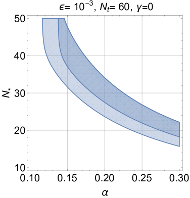
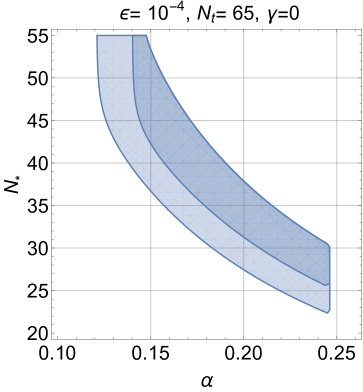
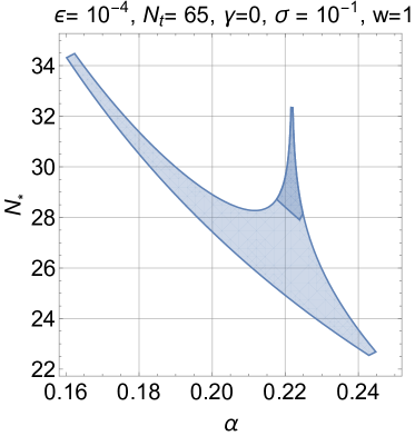
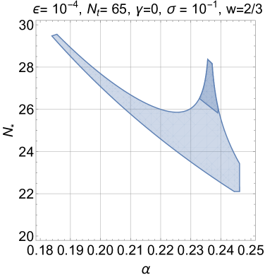
While from the viewpoint of the experiments Eqs. (5.25)–(5.26) are weaker than Eqs. (5.23)–(5.24), from the viewpoint of the signal itself the opposite is true: if we enforce Eqs. (5.23)–(5.24) the allowed region of the parameter space will be larger than in the case of Eqs. (5.25)–(5.26). See, in this respect, Figs. 4 and 5 where we illustrate the constrained parameter space for different choices of the parameters and in the case of a conventional thermal history.
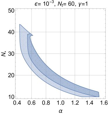
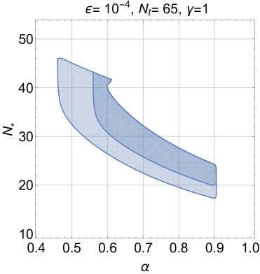
The shaded areas in both plots describe the regions where all the phenomenological constraints are concurrently satisfied while the chirp amplitudes are sufficiently large to be detected. More specifically in Figs. 4 and 5 the outer regions are obtained by enforcing the requirements of Eqs. (5.25) and (5.26). Conversely the inner regions come from the more demanding conditions spelled out in Eqs. (5.23) and (5.24). The reduction of the areas between the outer and the inner regions illustrate the reduction of the parameter space induced by the difference between the requirements of Eqs. (5.23)–(5.24) and (5.25)–(5.26). Note that the case is illustrated in Fig. 4 while Fig. 5 concerns the case . Different values of rescale, in practice, the values of , as expected from the general relation connecting to and . Indeed, to leading order in , the value of is the case is roughly thrice its value in the case. We therefore have that the range of in the two situations must be rescaled by a factor of and this is what we clearly see by comparing the horizontal axes in Figs. 4 and 5.
In the case of a different post-inflationary history the constrained parameter space gets modified and the relevant exclusion plots are illustrated in Fig. 6
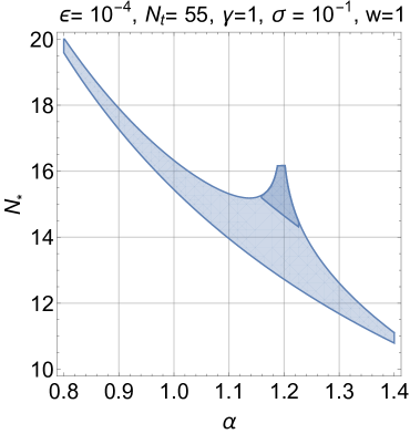
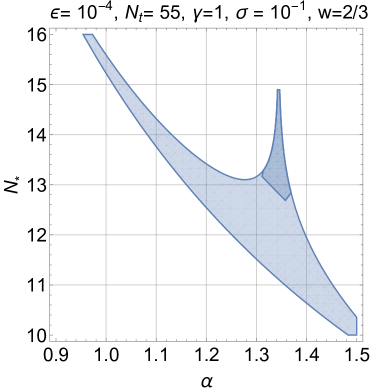
for a fiducial choice of the parameters. In the two plots at the right the barotropic index corresponds to while in the two plots at the left the barotropic index is maximal (i.e. ). By looking at the inner and at the outer exclusion regions we conclude that a reduction in the sensitivities of the hypothetical detectors drastically reduces the areas of the parameter space. Indeed, as in Figs. 4 and 5 the inner and the outer plots correspond, respectively, to the requirements of Eqs. (5.25)–(5.26) and to the requirements of Eqs. (5.23)–(5.24). The reason for this reduction is a direct consequence of the violet spectral slope in the highest frequency domain. Still, for a given value of , the constrained parameter space suggests a potentially interesting signal.
The explicit profiles of different models will now be illustrated. While the same analysis can be easily rephrased either in term of the power spectrum or in terms of the spectral amplitude we shall be mainly interested in the chirp amplitude and in the spectral energy distribution. This kind of approach is also useful for the explicit derivation of a template family.
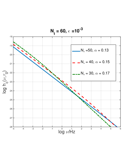
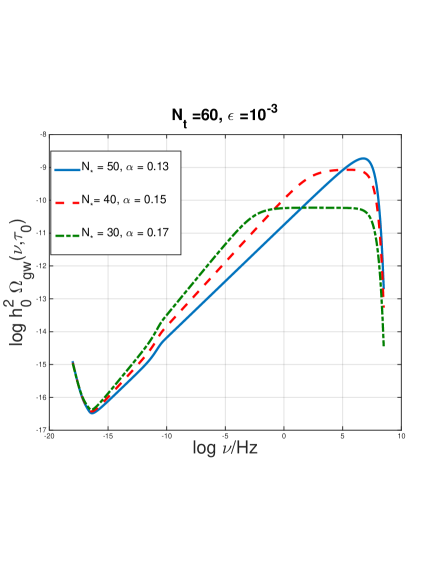
In Fig. 7 we illustrate the chirp amplitude and the spectral energy distribution in the case of a standard post-inflationary history. The scales of the two plots on the horizontal axis are different202020 The chirp amplitude is illustrated in a frequency range encompassing the mHz and the audio bands. Conversely the spectral energy distribution covers all the frequencies from the aHz up to the MHz band.. The explicit differences among the various models are less pronounced if we look at the chirp amplitude which is is proportional to the square root of the spectral energy distribution and it is further suppressed by one power of the frequency. It is finally relevant to stress that Figs. 7, 8 and 9 have been all derived in the case . This is not a limitation, as we saw from the discussion of the constrained parameter space: different values of simply shift the allowed range of . As increases the plateau of Fig. 7 becomes less evident.
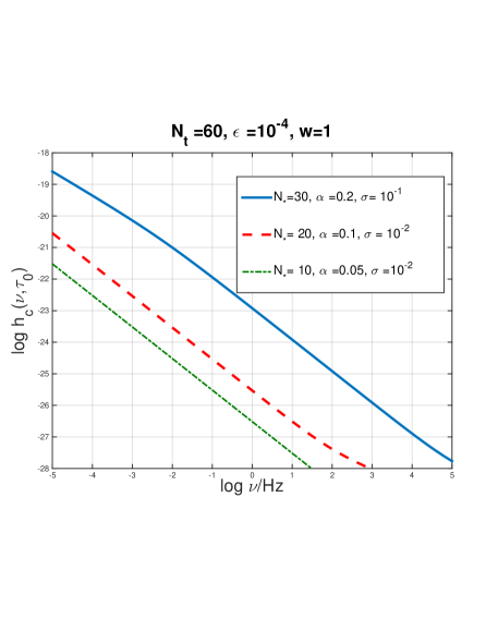
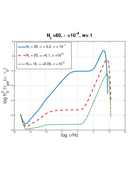
The results of Fig. 7 can be usefully compared with the ones illustrated in Fig. 8 where the post-inflationary evolution is characterized by a stiff epoch. While in Fig. 8 we considered the case , in Fig. 9 we took instead .
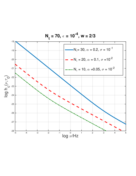
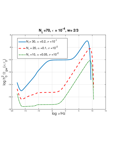
Recalling Eqs. (4.37)–(4.38) and (5.12) the value of the barotropic index controls not only the slope of the cosmic graviton spectrum in the vicinity high-frequency spike but also the frequency range. Larger values of correspond to more violet slopes in the MHz band while the values of are inversely proportional to the frequency of the spike so that as gets smaller than the position of the spike exceeds the GHz. Both and determine the length of the stiff phase.
In the right plots of Figs. 7, 8 and 9 we can appreciate a minor suppression for frequencies of the order of nHz. This suppression is less visible in the chirp amplitude but it is evident from the spectral energy distribution. For the slight break in the spectrum is due to the neutrino free streaming. The neutrinos free stream, after their decoupling, and the effective energy-momentum tensor acquires, to first-order in the amplitude of the plasma fluctuations, an anisotropic stress. The overall effect of collisionless particles is a reduction of the spectral energy density of the relic gravitons. Assuming that the only collisionless species in the thermal history of the Universe are the neutrinos, the amount of suppression can be parametrized by the function
| (5.27) |
where, as usual, is the fraction of neutrinos in the radiation plasma; clearly in the concordance model . In the case (i.e. in the absence of collisionless particles) there is no suppression. If, on the contrary, the suppression can even reach one order of magnitude. In the case , and the suppression of the spectral energy density is proportional to . This suppression due to neutrino free streaming is thus effective for frequencies larger than and smaller than .
Besides neutrino free streaming there are other two minor effects taken into account in Figs. 7, 8 and 9: the damping effect associated with the (present) dominance of the dark energy and the suppression due to the variation of the effective number of relativistic species. In the concordance scenario the redshift of -dominance (i.e. ) determines the numerical value of defined in Eq. (5.7). The adiabatic damping of the mode function due to the dominance of the dark energy implies a damping of the order of in the spectral energy distribution. This suppression competes with a potential increase of the spectral energy distribution for and going as [14, 70]. Finally, for temperatures much larger than the top quark mass, all the known species of the minimal standard model of particle interactions are in local thermal equilibrium, then . Below GeV the various species start decoupling, the notion of thermal equilibrium is replaced by the notion of kinetic equilibrium and the time evolution of the number of relativistic degrees of freedom effectively changes the evolution of the Hubble rate. In principle if a given mode reenters the Hubble radius at a temperature the spectral energy density of the relic gravitons is (kinematically) suppressed by a factor which can be written as [66, 67] where, at the present time, and . So, in the case of the minimal standard model the suppression on will be of the order of . In popular supersymmetric extensions of the minimal standard models and can be as high as, approximately, . This will bring down the figure given above to .
6 Concluding remarks
The evolution of the refractive index during the early stages of a conventional inflationary phase leads to a spectral energy distribution naturally tilted towards frequencies and different post-inflationary thermal histories typically add a further branch to the cosmic graviton spectrum. Overall the spectrum may then exhibit up to four different branches extending between the aHz region and the GHz band. Assuming, in a minimalistic perspective, that the evolution of the refractive index terminates before the end of inflation, the spectral energy distribution involves a quasi-flat plateau at high frequencies that is supplemented by a spike between the MHz and the GHz. Depending on the thermal history the slopes of the spectral energy distribution are red, blue and even violet. After imposing the usual phenomenological constraints, there are still wide portions of the parameter space where the resulting signal could be detectable, at least in principle, either by terrestrial interferometers (in their advanced and enhanced configuration) or by space-borne detectors. In spite of less mundane possibilities leading to growing spectral energy distributions of relic gravitons, the present findings demonstrate that blue and violet spectra are compatible with conventional inflationary scenarios in the presence of a dynamical refractive index.
Acknowledgements
I wish to thank M. Doser, F. Fidecaro, M. Pepe-Altarelli, G. Unal and for interesting exchanges on the topics discussed in this paper. I also thank T. Basaglia, A. Gentil-Beccot and S. Rohr of the CERN Scientific Information Service for their kind assistance.
References
- [1] L. P. Grishchuk, Sov. Phys. JETP 40, 409 (1975) [Zh. Eksp. Teor. Fiz. 67, 825 (1974)].
- [2] L. P. Grishchuk, Annals N. Y. Acad. Sci. 302, 439 (1977).
- [3] L. H. Ford and L. Parker, Phys. Rev. D 16, 1601 (1977).
- [4] B. L. Hu and L. Parker, Phys. Lett. A 63, 217 (1977).
- [5] A. A. Starobinsky, JETP Lett. 30, 682 (1979) [Pisma Zh. Eksp. Teor. Fiz. 30, 719 (1979)].
- [6] V. A. Rubakov, M. V. Sazhin and A. V. Veryaskin, Phys. Lett. 115B, 189 (1982).
- [7] R. Fabbri and M. d. Pollock, Phys. Lett. 125B, 445 (1983).
- [8] L. F. Abbott and M. B. Wise, Nucl. Phys. 224, 541 (1984).
- [9] B. Allen, Phys. rev. D 37, 2078 (1988).
- [10] V. Sahni, Phys. Rev. D 42, 453 (1990).
- [11] L. P. Grishchuk and M. Solokhin, Phys. Rev. D 43, 2566 (1991).
- [12] S. Weinberg, Phys. Rev. D 69, 023503 (2004) [astro-ph/0306304].
- [13] D. A. Dicus and W. W. Repko, Phys. Rev. D 72, 088302 (2005) [astro-ph/0509096].
- [14] W. Zhao and Y. Zhang, Phys. Rev. D 74, 043503 (2006) [astro-ph/0604458].
- [15] M. Giovannini, Phys. Lett. B 668, 44 (2008) [arXiv:0807.1914 [astro-ph]].
- [16] P. A. R. Ade et al. [BICEP2 and Keck Array Collaborations], Phys. Rev. Lett. 116, 031302 (2016) [arXiv:1510.09217 [astro-ph.CO]].
- [17] M. Giovannini, Phys. Lett. B 759, 528 (2016) [arXiv:1603.09217 [astro-ph.CO]].
- [18] G. Hinshaw et al. [WMAP Collaboration], Astrophys. J. Suppl. 208, 19 (2013).
- [19] C. L. Bennett, et.al. [WMAP Collaboration], Astrophys. J. Suppl. 208, 20B (2013).
- [20] W. J. Percival, ıet al. Mon. Not. R. Astron. Soc. 401, 2148 (2010).
- [21] R. Keisler et al., Astrophys. J. 743, 28 (2011).
- [22] J. L. Sievers et al. [Atacama Cosmology Telescope Collaboration], JCAP 1310, 060 (2013).
- [23] P. A. R. Ade et al. [Planck Collaboration], Astron. Astrophys. 594, A13 (2016).
- [24] Y. B. Zeldovich, Mon. Not. Roy. Astron. Soc. 160, 1 (1972).
- [25] B. Spokoiny, Phys. Lett. B 315, 40 (1993).
- [26] M. Giovannini, Phys. Rev. D 58, 083504 (1998); Class. Quant. Grav. 16, 2905 (1999); Phys. Rev. D 60, 123511 (1999).
- [27] P. J. E. Peebles and A. Vilenkin, Phys. Rev. D 59, 063505 (1999); H. Tashiro, T. Chiba and M. Sasaki, Class. Quant. Grav. 21, 1761 (2004); T. J. Battefeld and D. A. Easson, Phys. Rev. D 70, 103516 (2004).
- [28] D. Babusci and M. Giovannini, Phys. Rev. D 60, 083511 (1999); Class. Quant. Grav. 17, 2621 (2000); Int. J. Mod. Phys. D 10, 477 (2001).
- [29] S. Weinberg, Cosmology, (Oxford Univ. Press, Oxford UK, 2008).
- [30] P. Szekeres, Annals Phys. 64, 599 (1971).
- [31] P. C. Peters, Phys. Rev. D 9, 2207 (1974).
- [32] M. Giovannini, Class. Quant. Grav. 33, 125002 (2016) [arXiv:1507.03456 [astro-ph.CO]].
- [33] J. Aasi et al. [LIGO Scientific and VIRGO Collaborations], Phys. Rev. Lett. 113, 231101 (2014) [arXiv:1406.4556 [gr-qc]].
- [34] B. P. Abbott et al. [LIGO Scientific and Virgo Collaborations], Phys. Rev. Lett. 118, 121101 (2017) Erratum: [Phys. Rev. Lett. 119, 029901 (2017)] [arXiv:1612.02029 [gr-qc]].
- [35] J. Aasi et al. [LIGO Scientific Collaboration], Class. Quant. Grav. 32, 074001 (2015) [arXiv:1411.4547 [gr-qc]].
- [36] F. Acernese et al. [VIRGO Collaboration], Class. Quant. Grav. 32, 024001 (2015) [arXiv:1408.3978 [gr-qc]].
- [37] P. Amaro-Seoane et al., GW Notes 6, 4 (2013).
- [38] G. M. Harry, P. Fritschel, D. A. Shaddock, W. Folkner, E. S. Phinney, Class. Quant. Grav. 23 4887 (2006).
- [39] S. Kawamura et al., J. Phys. Conf. Ser. 120, 032004 (2008).
- [40] S. Kawamura et al., Class. Quant. Grav. 28, 094011 (2011).
- [41] Y. Cai, Y. T. Wang and Y. S. Piao, Phys. Rev. D 93, 063005 (2016) [arXiv:1510.08716 [astro-ph.CO]]; Phys. Rev. D 94, 043002 (2016) [arXiv:1602.05431 [astro-ph.CO]].
- [42] M. Giovannini, arXiv:1805.08142 [astro-ph.CO].
- [43] M. Abramowitz and I.A. Stegun, Handbook of Mathematical Functions (Dover, New York, 1972).
- [44] A. Erdelyi, W. Magnus, F. Obehettinger, and F. Tricomi, Higher Trascendental Functions (McGraw-Hill, New York, 1953).
- [45] M. Ando et al., Phys. Rev. Lett. 86, 3950 (2001).
- [46] B. Willke et al., Class. Quant. Grav. 19, 1377 (2002).
- [47] H. Grote [LIGO Scientific Collaboration], Class. Quant. Grav. 27, 084003 (2010).
- [48] Y. Aso et al. [KAGRA Collaboration], Phys. Rev. D 88, 043007 (2013).
- [49] K. Somiya [KAGRA Collaboration], Class. Quant. Grav. 29, 124007 (2012).
- [50] B. Sathyaprakash et al., Class. Quant. Grav. 29, 124013 (2012) Erratum: [Class. Quant. Grav. 30, 079501 (2013)].
- [51] M. Giovannini, Phys. Rev. D 95, 083506 (2017); Phys. Rev. D 96, 101302 (2017).
- [52] Y. Zhang, W. Zhao, T. Xia and Y. Yuan, Phys. Rev. D 74, 083006 (2006) [astro-ph/0508345].
- [53] M. Giovannini, Class. Quant. Grav. 26, 045004 (2009) [arXiv:0807.4317 [astro-ph]]; Phys. Rev. D 82, 083523 (2010) [arXiv:1008.1164 [astro-ph.CO]].
- [54] V. M. Kaspi, J. H. Taylor, and M. F. Ryba, Astrophys. J. 428, 713 (1994).
- [55] F. A. Jenet et al., Astrophys. J. 653, 1571 (2006) [astro-ph/0609013].
- [56] W. Zhao, Phys. Rev. D 83, 104021 (2011) [arXiv:1103.3927 [astro-ph.CO]].
- [57] P. B. Demorest et al., Astrophys. J. 762, 94 (2013) [arXiv:1201.6641 [astro-ph.CO]].
- [58] W. Zhao, Y. Zhang, X. P. You and Z. H. Zhu, Phys. Rev. D 87, 124012 (2013) [arXiv:1303.6718 [astro-ph.CO]].
- [59] R. M. Shannon et al., Science 349, 1522 (2015) [arXiv:1509.07320 [astro-ph.CO]].
- [60] V. F. Schwartzmann, JETP Lett. 9, 184 (1969).
- [61] M. Giovannini, H. Kurki-Suonio and E. Sihvola, Phys. Rev. D 66, 043504 (2002) [astro-ph/0203430].
- [62] R. H. Cyburt, B. D. Fields, K. A. Olive, and E. Skillman, Astropart. Phys. 23, 313 (2005) [astro-ph/0408033].
- [63] M. Dentler, A. Hern ndez-Cabezudo, J. Kopp, P. Machado, M. Maltoni, I. Martinez-Soler and T. Schwetz, arXiv:1803.10661 [hep-ph].
- [64] T. L. Smith, E. Pierpaoli and M. Kamionkowski, Phys. Rev. Lett. 97, 021301 (2006) [astro-ph/0603144]; I. Sendra and T. L. Smith, Phys. Rev. D 85, 123002 (2012) [arXiv:1203.4232 [astro-ph.CO]].
- [65] M. Giovannini, Phys. Rev. D 89, 123517 (2014) [arXiv:1404.7333 [hep-th]].
- [66] M. Giovannini, Class. Quant. Grav. 31, 225002 (2014) [arXiv:1405.6301 [astro-ph.CO]].
- [67] M. Giovannini, Phys. Lett. B 759, 528 (2016) [arXiv:1603.09217 [astro-ph.CO]].
- [68] M. S. Turner, M. J. White and J. E. Lidsey, Phys. Rev. D 48, 4613 (1993).
- [69] S. Chongchitnan and G. Efstathiou, Phys. Rev. D 73, 083511 (2006) [astro-ph/0602594]; Prog. Theor. Phys. Suppl. 163, 204 (2006).
- [70] Y. Zhang, X. Z. Er, T. Y. Xia, W. Zhao and H. X. Miao Class. Quantum Grav. 23 3783 (2006).