The clustering of galaxies in the completed SDSS-III Baryon Oscillation Spectroscopic Survey: a tomographic measurement of structure growth and expansion rate from anisotropic galaxy clustering in Fourier space

Abstract

We perform a tomographic structure growth and expansion rate analysis using the monopole, quadrupole and hexadecapole of the redshift-space galaxy power spectrum derived from the Sloan Digital Sky Survey (SDSS-III) Baryon Oscillation Spectroscopic Survey (BOSS) Data Release 12 combined sample, which covers the redshift range of $0.20<z<0.75$. By allowing for overlap between neighbouring redshift slices in order to extract information on the light-cone, we successfully obtain joint BAO and RSD constraints with a precision of $2-3\%$ for $D_{A}$, $3-10\%$ for $H$ and $9-12\%$ for $f\sigma_{8}$ with a redshift resolution of $\Delta z\sim 0.04$. Our measurement is consistent with that presented in Wang et al. (2018b), where the analysis is performed in configuration space. We apply our measurement to constrain the $f(R)$ gravity model, and find that the 95% CL upper limit of ${\rm log_{10}}B_{0}$ can be reduced by 11% by our tomographic BAO and RSD measurement. We make our joint BAO and RSD measurement publicly available at https://github.com/Alice-Zheng/RSD-data

1 Introduction

Physics behind the accelerating expansion of the Universe, which was discovered in 1998 (Riess et al., 1998; Perlmutter et al., 1999), remains unveiled. In principle, introducing dark energy (DE) as a dominating energy component of the Universe at the current epoch (see Weinberg et al. 2013 for a recent review on dark energy), or extending Einstein’s general relatively on cosmological scales, dubbed the modified gravity (MG) scenario (see Koyama 2016 for a recent review on modified gravity), can be possible origins of the cosmic acceleration. Although these two scenarios can be degenerate at the level of the cosmic expansion, they are distinguishable at the level of structure formation. Observationally, large spectroscopic galaxy surveys offer key probes for both DE and MG through measurements of specific three-dimensional patterns of galaxy clustering including the Baryonic Acoustic Oscillations (BAO) and Redshift Space Distortions (RSD).

The observable of BAO is the excess in galaxy clustering at about 150 $\,\rm Mpc$ on the comoving scale, which is due to the interaction between photons and baryons in the early universe (Peebles & Yu, 1970). The BAO scale can be derived from two-point correlation functions or power spectra multipoles of galaxies in redshift space. By virtue of the Alcock-Paczynski (AP) effect (Alcock & Paczynski, 1979), which quantifies a difference of the BAO distance scales between radial and transverse directions due to an improper choice of the ‘fiducial’ cosmology to convert redshifts to distances, the Hubble parameter and the angular diameter distance at an effective redshift $z$, $H(z)$ and $D_{A}(z)$ respectively, can be estimated from the anisotropic galaxy clustering. As the BAO scale is largely immune to systematics (Ross et al., 2011), it has been widely used as a standard ruler to probe the expansion history of the Universe, facilitating a power tool for the study of DE.

RSD produce another kind of anisotropy in the galaxy clustering. Unlike the AP effect, RSD are due to peculiar motions of galaxies affected by local gravitational potentials. As the galaxy clustering is observed in redshift space, in which the peculiar motions only alter the clustering along the line of sight, an anisotropy in the galaxy clustering is produced, which is directly related to gravity. In the linear regime, RSD yield an angle-dependent boost of the power spectrum amplitude by a factor of $(1+\beta\mu^{2})^{2}$ (Kaiser, 1987), where $\mu$ is the cosine of the angle between the galaxy pair and the line-of-sight vectors, and $\beta\equiv f/b$, the ratio between the growth rate $f$ and the galaxy bias $b$. This provides a direct measure of the growth rate of the Universe, which is one of the key probes of gravity on cosmological scales.

Joint measurements of BAO and RSD can in principle break the ‘dark degeneracy’ between DE and MG, which is key to understand the cosmic acceleration. In order to maximise the BAO and RSD information extracted from the survey volume, methods of tomographic analysis on the lightcone have been developing, including the overlapping redshift slicing method (Zhao et al., 2017b; Wang et al., 2018b; Wang et al., 2017) and optimal redshift weighting schemes (Zhu et al., 2015; Zhu et al., 2016; Ruggeri et al., 2017; Ruggeri et al., 2018; Wang et al., 2018a; Zhao et al., 2019; Zhu et al., 2018). As demonstrated in Zhao et al. (2017a) and Zhao et al. (2019), these methods can effectively extract additional information on the lightcone, which generically improves constraints on dark energy and modified gravity. The optimal redshift weighting method is more computationally efficient, as it allows for measuring the linear combinations of power spectra at various redshifts, which are most sensitive to the cosmological parameters, without subdividing the galaxy sample. However, it requires a robust modelling of the time evolution of key cosmological quantities including the BAO, RSD, the bias, etc. in the first place, which can be theoretically challenging. On the other hand, the overlapping redshift slicing method is more computationally expensive, but it does not require an assumption of the temporal evolution of the system, which is less subject to theoretical systematics.

In this work, we apply the overlapping redshift slicing method developed in Zhao et al. (2017b); Wang et al. (2018b); Wang et al. (2017) to the BAO and RSD analysis in Fourier space using the BOSS DR12 galaxy catalog, and make cosmological implications. This paper is structured as follows. In Section 2, we describe the methodology in our analysis, including the galaxy and mock catalogs used for this analysis, the theoretical template and details for parameter estimation. In Section 3, we show the main results including the mock tests, tomographic measurements of BAO and RSD parameters, as well as a cosmological implication on observational constraints on the $f(R)$ gravity. The last section is devoted to conclusion and discussions.

2 Methodology

In this section, we describe the data used in this analysis (including the galaxy and mock catalogs), the theoretical template for the joint BAO and RSD measurement, and the method used for parameter estimation.

2.1 The Data

The observational dataset used in this work is obtained by the Sloan Digital Sky Survey (SDSS-III) Baryon Oscillation Spectroscopic Survey (BOSS). Using a $2.5$ metre-aperture Sloan Foundation Telescope (Gunn et al., 2006) at the Apache Point Observatory, the BOSS program covers around 10, 000 square degrees of the sky. The BOSS team has obtained spectra of over 1.5 million galaxies brighter than $i=19.9$ and approximately 170, 000 new quasars in the redshift range of $z\in[2.1,3.5]$. The spectrograph, filter and pipeline of BOSS are described in Fukugita et al. (1996); Bolton et al. (2012); Smee et al. (2013).

The galaxy catalogue for this analysis is built upon the BOSS Data Release (DR) 12 combined sample, which is a coherent combination of two distinct targets of LOWZ and CMASS. The stellar-mass incompleteness of the LOWZ and CMASS samples was discussed in Leauthaud et al. (2016), and its impact on the clustering was studied in Saito et al. (2016) and Rodríguez-Torres et al. (2016). The DR12 combined catalogue was reduced from observations using the pipeline described in Reid et al. (2016), where the survey footprint, veto masks and survey systematics are taken into account when creating the data and random catalogues. The redshift range of this sample is $z\in[0.2,0.75]$, containing approximately $865,000$ and $330,000$ galaxies in the North Galactic Cap (NGC) and South Galactic Cap (SGC) respectively.

For the purpose of estimating the data covariance matrix, and of validating our data analysis pipeline, mock galaxy catalogues are required. In this work, we use the MultiDark-Patchy (MD-Patchy) mock catalogue (Kitaura et al., 2016), which offers 2048 realisations of mock galaxy distributions, matching the spatial and redshift distribution of the DR12 combined sample. As demonstrated in Kitaura et al. (2016), the Patchy mocks accurately reproduce the two-point and three-point statistics of galaxy clustering in the BOSS DR12 sample, which validates it for the use of likelihood analysis for the DR12 sample. The light-cone of the Patchy mocks was constructed using ten redshift slices, which permits the determination the time evolution of the galaxy bias, the growth, and the peculiar motion. We refer to Kitaura et al. (2016) for more details of the implementation of the light-cone construction.

The fiducial cosmology used in the analysis is the same as that used for producing the Patchy mocks, namely,

$$\left\{\Omega_{\rm M},\Omega_{\rm b},\Omega_{\rm K},h,\sigma_{8}\right\}=\left\{0.307115,0.0480,0,0.6777,0.8288\right\}$$ (1)

which is consistent with the results from the Planck collaboration (Planck Collaboration et al., 2016).

2.2 The overlapping redshift slicing

To extract information from the past lightcone of the survey, we adopt the overlapping redshift slicing (ORS) method developed and applied in Zhao et al. (2017b); Wang et al. (2018b); Wang et al. (2017). The essence of the ORS method is to subdivide the galaxy sample into numerous overlapping redshift slices, in order to guarantee that the number of galaxies in each redshift slice is sufficiently large to yield a decent BAO and RSD measurement, and that the redshift slicing is sufficiently fine so that the key tomographic information on the lightcone is extracted. In Zhao et al. (2017b); Wang et al. (2018b); Wang et al. (2017), where the same galaxy and mock catalogues are used for BAO and/or RSD analyses (see Table 1 for details of these analyses), the DR12 combined sample was subdivided into nine overlapping redshift slices, as detailed in Table 2. As detailed in Zhao et al. (2017b), our redshift-slicing scheme can well balance the redshift resolution and the complementarity of the information between overlapping bins, and an analysis of RSD in configuration space using the same redshift binning has demonstrated the effectiveness of our binning scheme (Wang et al., 2018b). In this work, we adopt the same ORS for a joint BAO and RSD analysis in Fourier space, which is complementary to the joint BAO and RSD analysis in configuration space performed in Wang et al. (2018b)

Analysis	Reference
BAO in $s$-space	Wang et al. (2017)
BAO in $k$-space	Zhao et al. (2017b)
BAO+RSD in $s$-space	Wang et al. (2018b)
BAO+RSD in $k$-space	This work

Table 1: A list of tomographic BAO or RSD analyses using the overlapping redshift slicing shown in Table 2.

redshift bin index	redshift range	effective $z$
$z$ bin 1	$0.20<z<0.39$	0.31
$z$ bin 2	$0.28<z<0.43$	0.36
$z$ bin 3	$0.32<z<0.47$	0.40
$z$ bin 4	$0.36<z<0.51$	0.44
$z$ bin 5	$0.40<z<0.55$	0.48
$z$ bin 6	$0.44<z<0.59$	0.52
$z$ bin 7	$0.48<z<0.63$	0.56
$z$ bin 8	$0.52<z<0.67$	0.59
$z$ bin 9	$0.56<z<0.75$	0.64

Table 2: The overlapping redshift slicing applied on the DR12 combined sample for analyses shown in Table 1.

2.3 Measurements of the power spectrum multipoles

As we use the same redshift slicing scheme as that in Zhao et al. (2017b) for this analysis, we use the power spectrum multipoles (up to the hexadecapole) measured in Zhao et al. (2017b) using a Fast Fourier Transformations (FFTs) method (Bianchi et al., 2015). For the measurement, galaxies and random catalogues are placed in a cubic box with $L=5000\ h^{-1}$ Mpc a side, which is divided into $1024^{3}$ cubic cells for calculating the over-density field, and for the FFTs, and we follow the prescription developed in Jing (2005) to correct for the aliasing effect of the FFTs.

2.4 The template

2.4.1 Modelling the power spectrum in redshift space

We use the extended TNS (eTNS) prescription (Taruya et al., 2010) to model the anisotropic power spectrum in redshift space, as implemented for the RSD analyses in Fourier space using datasets of BOSS DR12 (Beutler et al., 2017b) and eBOSS DR14 (Zhao et al., 2019; Gil-Marín et al., 2018).

The eTNS model reads,

$$\begin{split}P_{\rm g}(k,\mu)&=e^{-(fk\mu\sigma_{v})^{2}}\left[P_{{\rm g},\delta\delta}(k)\right.\\ &\;\;\;+2f\mu^{2}P_{{\rm g},\delta\theta}(k)+f^{2}\mu^{4}P_{\theta\theta}(k)\\ &\;\;\;+b_{1}^{3}\sum_{m,n=1}^{3}\,\mu^{2m}\,\beta^{n}A_{mn}\\ &\;\;\;+b_{1}^{4}\sum^{4}_{n=1}\sum^{2}_{a,b=1}\mu^{2n}\left(-\beta\right)^{a+b}\left.B^{n}_{ab}\right]\end{split}$$ (2)

where $f\equiv\frac{d\ln D\left(a\right)}{d\ln a}$ denotes the logarithmic growth rate, $\mu$ is the cosine of the angle between the wavenumber vector $k$ and the line-of-sight direction, and $\sigma_{v}$ is treated as a free parameter to be marginalised over.

The overall exponential damping factor in Eq (2) encodes the Fingers-of-God (FoG) effect. The terms in the square brackets extend the linear Kaiser model, where the first three terms are auto- and cross-power spectra of the matter density field $\delta$ and of the divergence of the peculiar velocity field $\theta$, while the the last two (the A and B) terms correct for higher-order correlations. We compute the power spectra terms using the regularised perturbation theory (RegPT) up to second order (Taruya et al., 2012) , and calculate the A and B terms using the standard perturbation theory (SPT) (Taruya et al., 2010). Note that all these terms except for $P_{\theta\theta}(k)$ contain the the linear bias $b_{1}$ and the local non-linear bias $b_{2}$ .

2.4.2 The Alcock-Paczynski effect

The Alcock-Paczynski (AP) effect (Alcock & Paczynski, 1979) changes the galaxy clustering due to the incorrect input cosmology to convert redshifts to distances. Mathematically, it alters the anisotropic galaxy clustering shown in Eq (2) in the following way (Ballinger et al., 1996),

$$P_{g}(k,\mu)\rightarrow P_{g}(k^{\prime},\mu^{\prime}),$$ (3)

where

$$k^{\prime}=\frac{k}{\alpha_{\perp}}\left[1+\mu^{2}\left(\frac{1}{F^{2}}-1\right)\right]^{1/2},$$

$$\mu^{\prime}=\frac{\mu}{F}\left[1+\mu^{2}\left(\frac{1}{F^{2}}-1\right)\right]^{-1/2},$$

$$F=\alpha_{\parallel}/\alpha_{\perp}.$$ (4)

Then the power spectrum multipoles can be calculated as,

$$P_{\rm\ell}(k) =\left(\frac{r_{s}^{\rm fid}}{r_{s}}\right)^{3}\frac{(2\ell+1)}{2\alpha^{2}_{\perp}\alpha_{\parallel}}\int^{1}_{-1}d\mu\;P_{\rm g}\left(k^{\prime},\mu^{\prime}\right)\mathcal{L}_{\ell}(\mu),$$ (5)

where $r_{s}$ denotes the sound horizon at the recombination. The factor $\left(\frac{r_{s}^{\rm fid}}{r_{s}}\right)^{3}\frac{1}{2\alpha^{2}_{\perp}\alpha_{\parallel}}$ accounts for the difference in the cosmic volume in different cosmologies (Beutler et al., 2017a).

2.4.3 The survey window function

Due to the irregularity and the finite size of the survey volume of the BOSS survey, the observed power spectrum is the theoretical power spectrum convolved with the window function. We follow the method developed in Wilson et al. (2017), which is an efficient way to reduce the three-dimensional convolutions to one-dimensional Hankel transformations, which can be done rapidly using the FFTlog algorithm (Hamilton, 2000a). We refer to Zhao et al. (2017b) for more details on the convolution of the survey window function for the ORS used in this work, and for details on how to convolve the window function of the survey with the model; briefly we follow the method developed in Wilson et al. (2015) and make use of FFTlog libraries (Hamilton, 2000b). The window functions used for this analysis are identical to those shown in Fig. 9 in Zhao et al. (2017b).

2.5 The parameter estimation

As the target selection is slightly different for the North Galactic Cap (NGC) and in the South Galactic Cap (SGC), We treat the two areas separately (Beutler et al., 2017b; Zhao et al., 2017b), which leaves eleven free parameters to be determined for each redshift slice.

For a given set of parameters, we use a modified version of CAMB (Lewis et al., 2000) to compute the theoretical prediction, and then use CosmoMC (Lewis & Bridle, 2002) to sample the parameter space using the Monte Carlo Markov Chain (MCMC) method. The likelihood function to be maximised by CosmoMC is,

$$\chi^{2}(\mathbb{p})\equiv\sum_{i,j}^{\ell,\ell^{\prime}}\left[P^{\rm d}_{\ell}(k_{i},\mathbb{p})-P^{\rm th}_{\ell}(k_{i})\right]F^{\ell,\ell^{\prime}}_{ij}\left[P_{\ell^{\prime}}^{\rm d}(k_{j},\mathbb{p})-P^{\rm th}_{\ell^{\prime}}(k_{j})\right]$$

where superscripts ^d and ^th denote data and theoretical prediction respectively, ${\bf p}$ stands for a collection of parameters shown in Table 3, and $F^{\ell,\ell^{\prime}}_{ij}$ is the inverse of the data covariance matrix estimated from the Patchy mock catalogues. We use the power spectrum measurement in the wavenumber range of $k\in[0.015,0.15]h\ {\rm Mpc^{-1}}$ to avoid contaminant from both observational and theoretical systematics (Beutler et al., 2017b). We follow Percival et al. (2014) to perform a rescaling of the uncertainty of each parameter returned by MCMC, to correct for the fact that finite number of mocks are used to estimate the data covariance matrix.

Parameter	Meaning	Prior
$\alpha_{\parallel}$	The radial BAO dilation parameter	[0.8,1.2]
$\alpha_{\perp}$	The transverse BAO dilation parameter	[0.8,1.2]
$f\sigma_{8}$	The RSD parameter	[0, 1]
$b_{1}^{\rm NGC}\sigma_{8}$	The linear bias for the NGC	[0.5,2.1]
$b_{2}^{\rm NGC}\sigma_{8}$	The nonlocal bias for the NGC	[0,4]
$\sigma_{v}^{\rm NGC}$	The velocity dispersion for the NGC	[1,9]
$N^{\rm NGC}$	The correction to the shot noise for NGC	[-2000,2000]
$b_{1}^{\rm SGC}\sigma_{8}$	The linear bias for the SGC	[0.5,2.1]
$b_{2}^{\rm SGC}\sigma_{8}$	The nonlocal bias for the SGC	[0,4]
$\sigma_{v}^{\rm SGC}$	The velocity dispersion for the SGC	[1,9]
$N^{\rm SGC}$	The correction to the shot noise for SGC	[-2000,2000]

Table 3: The free parameters, physical meaning and the flat priors used in the MCMC analysis for each redshift slice.

3 Results

Table 4: Measurements (mean with the 68% CL uncertainty) of BAO and RSD parameters including $\alpha_{\perp}$, $\alpha_{\parallel}$ and $f\sigma_{8}$ using $P_{0}+P_{2}$ (left part of the table) and $P_{0}+P_{2}+P_{4}$ (right) derived from the mock catalogues at nine effective redshifts. As a mock test, the absolute values of differences between the measurement and the expected values are shown. All measurements are multiplied by a factor of $100$ for illustration.

		Mock catalogue $\left(P_{0}+P_{2}\right)$			Mock catalogue $\left(P_{0}+P_{2}+P_{4}\right)$
$z_{\rm eff}$	$\Delta\alpha_{\parallel}$	$\Delta\alpha_{\perp}$	$\Delta f\sigma_{8}$	$\Delta\alpha_{\parallel}$	$\Delta\alpha_{\perp}$	$\Delta f\sigma_{8}$
0.31	$0.10\pm 3.93$	$0.48\pm 3.56$	$2.71\pm 6.82$	$0.99\pm 3.73$	$0.48\pm 3.41$	$1.59\pm 5.77$
0.36	$0.68\pm 3.70$	$0.20\pm 3.29$	$3.73\pm 7.48$	$0.86\pm 3.30$	$0.31\pm 2.97$	$1.67\pm 5.42$
0.40	$0.58\pm 3.56$	$1.52\pm 3.08$	$1.73\pm 6.42$	$0.28\pm 3.02$	$0.24\pm 2.68$	$1.42\pm 5.36$
0.44	$0.89\pm 3.70$	$1.74\pm 3.07$	$1.63\pm 5.28$	$0.48\pm 2.94$	$0.26\pm 2.58$	$0.21\pm 5.12$
0.48	$1.04\pm 3.67$	$0.87\pm 2.73$	$0.05\pm 6.86$	$0.71\pm 2.72$	$0.56\pm 2.35$	$0.25\pm 4.85$
0.52	$0.85\pm 2.53$	$0.73\pm 2.31$	$0.55\pm 5.35$	$0.82\pm 2.52$	$0.21\pm 2.17$	$0.57\pm 4.48$
0.56	$0.64\pm 3.80$	$1.81\pm 2.99$	$3.61\pm 6.34$	$0.95\pm 2.42$	$0.26\pm 2.09$	$0.58\pm 4.24$
0.59	$0.73\pm 3.78$	$0.92\pm 2.82$	$1.89\pm 5.23$	$0.11\pm 2.34$	$0.39\pm 2.00$	$0.91\pm 4.24$
0.64	$1.67\pm 3.63$	$0.82\pm 2.79$	$3.92\pm 7.43$	$0.15\pm 2.27$	$0.70\pm 1.90$	$0.43\pm 4.40$

In this section, we present our joint tomographic BAO and RSD measurement from the BOSS DR12 combined sample, after validating our pipeline using the Patchy mock catalogue. We then perform a cosmological implication of our BAO and RSD measurement on the $f(R)$ gravity, and summarise the result.

3.1 Pipeline validation using the Patchy mocks

To validate our pipeline, we perform a joint BAO and RSD analysis on the Patchy mock catalogues, which are also subdivided into nine overlapping redshift slices detailed in Table 2. We measure the BAO and RSD parameters (with other relevant parameters marginalised over) from the average of the power spectra multipoles derived from $2048$ Patchy mocks, and show the result in Table 4. As this is a mock test, which is used to validate our pipeline by checking whether we can reproduce the values of cosmological parameters used to create the mocks, we show the absolute values of the difference (multiplied by $100$ for the ease of visulisation) between the measurements and the values expected.

To check the agreement between our measurement and expected values, we further define two quantities, namely the fractional bias $\Delta p/p$, and the fractional increase in the total uncertainty $\Delta\sigma_{p}/\sigma_{p}$,

$$\Delta p/p\equiv\max_{\forall z_{i}\in Z_{9}}\ \left|p_{z_{i}}/p_{z_{i},{\rm fid}}-1\right|,$$ (6)

$$\Delta\sigma_{p}/\sigma_{p}\equiv\max_{\forall z_{i}\in Z_{9}}\left[\left(p_{z_{i}}-p_{z_{i},{\rm fid}}\right)^{2}/\sigma_{p,{z_{i}}}^{2}+1\right]^{1/2}-1.$$ (7)

where the set $p$ includes BAO and RSD parameters, i.e., $p\equiv\left\{\alpha_{\parallel},\alpha_{\perp},f\sigma_{8}\right\}$, and the set $Z_{9}$ is a collection of nine effective redshifts for this analysis, as shown in Table 2.

As defined, $\Delta p/p$ is the fractional measurement bias of the parameters, while $\Delta\sigma_{p}/\sigma_{p}$ quantifies the fractional increase in the total uncertainty of parameters due to the bias in the measurement. Note that we estimate the total uncertainty of a parameter by adding the bias and statistical uncertainty in quadrature, i.e.,

$$\sigma_{p}=\sqrt{\left(p-p_{\rm fid}\right)^{2}+\sigma^{2}_{\rm stat}}$$ (8)

Note that $\Delta p/p$ and $\Delta\sigma_{p}/\sigma_{p}$ are maximal values of the fractional measurement bias, and of the fractional increase in the total uncertainty respectively, across all the redshift slices.

We list $\Delta p/p$ and $\Delta\sigma_{p}/\sigma_{p}$ derived from monopole and quadrupole $(P_{0}+P_{2})$, and from monopole, quadrupole and hexadecapole $(P_{0}+P_{2}+P_{4})$ in Table 5. As shown, using $P_{0}+P_{2}$, the bias for $f\sigma_{8}$ is around $8\%$, although a higher level of agreement is reached for $\alpha_{\parallel}$ and $\alpha_{\perp}$, namely, the biases for these parameters never exceed $2\%$ in all redshift slices. However, the biases can dilute the total uncertainties by up to 17%. Adding hexadecapole to the analysis, however, significantly reduces the bias, which avoids inflating the total error budget to a noticeable amount (Beutler et al., 2017b). Specifically, the biases of the BAO parameters are reduced to sub-percent level, and the bias of $f\sigma_{8}$ drops by more than a factor of $2$. More importantly, $\Delta\sigma_{p}/\sigma_{p}$ is pushed below $8\%$ in all cases, which means that the systematic error budget is negligible compared with the statistical errors.

This mock test validates our pipeline, as we successfully recover the BAO and RSD parameters from the average of mock catalogues, with a negligible bias and impact on the total uncertainty when monopole, quadrupole and hexadecapole are used for the analysis.

Table 5: The fractional bias $\Delta p/p$ defined in Eq (6) and the fractional increase in the total uncertainty $\Delta\sigma_{p}/\sigma_{p}$ defined in Eq (7) of parameters $\alpha_{\parallel},\alpha_{\perp}$ and $f\sigma_{8}$ derived from $P_{0}+P_{2}$ (left part) and $P_{0}+P_{2}+P_{4}$ (right) respectively.

	Mock catalogue $\left(P_{0}+P_{2}\right)$		Mock catalogue $\left(P_{0}+P_{2}+P_{4}\right)$
	$\Delta p/p$	$\Delta\sigma_{p}/\sigma_{p}$	$\Delta p/p$	$\Delta\sigma_{p}/\sigma_{p}$
$\alpha_{\parallel}$	$1.7\%$	$10.1\%$	$0.99\%$	$7.4\%$
$\alpha_{\perp}$	$1.8\%$	$16.9\%$	$0.70\%$	$6.6\%$
$f\sigma_{8}$	$8.3\%$	$15.1\%$	$3.5\%$	$4.6\%$

Table 6: Measurements (mean with the 68% CL uncertainty) of BAO and RSD parameters including $\alpha_{\perp}$, $\alpha_{\parallel}$ and $f\sigma_{8}$ using $P_{0}+P_{2}$ (left part of the table) and $P_{0}+P_{2}+P_{4}$ (right) derived from the BOSS DR12 catalogue at nine effective redshifts. The $\chi^{2}/\nu$ columns show the reduced $\chi^{2}$, where $\nu$ is the number of degrees of freedom.

	DR12 $\left(P_{0}+P_{2}\right)$				DR12 $\left(P_{0}+P_{2}+P_{4}\right)$
$z_{\rm eff}$	$\alpha_{\parallel}$	$\alpha_{\perp}$	$f\sigma_{8}$	$\chi^{2}/\nu$	$\alpha_{\parallel}$	$\alpha_{\perp}$	$f\sigma_{8}$	$\chi^{2}/\nu$
0.31	$0.990\pm 0.037$	$1.022\pm 0.032$	$0.437\pm 0.054$	$56/45$	$1.000\pm 0.034$	$1.021\pm 0.032$	$0.452\pm 0.053$	$65/73$
0.36	$0.965\pm 0.042$	$1.005\pm 0.025$	$0.442\pm 0.057$	$59/45$	$0.984\pm 0.028$	$1.006\pm 0.025$	$0.450\pm 0.054$	$73/73$
0.40	$0.956\pm 0.049$	$0.994\pm 0.033$	$0.459\pm 0.062$	$64/45$	$0.977\pm 0.033$	$0.996\pm 0.030$	$0.461\pm 0.055$	$80/73$
0.44	$0.967\pm 0.038$	$1.023\pm 0.035$	$0.472\pm 0.071$	$61/45$	$1.007\pm 0.027$	$1.024\pm 0.025$	$0.480\pm 0.052$	$90/73$
0.48	$0.989\pm 0.037$	$1.034\pm 0.041$	$0.482\pm 0.070$	$71/45$	$1.020\pm 0.026$	$1.045\pm 0.021$	$0.469\pm 0.052$	$83/73$
0.52	$1.007\pm 0.038$	$1.051\pm 0.024$	$0.478\pm 0.064$	$70/45$	$1.031\pm 0.027$	$1.048\pm 0.024$	$0.483\pm 0.042$	$84/73$
0.56	$0.995\pm 0.033$	$1.036\pm 0.022$	$0.476\pm 0.058$	$70/45$	$1.008\pm 0.026$	$1.032\pm 0.022$	$0.471\pm 0.045$	$72/73$
0.59	$0.965\pm 0.046$	$1.013\pm 0.020$	$0.445\pm 0.062$	$75/45$	$0.991\pm 0.024$	$1.010\pm 0.021$	$0.435\pm 0.042$	$75/73$
0.64	$0.958\pm 0.038$	$1.015\pm 0.019$	$0.421\pm 0.067$	$54/45$	$0.988\pm 0.025$	$1.014\pm 0.019$	$0.426\pm 0.046$	$69/73$

Table 7: Mean and the 68% CL uncertainty on BAO and AP parameters derived from $P_{0}+P_{2}$ (left part of the table) and $P_{0}+P_{2}+P_{4}$ (right) using the BOSS DR12 catalogue at nine effective redshifts. The unit for $D_{\rm A}$ and $D_{\rm V}$ is Mpc, and is $\rm km\,s^{-1}Mpc^{-1}$ for $H$. $F_{\rm AP}$ is dimensionless.

		DR12 $\left(P_{0}+P_{2}\right)$				DR12 $\left(P_{0}+P_{2}+P_{4}\right)$
$z_{\rm eff}$	$D_{\rm A}\left({r_{\rm s}^{\rm fid}}/{r_{\rm s}}\right)$	$H\left({r_{\rm s}}/{r_{\rm s}^{\rm fid}}\right)$	$D_{\rm V}\left({r_{\rm s}^{\rm fid}}/{r_{\rm s}}\right)$	$F_{\rm AP}$	$D_{\rm A}\left({r_{\rm s}^{\rm fid}}/{r_{\rm s}}\right)$	$H\left({r_{\rm s}}/{r_{\rm s}^{\rm fid}}\right)$	$D_{\rm V}\left({r_{\rm s}^{\rm fid}}/{r_{\rm s}}\right)$	$F_{\rm AP}$
0.31	$986\pm 31$	$80.5\pm 5.8$	$1250\pm 33$	$0.349\pm 0.025$	$992\pm 28$	$79.7\pm 4.2$	$1198\pm 32$	$0.348\pm 0.023$
0.36	$1074\pm 27$	$85.2\pm 9.4$	$1394\pm 31$	$0.415\pm 0.021$	$1075\pm 26$	$83.5\pm 8.9$	$1394\pm 29$	$0.341\pm 0.019$
0.40	$1139\pm 38$	$87.9\pm 7.2$	$1514\pm 41$	$0.467\pm 0.042$	$1141\pm 33$	$86.0\pm 6.5$	$1514\pm 37$	$0.468\pm 0.039$
0.44	$1243\pm 32$	$89.0\pm 3.4$	$1681\pm 35$	$0.531\pm 0.036$	$1245\pm 30$	$85.5\pm 2.7$	$1681\pm 32$	$0.530\pm 0.034$
0.48	$1330\pm 27$	$89.2\pm 4.0$	$1843\pm 29$	$0.586\pm 0.025$	$1331\pm 25$	$86.5\pm 3.7$	$1843\pm 29$	$0.508\pm 0.023$
0.52	$1392\pm 32$	$89.6\pm 7.8$	$1983\pm 34$	$0.632\pm 0.026$	$1387\pm 31$	$87.5\pm 6.8$	$1946\pm 33$	$0.582\pm 0.024$
0.56	$1419\pm 30$	$92.9\pm 7.9$	$2070\pm 33$	$0.686\pm 0.024$	$1413\pm 28$	$91.7\pm 6.1$	$2013\pm 32$	$0.687\pm 0.023$
0.59	$1430\pm 29$	$97.6\pm 4.9$	$2108\pm 31$	$0.740\pm 0.023$	$1425\pm 28$	$95.0\pm 3.2$	$2102\pm 29$	$0.739\pm 0.021$
0.64	$1482\pm 28$	$101.1\pm 3.4$	$2239\pm 28$	$0.819\pm 0.022$	$1479\pm 26$	$98.0\pm 3.2$	$2201\pm 27$	$0.713\pm 0.020$

3.2 BAO and RSD measurement from the DR12 combined sample

We apply our validated pipeline to the DR12 combined sample, and show the measurement of BAO and RSD parameters in Tables 6 and 7, and in Figures 1, 2, 4 and 3.

Table 6 and Figure 1 show the constraints on $\alpha_{\parallel},\alpha_{\perp}$ and $f\sigma_{8}$ derived from $P_{0}+P_{2}$ and $P_{0}+P_{2}+P_{4}$ respectively. As shown, $P_{4}$ can significantly improve the constraint on all three parameters, especially for redshift slices $5,6,7$ and $8$, in which $P_{4}$ is measured with relatively higher signal to noise ratio (SNR). Specifically, $\alpha_{\parallel},\alpha_{\perp}$ and $f\sigma_{8}$ are measured with a precision of $3-5\%,2-3\%$ and $12-16\%$ respectively, depending on the effective redshift, using $P_{0}+P_{2}$, and the precision is improved to $2-3\%,2-3\%$ and $9-12\%$ when $P_{4}$ is added to the analysis. As demonstrated in the mock test in Sec. 3.1, analysis with $P_{4}$ included is not only more precise, but also more robust against systematics in the pipeline, we therefore regard our measurement derived from $P_{0}+P_{2}+P_{4}$ as the main result of this work, and use it for comparison with other works and for cosmological implications.

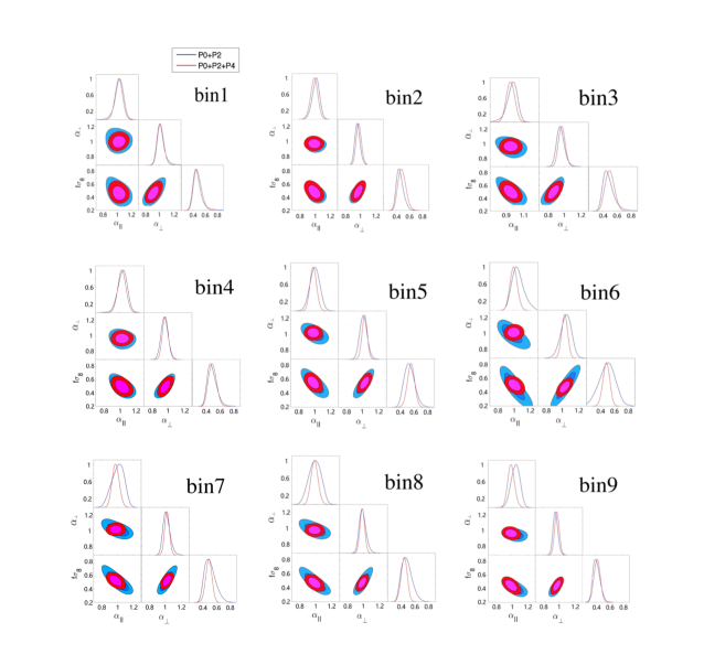
Figure 1: The one-dimensional posterior distribution and 68 and 95 % CL contour plots for parameters $\alpha_{\perp}$, $\alpha_{\parallel}$ and $f\sigma_{8}$ derived from the BOSS DR12 catalogue at nine effective redshifts. The outer blue and inner red contours are derived from $P_{0}+P_{2}$ and $P_{0}+P_{2}+P_{4}$ respectively.

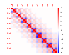
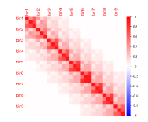
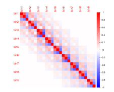
Figure 2: The correlation matrix for parameters in order of {$\alpha_{\parallel},\alpha_{\perp},f\sigma_{8}$} (left panel), {$D_{\rm A},H,f\sigma_{8}$} (middle panel), and {$D_{\rm V},F_{\mathrm{AP}},f\sigma_{8}$} (right panel) at nine effective redshifts.

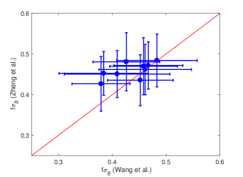
Figure 3: The mean and 68% CL uncertainty of $f\sigma_{8}$ derived from this work (y-axis) in comparison with that in Wang et al. (2018b) (x-axis) at nine effective redshifts.

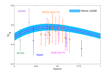
Figure 4: Measurements of $f\sigma_{8}$ in this work (denoted as ‘BOSS 9$z$bin PS’) in comparison with those derived from the Planck data (deep and light blue bands indicating the 68 and 95% CL uncertainties respectively) assuming a $\Lambda$CDM cosmology (Planck Collaboration et al., 2016), 2dFGRS (a circle with error bar) (Percival et al., 2004), 6dFGS (a star with error bar) (Beutler et al., 2012), BOSS at three effective redshifts (squares with error bars) (Beutler et al., 2017b) and WiggleZ (diamonds with error bars) (Blake et al., 2011).

We compare our $f\sigma_{8}$ measurement to that derived in Wang et al. (2018b), which applies the same overlapping redshift slicing scheme in configuration space. The comparison shown in Figure 3 demonstrates that our measurement is consistent with that in Wang et al. (2018b) within 68% CL at all redshifts. We also compare our measurement with that in Beutler et al. (2017b), which uses the same galaxy catalogue, but performs the measurement in three redshift slices. For comparison, we compress our measurement into that at three effective redshifts following the method in Wang et al. (2018b), and find an excellent agreement with Beutler et al. (2017b).

Figure 4 overplots our $f\sigma_{8}$ measurement with those derived from redshift surveys including BOSS DR12 (Beutler et al., 2017b), WiggleZ (Blake et al., 2011), 2dFGRS (Percival et al., 2004) and 6dFGS (Beutler et al., 2012). We also show the 68 and 95% CL bands derived from the Planck mission assuming a $\Lambda$CDM model (Planck Collaboration et al., 2016). As illustrated, our measurement enables a reconstruction of $f\sigma_{8}$ with high temporal resolution in the redshift range of $z\in[0.31,0.64]$, which provides key information for gravity tests.

For the ease of cosmological implications, we derive parameters related to physical BAO distances, including $D_{A},H,D_{V}$ and $F_{\rm AP}$, from our measurement of $\alpha_{\perp}$ and $\alpha_{\parallel}$, where

$$Hr_{s} \equiv H^{\rm fid}r^{\rm fid}_{s}/\alpha_{\parallel},$$

$$\frac{D_{A}}{r_{s}} \equiv \alpha_{\perp}\frac{D^{\rm fid}_{A}}{r^{\rm fid}_{s}},$$

$$F_{\rm AP} \equiv \frac{\alpha_{\perp}}{\alpha_{\parallel}}(1+z)D^{\rm fid}_{A}H^{\rm fid}/c,$$

$$\frac{D_{V}}{r_{s}} \equiv \left[\alpha_{\perp}^{2}\alpha_{\parallel}cz(1+z)^{2}D_{A,{\rm fid}}^{2}H^{-1}_{\rm fid}\right]^{1/3}.$$ (9)

We show the result in Table 7.

As our redshift slices overlap to a large extent, the parameters in each redshift slice correlate with those in other redshift slices. To obtain the data correlation matrix for BAO and RSD parameters, we perform joint fits of BAO and RSD parameters in each pair of redshift slices, and assemble. The resultant correlation matrices are shown in Figure 2. As expected, a positive correlation is seen for any given parameter with that in neighbouring redshift slices, and the correlation decays with separation of the slices in redshifts.

Our tomographic BAO and RSD measurement, including the data covariance matrix, is made publicly available .

3.3 A cosmological implication: constraining the $f(R)$ gravity

In this section, we apply our tomographic BAO and RSD measurement to constrain one subset of modified gravity (MG) models, i.e., the $f(R)$ model.

Among various modified gravity models, the $f(R)$ gravity model has attracted much attention due to its simplicity (it is a one-parameter extension of general relativity), and its wide applicability (see De Felice & Tsujikawa 2010 for a review on the $f(R)$ gravity).

Generically, the effect of MG can be parametrised using two time- and scale-dependent functions $\mu(a,k)$ and $\eta(a,k)$, where $a$ and $k$ denote the scale factor and the wavenumber respectively, to modify the Poisson and anisotropic equations in the conformal Newton gauge,

$$k^{2}\Psi = 4\pi Ga^{2}\mu(a,k)\rho\Delta\;,$$

$$\frac{\Phi}{\Psi} = \eta(a,k)\;,$$ (10)

where $\Delta\equiv\rho\delta+3\frac{aH}{k}(\rho+P)v$ denotes the comoving density perturbation.

For general scalar-tensor theories, $\mu(a,k)$ and $\eta(a,k)$ can be parametrised as (Bertschinger & Zukin, 2008),

$$\mu(a,k) = \frac{1+\beta_{1}\lambda_{1}^{2}k^{2}a^{s}}{1+\lambda_{1}^{2}k^{2}a^{s}},$$

$$\eta(a,k) = \frac{1+\beta_{2}\lambda_{2}^{2}k^{2}a^{s}}{1+\lambda_{2}^{2}k^{2}a^{s}},$$ (11)

where $\beta_{1}$ and $\beta_{2}$ (denoting the coupling; dimensionless), $s$ (the power index; dimensionless), $\lambda_{1}$ and $\lambda_{2}$ (the length scales; in unit of Mpc) are free parameters. $a$ represents the scale factor. In $f(R)$ theory, which is a special case of the scalar-tensor theory, the following relations hold,

$$\beta_{1}=4/3;\ \ \ \beta_{2}=1/2;\ \ \ \lambda_{2}^{2}/\lambda_{1}^{2}=4/3.$$ (12)

In addition, we fix $s=4$ to closely mimic the $\Lambda$CDM model at the background level (Giannantonio et al., 2010; Mueller et al., 2018). This only leaves one free parameter, $\lambda_{1}$, to be determined. In practice, we vary ${\rm log}_{10}B_{0}$ with other cosmological parameters where,

$$B_{0}\equiv\frac{2H_{0}^{2}\lambda_{1}^{2}}{c^{2}}.$$ (13)

The Hubble constant $H_{0}$ and the speed of light $c$ in the equation above make $B_{0}$ dimensionless, and the $\Lambda$CDM limit corresponds to $B_{0}=0$.

To constrain ${\rm log}_{10}B_{0}$, we use three different BAO and RSD measurements derived from the same DR12 combined galaxy sample, combined with the Planck 2015 observations (Planck Collaboration et al., 2016), namely,

• The consensus BAO and RSD measurement reported in Alam et al. (2017);

• The tomographic BAO and RSD measurement in configuration space (Wang et al., 2018b);

• This work.

We use MGCAMB (Zhao et al., 2009; Hojjati et al., 2011) and CosmoMC for parameter estimation, and show the 68 and 95% CL contour plot between ${\rm log}_{10}B_{0}$ and $\Omega_{\rm M}$ in Figure 5. As shown, the contours derived from ‘Planck + Wang’ and ‘Planck + Zheng’ (this work) are consistent with each other at 68% CL, which is expected given the consistency between the BAO and RSD measurement in this work and that in Wang et al. (2018b) (see Figure 3). More importantly, the constraint on ${\rm log}_{10}B_{0}$ derived from ‘Planck + Alam’ is much looser than that derived from ‘Planck + Wang’ or ‘Planck + Zheng’, namely,

$${\rm log}_{10}B_{0}<-4.28\ ({\rm Planck+Alam})$$

$${\rm log}_{10}B_{0}<-4.76\ ({\rm Planck+Zheng})$$ (14)

where the upper limit is for 95% CL. This means that the tomographic information in ‘Planck + Zheng’ reduces the upper limit of ${\rm log}_{10}B_{0}$ by 11%, which is a nontrivial improvement in the constraint. This is expected, as we know that in $f(R)$ gravity, the enhancement of the growth due to $B_{0}$ varies with redshifts, thus tomographic measurements of the growth rate can help tighten the constraint of $B_{0}$. This demonstrates that our method successfully extracts additional information from the DR12 combined galaxy sample, which is able to tighten the constraint on MG parameters. A study on the observational constraint for a wide range of MG models using our tomographic BAO and RSD measurement with other latest observations is working in progress (Li & Zhao, 2018).

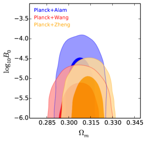
Figure 5: The 68 (inner) and 95% (outer) CL contour plots for log${}_{10}B_{0}$ and $\Omega_{\rm M}$ derived from Planck 15 combined with BAO and RSD measurements at three redshift slices (denoted as ‘Planck+Alam’), Planck 15 combined with BAO and RSD measurements in configuration space at nine redshift slices (denoted as ‘Planck+Wang’), and Planck 15 combined with BAO and RSD measurements in this work (denoted as ‘Planck+Zheng’) respectively.

4 Conclusion and Discussions

With the advance of large galaxy spectroscopic surveys, more and more information on the past light-cone becomes available for cosmological implications. In this work, we apply the overlapping redshift slicing method to the BOSS DR12 combined sample, and perform a joint tomographic BAO and RSD analysis in Fourier space, which largely complements Wang et al. (2018b), the analysis in the configuration space.

Splitting the BOSS DR12 galaxies into nine overlapping redshift slices, we obtain a joint measurement of $D_{A},H$ and $f\sigma_{8}$ with a precision of $2-3\%,\ 3-10\%$ and $9-12\%$, depending on the effective redshifts, respectively. Our measurement covers the redshift range of $0.31<z<0.64$ with a redshift resolution as high as $\Delta z\sim 0.04$. We apply our measurement to constrain the $f(R)$ gravity model for a proof-of-the-concept study, and find that the tomographic information extracted by our method improves the upper limit of the $f(R)$ model parameter ${\rm log_{10}}B_{0}$ by 11%.

Efficient methods for extracting tomographic information from galaxy surveys have been actively developing (Zhao et al., 2017b; Wang et al., 2018b; Wang et al., 2017; Zhu et al., 2015; Zhu et al., 2016; Ruggeri et al., 2017; Ruggeri et al., 2018; Wang et al., 2018a; Zhao et al., 2019; Zhu et al., 2018), which have been proven advantageous for BOSS and eBOSS surveys. More efforts along this line, however, are needed for mitigating theoretical systematics in these methods for example, before making implications on upcoming deeper surveys such as DESI (DESI Collaboration et al., 2016) and PFS (Takada et al., 2014).

References

- Alam et al. (2017) Alam S., et al., 2017, MNRAS, 470, 2617
- Alcock & Paczynski (1979) Alcock C., Paczynski B., 1979, Nature, 281, 358
- Ballinger et al. (1996) Ballinger W. E., Peacock J. A., Heavens A. F., 1996, MNRAS, 282, 877
- Bertschinger & Zukin (2008) Bertschinger E., Zukin P., 2008, Phys. Rev. D, 78, 024015
- Beutler et al. (2012) Beutler F., et al., 2012, MNRAS, 423, 3430
- Beutler et al. (2017a) Beutler F., et al., 2017a, MNRAS, 464, 3409
- Beutler et al. (2017b) Beutler F., et al., 2017b, MNRAS, 466, 2242
- Bianchi et al. (2015) Bianchi D., Gil-Marín H., Ruggeri R., Percival W. J., 2015, MNRAS, 453, L11
- Blake et al. (2011) Blake C., et al., 2011, MNRAS, 415, 2876
- Bolton et al. (2012) Bolton A. S., et al., 2012, AJ, 144, 144
- Chan et al. (2012) Chan K. C., Scoccimarro R., Sheth R. K., 2012, Phys. Rev. D, 85, 083509
- DESI Collaboration et al. (2016) DESI Collaboration et al., 2016, preprint, (ArXiv e-print: 1611.00036)
- De Felice & Tsujikawa (2010) De Felice A., Tsujikawa S., 2010, Living Reviews in Relativity, 13, 3
- Fukugita et al. (1996) Fukugita M., Ichikawa T., Gunn J. E., Doi M., Shimasaku K., Schneider D. P., 1996, AJ, 111, 1748
- Giannantonio et al. (2010) Giannantonio T., Martinelli M., Silvestri A., Melchiorri A., 2010, J. Cosmology Astropart. Phys, 4, 030
- Gil-Marín et al. (2018) Gil-Marín H., et al., 2018, MNRAS, 477, 1604
- Gunn et al. (2006) Gunn J. E., et al., 2006, AJ, 131, 2332
- Hamilton (2000a) Hamilton A. J. S., 2000a, MNRAS, 312, 257
- Hamilton (2000b) Hamilton A. J. S., 2000b, MNRAS, 312, 257
- Hojjati et al. (2011) Hojjati A., Pogosian L., Zhao G.-B., 2011, J. Cosmology Astropart. Phys, 8, 5
- Jing (2005) Jing Y. P., 2005, ApJ, 620, 559
- Kaiser (1987) Kaiser N., 1987, MNRAS, 227, 1
- Kitaura et al. (2016) Kitaura F.-S., et al., 2016, MNRAS, 456, 4156
- Koyama (2016) Koyama K., 2016, Reports on Progress in Physics, 79, 046902
- Leauthaud et al. (2016) Leauthaud A., et al., 2016, MNRAS, 457, 4021
- Lewis & Bridle (2002) Lewis A., Bridle S., 2002, Phys. Rev. D, 66, 103511
- Lewis et al. (2000) Lewis A., Challinor A., Lasenby A., 2000, ApJ, 538, 473
- Li & Zhao (2018) Li J., Zhao G.-B., 2018, preprint, (arXiv:1806.05022)
- Mueller et al. (2018) Mueller E.-M., Percival W., Linder E., Alam S., Zhao G.-B., Sánchez A. G., Beutler F., Brinkmann J., 2018, MNRAS, 475, 2122
- Peebles & Yu (1970) Peebles P. J. E., Yu J. T., 1970, ApJ, 162, 815
- Percival et al. (2004) Percival W. J., et al., 2004, MNRAS, 353, 1201
- Percival et al. (2014) Percival W. J., et al., 2014, MNRAS, 439, 2531
- Perlmutter et al. (1999) Perlmutter S., et al., 1999, ApJ, 517, 565
- Planck Collaboration et al. (2016) Planck Collaboration et al., 2016, A&A, 594, A13
- Reid et al. (2016) Reid B., et al., 2016, MNRAS, 455, 1553
- Riess et al. (1998) Riess A. G., et al., 1998, AJ, 116, 1009
- Rodríguez-Torres et al. (2016) Rodríguez-Torres S. A., et al., 2016, MNRAS, 460, 1173
- Ross et al. (2011) Ross A. J., et al., 2011, MNRAS, 417, 1350
- Ruggeri et al. (2017) Ruggeri R., Percival W. J., Gil-Marín H., Zhu F., Zhao G.-B., Wang Y., 2017, MNRAS, 464, 2698
- Ruggeri et al. (2018) Ruggeri R., et al., 2018, preprint, (arXiv:1801.02891)
- Saito et al. (2016) Saito S., et al., 2016, MNRAS, 460, 1457
- Smee et al. (2013) Smee S. A., et al., 2013, AJ, 146, 32
- Takada et al. (2014) Takada M., et al., 2014, PASJ, 66, R1
- Taruya et al. (2010) Taruya A., Nishimichi T., Saito S., 2010, Phys. Rev. D, 82, 063522
- Taruya et al. (2012) Taruya A., Bernardeau F., Nishimichi T., Codis S., 2012, Phys. Rev. D, 86, 103528
- Wang et al. (2017) Wang Y., et al., 2017, MNRAS, 469, 3762
- Wang et al. (2018a) Wang D., et al., 2018a, MNRAS, 477, 1528
- Wang et al. (2018b) Wang Y., Zhao G.-B., Chuang C.-H., Pellejero-Ibanez M., Zhao C., Kitaura F.-S., Rodriguez-Torres S., 2018b, MNRAS, 481, 3160
- Weinberg et al. (2013) Weinberg D. H., Mortonson M. J., Eisenstein D. J., Hirata C., Riess A. G., Rozo E., 2013, Phys. Rep., 530, 87
- Wilson et al. (2015) Wilson M. J., Peacock J. A., Taylor A. N., de la Torre S., 2015, preprint, (arXiv:1511.07799)
- Wilson et al. (2017) Wilson M. J., Peacock J. A., Taylor A. N., de la Torre S., 2017, MNRAS, 464, 3121
- Zhao et al. (2009) Zhao G.-B., Pogosian L., Silvestri A., Zylberberg J., 2009, Phys. Rev. D, 79, 083513
- Zhao et al. (2017a) Zhao G.-B., et al., 2017a, Nature Astronomy, 1, 627
- Zhao et al. (2017b) Zhao G.-B., et al., 2017b, MNRAS, 466, 762
- Zhao et al. (2019) Zhao G.-B., et al., 2019, MNRAS, 482, 3497
- Zhu et al. (2015) Zhu F., Padmanabhan N., White M., 2015, MNRAS, 451, 236
- Zhu et al. (2016) Zhu F., Padmanabhan N., White M., Ross A. J., Zhao G.-B., 2016, MNRAS, 461, 2867
- Zhu et al. (2018) Zhu F., et al., 2018, MNRAS, 480, 1096