Heavy Flavor Azimuthal Correlations in Cold Nuclear Matter

Abstract

Background: It has been proposed that the azimuthal distributions of heavy flavor quark-antiquark pairs may be modified in the medium of a heavy-ion collision. Purpose: This work tests this proposition through next-to-leading order (NLO) calculations of the azimuthal distribution, $d\sigma/d\phi$, including transverse momentum broadening, employing $\langle k_{T}^{2}\rangle$ and fragmentation in exclusive $Q\overline{Q}$ pair production. While these studies were done for $p+p$, $p+\overline{p}$ and $p+$Pb collisions, understanding azimuthal angle correlations between heavy quarks in these smaller, colder systems is important for their interpretation in heavy-ion collisions. Methods: First, single inclusive $p_{T}$ distributions calculated with the exclusive HVQMNR code are compared to those calculated in the fixed-order next-to-leading logarithm approach. Next the azimuthal distributions are calculated and sensitivities to $\langle k_{T}^{2}\rangle$, $p_{T}$ cut, and rapidity are studied at $\sqrt{s}=7$ TeV. Finally, calculations are compared to $Q\overline{Q}$ data in elementary $p+p$ and $p+\overline{p}$ collisions at $\sqrt{s}=7$ TeV and 1.96 TeV as well as to the nuclear modification factor $R_{p{\rm Pb}}(p_{T})$ in $p+$Pb collisions at $\sqrt{s_{NN}}=5.02$ TeV measured by ALICE. Results: The low $p_{T}$ ($p_{T}<10$ GeV) azimuthal distributions are very sensitive to the $k_{T}$ broadening and rather insensitive to the fragmentation function. The NLO contributions can result in an enhancement at $\phi\sim 0$ absent any other effects. Agreement with the data was found to be good. Conclusions: The NLO calculations, assuming collinear factorization and introducing $k_{T}$ broadening, result in significant modifications of the azimuthal distribution at low $p_{T}$ which must be taken into account in calculations of these distributions in heavy-ion collisions.

I Introduction

Recently there has been interest in heavy flavor correlations and how they might be modified in heavy-ion collisions Andre ; mischke ; gossiaux . However, before drawing any conclusions, it is worth studying these correlations in $p+p$ collisions and how they may be affected in cold nuclear matter. This paper focuses on heavy quark pair correlations in azimuthal angle.

Heavy flavor correlations were previously studied at high $p_{T}$ and high pair invariant mass where they contribute to the background for $Z^{0}$ boson decays Camelia . They were also studied in more elementary collisions, including the effects of final-state radiation in event generators Vermunt and in the $k_{T}$-factorization approach Szczurek .

Correlated production, specifically of the azimuthal angle between heavy flavors, $\phi$, either by direct reconstruction of both $D$ mesons or of a $D$ meson and the decay product of its partner, either a light hadron or a lepton Andre , is a stronger test of $Q\overline{Q}$ production than single inclusive distributions. Naively, at LO $Q\overline{Q}$ pairs are produced back-to-back with a peak at $\phi=\pi$. Higher order production will, however, result in a more isotropic distribution in $\phi$ due to light parton emission in the final state.

Single inclusive heavy flavor production is discussed and compared with data in Sec. II. Because it is not possible to study pair correlations with current approaches to single inclusive distributions such as FONLL FONLL and GV-VFNS GM-VFN , the exclusive HVQMNR NLO code MNRcode is employed to calculate the azimuthal correlations. By modifying the fragmentation function and the intrinsic transverse momentum broadening in the HVQMNR code, it is possible to reproduce the shape of the single heavy flavor transverse momentum distributions from codes like FONLL. This gives confidence in the approach to the calculation of the pair distributions. In this section, methods of calculating exclusive $Q\overline{Q}$ pair production are briefly introduced and a comparison of the next-to-leading order calculation with $Q\overline{Q}$ production in leading event generators is discussed.

After demonstrating that the calculational approaches give reasonably equivalent results, the sensitivity of the azimuthal distributions to the heavy flavor fragmentation function and the intrinsic transverse momentum, $k_{T}$, is explored. Sensitivities to the heavy quark transverse momentum cut, the rapidity range probed, and the renormalization and factorization scales are also discussed in Sec. III. Section IV describes the sensitivity of the azimuthal distributions to the size of $\langle k_{T}^{2}\rangle$, independent of the fragmentation function.

The results are compared to $Q\overline{Q}$ data from $p+p$ and $p+\overline{p}$ collisions in Sec. V and to ALICE $R_{p{\rm Pb}}(p_{T})$ single $D$ meson data from $p+$Pb collisions at $\sqrt{s_{{}_{NN}}}=5.02$ TeV in Sec. VI. In Sec. VI, predictions for cold matter effects on the $\phi$ distribution are also shown.

II Heavy flavor production

II.1 Single inclusive production approaches

There are currently two approaches to heavy flavor production at colliders: collinear factorization and the $k_{T}$-factorization approach, usually employed at low $x$.

There are two main methods of calculating the spectrum of single inclusive open heavy flavor production in perturbative QCD assuming collinear factorization. The underlying idea is similar but the technical approach differs. Both seek to cure the large logarithms of $p_{T}/m$ arising at all orders of the perturbative expansion which can spoil the convergence. The first terms in the expansion are the leading (LL) and next-to-leading logarithmic (NLL) terms, $\alpha_{s}^{2}[\alpha_{s}\log(p_{T}/m)]^{k}$ and $\alpha_{s}^{3}[\alpha_{s}\log(p_{T}/m)]^{k}$ respectively.

It is worth noting that the single inclusive heavy flavor $p_{T}$ distribution is finite at leading order (LO) as $p_{T}\rightarrow 0$ because of the finite quark mass scale. This is in contrast to light hadron and jet production where there is no mass scale to regulate the low $p_{T}$ cross section.

While large uncertainties can arise at low $p_{T}$, these are due to the choice of factorization scale and are larger for charm than for bottom quark production Joszo ; NVF . A next-to-leading order (NLO) calculation that assumes production of massive quarks but neglects LL terms, a “massive” formalism, can result in large uncertainties at high $p_{T}$ FFN-NDE1 ; FFN-NDE2 ; FFN-BKvNS ; FFN-BvNMSS . (This massive formalism is sometimes referred to as a fixed-flavor-number (FFN) scheme.) If, instead, the heavy quark is treated as “massless” and the LL and NLL corrections are absorbed into the fragmentation functions, the approach breaks down as $p_{T}$ approaches $m$ even though it improves the result at high $p_{T}$. The massless formalism is sometimes referred to as the zero-mass, variable-flavor-number (ZM-VFN) scheme ZM-VFN1 ; ZM-VFN2 . There are methods to interpolate smoothly between the FO/FFN scheme at low $p_{T}$ and the massless/ZM-VFN scheme at high $p_{T}$.

The fixed-order next-to-leading logarithm (FONLL) approach is one such method. In FONLL, the fixed order and fragmentation function approaches are merged so that the mass effects are included in an exact calculation of the leading ($\alpha_{s}^{2}$) and next-to-leading ($\alpha_{s}^{3}$) order cross section while also including the LL and NLL terms FONLL . The NLO fixed order (FO) result is combined with a calculation of the resumed (RS) cross section in the massless limit. The FO and RS approaches need to be calculated in the same renormalization scheme with the same number of light flavors. The FONLL result is then, schematically,

$${\rm FONLL}\,=\,{\rm FO}\,+\,({\rm RS}\,-\,{\rm FOM0})G(m,p_{T})\,\,$$ (1)

where FOM0 is the fixed order result at zero mass. The interpolating function $G(m,p_{T})\sim p_{T}^{2}/(p_{T}^{2}+(cm)^{2})$ is arbitrary but must approach unity for $m/p_{T}\rightarrow 0$. Note that the number of light flavors is thus 4 for charm and 5 for bottom quark production in FONLL, in contrast the 3 for charm and 4 for bottom in the fixed-order calculation.

The second interpolation scheme is the generalized-mass variable-flavor-number (GM-VFN) scheme GM-VFN . The large logarithms in charm production for $p_{T}\gg m$ are absorbed in the charm parton distribution function and are thus included in the evolution equations for the parton distributions. The logarithmic terms can be incorporated into the hard cross section to achieve better accuracy for $p_{T}\geq m$. By adjusting the mass-dependent subtraction terms, no interpolating function is required GM-VFN .

In the $k_{T}$-factorization approach, off-shell leading order matrix elements for $g^{*}g^{*}\rightarrow c\overline{c}$ are used together with unintegrated gluon densities that depend on the transverse momentum of the gluon, $k_{T}$, as well as the usual dependence on $x$ and $\mu_{F}$. The motivation for choosing the $k_{T}$-factorized approach is that, at sufficiently low $x$, collinear factorization should no longer hold.

The LHC data has been compared to calculations in both approaches and those assuming collinear factorization compare well with the LHC data. Recent ALICE data ALICEDmesonsNew , at $0<p_{T}<2$ GeV supports collinear factorization. Their $D^{0}$ results at 7 TeV for $|y|<0.5$, were compared to FONLL, GV-VFNS and LO $k_{T}$-factorization calculations. Only the $k_{T}$-factorized calculation is inconsistent with the shape of the data in the $p_{T}$ range where the calculation should best apply. The forward rapidity data of LHCb at 7 TeV LHCbDmesons and 13 TeV Aaij:2015bpa , also agree well with the collinear factorization assumption. The recent 13 TeV data from LHCb is within the uncertainty bands of FONLL and POWHEG (discussed below) down to $p_{T}\rightarrow 0$, albeit with large uncertainty bands and near the upper limit of the calculated band. The GM-VFNS calculation is given only for $p_{T}>3$ GeV but agrees well with the data with small uncertainties Aaij:2015bpa . Perhaps a NLO $k_{T}$-factorized result could lead to improved agreement with the data but, so far, collinear factorization appears to still work well for low $x$, moderate $p_{T}$ charm production.

This paper will thus employ the collinear factorization approach in the calculations.

II.2 Exclusive approaches to heavy flavor production

Recall that the FONLL and GM-VFNS calculations are for single inclusive production only and can thus not address $Q\overline{Q}$ pair observables. There are NLO heavy flavor codes that, in addition to inclusive heavy flavor production, also calculate exclusive $Q\overline{Q}$ pair production.

The HVQMNR code MNRcode uses negative weight events to cancel divergences numerically. Smearing the parton momentum through the introduction of intrinsic transverse momenta, $k_{T}$, reduces the importance of the negative weight events at low $p_{T}$. HVQMNR does not include any resummation.

POWHEG-hvq POWHEG is a positive weight generator that includes leading-log resummation. The entire event is available since PYTHIA PYTHIA and HERWIG HERWIG are employed to produce the complete event after production of the $Q\overline{Q}$ pair.

The $k_{T}$-factorization approach can also be employed to calculate correlated $c\overline{c}$ production since the unintegrated parton densities have a transverse component, giving finite $p_{T}$ and $\phi$ distributions even at LO Szczurek .

The HVQMNR code is employed here to focus on the effects due to the NLO contribution alone, including $k_{T}$-broadening and fragmentation but excluding the parton showers which can further randomize the pair momenta and thus affect the angular correlations.

II.3 Heavy flavor production in leading order event generators compared to NLO calculations

In addition to these NLO codes, heavy flavor correlations can also be simulated employing LO event generators such as PYTHIA.

In an event generator like PYTHIA or HERWIG, heavy flavor production is divided into three different categories: flavor or pair creation, flavor excitation, and gluon splitting Bedjidian:2004gd . This classification depends on the number of heavy quarks in the final state of the hard process, defined as the process in the event with the highest virtuality. Pair creation is equivalent to the four leading order diagrams, shown in Fig. 1. In this case the final state has two heavy quarks, the $Q$ and $\overline{Q}$. In the case of flavor excitation, a heavy quark from the splitting $g\rightarrow Q\overline{Q}$ in an initial-state parton shower is put on mass shell by scattering with a parton, either a quark or gluon, from the other beam, $qQ\rightarrow qQ$ or $gQ\rightarrow gQ$. There is thus one heavy quark in the final state of the hard scattering. Finally, gluon splitting is defined as having no heavy flavor in the hard scattering such as $gg\rightarrow gg$. The $Q\overline{Q}$ pair is produced in an initial- or final-state parton shower via $g\rightarrow Q\overline{Q}$. Double counting of these processes is avoided by requiring that the hard scattering should be of greater virtuality than the parton shower Bedjidian:2004gd .

Figure 1: Leading order $Q\overline{Q}$ production diagrams with (a) the $q\overline{q}$ initial state and (b)-(d) the $gg$ contributions.

There are parameters that can be tuned, depending on the generator employed, that can match the distributions from the LO generator to those of a NLO calculation. However, that does not mean that the mix of physics processes is identical. For example, all three of the $Q\overline{Q}$ production processes in PYTHIA contribute to perturbative QCD production at next-to-leading order with $2\rightarrow 3$ processes. Pair creation is realized at NLO by gluon emission from one of the final-state heavy quarks, as in Fig. 2(a), the NLO version of Fig. 1(c). Flavor excitation off a gluon from the opposite hadron is shown in Fig. 2(b) while gluon splitting is shown in Fig. 2(c).

Figure 2: Examples of real contributions to next-to-leading order $Q\overline{Q}$ production. Diagrams (a)-(c) illustrate contributions to $gg\rightarrow Q\overline{Q}g$ while (d) shows an example of $qg\rightarrow qQ\overline{Q}$ production.

The diagrams in Fig. 2(a)-(c) are an illustration of the possible NLO diagrams included in $gg$-initiated $Q\overline{Q}$ production, $gg\rightarrow Q\overline{Q}g$. For example, virtual corrections and crossed diagrams are not shown in Fig. 2. In a NLO calculation, the amplitudes from these $gg$ contributions are summed with weights determined by the spin and color factors of each diagram, not parton showers and individual virtualities. Instead, production processes are separated by the initial state. The $gg$ initial state is dominant at collider energies over most of the rapidity range. The next largest contribution is due to $qg$ or $\overline{q}g$ scattering, $qg\rightarrow qQ\overline{Q}$, shown in Fig. 2(d), and not present at leading order. This diagram is considered to be flavor excitation in event generators. Finally, real and virtual corrections in the $q\overline{q}$ channel, $q\overline{q}\rightarrow Q\overline{Q}g$, makes a small contribution to $Q\overline{Q}$ production at high energies.

Due to the common use of event generators in simulations and analysis, there is a great temptation to try and analyze heavy flavor production in terms of separate production mechanisms, as characterized by creation, excitation and splitting. However, as described here, there is no distinction, all three are components of NLO production. Separating the diagrams in the initial $gg$ process in such a manner will result in improper interferences in the calculation and an incorrect cross section. Thus it is preferable to do these types of analyses with an exclusive NLO code such as described in Sec. II.2.

II.4 $k_{T}$ broadening and fragmentation

The transition from bare quark distributions to those of the final-state hadrons is accomplished by including a fragmentation function and intrinsic transverse momentum, $k_{T}$, broadening. The implementation of these two effects are described here.

II.4.1 Intrinsic $k_{T}$ broadening

Results on open heavy flavors at fixed-target energies indicated that some level of transverse momentum broadening was needed to obtain agreement with the low $p_{T}$ data after fragmentation was applied MLM1 . Broadening is typically applied by including some intrinsic transverse momentum, $k_{T}$, smearing to the initial-state parton densities. The implementation of intrinsic $k_{T}$ in HVQMNR is not handled in the same way as calculations of other hard processes due to the nature of the code. In HVQMNR, the cancellation of divergences is done numerically. Since adding further numerical Monte-Carlo integrations would slow the simulation of events, as well as require multiple runs in the same kinematics but with different intrinsic $k_{T}$ kicks, the kick is added in the final, rather than the initial, state. The Gaussian function $g_{p}(k_{T})$ MLM1 ,

$$g_{p}(k_{T})=\frac{1}{\pi\langle k_{T}^{2}\rangle}\exp(-k_{T}^{2}/\langle k_{T}^{2}\rangle)\,\,,$$ (2)

multiplies the parton distribution functions for both hadrons, assuming the $x$ and $k_{T}$ dependencies in the initial partons completely factorize. If factorization applies, it does not matter whether the $k_{T}$ dependence appears in the initial or final state as long as the kick is not too large. In Ref. MLM1 , $\langle k_{T}^{2}\rangle=1$ GeV² was chosen to describe the $p_{T}$ dependence of fixed-target charm production.

In HVQMNR, the $Q\overline{Q}$ system is boosted to the rest frame from its longitudinal center-of-mass frame. Intrinsic transverse momenta of the incoming partons, $\vec{k}_{T1}$ and $\vec{k}_{T2}$, are chosen at random with $k_{T1}^{2}$ and $k_{T2}^{2}$ distributed according to Eq. (2). A second transverse boost out of the pair rest frame changes the initial transverse momentum of the $Q\overline{Q}$ pair, $\vec{p}_{T}$, to $\vec{p}_{T}+\vec{k}_{T1}+\vec{k}_{T2}$. The initial $k_{T}$ of the partons could have alternatively been given to the entire final-state system, as is essentially done if applied in the initial state, instead of to the $Q\overline{Q}$ pair. There is no difference if the calculation is LO but at NLO an additional light parton can also appear in the final state, making the correspondence inexact. In Ref. MLM1 , the difference between the two implementations is claimed to be small if $\langle k_{T}^{2}\rangle\leq 2$ GeV². The $p_{T}$-integrated rapidity distribution is unaffected by the intrinsic $k_{T}$.

The level of the intrinsic $k_{T}$ kick required in these calculations was determined by comparison with the shape of the quarkonium $p_{T}$ distributions. In this case, the Color Evaporation Model is employed to calculate production with a cut on the pair invariant mass in the HVQMNR code, giving an upper limit of $2m_{H}$ where $H=D$, $B$ for charm and bottom respectively. The CEM pair distributions require augmentation by $k_{T}$ broadening to make them finite at $p_{T}\rightarrow 0$, as do the $Q\overline{Q}$ pair $p_{T}$ distributions. The $k_{T}$ broadening has the most important effect on the azimuthal correlation at low $p_{T}$ as well, as we will show.

The effect of the $k_{T}$ kick on the $p_{T}$ distribution can be expected to decrease as $\sqrt{s}$ increases because the average $p_{T}$ also increases with energy. However, the value of $\langle k_{T}^{2}\rangle$ is assumed to increase with $\sqrt{s}$ so that effect remains important for low $p_{T}$ production at higher energies. The energy dependence of $\langle k_{T}^{2}\rangle$ in Ref. NVF is

$$\langle k_{T}^{2}\rangle=1+\frac{1}{n}\ln\left(\frac{\sqrt{s}}{20\,{\rm GeV}}\right)\,\,{\rm GeV}^{2}\,\,.$$ (3)

Comparison with the RHIC $J/\psi$ data found that $n=12$ gave the best description of the $J/\psi$ $p_{T}$ distribution both at central and forward rapidity NVF . The value of $n$ was unchanged in the Improved Color Evaporation Model MaVogt . A smaller value of $n$ and thus a larger $\langle k_{T}^{2}\rangle$ is required for the $\Upsilon$ $p_{T}$ distribution. For $\Upsilon$, $n=3$ is set by comparison to the Tevatron results at $\sqrt{s}=1.8$ TeV NVFinprep . These same values are also used in the charm and bottom pair distributions.

II.4.2 Fragmentation

The default fragmentation function in HVQMNR is the Peterson function Pete ,

$$D(z)=\frac{z(1-z)^{2}}{((1-z)^{2}+z\epsilon_{P})^{2}}\,\,,$$ (4)

where $z$ represents the fraction of the parent heavy flavor quark momentum carried by the resulting heavy flavor hadron. In the original Peterson function, the nominal values of the fragmentation parameter $\epsilon_{P}$ were 0.06 for charm and 0.006 for bottom. These values result in $\langle z\rangle=0.671$ for charm and 0.828 for bottom, a reduction in the heavy quark momentum of $\sim 33$% and 17% respectively, as shown by the red curves in Fig. 3. Currently, the Peterson function with $\epsilon_{P}=0.06$ is considered too strong for charm production. The FONLL fragmentation scheme for open heavy flavor is softer CNV , as will be discussed.

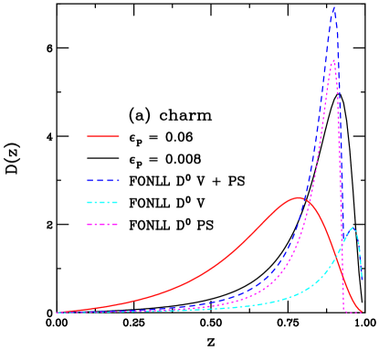
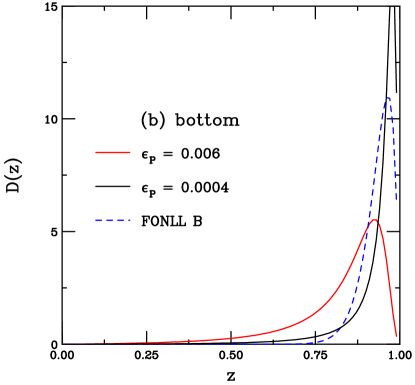
Figure 3: (Color online) The fragmentation functions used in the HVQMNR code and FONLL for (a) charm and (b) bottom are compared. The red curves show the standard Peterson function parameter while the black curves are calculated with the values of $\epsilon_{P}$ used in this paper. The FONLL results are shown in the dashed blue curves. For charm quarks, the total FONLL contribution to $D^{0}$ fragmentation includes the vector (V) and pseudoscalar (PS) contributions, shown separately.

The value of $\epsilon_{P}$ in the Peterson fragmentation function must be modified to match the FONLL $p_{T}$ distribution for single $D$ and $B$ meson production since the standard $\epsilon_{P}$ values for Eq. (4) result in much softer $p_{T}$ distributions than those of FONLL. Therefore, the value of $\epsilon_{P}$ needs to be reduced to match the average ratio of the heavy quark momentum transferred to the final state hadron, $\langle z\rangle$. The average $z$ is calculated as

$$\langle z\rangle=\frac{\int_{0}^{1}dzzD(z)}{\int_{0}^{1}dzD(z)}\,\,.$$ (5)

Fragmentation functions for $D$ and $D^{*}$ mesons have been calculated in an approach consistent with an FONLL calculation CN_CDF . The FONLL charm fragmentation function was determined from Mellin moments of the distributions calculated consistently in the same framework. The $D^{0}$ fragmentation function includes both pseudoscalar and vector parts that account for the ground state, $c\rightarrow D^{0}$, and excited state contributions, $c\rightarrow D^{*0}\rightarrow D^{0}$ and $c\rightarrow D^{*+}\rightarrow D^{0}$ respectively. The fragmentation parameter for $D^{0}$ with a central charm quark mass of $m=1.5$ GeV CNV was adjusted to the chosen central value of the charm quark mass, 1.27 GeV, used here. Assuming a linear dependence of $\epsilon_{P}$ on charm mass from 1.2 to 1.7 GeV, the total FONLL charm fragmentation function is given by the blue dashed curve in Fig. 3(a). The vector and pseudoscalar contributions are shown in the cyan and magenta curves respectively. Individually, their average $z$ values are $\langle z\rangle=0.812$ for the pseudoscalar channel and 0.843 for the more massive $D^{*}$ in the vector channel. Note that the vector channel is a small overall contribution to the combined fragmentation function, as is reflected in the average $z$ for the total FONLL fragmentation function, 0.822. This $\langle z\rangle$ can be compared to the result obtained with the default value of $\epsilon_{P}$ in the Peterson function, $\langle z\rangle=0.671$. The calculations in this work will use the reduced value, $\epsilon_{P}=0.008$, shown in the black curve in Fig. 3(a). Using this $\epsilon_{P}$, $\langle z\rangle=0.820$, in good agreement with the average $z$ for the combined FONLL charm fragmentation function. As will be shown in Sec. II.5, the single inclusive $D$ meson $p_{T}$ distribution calculated with HVQMNR for this $\epsilon_{P}$, combined with the value of $\langle k_{T}^{2}\rangle$ determined from RHIC with the energy dependence of Eq. (3), is in good agreement with the FONLL $p_{T}$ distribution.

The bottom quark fragmentation function in FONLL is of the form

$$D(z)=z(1-z)^{\epsilon_{b}}$$ (6)

where $\epsilon_{b}=34$ for a bottom quark mass of 4.75 GeV CNV . Again, assuming a linear dependence of $\epsilon_{b}$ on $b$ quark mass from 4.5 to 5 GeV, with $m_{b}=4.65$ GeV, $\epsilon_{b}=27.5$. The FONLL fragmentation function with this value of $\epsilon_{b}$, is shown in the dashed blue curve of Fig. 3(b). In this case, $\langle z\rangle=0.934$. In contrast, the red curve shows the default Peterson function result for $\epsilon_{P}=0.006$, with $\langle z\rangle=0.828$. If the same overall reduction of the Peterson function parameter for charm is used for bottom, from 0.006 to 0.0008, $\langle z\rangle=0.911$, insufficient to replicate the FONLL $B$ meson $p_{T}$ dependence. Thus, $\epsilon_{P}=0.0004$ is used here, giving $\langle z\rangle=0.930$, in good agreement with the average $z$ from FONLL, as shown in the solid black curve of Fig. 3(b).

The charm and bottom $p_{T}$ distributions employing these fragmentation functions will be compared to those from FONLL in the next section.

II.5 Single Inclusive Heavy Flavor Distributions

In the calculations reported in this paper, the same values of the charm quark mass and scale parameters as in Ref. NVF are employed here, $(m,\mu_{F}/m_{T},\mu_{R}/m_{T})=(1.27\pm 0.09\,{\rm GeV},2.1^{+2.55}_{-0.85},1.6^{+0.11}_{-0.12})$ where $\mu_{F}$ is the factorization scale and $\mu_{R}$ is the renormalization scale. In the case of bottom production, $(m,\mu_{F}/m_{T},\mu_{R}/m_{T})=(4.65\pm 0.09\,{\rm GeV},1.4^{+0.77}_{-0.49},1.1^{+0.22}_{-0.20})$ is used NVFinprep . The CT10 proton parton densities CT10 are employed in the calculations. The scale factors, $\mu_{F}$ and $\mu_{R}$, are defined relative to the transverse mass of the pair, $\mu_{F,R}\propto m_{T}=\sqrt{m^{2}+p_{T}^{2}}$ where the $p_{T}$ is the $Q\overline{Q}$ pair $p_{T}$, $p_{T}^{2}=0.5(p_{T_{Q}}^{2}+p_{T_{\overline{Q}}}^{2})$. At LO in the total cross section, the $Q\overline{Q}$ pair $p_{T}$ is zero. Thus, while the calculation is NLO in the total cross section, it is LO in the pair distributions. In the exclusive NLO calculation  MNRcode both the $Q$ and $\overline{Q}$ variables are retained to obtain the pair distributions. Unless otherwise noted, the calculations employ the central values of the heavy quark mass and scale factors.

First, the relative importance of $k_{T}$ broadening and fragmentation on the single inclusive heavy quark $p_{T}$ distribution is studied. Undertaking a study of the azimuthal correlations between heavy quarks requires finding the values of $\langle k_{T}^{2}\rangle$ and $\epsilon_{P}$ appropriate for a reasonably faithful reproduction of the FONLL single inclusive heavy quark distributions in the same kinematics employing the HVQMNR code. These same values of $\langle k_{T}^{2}\rangle$ and $\epsilon_{P}$ are then used in the calculation of the azimuthal distributions. The values of $\langle k_{T}^{2}\rangle$ obtained for $J/\psi$ and $\Upsilon$ production are assumed as a default.

Figure 4 shows how $\langle k_{T}^{2}\rangle$ and $\epsilon_{P}$ affect the low $p_{T}$ part of the spectrum at $\sqrt{s}=7$ TeV. As examples, the charm distributions are shown at forward rapidity, $2.5<y<5$, the LHCb acceptance LHCbDmesons , while the bottom distributions are shown at central rapidity, $|y|<2.4$, the rapidity region of $b$ hadron distributions reported by ATLAS ATLAS_bhad . Note that the lower $p_{T}$ range is emphasized in Fig. 4 because this region is most affected by $k_{T}$ broadening, as discussed in more detail later.

The blue solid curves in Fig. 4 are the bare quark distributions, with $\langle k_{T}^{2}\rangle=0$, $\epsilon_{P}=0$. This distribution is the hardest of all the cases shown and thus has the highest average $p_{T}$. (See Table 1 for the values of $\langle p_{T}\rangle$ with each $\langle k_{T}^{2}\rangle$, $\epsilon_{P}$ combination.)

charm			bottom
$\langle k_{T}^{2}\rangle$	$\epsilon_{p}$	$\langle p_{T}\rangle$	$\langle k_{T}^{2}\rangle$	$\epsilon_{p}$	$\langle p_{T}\rangle$
(GeV2)		(GeV)	(GeV2)		(GeV)
0	0	1.96	0	0	5.38
0	0.06	1.31	0	0.006	4.45
0	0.008	1.58	0	0.0008	4.90
1.5	0.008	1.71	0	0.0004	5.00
3	0.008	1.84	3	0.0004	5.12

Table 1: Average $p_{T}$ for single inclusive charm and bottom quark production for the chosen values of $\langle k_{T}^{2}\rangle$ and $\epsilon_{P}$.

The dashed curves, with the lowest average $p_{T}$, include no broadening but employ the default Peterson fragmentation function parameter from $e^{+}e^{-}$ data Chirin , $\epsilon_{P}=0.06$ for charm and 0.006 for bottom, corresponding to the red curves in Fig. 3. The effect on the charm quark distributions is particularly strong because this value of $\epsilon_{P}$ results in a $\sim 33$% decrease in $p_{T}$ relative to the bare quark, as already discussed. At fixed-target energies, such a strong reduction in momentum could only be made compatible with data, which agreed rather well with the low $p_{T}$ bare charm quark distribution, by setting $\langle k_{T}^{2}\rangle=1$ GeV² MLM1 . For fixed-target energies, $\sqrt{s}\sim 20$ GeV, this was sufficient because the average $p_{T}^{2}$ of the charm quark was low since $m_{c}/\sqrt{s}\sim 0.065$. Therefore, $\langle k_{T}^{2}\rangle\sim\langle p_{T}^{2}\rangle$. However, at collider energies, $m_{c}/\sqrt{s}$ is small, $\sim 1.8\times 10^{-4}$ at $\sqrt{s}=7$ TeV. Thus an average $\langle k_{T}^{2}\rangle$ on the order of $1-3$ GeV² has a rather small effect on the shape of the $p_{T}$ distribution, particularly at high $p_{T}$. On the other hand, $\epsilon_{P}$ reduces the quark $p_{T}$ uniformly, independent of the center-of-mass energy.

The effect of fragmentation on the bottom quark distribution is less striking because $\epsilon_{P}$ is an order of magnitude smaller. Nonetheless, as will be shown in Fig. 5, it is clear that even this milder effect may be too strong to be compatible with the $b$-hadron data.

While $\langle k_{T}^{2}\rangle\sim 1$ GeV² was sufficient to mitigate the effect of fragmentation on charm production at $\sqrt{s}=20$ GeV MLM1 , it is clear that any value of $\langle k_{T}^{2}\rangle$ large enough to do so at $\sqrt{s}=7$ TeV would be too large to be physical. Thus, a reduction of $\epsilon_{P}$ by a factor of $\sim 7.5$, to 0.008 for charm and 0.0008 for bottom, was checked (dot-dashed curves in Fig. 4). This reduction is adequate for charm production, giving a result intermediate to the free quark distribution and that with the standard Peterson fragmentation parameter $\epsilon_{P}$. However, it was found necessary to reduce $\epsilon_{P}$ by an additional factor of two, to 0.0004, for bottom (red solid curve in Fig. 4(b)). This additional reduction is sufficient to produce a $b$-hadron distribution similar to that of FONLL when broadening is included.

Next, the effect of $\langle k_{T}^{2}\rangle$ broadening is introduced in addition to fragmentation. As mentioned previously, the default values of $\langle k_{T}^{2}\rangle$ for charm and bottom are assumed to be those found to agree with low $p_{T}$ quarkonium production in the Improved Color Evaporation Model MaVogt . The energy dependence of $\langle k_{T}^{2}\rangle$ is given in Eq. (3). At $\sqrt{s}=7$ TeV, Eq. (3) results in $\langle k_{T}^{2}\rangle\sim 1.5$ GeV² for charm and $\sim 3$ GeV² for bottom. It is clear that even these relatively large values, although still less than $\langle p_{T}^{2}\rangle$ at $\sqrt{s}=7$ TeV, have a rather small effect on the single inclusive heavy quark $p_{T}$ distribution. Indeed, doubling $\langle k_{T}^{2}\rangle$ for charm (magenta curve in Fig. 4(a)) results in only a small change in the $p_{T}$ distribution in the range shown. No further increase of $\langle k_{T}^{2}\rangle$ is shown for bottom quarks because such values, $\langle k_{T}^{2}\rangle>3$ GeV², would be too large for the assumption of the equivalence of adding $\langle k_{T}^{2}\rangle$ in the initial or final state MLM1 .

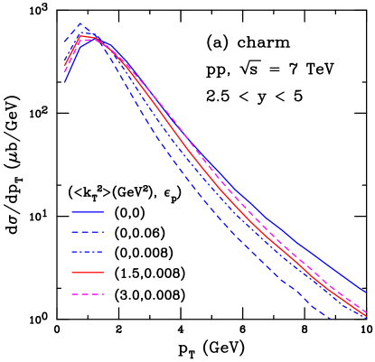
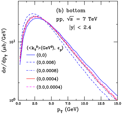
Figure 4: (Color online) The single inclusive (a) charm and (b) bottom quark distributions in $\sqrt{s}=7$ TeV $p+p$ collisions at next-to-leading order using the HVQMNR code. The charm distributions are given at forward rapidity, $2.5<y<5$, while the bottom quark distributions are given at midrapidity, $|y|<2.4$. Results are shown for various combinations of $\langle k_{T}^{2}\rangle$ (Eq. (3)) and $\epsilon_{P}$ (Eq. (4)).

In Fig. 5, the final values of $\langle k_{T}^{2}\rangle$ and $\epsilon_{P}$, $\sim 1.5$ GeV², 0.008 for charm and 3 GeV², 0.0004 for bottom, are used to calculate the uncertainty bands on the HVQMNR results and compare them to those of FONLL, with its default fragmentation functions. The same mass and scale parameters are employed in the HVQMNR and FONLL calculations. The results are compared to LHCb $D^{0}$ meson data in Fig. 5(a), and ATLAS $b$-hadron data in Fig. 5(b). In the HVQMNR calculations, the values of $\langle k_{T}^{2}\rangle$ and $\epsilon_{P}$ are used for all mass and scale choices. In the FONLL calculations, the fragmentation parameter depends on the quark mass but is independent of scale.

The mass and scale uncertainties are calculated based on results using the one standard deviation uncertainties on the quark mass and scale parameters. If the central, upper and lower limits of $\mu_{R,F}/m$ are denoted as $C$, $H$, and $L$ respectively, then the seven sets used to determine the scale uncertainty are $\{(\mu_{F}/m,\mu_{F}/m)\}$ = $\{$$(C,C)$, $(H,H)$, $(L,L)$, $(C,L)$, $(L,C)$, $(C,H)$, $(H,C)$$\}$. The uncertainty band can be obtained for the best fit sets NVF ; NVFinprep by adding the uncertainties from the mass and scale variations in quadrature. The envelope contained by the resulting curves,

$$\frac{d\sigma_{\rm max}}{dX} = \frac{d\sigma_{\rm cent}}{dX}$$

$$\mbox{}\!\!\!\!\!\!\!\!\!\!\!\!\!\!\!\!\!\!\!\!\!\!\!\!\!\!\!\!\!\!+\sqrt{\left(\frac{d\sigma_{\mu,{\rm max}}}{dX}-\frac{d\sigma_{\rm cent}}{dX}\right)^{2}+\left(\frac{d\sigma_{m,{\rm max}}}{dX}-\frac{d\sigma_{\rm cent}}{dX}\right)^{2}}\,\,,$$

$$\frac{d\sigma_{\rm min}}{dX} = \frac{d\sigma_{\rm cent}}{dX}$$

$$\mbox{}\!\!\!\!\!\!\!\!\!\!\!\!\!\!\!\!\!\!\!\!\!\!\!\!\!\!\!\!\!\!-\sqrt{\left(\frac{d\sigma_{\mu,{\rm min}}}{dX}-\frac{d\sigma_{\rm cent}}{dX}\right)^{2}+\left(\frac{d\sigma_{m,{\rm min}}}{dX}-\frac{d\sigma_{\rm cent}}{dX}\right)^{2}}\,\,,$$

defines the uncertainty on the cross section. The kinematic observable $X$ can be e.g. $p_{T}$ or azimuthal angular separation $\phi$. In the calculation labeled “cent”, the central values of $m$, $\mu_{F}$ and $\mu_{R}$ are used while in the calculations with subscript $\mu$, the mass is fixed to the central value while the scales are varied and in the calculations with subscript $m$, the mass is varied while the scales are held fixed.

As an example, Fig. 5(a) compares the calculations in the rapidity interval $2.5<y<3$ to the LHCb $D^{0}$ data LHCbDmesons . The LHCb data in the range $2.5<y<5$ was divided into five rapidity bins, each of 0.5 units of rapidity in width. The lowest of these bins is shown as an example. The agreement between the two calculations is generally very good. Some disagreement becomes apparent for $p_{T}>10$ GeV where the upper limit of the band calculated using the exclusive HVQMNR code becomes slightly harder than the FONLL result, as can be expected because FONLL was designed to cure large logarithms of $p_{T}/m$ and here $p_{T}/m>10$. This region, as will be shown, is also relative insensitive to effects of $\langle k_{T}^{2}\rangle$ on the azimuthal distributions.

There is a somewhat larger difference in the calculations of the $b$-hadron distributions in Fig. 5(b). In this case, the results are shown, along with the ATLAS data ATLAS_bhad , at midrapidity and up to considerably higher $p_{T}$. It is, however, worth noting that, at $p_{T}\sim 50$ GeV, $p_{T}/m$ for bottom is similar to that for charm at $p_{T}\sim 10$ GeV. Here the one standard deviation fit to the $b\overline{b}$ cross section gives a narrower range on $m_{b}$ and $\mu_{F}/m_{T}$, $\mu_{R}/m_{T}$. To improve the agreement between the calculations still further it would be necessary to employ $\epsilon_{P}=0$ in the HVQMNR calculation since the FONLL $b$-hadron $p_{T}$ distribution is equivalent to the HVQMNR bare $b$-quark distribution.

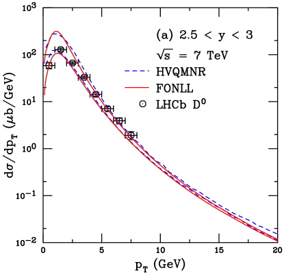
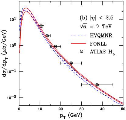
Figure 5: (Color online) The single inclusive (a) $D^{0}$ and (b) $b$-quark hadron, $H_{b}$, distributions in $\sqrt{s}=7$ TeV $p+p$ collisions are compared to data from LHCb LHCbDmesons at $2.5<y<3$ and ATLAS ATLAS_bhad at $|\eta|<2.5$ respectively. The curves show the extent of the uncertainty bands calculated employing Eqs. (II.5) and (II.5). The HVQMNR code (blue dashed curves) utilizes $(\langle k_{T}^{2}\rangle({\rm GeV}^{2}),\epsilon_{P})=(1.5,0.008)$ for charm and (3,0.0004) for bottom. The corresponding FONLL uncertainty band (red curves) is also shown. The same quark mass and scale parameters are used in both calculations.

III $Q\overline{Q}$ Pair Azimuthal Distributions

The single inclusive heavy quark distributions have been calculated both in the exclusive $Q\overline{Q}$ code, HVQMNR, and the inclusive-only FONLL approach and have been shown to agree well with each other. The next step is to calculate the azimuthal angular separation between the two heavy quarks. In Fig. 6, the distributions, $d\sigma/d\phi$, are calculated to next-to-leading order for the same choices of $\langle k_{T}^{2}\rangle$ and $\epsilon_{P}$, with the central mass and scale values, as in Fig. 4, using HVQMNR only since now an exclusive calculation is required to obtain $d\sigma/d\phi$. First, some topological details relevant to the azimuthal distributions of $Q\overline{Q}$ pair production are discussed.

The leading order perturbative QCD $2\rightarrow 2$ diagrams for heavy flavor production, shown in Fig. 1, produce back-to-back $Q\overline{Q}$ pairs with an azimuthal separation of $\phi=\pi$. At leading order, the $p_{T}$ of the pair of heavy quarks is zero and $d\sigma/d\phi$ is represented by a delta function, $\delta(\phi-\pi)$. Note also that, already at leading order, the single inclusive heavy quark $p_{T}$ distribution is maximally hard so that higher order corrections do not significantly change the shape of the $p_{T}$ distribution RVKfact1 ; RVKfact2 .

As discussed in Sec. II.3, at next-to-leading order, both virtual and real conntributions arise. The virtual corrections are typically the exchange of soft gluons at the vertices while real corrections give rise to $2\rightarrow 3$ processes, see Fig. 2. These corrections smear out the azimuthal separation in the leading order contribution so that while there is still a peak at $\phi=\pi$, the pairs are no longer strictly back-to-back. Instead, there is a tail toward $\phi\sim 0$, even with $\langle k_{T}^{2}\rangle=0$ and $\epsilon_{P}=0$.

The NLO contribution can also lead to different azimuthal topologies, as in Fig. 2(b)-(d), due to ‘flavor excitation’ and ‘gluon splitting’. These diagrams do not harden the single inclusive heavy flavor $p_{T}$ distribution. However, they do tend to make the azimuthal correlation more isotropic Bedjidian:2004gd . The $2\rightarrow 3$ processes produce a non-singular azimuthal distribution at $\phi=\pi$ before any broadening or fragmentation is taken into account. A final-state light parton emitted from one of the outgoing heavy quarks is likely to be collinear to the heavy quark that emitted it. Thus the heavy quark and anti-quark remain close to a back-to-back configuration with a peak at $\phi\sim\pi$. However, if the light parton is from the initial state, as in $qg$ scattering, this parton can be hard and its momentum can be balanced against that of the $Q\overline{Q}$ pair so that $\phi\sim 0$. In addition, the ‘gluon splitting’ diagram of Fig. 2(c), will result in a pair with $\phi\sim 0$ against a hard parton. Thus, the low $p_{T}$ heavy quarks azimuthal distribution is likely to be more isotropic, while high $p_{T}$ heavy quarks will more likely result in a doubly-peaked $\phi$ distribution, with peaks at $\phi\sim 0$ and $\pi$.

Fragmentation results in a hadron with momentum nearly collinear to the original heavy quark. Thus fragmentation does not change the general direction of the parent heavy parton. The resulting heavy hadron will, however, be somewhat out of alignment with the initial heavy quark. The larger the value of $\epsilon_{P}$, then, the greater the energy lost to hadronization and the more likely that the $Q$ and $\overline{Q}$ are out of alignment, resulting in a slight enhancement at $\phi\sim 0$ relative to $\epsilon_{P}=0$. Lower values of $\epsilon_{P}$ reduce any enhancement at $\phi\sim 0$, as is evident in the dashed and dot-dashed curves in Fig. 6(a) for $\epsilon_{P}=0.06$ and 0.008 respectively.

On the other hand, including the randomization of the final-state parton momentum by $k_{T}$ broadening has a substantial efect on $d\sigma/d\phi$. Indeed, the level of $k_{T}$ broadening required to describe $J/\psi$ production at low $p_{T}$ completely changes the shape of $d\sigma/d\phi$ for $c\overline{c}$, resulting in a peak at $\phi\sim 0$ and none at $\phi\sim\pi$. The larger value of $\langle k_{T}^{2}\rangle$, $\sim 3$ GeV², increases the enhancement at $\phi\sim 0$, as shown in Fig. 6(a).

In the case of $b\overline{b}$ pairs, introducing $k_{T}$ broadening still gives a peak near $\phi\sim\pi$, even though the $\langle k_{T}^{2}\rangle$ for bottom shown in Fig. 6(b) is as large as the upper value of $\langle k_{T}^{2}\rangle$ for charm in Fig. 6(a). This is because $\langle k_{T}^{2}\rangle\sim 1.5$ GeV² is on the order of $m_{c}^{2}$, $\sim 1.7$ GeV², while $\langle k_{T}^{2}\rangle=3$ GeV² for botttom is considerably less than $m_{b}^{2}\sim 21.6$ GeV². Thus $\langle k_{T}^{2}\rangle/m_{c}^{2}\sim 1$ results in a much more isotropic $\phi$ distribution while $\langle k_{T}^{2}\rangle/m_{b}^{2}\sim 0.14$ results in a lower momentum kick imparted to a bottom quark.

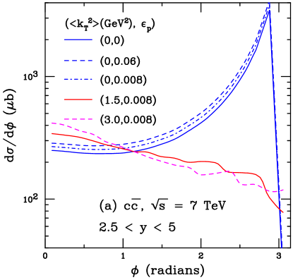
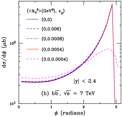
Figure 6: (Color online) The NLO azimuthal distribution between two heavy quarks, $d\sigma/d\phi$ in $p+p$ collisions at $\sqrt{s}=7$ TeV using the HVQMNR code for (a) $c\overline{c}$ pairs at forward rapidity, $2.5<y<5$, and (b) $b\overline{b}$ pairs at midrapidity, $|y|<2.4$. The results are shown for the same combinations of $\langle k_{T}^{2}\rangle$ in Eq. (3) and $\epsilon_{P}$ in Eq. (4) as in Fig. 4.

To illustrate the results more clearly, the ratio of all calculations are shown relative to the results for bare quarks, with $\langle k_{T}^{2}\rangle=0$, $\epsilon_{P}=0$ in Fig. 7. In both cases, the results with only finite $\epsilon_{P}$ and $\langle k_{T}^{2}\rangle=0$ are relatively independent of $\phi$ with the largest values of $(d\sigma(\langle k_{T}^{2}\rangle,\epsilon_{P})/d\phi)/(d\sigma(\langle k_{T}^{2}\rangle=0,\epsilon_{P}=0)/d\phi)$ for the default values of $\epsilon_{P}$, 0.06 for charm and 0.006 for bottom. For charm production, the ratio is $\sim 1.05-1.15$ at $\phi\sim 0$, increasing to $\sim 1.15-1.25$ near $\phi\sim\pi$. For bottom, with its smaller $\epsilon_{P}$, the ratio is only a few percent above unity. Once finite $\langle k_{T}^{2}\rangle$ is included, there is an almost linear decrease with increasing $\phi$ for charm while, for bottom, there is an enhancement until $\phi\sim\pi/2$ with a steep falloff as $\phi\rightarrow\pi$. We will examine the sensitivity of the $\phi$ distributions to $\langle k_{T}^{2}\rangle$ in the next section.

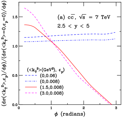
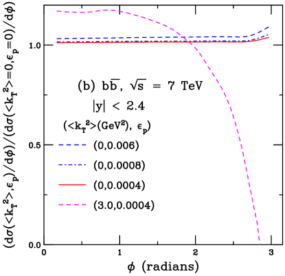
Figure 7: (Color online) The ratio of azimuthal angle distributions for the same $\langle k_{T}^{2}\rangle$ and $\epsilon_{P}$ combinations as in Fig. 6 relative to $\langle k_{T}^{2}\rangle=0$, $\epsilon_{P}=0$ for (a) $c\overline{c}$ pairs at $2.5<y<5$ and (b) $b\overline{b}$ pairs at $|y|<2.4$.

To determine the influence of the heavy quark mass and scale values on $d\sigma/d\phi$ for finite $\langle k_{T}^{2}\rangle$, the full uncertainty bands are shown in Fig. 8 for the same values of $\langle k_{T}^{2}\rangle$ and $\epsilon_{P}$ employed in Fig. 5. In this case, in addition to the central value and the upper and lower limits of the band, each mass and scale combination is also shown in the light dot-dashed curves. The results are given as histograms in both cases even though $d\sigma/d\phi$ is relatively smooth, especially for $b\overline{b}$ pairs. The differences in the shapes of the distributions are larger for charm. Thus the level of the enhancement at $\phi\sim 0$ seen for the central value varies considerably in this case.

The upper and lower limits of the band are obtained according to Eqs. (II.5) and (II.5) with $X=\phi$. On a bin-by-bin basis, the maximum and minimum mass and scale combination may vary. For example, changing the factorization scale changes the slope of the $p_{T}$ distribution so that, at some value of $p_{T}$, the maximum of $d\sigma/dp_{T}$ may come from a different scale choice. The mass and scale choices affect the shape of $d\sigma/d\phi$ most strongly for charm. As $\phi\rightarrow\pi$, the maximum of $d\sigma/d\phi$ approaches the central value while the minimum of the band is essentially determined by a single mass and scale combination.

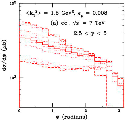
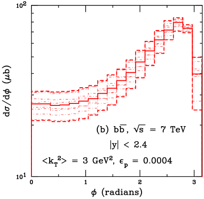
Figure 8: (Color online) The mass and scale uncertainty band on the NLO azimuthal distributions in $p+p$ collisions at $\sqrt{s}=7$ TeV using the HVQMNR code for (a) $c\overline{c}$ pairs at forward rapidity, $2.5<y<5$, and (b) $b\overline{b}$ pairs at midrapidity, $|y|<2.4$. The calculations utilize $(\langle k_{T}^{2}\rangle({\rm GeV}^{2}),\epsilon_{P})=(1.5,0.008)$ for charm and (3,0.0004) for bottom. The solid curves show the central results; the dashed, the edges of the uncertainty band; and the light dot-dashed curves are the individual mass and scale combinations.

To end this section, the effect of a $p_{T}$ cut on $d\sigma/d\phi$ for the values of $\langle k_{T}^{2}\rangle$ and $\epsilon_{P}$ used in the calculations of the uncertainty band in Figs. 5 and 8 is shown in Fig. 9. Results are given starting from low $p_{T}$, $p_{T}<10$ GeV, and increasing with $p_{T}$ cuts above 10, 20, 30, 40, 50 and 75 GeV for charm with an additional cut of $p_{T}>100$ GeV for bottom. (Note that a minimum $p_{T}$ cut is chosen instead of a $p_{T}$ range because the azimuthal distribution is dominated by the behavior at the lowest $p_{T}$.) The low $p_{T}$ results, with $p_{T}<10$ GeV, are equivalent to those integrated over all $p_{T}$, shown in Fig. 6. Notably, already at $p_{T}>10$ GeV, the shape of $d\sigma/d\phi$ changes with peaks at both $\phi=0$ and $\phi\sim\pi$ and a deepening dip developing between the two peaks. This is because that, as the minimum $p_{T}$ increases, the light parton in the $2\rightarrow 3$ process is more likely to either be low momentum and aligned with one of the two heavy quarks and opposite the other (emission from a final-state heavy quark, Fig. 2(a), $\phi\sim\pi$) or high momentum and balancing its momentum against that of the $Q\overline{Q}$ pair ($\phi\sim 0$, Fig. 2(b)-(d)).

Note that no scale factors are applied to separate the distributions, the decrease of $d\sigma/dp_{T}$ is sufficient to separate them without introducing an additional scale factor. However, in the case of charm production, while no scale factor is applied to the $p_{T}<10$ GeV distribution, the remaining distributions are multiplied by a factor of $10^{3}$ to be visible on the plot due to the steeply-falling $p_{T}$ distribution of the charm quarks.

The $c\overline{c}$ distributions are shown as histograms with per bin uncertainties because the charm quark $p_{T}$ distributions decrease with $p_{T}$ faster than those for bottom quarks so that, by $p_{T}>50$ GeV the statistics for $c\overline{c}$ pairs are poor. There are few $c\overline{c}$ events produced for $p_{T}>75$ GeV, as seen in Fig. 9(a), and these are mostly at $\phi\sim 0$. Note that the $c\overline{c}$ results are shown for the forward rapidity region, $2.5<y<5$, in the LHCb acceptance. In this rapidity range, the $p_{T}$ distributions are more steeply falling than at central rapidity because the edge of phase space for production is reached at lower $p_{T}$ at forward rapidity. However, as will be explained, the shape of $d\sigma/d\phi$ is not strongly dependent on the rapidity range.

The $b\overline{b}$ distributions in Fig. 9(b) show the same trends but the harder $p_{T}$ distributions for bottom quarks result in smoother azimuthal distributions for $b\overline{b}$ pairs even for $p_{T}>100$ GeV. The higher the $p_{T}$, the more pronounced the peak at $\phi\sim 0$ becomes while the enhancement at $\phi\sim\pi$ does not disappear. (Note that there is no enhancement at $\phi\sim 0$ for the lowest $p_{T}$ cut, $p_{T}<10$ GeV, as is the case for charm.)

While the calculations shown in Fig. 9 are for the central values of quark mass and scale factors, the trends would remain the same for all the mass and scale combinations, especially for $b\overline{b}$, see Fig. 8.

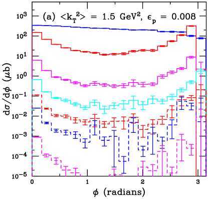
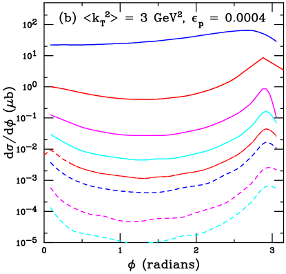
Figure 9: (Color online) The effect of changing the $p_{T}$ cut on the azimuthat angle distribution between the two heavy quarks. The calculations utilize $(\langle k_{T}^{2}\rangle({\rm GeV}^{2}),\epsilon_{P})=(1.5,0.008)$ for charm (a) and (3,0.0004) for bottom (b). The $c\overline{c}$ distributions are shown at forward rapidity, $2.5<y<5$, while the $b\overline{b}$ distributions are at midrapidity, $|y|<2.4$. From top to bottom the results are: $p_{T}<10$ GeV; $p_{T}>10$ GeV; $p_{T}>20$ GeV; $p_{T}>30$ GeV; $p_{T}>40$ GeV; $p_{T}>50$ GeV; $p_{T}>75$ GeV. The $c\overline{c}$ curves for all but the lowest $p_{T}$ cut are scaled up by $10^{3}$. The $b\overline{b}$ curves, which do not include a scale factor, also include a calculation with $p_{T}>100$ GeV.

IV Sensitivity of $d\sigma/d\phi$ to $\langle k_{T}^{2}\rangle$

In this section, the sensitivity of $d\sigma/d\phi$ to the size of the intrinsic $\langle k_{T}^{2}\rangle$ is explored to determine whether or not there is any obvious onset of the change in $d\sigma/d\phi$. Thus Eq. (3) is modified to introduce a parameter $\Delta$ that reduces the average $\langle k_{T}^{2}\rangle$,

$$\langle k_{T}^{2}\rangle=1+\frac{\Delta}{n}\ln\left(\frac{\sqrt{s}}{20\,{\rm GeV}}\right)\,\,{\rm GeV}^{2}\,\,,$$ (9)

starting with $\langle k_{T}^{2}\rangle=0$. (Note that $\Delta=1$ in Eq. (3).) For charm pair production with $n=12$, $\Delta=-3/2$, $-1$, $-1/2$, 0, 1/2, and 1, effectively changing $\langle k_{T}^{2}\rangle$ by $\sim 0.25$ GeV² at $\sqrt{s}=7$ TeV as $\Delta$ is increased by 1/2. For bottom pair production, only $\Delta=-1/2$, 0, 1/2 and 1 result in $\langle k_{T}^{2}\rangle>0$ because, with $n=3$, each change in $\Delta$ increases $\langle k_{T}^{2}\rangle$ by $\sim 1$ GeV² at $\sqrt{s}=7$ TeV. Here $\Delta=-1/2$ results in $\langle k_{T}^{2}\rangle=0.02$ GeV².

The broad $p_{T}$ cuts, $p_{T}<10$ GeV and $p_{T}>10$ GeV, are studied both at midrapidity ($|y|<2.4$) and forward rapidity ($2.5<y<5$). Only the results for midrapidity are shown here, however, since trends were found to be independent of rapidity. The figures in this section include the $c\overline{c}$ and $b\overline{b}$ azimuthal distributions, $d\sigma/d\phi$, as well as the ratios, $(d\sigma(\langle k_{T}^{2}\rangle)/d\phi)/(d\sigma(\langle k_{T}^{2}\rangle=0)/d\phi)$, to highlight the effects when differences in the distributions themselves may be small. Note that the choice of 10 GeV is somewhat arbitrary and not indicative of any threshold behavior. Comparison with data in the next section will be more indicative of the importance of $\langle k_{T}^{2}\rangle$ in a given $p_{T}$ range.

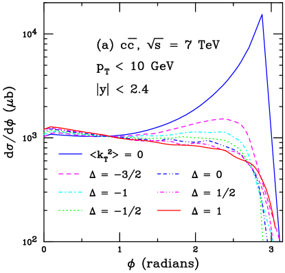
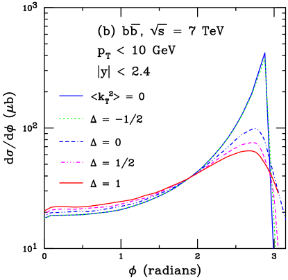
Figure 10: (Color online) The azimuthal angle distributions for (a) $c\overline{c}$ and (b) $b\overline{b}$ pairs in the central rapidity range $|y|<2.4$ with $p_{T}<10$ GeV. Calculations are shown with $\langle k_{T}^{2}\rangle=0$ and for values of $\Delta$ from $-3/2$ to 1 for charm and $\Delta=-1/2$ to 1 for bottom, as in Eq. (9).

Figure 10(a) shows the $c\overline{c}$ azimuthal distributions for $p_{T}<10$ GeV at central rapidity. Note that increasing $\langle k_{T}^{2}\rangle$ from 0 to 0.25 GeV² already shows a significant change in $d\sigma/d\phi$ for $c\overline{c}$. The peak at $\phi\sim\pi$ is largely erased and only a weak variation with $\phi$ can be seen on the log scale for $\phi<\pi/2$. As $\langle k_{T}^{2}\rangle$ increases, the enhancement at $\phi\sim 0$ increases while the peak near $\phi\sim\pi$ decreases and disappears. A similar but slower evolution is seen for $b\overline{b}$ in Fig. 10(b). Note that $\langle k_{T}^{2}\rangle=0.02$ GeV² still largely follows the $\langle k_{T}^{2}\rangle=0$ results, as may be seen in the dotted curve. Thus sufficiently small steps in $\langle k_{T}^{2}\rangle$ would likely reveal a gradual change in $d\sigma/d\phi$.

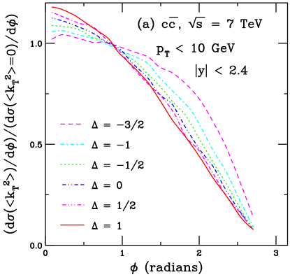
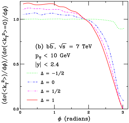
Figure 11: (Color online) The ratio of azimuthal angle distributions relative to that of $\langle k_{T}^{2}\rangle=0$ for (a) $c\overline{c}$ and (b) $b\overline{b}$ pairs in the central rapidity range $|y|<2.4$ with $p_{T}<10$ GeV. Calculations are shown for values of $\Delta$ from $-3/2$ to 1 for charm and $\Delta=-1/2$ to 1 for bottom, as in Eq. (9).

The relative changes in the distributions care seen more clearly in Fig. 11 where the ratios of the azimuthal distributions relative to that with $\langle k_{T}^{2}\rangle=0$ are shown. The charm quark ratios go from relatively flat at $\phi<\pi/2$ to an almost linear decrease with the maximum $\langle k_{T}^{2}\rangle$, with $\Delta=1$ corresponding to the red curves in Figs. 4(a) and 6(a). The ratio of the distributions pivot around $\phi\sim 1$ with a smooth evolution of the ratios with $\Delta$.

On the other hand, the $b\overline{b}$ ratios pivot around $\phi\sim 2$, from a slight modification at $\phi\sim\pi$ for $\langle k_{T}^{2}\rangle=0.02$ GeV² to a flat ratio for $\phi<2$ followed by a steep descent for $\phi>2$.

The difference in the location of the pivot point of the distributions is due to the heavy quark mass. The lighter mass of the charm quarks makes it more likely that their relative momentum will become more isotropic at low $p_{T}$ as $\Delta$ increases. Thus the point around which the slope of the ratio is changing is closer to $\phi\sim 0$. The bottom quarks, more than three times more massive than the charm quarks, are less likely to have their azimuthal distributions become completely isotropic at low $p_{T}$ since the $k_{T}$ kicks are less effective on heavier quarks. Thus there is a reduced peak at $\phi\sim\pi$ for $b\overline{b}$ and the slopes of the ratios pivot at an angle closer to $\phi\sim\pi$.

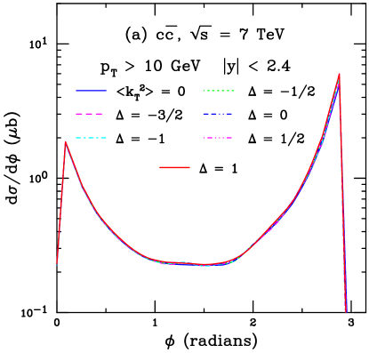
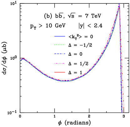
Figure 12: (Color online) The azimuthal angle distributions for (a) $c\overline{c}$ and (b) $b\overline{b}$ pairs in the central rapidity range $|y|<2.4$ with $p_{T}>10$ GeV. Calculations are shown with $\langle k_{T}^{2}\rangle=0$ and for values of $\Delta$ from $-3/2$ to 1 for charm and $\Delta=-1/2$ to 1 for bottom, as in Eq. (9).

Figures 12 and 13 show $d\sigma/d\phi$ for $p_{T}>10$ GeV at midrapidity and the ratios relative to $d\sigma/d\phi$ with $\langle k_{T}^{2}\rangle=0$. In this case, an enhancement is seen at $\phi\sim 0$ for both charm and bottom although the enhacement is larger for charm (note that the scales on the $y$-axes of Fig. 13 are the same). The shapes are consistent with the solid red distributions in Fig. 9.

It is not possible to distinguish between different values of $\Delta$ for $c\overline{c}$, even by examining the ratios in Fig. 13(a). Although the ratios increase with $\Delta$ at $\phi\sim 0$, the curves are almost indistinguishable at low $\phi$. Larger differences in the $c\overline{c}$ ratios as $\phi\rightarrow\pi$ can be observed since the ratios at $\phi>2.5$ increase at slightly lower $\phi$ for higher values of $\langle k_{T}^{2}\rangle$. This is because $\langle k_{T}^{2}\rangle^{1/2}<p_{T}$ for all $p_{T}$, resulting in a negligible effect for charm. There is also only a small difference between the $b\overline{b}$ ratios in Fig. 13(b). However, the $b\overline{b}$ ratios are visibly separated at $\phi\sim 0$ because $\langle k_{T}^{2}\rangle^{1/2}<p_{T}$ remains true for the heavier bottom quarks, $\langle k_{T}^{2}\rangle^{1/2}/p_{T}\sim 0.1-0.2$ for bottom, rather than $\langle k_{T}^{2}\rangle^{1/2}/p_{T}\sim 0.05-0.1$ for charm. In addition, the harder $p_{T}$ distribution for bottom means that a smaller fraction of the total $b\overline{b}$ cross section is contained the region $p_{T}<10$ GeV than for charm where $\sim 98$% of the charm $p_{T}$ distribution is contained in the range $p_{T}<10$ GeV.

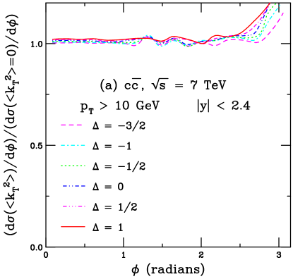
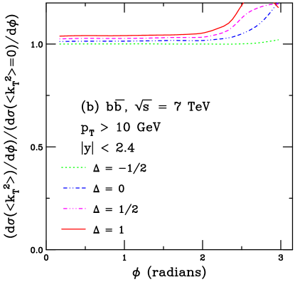
Figure 13: (Color online) The ratio of azimuthal angle distributions relative to that of $\langle k_{T}^{2}\rangle=0$ for (a) $c\overline{c}$ and (b) $b\overline{b}$ pairs in the central rapidity range $|y|<2.4$ with $p_{T}>10$ GeV. Calculations are shown for values of $\Delta$ from $-3/2$ to 1 for charm and $\Delta=-1/2$ to 1 for bottom, as in Eq. (9).

Finally, it is worth noting that the azimuthal angle distributions and their ratios at low $p_{T}$ ($p_{T}<10$ GeV) and higher $p_{T}$ ($p_{T}>10$ GeV) at forward rapidity are effectively identical to those at midrapidity. Thus, these results are not shown. Results for $p_{T}$ cuts higher than $p_{T}>10$ GeV are not shown because the effect of $k_{T}$ broadening on higher $p_{T}$ cuts would be negligible.

V Comparison to Data

There are data on heavy quark pair correlations to test these calculations. There are charm pair correlation data from ALICE ALICEDDpairs and LHCb LHCbDDpairs and bottom quark-bottom jet correlations from CMS CMSbbpairs , both from $p+p$ collisions at $\sqrt{s}=7$ TeV. In addition, there are $D^{0}D^{*-}$ and $D^{+}D^{*-}$ data from $p+\overline{p}$ collisions at $\sqrt{s}=1.96$ TeV from CDF in Tevatron Run II CDFDDpairs .

V.1 LHCb $C\overline{C}$ Data

LHCb measured $c\overline{c}$, $cc$, and $(c+\overline{c})J/\psi$ correlations in $p+p$ collisions at 7 TeV for $2<y<4$ and $3<p_{T}<12$ GeV. The discussion here will focus on comparison to some of the $c\overline{c}$ correlations, in particular on the $D^{0}\overline{D}^{0}$, $D^{0}D^{-}$ and $D^{+}D^{-}$ combinations where fragmentation functions are known. Thus final states that include a $D_{s}$ or $\Lambda_{c}$ are excluded. In addition, the final-state $c\overline{c}$ data measured by LHCb are more likely to arise from production of a single $c\overline{c}$ pair.

Figure 14 shows the azimuthal angle distributions for the same values of $\Delta$ (from Eq. (9)) employed in the previous section. The results for $\phi<2$ are in good agreement with the data and with the results of Fig. 12(a) for $p_{T}>10$ GeV. However, as $\phi\rightarrow\pi$, there is a strong effect on the peak value as a function of $\Delta$. The peak in this region gets broader and lower as $\Delta$ increases. The larger values of $\Delta$ are closer to the data although the data show only a slight trend upward in this region rather than a second peak at $\phi\sim\pi$. The calculations at large $\phi$ differ strongly with those at $p_{T}>10$ GeV in Fig. 12(a), likely because at $p_{T}\sim 3$ GeV a significant contribution from $k_{T}$ broadening still remains, see Fig. 4. The sharp peak near $\phi\sim\pi$ is somewhat artificial since, at $\langle k_{T}^{2}\rangle=0$, all the peak is essentially contained in a single $\Delta\phi$ bin. When $k_{T}$ broadening is included, the peak region is wider and is shared among several bins although, for $p_{T}$ values of a few GeV, not including $p_{T}<2\langle p_{T}\rangle\sim 2m_{D}$, it is not completely washed out as it is for the results with $p_{T}<10$ GeV, dominated by $p_{T}\sim 0$, in Fig. 10. Thus the overall agreement of the calculations with the LHCb $\phi$ distribution data can be considered quite good.

Figure 14: (Color online) The azimuthal angle distributions for $D^{0}\overline{D}^{0}$ (red), $D^{0}D^{-}$ (blue), and $D^{+}D^{-}$ (magenta) pairs measured in $p+p$ collisions at $\sqrt{s}=7$ TeV by LHCb LHCbDDpairs . The data are compared to calculations in the same acceptance with $\langle k_{T}^{2}\rangle=0$ and for values of $\Delta$ from $-3/2$ to 1 in Eq. (9).

Calculations of the $D\overline{D}$ pair invariant mass in the LHCb acceptance with the data are shown in Fig. 15. The agreement of the calculations with the data are very good. A similar minimum is seen in both for $M\sim 2\sqrt{m_{D}^{2}+p_{T}^{2}}\sim 7$ GeV, using the lower limit of the $p_{T}$ range for the detected $D$ mesons. Below this value of $M$, the data have a higher cross section than the calculations. The gap in the calculated mass at $M\sim 7$ GeV for $\langle k_{T}^{2}\rangle=0$ fills in as $\Delta$ increases. In addition, at higher masses, the calculated distribution falls off somewhat faster for larger $\Delta$ so that $\Delta=1$ agrees best with the data.

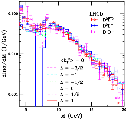
Figure 15: (Color online) The invariant mass distributions for $D^{0}\overline{D}^{0}$ (red), $D^{0}D^{-}$ (blue), and $D^{+}D^{-}$ (magenta) pairs measured in $p+p$ collisions at $\sqrt{s}=7$ TeV by LHCb LHCbDDpairs . The data are compared to calculations in the same acceptance with $\langle k_{T}^{2}\rangle=0$ and for values of $\Delta$ from $-3/2$ to 1 in Eq. (9).

Finally, Fig. 16 compares the data with the calcualated $|\Delta y|$ distribution. In this case, the calculated results are independent of the $k_{T}$ broadening. The data fall off somewhat faster than the calculations in all cases.

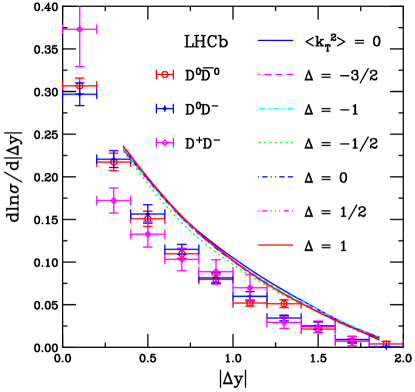
Figure 16: (Color online) The $|\Delta y|$ distributions for $D^{0}\overline{D}^{0}$ (red), $D^{0}D^{-}$ (blue), and $D^{+}D^{-}$ (magenta) pairs measured in $p+p$ collisions at $\sqrt{s}=7$ TeV by LHCb LHCbDDpairs . The data are compared to calculations in the same acceptance with $\langle k_{T}^{2}\rangle=0$ and for values of $\Delta$ from $-3/2$ to 1 in Eq. (9).

Overall, the calculated results are in good agreement with the assumption that the $D$ and $\overline{D}$ mesons both arise from the production of a single $c\overline{c}$ pair. Discrepancies between the calculations and the data may appear because the calculations are based on exclusive $Q\overline{Q}$ production and include only real corrections at next-to-leading order in addition to vertex corrections. No soft radiation from parton showers, as in event generators, which might smooth out the $\Delta\phi$ distribution at $\phi\sim\pi$, are included in these calculations, only fragmentation. In addition, HVQMNR is a negative weight Monte Carlo so that additional weight is placed on the last $\phi$ bin, $\phi=\pi$. A positive weight next-to-leading order exclusive Monte Carlo, such as POWHEG, can be coupled to PYTHIA or HERWIG and include soft initial or final-state radiation. If the multiplicities of the $p+p$ events are sufficiently large, heavy quark scattering with produced particles may also weaken the azimuthal correlation. See Ref. Szczurek for a comparison of these data to calculations in the $k_{T}$-factorization approach.

Note also that, while most of the events are likely to arise from production of a single $c\overline{c}$ pair, the $cc$ and $(c+\overline{c})J/\psi$ yields constitute about 10% of the total charm hadron pair yields LHCbDDpairs . Because only the $c\overline{c}$ pairs can be produced in a single hard scattering, these other events are more consistent with production through double parton scattering or independent production of two $c\overline{c}$ pairs. The azimuthal and rapidity distributions for the $cc$ and $cJ/\psi$ events are consistent with isotropic production LHCbDDpairs , as might be expected from two hard scatterings.

In addition the ALICE Collaboration made an analysis of azimuthal correlations between reconstructed $D$ mesons and a light hadron trigger particle in $p+p$ collisions at 7 TeV and $p+$Pb collisions at 5.02 TeV ALICEDDpairs . The light hadrons were primary particles, emitted from the collision points. These particles include those from heavy flavor decays, such as the unreconstructed partner $D$ meson. The data were binned according to the transverse momentum of both the $D$ meson and the light hadron. The minimum light hadron $p_{T}$ was soft, $p_{T}>0.3$ GeV. These data were further subdivided into two $p_{T}$ ranges, $0.3<p_{T}<1$ GeV and $p_{T}>1$ GeV. The $D$ meson $p_{T}$ was considerably higher: $3<p_{T}<5$ GeV, $5<p_{T}<8$ GeV, and $8<p_{T}<16$ GeV. To improve statistics, the “$D$ meson” is an average over the $D^{0}$, $D^{+}$ and $D^{*+}$. The ALICE measurements cover the central region, $|y|<0.5$ for the $D$ and $|\Delta\eta|<1$ for the light hadron. The general behavior is, however, the same as the LHCb $D^{0}\overline{D}^{0}$ pairs, a peak at $\Delta\phi=0$ and a smaller enhancement at $\Delta\phi=\pi$. The peak at $\Delta\phi=0$ increases with increasing trigger particle $p_{T}$ and also with increasing $D$ meson $p_{T}$ consistent with the trends of these calculations. The data were compared to simulations with various PYTHIA tunes and also POWHEG+PYTHIA. All simulations reproduced the trends of the data ALICEDDpairs , consistent with what one might expect from the results shown here. New ALICE data on $D$-hadron correlations in $p+p$ collisions at 13 TeV were presented recently BTrzeciak . In these higher energy collisions, the same models describe these data as well.

V.2 CDF $D\overline{D}$ Data

The CDF Collaboration studied charm hadron correlations in $p+\overline{p}$ collisions at $\sqrt{s}=1.96$ TeV CDFDDpairs . CDF combined their single inclusive charm hadron data to look for fully reconstructed charm quark pairs. Only $D^{*\pm}$ were considered as candidates for the second charm hadron, in the decay chain $D^{*\pm}\rightarrow(D^{0}/\overline{D}^{0})\pi^{\pm}\rightarrow(K\pi)\pi^{\pm}$, so that the mass difference between the $D^{*\pm}$ and the first charm hadron, $D^{0}/\overline{D}^{0}$ or $D^{\pm}$, $\Delta m=m(K\pi\pi)-m(K\pi)$, can suppress the combinatorial background. Several thousand $D^{0}D^{*-}$ and $D^{+}D^{*-}$ pairs were constructed in this way.

Their goal was to try to better understand the underlying $Q\overline{Q}$ production process CDFDDpairs . As discussed in Sec. II.3, commonly employed high energy event generators such as PYTHIA implement prompt $Q\overline{Q}$ production by three different leading-order porcesses: ‘pair creation’, as in the LO diagrams in Fig. 1; ‘flavor excitation’, and ‘gluon splitting’, corresponding to the NLO processes shown in Fig. 2 (b) and (c) respectively.

The weighting of these different contributions in PYTHIA can be tuned to match the data to determine which processes are most important to heavy flavor production in the phase space covered by an experiment. According to this interpretation, the final-state $Q\overline{Q}$ configurations are treated separately by virtue of their topology with $\phi=\pi$, corresponding to pair creation, and $\phi=0$, corresponding to gluon splitting. This apporach stands in contrast to the NLO calculations shown in this paper where all NLO diagrams are summed coherently with weighting according to color and spin with interference terms. As described in Sec. II.3, at NLO, flavor excitation and gluon splitting are both part of production by $gg$ interactions in the initial state. They are not separate production processes and are not treated as such.

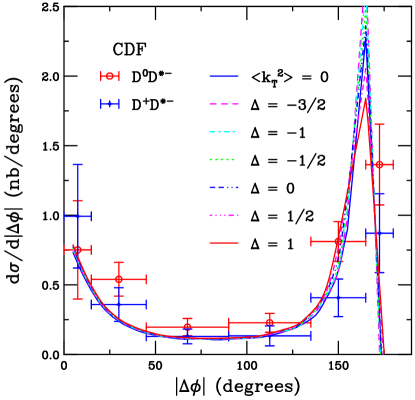
Figure 17: (Color online) The azimuthal angle distributions for $D^{0}D^{*-}$ (red) and $D^{+}D^{*-}$ (blue) pairs measured in $p+\overline{p}$ collisions at $\sqrt{s}=1.96$ TeV by CDF CDFDDpairs . The data are compared to calculations in the same acceptance with $\langle k_{T}^{2}\rangle=0$ and for values of $\Delta$ from $-3/2$ to 1 in Eq. (9).

The data on each final state, in the rapidity interval $|y|<1$ and $p_{T}$ ranges $5.5<p_{T}^{D^{0},D^{*-}}<20$ GeV, $7<p_{T}^{D^{+}}<20$ GeV, are shown in Fig. 17. In the calculations, the $y$ interval was the same but the lower limit on the $D$ meson $p_{T}$ was taken to be 5.5 GeV in all cases. The calculations agree rather well with the data. The results are independent of $\Delta$ except when the pairs are completely back-to-back ($|\Delta\phi|=\pi$), as might be expected for the given $p_{T}$ range. In Ref. CDFDDpairs , the comparison with the separate LO ‘production mechanisms’ in PYTHIA showed that, at least for the PYTHIA tune used by the CDF Collaboration, the ’gluon splitting’ or collinear contribution ($\Delta\phi=0$) to production was underestimated. In the calculation, with the NLO contributions added according to initial-state parton channel ($gg$, $(q/\overline{q})g$ and $q\overline{q}$), there is no significant discrepancy.

V.3 CMS Bottom Quark-Bottom Jet Data

The CMS Collaboration measured $b\overline{b}$ correlations through the use of their jet trigger CMSbbpairs . The analysis employed the single jet trigger with calorimeter energy above trigger thresholds of 15, 30 and 45 GeV. The energy scale at which these three triggers are greater than 99% efficient corresponds to transverse momentum of the leading jet, $p_{T}^{\rm jet}$, of 56, 84 and 120 GeV respectively. The leading jet is associated with one of the $b$ quarks. The triggered events are required to have one reconstructed jet with the minimum $p_{T}$ defined as above and a reconstructed primary vertex. The leading jet is requred to be within the pseudorapidity interval $|\eta^{\rm jet}|<3$. The jet along with identified $B$ hadrons with $p_{T}^{B}>15$ GeV and in the interval $|\eta^{B}|<2$, is considered to originate from a single $b\overline{b}$ pair. Thus the events also have two reconstructed secondary vertices. The angular correlations are calculated using the $B$ hadron and $b$-jet flight directions.

The CMS results were presented as a function of the azimuthal angle difference, $\Delta\phi$, and a separation variable, $\Delta R$, that includes the difference in polar angles between the $B$ hadron and jet, given in terms of the difference in pseudorapidity, $\Delta\eta$, $\Delta R=\sqrt{(\Delta\eta)^{2}+(\Delta\phi)^{2}}$. The CMS predictions for the behavior of $\Delta R$ are based on the notion that gluon splitting dominates at low $\Delta R$ while flavor creation is most important at large $\Delta R$. This is similar to what one expects from event generators for $\Delta\phi$, as discussed in Secs. II.3 and V.2.

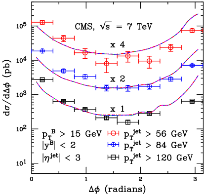
Figure 18: (Color online) The azimuthal angle distributions for $B\overline{B}$ pairs measured in $p+p$ collisions at $\sqrt{s}=7$ TeV by CMS CMSbbpairs . The $p_{T}^{\rm jet}$ lower limits of 56 GeV (red), 84 GeV (blue) and 120 GeV (black) are scaled by factors of 4, 2 and 1 respectively. The data are compared to calculations in the same kinematics for $\langle k_{T}^{2}\rangle=0$ (blue curves) and for values of $\Delta$ from $-1/2$ to 1 in Eq. (9).

The calculations shown here are based on the assumption that a $b\overline{b}$ pair is produced with one final state $B$ or $\overline{B}$ in the kinematic region $p_{T}^{B}>15$ GeV and rapidity $|y^{B}|<2$. The jet is assumed to originate from the second $B$ hadron of the pair with the minimum $p_{T}$ of the $B$ equal to the $p_{T}$ of the jet, greater than 56, 84 and 120 GeV respectively, while $\eta^{\rm jet}$ is assumed to be equivalent to the rapidity of the $b$ quark. Since the pseudorapidity difference is replaced by a rapidity difference in the calculation of $\Delta R$ and the equivalence of the $b$ quark and the jet $p_{T}$ might not be exact, one might expect that the calculation of the $\Delta\phi$ distribution might be better reproduced than that of $\Delta R$.

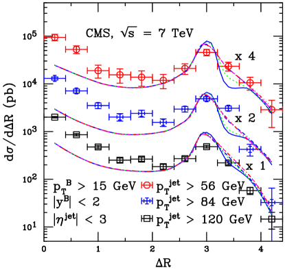
Figure 19: (Color online) The $\Delta R$ distributions for $B\overline{B}$ pairs measured in $p+p$ collisions at $\sqrt{s}=7$ TeV by CMS CMSbbpairs . The $p_{T}^{\rm jet}$ lower limits of 56 GeV (red), 84 GeV (blue) and 120 GeV (black) are scaled by factors of 4, 2 and 1 respectively. The data are compared to calculations in the same kinematics for $\langle k_{T}^{2}\rangle=0$ (blue curves) and for values of $\Delta$ from $-1/2$ to 1 in Eq. (9), the green dotted to solid red curves respectively.

The comparisons of the calculations with the data are shown in Figs. 18 and 19. While the calculations are done with all values of $\Delta$ in Eq. (9), no difference between them is visible except at large $\Delta R$. As in Ref. CMSbbpairs , the data and calculations for the different minimum jet $p_{T}$ are scaled by factors of 4, 2 and 1 for $p_{T}^{\rm jet}$ greater than 56, 84 and 120 GeV respectively to more clearly separate the results.

The comparison to the $\Delta\phi$ distributions is very good, as may be expected. The comparison to $\Delta R$ is not as good at low $\Delta R$ where the CMS Collaboration suggests gluon splitting is dominant. However, given the agreement with the low $\Delta\phi$ results, where this mechanism is also expected to be dominant in event generators, the underestimate may be due to the calculation of $\Delta R$ with $\Delta y$ instead of $\Delta\eta$. Note that the large $\Delta R$ results are best reproduced with $\Delta=1$ in Eq. (9).

VI Cold Nuclear Matter: $p+$Pb Collisions at 5.02 TeV

Finally, the interaction of $c\overline{c}$ pairs in cold nuclear matter, such as $p+$Pb collisions at the LHC, are discussed. It has been suggested gossiaux that energy loss by heavy quarks in heavy-ion collisions could change the azimuthal correlations. First, it must be determined how the charm distributions and their azimuthal separation are influenced by the presence of cold nuclear matter. For example, the effect of cold matter energy loss, which could be manifested as additional $k_{T}$ broadening by multiple scattering in the nucleus, could result in changes in the $p_{T}$ distributions of heavy quarks in $p+$Pb relative $p+p$ collisions. This would be in addition to modification of the parton densities in the nucleus, referred to as shadowing.

Here the results of shadowing alone on the single charm meson $p_{T}$ distributions and $c\overline{c}$ pair azimuthal distributions are compared to shadowing and $k_{T}$ broadening, both with $\langle k_{T}^{2}\rangle\sim 1.5$ GeV² alone, as in $p+p$ collisions, and with an additional $k_{T}$ kick due to the presence of the nuclear medium in $p+$Pb collisions.

The calculations of the nuclear modification factor $R_{p{\rm Pb}}(p_{T})$ are compared to data from ALICE ALICEDmesons . ALICE measured prompt production of $D^{0}$, $D^{+}$, $D^{*+}$, and $D_{s}^{-}$ as well as their charge conjugates at central rapidity, $-0.96<y_{\rm cms}<0.04$ in $p+$Pb collisions at $\sqrt{s}=5.02$ TeV. The yields were compared to those in $p+p$ collisions to form $R_{p{\rm Pb}}(p_{T})$. Note that, for the analysis in Ref. ALICEDmesons , the $p+p$ baseline at 5.02 TeV was interpolated between the 2.76 TeV and 7 TeV data since it was completed before $p+p$ data were available at 5.02 TeV.

In Ref. ALICEDmesons , the average of the $D^{0}$, $D^{+}$ and $D^{*+}$ were compared to several calculations, including next-to-leading order calculations with HVQMNR including only shadowing effects with no momentum braodening nor fragmentation. The uncertainty band gives suppression below $p_{T}\sim 5$ GeV, rising to be equivalent with unity at higher $p_{T}$. See Ref. ALICEDmesons for details of the other comparisons which included a leading order calculation of shadowing due to power corrections, $k_{T}$ broadening and cold matter energy loss Vitev , and a calculation assuming color glass condensate in the initial state Fuji .

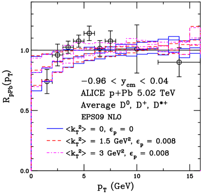
Figure 20: (Color online) The nuclear modification factor $R_{p{\rm Pb}}(p_{T})$ in 5.02 TeV $p+$Pb collisions for $-0.96<y_{\rm cm}<0.04$. The ALICE data for the average of their $D^{0}$, $D^{+}$ and $D^{*+}$ measurements ALICEDmesons at central rapidity are shown. Results are shown for: no $k_{T}$ broadening and no fragmentation (solid blue); the standard result from Sec. III, $\langle k_{T}^{2}\rangle=1.5$ GeV² and $\epsilon_{P}=0.008$ (red dashed); and $\langle k_{T}^{2}\rangle=3$ GeV² and $\epsilon_{P}=0.008$ (magenta dot-dashed). The EPS09 NLO uncertainty band, along with the central value, is shown. Note that the additional $k_{T}$ broadening is only applied to $p+$Pb collisions and not to $p+p$ collisions in the magenta curves.

To go beyond $p+p$ collisions, in the NLO calculations, the proton parton densities must be replaced by those of the nucleus. If $A$ is a nucleus, the nuclear parton densities, $f_{i}^{A}(x_{2},\mu^{2})$, can be assumed to factorize into the nucleon parton density, $f_{i}^{p}(x_{2},\mu_{F}^{2})$, independent of $A$; and a shadowing ratio, $S_{i}(A,x_{2},\mu_{F}^{2})$ that parameterizes the modifications of the nucleon parton densities in the nucleus. Here $x_{2}$ is the fraction of the nucleon momentum carried by the interacting parton in the nucleus. While the shadowing effect may also depend on the impact parameter, $b$, of the parton from the proton with the lead nucleus, only minimum bias results, independent of impact parameter, are shown here.

The calculations in Fig. 20 employ the EPS09 NLO EPS09 parameterization for $S_{i}$, assuming collinear factorization. The EPS09 sets include 15 parameters, giving an error set of 30 additional parameterizations created by varying each parameter within one standard deviation. The EPS09 uncertainty band is obtained by calculating the deviations from the central value for the 15 parameter variations on either side of the central set and adding them in quadrature. There is a more recent shadowing parameterization by Eskola et al., EPPS16 EPPS16 , that includes some of the LHC data from the first $p+$Pb run at 5.02 TeV in the global analysis of the nuclear parton densities. The central result for the gluon distribution is very similar to that of EPS09 so that the central result with EPPS16 should be very similar to that shown here. However, it employs 5 additional parameters, thus resulting in a larger uncertainty band than the one in Fig. 20.

The calculations given as a function of $p_{T}$ in Fig. 20 are in the same rapidity interval as the ALICE data. Three bands are shown. The first, with $\langle k_{T}^{2}\rangle=0$ and $\epsilon_{P}=0$, in blue, corresponds to the EPS09 calculation in Ref. ALICEDmesons albeit the curves in that paper likely employed a larger quark mass, $m\sim 1.5$ GeV, which would result in a reduced shadowing effect at $p_{T}\sim 0$ relative to the calculation shown here. The red histogram, employing the preferred parameters found for $D$ mesons in this paper, and assuming the same intrinsic $k_{T}$ in $p+$Pb and $p+p$ collisions, gives a nearly identical result to the blue histogram, calculated without either effect.

However, one might expect that a higher intrinsic $k_{T}$ is required in a nuclear medium relative to that in $p+p$ due to multiple scattering in the nucleus, known as the Cronin effect Cronin . If one assumes that $\langle k_{T}^{2}\rangle$ is doubled in the cold nuclear medium, then the magenta curves are obtained. The larger $\langle k_{T}^{2}\rangle$ results in an increase of the band at intermediate $p_{T}$, with the upper limit of the band increasing above unity at $p_{T}\sim 5$ GeV. The statistics on the averaged $D$ meson data are not sufficiently significant to distinguish between the results: all are consistent with the data.

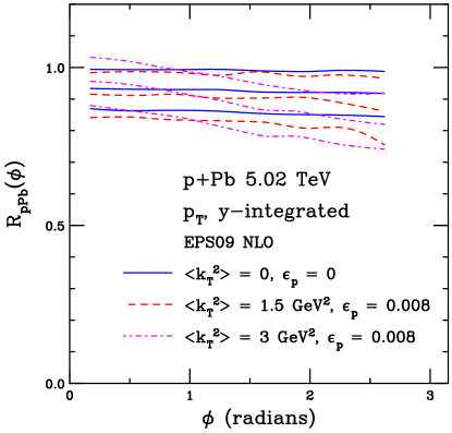
Figure 21: (Color online) The nuclear modification factor $R_{p{\rm Pb}}(\phi)$ in 5.02 TeV $p+$Pb collisions. Results are shown for: no $k_{T}$ broadening and no fragmentation (solid blue); the standard result from Sec. III, $\langle k_{T}^{2}\rangle=1.5$ GeV² and $\epsilon_{P}=0.008$ (red dashed); and $\langle k_{T}^{2}\rangle=3$ GeV² and $\epsilon_{P}=0.008$ (magenta dot-dashed). The EPS09 NLO uncertainty band is shown along with the central value. No $p_{T}$ or rapidity cuts have been imposed. Note that the additional $k_{T}$ broadening in the magenta curves is only applied to $p+$Pb collisions and not to $p+p$ collisions.

The results for the nuclear modification factor of the azimuthal angular correlations between the heavy quarks are shown in Fig. 21 for the same three sets of calculations as in Fig. 20. In this case there are no cuts made on $p_{T}$ or rapidity.

When no intrinsic $k_{T}$ is included, $R_{p{\rm Pb}}(\phi)$ is independent of $\phi$. There is a slight $\phi$ dependence introduced when the $p+p$ value of $\langle k_{T}^{2}\rangle$ is employed. It is, however, a small deviation relative to the calculation with no $k_{T}$ effect. There is a more significant effect, as expected, when the intrinsic $k_{T}$ effect is doubled in $p+$Pb relative to $p+p$ collisions. Instead of being independent of $\phi$, $R_{p{\rm Pb}}(\phi)$ now decreases as $\phi$ increases, a result of the increased $\langle k_{T}^{2}\rangle$, as in Fig. 7(a).

In heavy-ion collisions, in particular at heavy-ion colliders, multiple $c\overline{c}$ pairs are produced in a single event. Therefore, for an analysis of heavy-flavor azimuthal correlations in hot matter it is necessary to find the pair vertex to ensure that the $c$ and $\overline{c}$ originate from the same hard scattering.

VII Summary

The similarity of the results for $p_{T}>10$ GeV, even for $\langle k_{T}^{2}\rangle=0$, shows that the enhancement at $\phi\sim 0$, with the $Q\overline{Q}$ pair aligned opposite a hard parton, is independent of $\langle k_{T}^{2}\rangle$ and arises instead from the $Q\overline{Q}$ production mechanism at high $p_{T}$. Thus the high $p_{T}$ behavior of $d\sigma/d\phi$ is indicative of the contribution of next-to-leading order production while the low $p_{T}$ behavior of $d\sigma/d\phi$ is extremely sensitive to the chosen $\langle k_{T}^{2}\rangle$ and essentially independent of fragmentation.

It appears that, so far, the open heavy flavor results presented by the LHC collaborations, both single inclusive production and charm pair correlations, are in agreement with calculations based on collinear factorization with single hard scatterings. The exception, the $cc$ and $cJ/\psi$ events at LHCb, are consistent with double parton scattering.

Thus, for $p_{T}$ cuts on the order of a few GeV, the calculations of the azimuthal angle distributions are rather insensitive to fragmentation and $k_{T}$ broadening which affect the correlations at low $p_{T}$. Thus, hot nuclear matter effects on these correlations should be rather robust for $p_{T}\geq 3-5$ GeV.

References

- (1) A. Mischke, A new correlation method to identify and separate charm and bottom production processes at RHIC, Phys. Lett. B 671, 361 (2009).
- (2) G. Aarts et al., Heavy-flavor production and medium properties in high-energy nuclear collisions - What next?, Eur. Phys. J. A 53, 93 (2017).
- (3) M. Nahrgang, J. Aichelin, P. B. Gossiaux and K. Werner, Azimuthal correlations of heavy quarks in Pb + Pb collisions at TeV at the CERN Large Hadron Collider, Phys. Rev. C 90, 024907 (2014).
- (4) C. Mironov, R. Vogt and G. J. Kunde, Dilepton-tagged Q anti-Q jet events at the LHC, Eur. Phys. J. C 61, 893 (2009).
- (5) L. Vermunt et al., Influence of final-state radiation on heavy-flavour observables in collisions, arXiv:1710.09639 [nucl-th].
- (6) R. Maciula and A. Szczurek, Open charm production at the LHC - -factorization approach, Phys. Rev. D 87, 094022 (2013).
- (7) M. Cacciari, M. Greco and P. Nason, The spectrum in heavy flavor hadroproduction, JHEP 05, 007 (1998).
- (8) B. A. Kniehl, G. Kramer, I. Schienbein and H. Spiesberger, Inclusive production in collisions with massive charm quarks, Phys. Rev. D 71, 014018 (2005).
- (9) M. L. Mangano, P. Nason, and G. Ridolfi, Heavy quark correlations in hadron collisions at next-to-leading order, Nucl. Phys. B 373, 295 (1992).
- (10) R. Vogt, Determining the Uncertainty on the Total Heavy Flavor Cross Section Eur. Phys. J. C 61, 793 (2009).
- (11) R. E. Nelson, R. Vogt and A. D. Frawley, Narrowing the uncertainty on the total charm cross section and its effect on the cross section, Phys. Rev. C 87, 014908 (2013).
- (12) P. Nason, S. Dawson and R. K. Ellis, The Total Cross Section for the Production of Heavy Quarks in Hadronic Collisions, Nucl. Phys. B 303 (1988) 607.
- (13) P. Nason, S. Dawson and R. K. Ellis, The One Particle Inclusive Differential Cross Section for Heavy Quark Production in Hadronic Collisions, Nucl. Phys. B 327, 49 (1988); B 335, 260(E) (1990).
- (14) W. Beenakker, H. Kuijf, W. L. van Neerven and J. Smith, QCD Corrections to Heavy Quark Production in Collisions, Phys. Rev. D 40, 54 (1989).
- (15) W. Beenakker et al., QCD corrections to heavy quark production in hadron-hadron collisions, Nucl. Phys. B 351, 507 (1991).
- (16) M. Cacciari and M. Greco, Large hadroproduction of heavy quarks, Nucl. Phys. B 421, 530 (1994).
- (17) J. Binnewies, B. A. Kniehl and G. Kramer, Predictions for photoproduction at HERA with new fragmentation functions from LEP-1, Phys. Rev. D 58, 014014 (1998).
- (18) J. Adam et al. [ALICE Collaboration], -meson production in -Pb collisions at 5.02 TeV and in pp collisions at 7 TeV, Phys. Rev. C 94, 054908 (2016).
- (19) R. Aaij et al. (LHCb Collaboration), Prompt charm production in pp collisions at TeV, Nucl. Phys. B 871, 1 (2013).
- (20) R. Aaij et al. [LHCb Collaboration], Measurements of prompt charm production cross-sections in collisions at TeV, JHEP 1603, 159 (2016), Erratum: [JHEP 1609, 013 (2016)], Erratum: [JHEP 1705, 074 (2017)]
- (21) S. Frixione, P. Nason, and G. Ridolfi, A positive-weight next-to-leading-order Monte Carlo for heavy flavour hadroproduction, JHEP 0709, 126 (2007); arXiv:0707.3081 [hep-ph].
- (22) T. Sjostrand et al., High-energy physics event generation with PYTHIA 6.1, Comput. Phys. Commun. 135, 238 (2001); arXiv:hep-ph/0308153.
- (23) G. Corcella et al., HERWIG 6: An event generator for hadron emission reactions with interfering gluons (including supersymmetric processes), JHEP 0101, 010 (2001).
- (24) M. Bedjidian et al., Hard probes in heavy ion collisions at the LHC: Heavy flavor physics, arXiv:hep-ph/0311048.
- (25) M. L. Mangano, P. Nason, and G. Ridolfi, Fixed target hadroproduction of heavy quarks, Nucl. Phys. B 405, 507 (1993).
- (26) Y. Q. Ma and R. Vogt, Quarkonium Production in an Improved Color Evaporation Model, Phys. Rev. D 94, 114029 (2016).
- (27) R. E. Nelson, R. Vogt and A. D. Frawley, in preparation.
- (28) C. Peterson, D. Schlatter, I. Schmitt, and P. Zerwas, Scaling Violations in Inclusive Annihilation Spectra, Phys. Rev. D 27 (1983) 105.
- (29) M. Cacciari, P. Nason and R. Vogt, QCD predictions for charm and bottom production at RHIC, Phys. Rev. Lett. 95, 122001 (2005).
- (30) M. Cacciari and P. Nason, Charm cross sections for the Tevatron Run II, JHEP 0309, 006 (2003).
- (31) H. L. Lai, M. Guzzi, J. Huston, Z. Li, P. Nadolsky, J. Pumplin, C.-P. Yuan, New parton distributions for collider physics, Phys. Rev. D 82, 074024 (2010).
- (32) G. Aad et al. [ATLAS Collaboration], Measurement of the -hadron production cross section using decays to final states in pp collisions at TeV with the ATLAS detector, Nucl. Phys. B 864, 341 (2012).
- (33) J. Chrin, Heavy Quark Fragmentation Functions in Annihilation, Annals N. Y. Acad. Sci. 535, 131 (1988).
- (34) R. Vogt, Phenomenology of charm and bottom production, Z. Phys. C 71, 475 (1996).
- (35) R. Vogt, The usage of the factor in heavy ion physics, Acta Phys. Hung. A 17, 75 (2003).
- (36) J. Adam et al. [ALICE Collaboration], Measurement of azimuthal correlations of D mesons and charged particles in pp collisions at TeV and p-Pb collisions at TeV, Eur. Phys. J. C 77, 245 (2017).
- (37) R. Aaij et al. [LHCb Collaboration], Observation of double charm production involving open charm in pp collisions at = 7 TeV, JHEP 1206, 141 (2012), [JHEP 1403, 108 (2014)].
- (38) V. Khachatryan et al. [CMS Collaboration], Measurement of Angular Correlations based on Seconary Verte Reconstruction at TeV, JHEP 1105, 136 (2011).
- (39) B. Reisert et al. [CDF Collaboration], Charm Production Studies at CDF, Nucl. Phys. Porc. Suppl. 170, 243 (2007).
- (40) B. Trzeciak [ALICE Collaboration], Measurements of heavy-flavor correlations and jets with ALICE at the LHC, Quark Matter 2018, https://indico.cern.ch/event/656452/contributions/2869932/
- (41) B. Abelev et al. [ALICE Collaboration], Measurement of Prompt -Meson Production in Pb Collisions at TeV, Phys. Rev. Lett. 113, 232301 (2014).
- (42) I. Vitev, Non-Abelian energy loss in cold nuclear matter, Phys. Rev. C 75, 064906 (2007).
- (43) H. Fujii and K. Watanabe, Heavy quark pair production in high energy collisions: Open heavy flavors, Nucl. Phys. A 920, 78 (2013).
- (44) K. J. Eskola, H. Paukkunen and C. A. Salgado, EPS09: A New Generation of NLO and LO Nuclear Parton Distribution Functions, JHEP 0904, 065 (2009).
- (45) K. J. Eskola, P. Paakkinen, H. Paukkunen and C. A. Salgado, EPPS16: Nuclear parton distributions with LHC data, Eur. Phys. J. C 77, 163 (2017).
- (46) J. W. Cronin et al., Phys. Rev. D 11, 3105 (1975).