Infinite lattice models by an expansion with a non-Gaussian initial approximation

Abstract

Recently, a convergent series employing a non-Gaussian initial approximation was constructed and shown to be an effective computational tool for the finite size lattice models with a polynomial interaction. Here we show that the Borel summability is a sufficient condition for the correctness of the convergent series applied to infinite lattice models. We test the numerical workability of the convergent series method by examine one- and two-dimensional $\phi^{4}$-infinite lattice models. The comparison of the convergent series computations and the infinite lattice extrapolations of the Monte Carlo simulations reveals an agreement between two approaches.

1 Introduction

The development of effective computational methods for systems with a large number of degrees of freedom (d. o. f.) is the one of the main open problems in the modern theoretical physics. Conventionally, one uses Monte Carlo simulations to handle the computational complexity, rising with a growth of the number of particles, lattice sites, etc. However, the Monte Carlo method has two important limitations. First, the computations with an infinite amount of d. o. f. (what for lattice models is equivalent to an infinite volume limit) are accessible only as results of an extrapolation procedure. Second, Monte Carlo simulations are based on the probabilistic interpretations of the Boltzmann weight and, therefore, are not applicable to systems, described by complex actions. In the current work, we continue studying the convergent series (CS) method [1, 2, 3], which provides new possible ways for bypassing the sign problem [4] and for accessing the direct computations in the infinite volume limit, focusing on the latter issue.

The divergence of the standard perturbation theory (SPT) is caused by the incorrect interchange of the summation and integration due to the inaccurate account of large fluctuations of fields. In another words, the exponent of the polynomial interaction being expanded into the Taylor series, grows to fast at large fields with respect to the Gaussian initial approximation. Within the framework of CS the later problem is treated by choosing a non-standard interacting initial approximation, providing a sufficient decay for competing with a growth of the expanded part of the Boltzmann weight.

Initially, the convergent series method was proposed for the quantum anharmonic oscillator and scalar field theories [1, 2, 11, 12]. Later, different aspects of the method, including the RG-analysis and strong coupling expansion, were developed in [13, 14, 15, 16]. In all these earlier constructions the applicability of the dimensional regularization [17] to handle the limit of the infinite number of d. o. f. was assumed. However, as we show in the current paper, in some cases the dimensional regularization may affect main underlying principles of the CS method and, thus, further mathematical studies are needed.

In recent works [18, 3, 4] the convergent series for the real and certain complex action models defined on finite lattices was constructed in a rigorous way. It was shown there that the application of the dimensional regularization can be interpreted as an additional re-summation procedure accelerating the series convergence.

In this paper we describe in details the problems related to the utilization of the dimensional regularization and prove that the Borel summability is a sufficient (but not a necessary one) condition for justifying the re-summation procedure substituting the dimensional regularization. To stress a re-summation character of handling the limit of an infinite amount of d. o.f., we numerically investigate the applicability of the CS method to infinite systems where the dimensional regularization cannot be utilized at all. Namely, we consider the $\phi^{4}$-lattice model on the infinite lattice in one and two dimensions.

2 CS method and dimensional regularization

We start by describing the main steps of the convergent series construction and by specifying problems related to the dimensional regularization. For this purpose we consider a partition function of the one-dimensional $\phi^{4}$-model,

$$Z:=\frac{1}{Z_{0}}\int{\cal D}\phi\,e^{-S[\phi]}\,,$$ (1)

with $Z_{0}$ being a partition function of the free theory and the action given by

$$S[\phi]=\int dx\Bigl{(}\frac{1}{2}(\partial_{x}\phi)^{2}-\frac{1}{2}m^{2}\phi^{2}-\frac{\lambda}{4!}\phi^{4}\Bigr{)},$$ (2)

where $m$ is the mass and $\lambda$ is the coupling constant.

The main idea of the CS method is to generate an absolutely convergent series by expanding the integrand into the series with positive terms only. Then, the interchange of the summation and integration cannot affect the absolute convergence and if the initial quantity was finite, the series must converge. To implement this strategy within the CS method, one chooses a non-standard initial approximation given by a non-local action of the form

$$N[\phi]=S_{2}[\phi]+\sigma S_{2}[\phi]^{2}\,,$$ (3)

where

$$S_{2}[\phi]=\int dx\Bigl{(}\frac{1}{2}(\partial_{x}\phi)^{2}-\frac{1}{2}m^{2}\phi^{2}\Bigr{)}$$ (4)

is the quadratic part of the action (2). Then, the Sobolev’s inequalities guarantee the existence of the parameter $\sigma$ and provide its minimal value [19] such that

$$\sigma S_{2}[\phi]^{2}\geq S_{I}[\phi]~{}~{}\Longleftrightarrow~{}~{}N[\phi]\geq S[\phi]\,,$$ (5)

where the interaction part of the action is defined as $S_{I}[\phi]=S[\phi]-S_{2}[\phi]$.

Splitting the action into the non-perturbed and perturbation parts as $S[\phi]=N[\phi]+(S[\phi]-N[\phi])$ we obtain

$$Z=\frac{1}{Z_{0}}\int{\cal D}\phi\,e^{-N[\phi]}\sum_{k}\frac{(N[\phi]-S[\phi])^{k}}{k!}\,.$$ (6)

When the inequality (5) is satisfied, the expression $e^{-N[\phi]}(N[\phi]-S[\phi])^{k}\geq 0$ and one can interchange the summation and integration

$$Z=\frac{1}{Z_{0}}\sum_{k}\frac{1}{k!}\int{\cal D}\phi\,e^{-N[\phi]}(N[\phi]-S[\phi])^{k}\,.$$ (7)

Indeed,

$$|Z|\leq\frac{1}{Z_{0}}\sum_{k}\frac{1}{k!}\int{\cal D}\phi\,e^{-N[\phi]}\Big{|}(N[\phi]-S[\phi])^{k}\Big{|}=$$

$$\frac{1}{Z_{0}}\int{\cal D}\phi\,e^{-N[\phi]}\sum_{k}\frac{1}{k!}(N[\phi]-S[\phi])^{k}=Z\,,$$ (8)

so the convergence of the series is guaranteed by the assumption $Z<\infty$.

The computation of terms in (7) can be done by several equivalent ways [11, 12, 14], facing similar difficulties requiring the utilization of the dimensional regularization, here we follow [12]. The equation (7) can be exactly rewritten as

$$Z = \frac{1}{Z_{0}}\sum_{k}\frac{1}{k!}\int{\cal D}\phi\,e^{-S_{2}[\phi]-\sigma S_{2}^{2}[\phi]}(\sigma S_{2}^{2}[\phi]-S_{I}[\phi])^{k}$$ (9)

$$= \frac{1}{Z_{0}}\sum_{k}\frac{1}{k!}\int{\cal D}\phi\,\int_{0}^{\infty}dt\,\delta(t-\sqrt{S_{2}[\phi]})e^{-t^{2}-\sigma t^{4}}(\sigma t^{4}-S_{I}[\phi])^{k}\,.$$

The next step is the interchange of integrations over the axillary variable $t$ and field $\phi$. It can be easily justified only for systems with a finite amount of d. o. f., i.e. when instead of the path integral one deals with a finite dimensional integral. Yet, we proceed with a continuum case with infinitely many d.o.f. Formally denoting $V:=\int dx$, we perform the rescaling of variables, $\phi\rightarrow t\phi$.

$$Z \simeq \frac{1}{Z_{0}}\sum_{k}\frac{1}{k!}\int_{0}^{\infty}dt\,\int{\cal D}\phi\,t^{V}\,\delta(t-t\sqrt{S_{2}[\phi]})e^{-t^{2}-\sigma t^{4}}(\sigma t^{4}-t^{4}S_{I}[\phi])^{k}$$ (10)

$$= \frac{1}{Z_{0}}\sum_{k}\frac{1}{k!}\int_{0}^{\infty}dt\,t^{V+4k-1}\,e^{-t^{2}-\sigma t^{4}}\int{\cal D}\phi\,\delta(1-\sqrt{S_{2}[\phi]})(\sigma-S_{I}[\phi])^{k}$$

$$= \frac{1}{Z_{0}}\sum_{k}\frac{1}{k!}\int_{0}^{\infty}dt\,t^{V+4k-1}\,e^{-t^{2}-\sigma t^{4}}\cdot$$

$$\cdot \int{\cal D}\phi\,\delta(1-\sqrt{S_{2}[\phi]})\sum_{l=0}^{k}\binom{k}{l}\sigma^{k-l}(-S_{I}[\phi])^{l}\,,$$

where the sign ’$\simeq$’ indicates a non-strict equality. The dimensional regularization prescribes $V=0$. From the first look it seems reasonable, at least, the dimensional regularization is a common tool in the quantum field theory and at this step it does not violate the main principle of the CS method: the positivity of the series terms. However, the equation (10) is not a final answer and the main difficulties show up later on. In the following we do not apply dimensional regularization, but instead we keep ’$V$’ in formulas explicitly for clarifying the appearing problems.

All the steps carried out for the $\phi^{4}$-model and leading to (10) can be repeated for any correlation function of the free theory with the Gaussian action $S_{2}[\phi]$

$$\int{\cal D}\phi\,\phi(x_{1})...\phi(x_{Q})\,e^{-S_{2}[\phi]}$$

$$=\,\int_{0}^{\infty}dt\,t^{V+Q-1}\,e^{-t^{2}}\int{\cal D}\phi\,\phi(x_{1})...\phi(x_{Q})\,\delta(1-\sqrt{S_{2}[\phi]})$$

$$=\,\frac{1}{2}\Gamma\Big{(}\frac{V+Q}{2}\Big{)}\int{\cal D}\phi\,\phi(x_{1})...\phi(x_{Q})\,\delta(1-\sqrt{S_{2}[\phi]})\,.$$ (11)

Then, using (11), each term in the double sum (10) can be rewritten as a moment of a Gaussian distribution, i.e. the convergent series is expressed as a re-summation of the standard perturbation theory

$$Z = \frac{1}{Z_{0}}\sum_{k}\frac{1}{k!}\int_{0}^{\infty}dt\,t^{V+4k-1}\,e^{-t^{2}-\sigma t^{4}}\sum_{l=0}^{k}\binom{k}{l}\frac{\sigma^{k-l}}{\Gamma\Big{(}\frac{V+4l}{2}\Big{)}}f_{l}\,,$$ (12)

where

$$f_{l} := \int{\cal D}\phi\,e^{-S_{2}[\phi]}(-S_{I}[\phi])^{l}\,.$$ (13)

The only problem of (12) is the explicit dependence on $V$. Even for the one-dimensional system under the consideration, where the UV-renormalization is not needed, the formulation (12) requires regularization. In [3] we have proved the existence of an internal perturbative symmetry of the CS-method allowing the change of $V$ to $V+\tau$ in the formula (12) for an arbitrary $\tau$. Namely, the perturbative expansions of (12) with $V$ and of (12) with $V+\tau$ coincide. Consequently, the utilization of the dimensional regularization is correct at least perturbatively up to all loops. At the same time, any modification of the true infinite value of $V$ changes relevant weights of different terms in the sum over ’$l$’ in (12), what may lead to the loss of the positivity of the series terms.

It is hard (or may be impossible) to demonstrate such an effect on the quantum field theory example, however one can show the possibility of such a situation referring to the finite dimensional case. Consider an one-dimensional integral

$$I:=\int_{-\infty}^{\infty}dx\,x^{2}\,e^{-\frac{1}{2}m^{2}x^{2}-\frac{\lambda}{4!}x^{4}}\,,$$ (14)

the fastest convergence of CS corresponding to this integral can be achieved by choosing $\sigma=\frac{\lambda}{6m^{4}}$. Then, the whole value of the integral $I$ is given by the zero CS approximation (it coincides with the integral) and all other corrections are zero. However, the integral $I$ can be still formally written as (12)

$$I = \sum_{k}\frac{1}{k!}\int_{0}^{\infty}dt\,t^{V+\tau+4k+1}\,e^{-t^{2}-\sigma t^{4}}\cdot$$ (15)

$$\cdot\sum_{l=0}^{k}\binom{k}{l}\frac{1}{\Gamma\Big{(}\frac{V+\tau+4l}{2}\Big{)}}\int dx\,x^{2}\,e^{-\frac{1}{2}m^{2}x^{2}}\sigma^{k-l}\big{(}-\frac{\lambda}{4!}x^{4}\big{)}^{l}\,.$$

When $\tau=0$, the zero term coincides with $I$ and all corrections are zero, the latter happens due to the fact that all integrands in this case are effectively proportional to $(\sigma(\frac{1}{2}m^{2}x^{2})^{2}-\frac{\lambda}{4!}x^{4})^{k}=0$ when $k\neq 0$. When $\tau\neq 0$, the ratio between terms in the sum over $l$ in (15) is destabilized and they can become negative. This is indeed the case for the integral (15). We present the dependence of $I$ on $\tau$ and on the number of CS coefficients taken into account in Fig. 1.

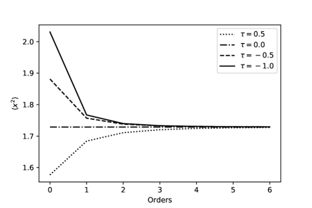
Figure 1: Dependence of $I$ on the number of CS terms at different $\tau$.

The decrease of the curves at $\tau<0$ indicates the presence of negative terms in CS.

Despite that in the considered example the CS terms lose their positivity due to the change of $\tau=0$ to $\tau=-1$ or to $\tau=-1/2$, one can note that the series nevertheless converges to the correct answer. In the work [3] it is explained by employing an additional regularization of the form

$$I = \lim_{\gamma\rightarrow 0}I(\gamma)\,,$$ (16)

$$I(\gamma) := \int_{-\infty}^{\infty}dx\,e^{-S[x]}e^{-\gamma S_{2}^{3}[x]}\,,$$ (17)

where the notations $S[x]:=\frac{1}{2}m^{2}x^{2}+\frac{\lambda}{4!}x^{4}$ and $S_{2}[x]:=\frac{1}{2}m^{2}x^{2}$ are used to emphasize the analogy with lattice models. The representation (16) is always correct for the finite dimensional integrals, i.e. there is always such $\gamma_{*}$, that $I(\gamma_{*})$ approximates $I(\gamma)$ with an arbitrary precision. At $\gamma>0$ the application of the CS method for computing $I(\gamma>0)$ generates the convergent series even at $\tau\neq 0$. The latter can be proved by considering the large order asymptotic of the perturbative re-expansion of the CS representation for $I(\gamma>0)$.

In case of the infinite dimensional integrals, the $\gamma$-regularization (16), (17) is not valid. It happens because the term analogous to $\gamma S_{2}^{3}[x]$ is non-local and the models with local and non-local actions have different scalings at $V\rightarrow\infty$. Nevertheless, note that the failure of the regularization (16), (17) prohibits the proof from [3] for infinite volumes, but does not necessary imply the inapplicability of the CS method. Here we study numerically the workability of the CS method investigating the $\phi^{4}$-model defined on the one- and two-dimensional infinite lattices. Then, we prove the correctness of the results by showing that the Borel summability is a sufficient condition for the CS applicability.

3 Convergent series for the lattice $\phi^{4}$-model

The discretized version of the action (2) (now in an arbitrary dimension $D$) is given by

$$S_{E}=S_{2}[\varphi]+S_{4}[\varphi]\,,$$ (20)

$$S_{2}[\varphi]=-\frac{1}{2}\sum_{n,\mu}\varphi_{n}\varphi_{n+\mu}+\frac{1}{2}(2D+M^{2})\sum_{n}\varphi_{n}^{2}\,,$$

$$S_{4}[\varphi]=\frac{\lambda}{4!}\sum_{n}\varphi_{n}^{4},$$

where $\varphi=a\phi$, $M=am$, $x=na$, $\int d^{D}x\to a^{D}\sum_{n}$, $(\partial_{\mu}\phi)^{2}\to\frac{1}{a^{2}}\sum_{\mu}(2\phi(na)-\phi(na+\mu a)-\phi(na-\mu a))$, $n$ is the $D$-dimensional integer vector, $\mu$ is the unit vector directed along the $\mu$-axis, $a$ is the lattice spacing. This action leads to the standard perturbation theory with tetravalent vertices and a bare propagator given by

$$\langle\varphi_{n}\varphi_{m}\rangle_{0}=\int_{-\pi}^{\pi}\frac{d^{D}k}{(2\pi)^{D}}\frac{e^{ik(n-m)}}{4\sum_{\mu}\sin^{2}\frac{k_{\mu}}{2}+M^{2}}.$$ (21)

The CS expression for the two-point function of the $\phi^{4}$-model on the lattice of the size $V$ is derived in a complete analogy to (12)

$$\langle\varphi_{n}\varphi_{m}\rangle_{\lambda} = \sum_{k=0}^{\infty}\frac{1}{k!}\int_{0}^{\infty}\,dt\,t^{V+\tau+4k+1}\exp\Bigl{(}-t^{2}-\sigma t^{4}\Bigr{)}$$ (22)

$$\cdot\sum_{l=0}^{k}\binom{k}{l}\sigma^{k-l}\frac{2f_{l}(n,m)\lambda^{l}}{\Gamma\Bigl{(}\frac{V+\tau+4l+2}{2}\Bigr{)}},$$

where $f_{l}(n,m)/(l!)$ are the coefficients of the standard perturbation theory, i.e. $\langle\varphi_{n}\varphi_{m}\rangle_{\lambda}\sim\sum_{l=0}^{\infty}f_{l}(n,m)/(l!)\lambda^{l}$ and $\sigma$ is the parameter of the new initial approximation, we choose it to be the minimal $\sigma$ satisfying the inequality (5),

$$\sigma=\frac{\lambda}{6M^{4}}\,.$$ (23)

We apply (22) to the limiting case $V+\tau=0$, $V\rightarrow\infty$ and compare the results with corresponding extrapolations of the path integral Monte Carlo (PIMC) simulations data and the Borel re-summation of the standard perturbation theory.

4 Numerical results

The main building blocks of the CS are the terms of the standard perturbation theory. Their computations in the infinite volume limit are much simpler than for finite lattices. At finite lattice volumes, an evaluation of each diagram of the $\phi^{4}$-model involves the multiplication of $4$ bare-propagator matrices of the size $V\times V$ per vertex leading to the enormously long computations. However, by turning to the computations in the infinite volume limit, one substitutes tedious matrix multiplications by numerical integrations, which can be performed with the Monte Carlo technique.

On the Fig. 2 we present the $\langle\varphi_{n}^{2}\rangle$-operator of the one-dimensional lattice $\phi^{4}$-model depending on the number of computed terms of the standard perturbation theory at two reference values of the coupling constant, $\lambda=1$ and $\lambda=10$. All plots exhibit that the CS method converges to the extrapolated Monte Carlo answer faster than the Borel re-summation procedure (for the details of the PIMC computations and Borel re-summation see Appendix A).

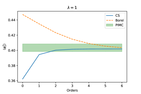
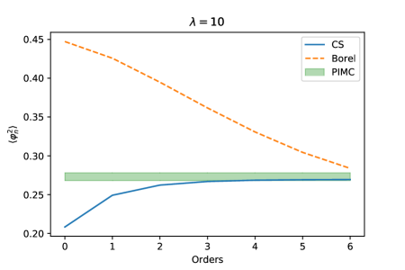
Figure 2: Dependence of $\langle\varphi_{n}^{2}\rangle$ computed with the CS method and Borel re-summation on the number of series terms and comparison with the extrapolated PIMC data, $D=1$, at $\lambda=1$ and $\lambda=10$.

In Fig. 3 we show the coupling constant dependence of the $\langle\varphi_{n}^{2}\rangle$-operator computed with six orders of the CS and Borel series. The reference ’correct’ answer is obtained by the extrapolation of the PIMC computations. The CS method demonstrates better precision at large values of the coupling constant than Borel re-summation.

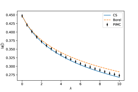
Figure 3: Dependence on the coupling constant of the $\langle\varphi_{n}^{2}\rangle$-operator computed with the sixth order of the CS and Borel series and PIMC extrapolation, $D=1$.

The consideration of the two-dimensional infinite lattice demonstrates similar results. On the Fig. 4 we present the results for the $\langle\varphi_{n}^{2}\rangle$-operator depending on the number of computed terms of the standard perturbation theory at $\lambda=1$ and $\lambda=10$.

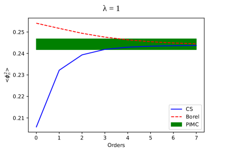
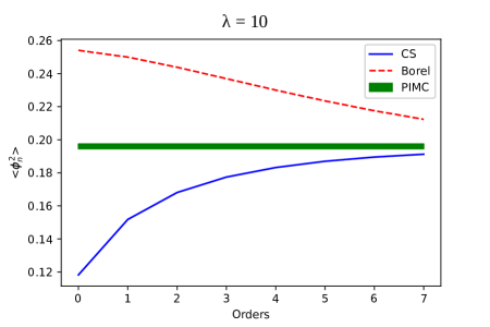
Figure 4: Dependence of $\langle\varphi_{n}^{2}\rangle$ computed with the CS method and Borel re-summation on the number of series terms and comparison with the extrapolated PIMC data, $D=2$, at $\lambda=1$ and $\lambda=10$.

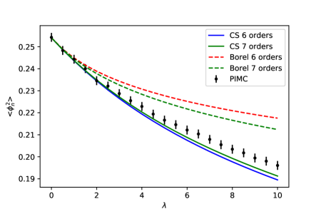
Figure 5: $\langle\varphi_{n}^{2}\rangle$-operator depending on the coupling constant computed with the sixth and seventh orders of the CS and Borel series and PIMC extrapolation, $D=2$.

In Fig. 5 we show the value of the $\langle\varphi_{n}^{2}\rangle$-operator depending on the coupling constant, emphasizing the improvement achieved by going from the sixth order approximation to the seventh.

5 Relation to the Borel summability

The remarkable workability of the CS method for finite lattices was explained in [3] by considering a $\phi^{4}$-model regularized by an additional non-local interaction with a vanishing coupling. As it was mentioned in the Section 2, such approach can not be used for the infinite lattices, since the regularization used in [3] adds a non-local term to the action. Models with non-local interactions have an unusual (different from ones with a local interaction) scaling with respect to the lattice volume. Consequently, non-local models never approximate local ones in the limit of the infinite amount of d. o. f. Nevertheless, we use the regularization of the $\phi^{4}$-model of the type of [3] just as a motivation for an another construction, providing a link between the applicability of the CS method for infinite lattices and the Borel summability.

Let us consider a model, defined on the infinite lattice by the action

$$S_{\gamma}=S_{2}[\varphi]+S_{4}[\varphi]+\gamma(S_{2}[\varphi])^{3},$$ (24)

where $S_{2}[\varphi]$ and $S_{4}[\varphi]$ are given by (4) and (20) respectively and $\gamma\geq 0$ is a parameter. For this model one can write a formal expression analogous to (12)

$$Z_{\gamma}=\frac{1}{Z_{0}}\sum_{k}\frac{1}{k!}\int_{0}^{\infty}dt\,t^{V+4k-1}\,e^{-t^{2}-\sigma t^{4}-\gamma t^{6}}\sum_{l=0}^{k}\binom{k}{l}\frac{\sigma^{k-l}f_{l}}{\Gamma\Big{(}\frac{V+4l}{2}\Big{)}}\,.$$ (25)

The equation (25) is ill defined when $V\rightarrow\infty$. However, as it was shon in [3], at $\gamma=0$ for any $V$, there is an invariance (at least perturbative) allowing one to substitute $V$ by $V+\tau=w$, where $w$ is finite. In case of finite lattices [3], the continuity of $Z_{\gamma}$ at $\gamma\rightarrow 0$ was used for justifying the change from $V$ to $V+\tau=w$ in the non-perturbative sense. Since limits $V\rightarrow\infty$ and $\gamma\rightarrow 0$ do not commute, we cannot follow the same way. Instead of thinking about the regularization of the model, we just consider the series (25). We do not perform the limit $V\rightarrow\infty$. Instead, we do a formal substitution $V-->w$ (as it is prescribed by the CS method) and prove that it leads to the correct answer, independently on $V$, if $Z$ is Borel-summable. Indeed, considering the asymptotic of large orders [3], one can show that for $\gamma>0$ the series

$$Z_{\gamma}^{w}:=\frac{1}{Z_{0}}\sum_{k}\frac{1}{k!}\int_{0}^{\infty}dt\,t^{w+4k-1}\,e^{-t^{2}-\sigma t^{4}-\gamma t^{6}}\sum_{l=0}^{k}\binom{k}{l}\frac{\sigma^{k-l}f_{l}}{\Gamma\Big{(}\frac{w+4l}{2}\Big{)}}\,.$$ (26)

is absolutely convergent. The re-expansion (re-summation) of (26) in the coupling constant $g$ generates an another absolutely convergent series for $Z_{\gamma}^{w}$,

$$Z_{\gamma}^{w} = \frac{1}{Z_{0}}\sum_{l=0}^{\infty}\frac{1}{l!}\int_{0}^{\infty}dt\,t^{w+4l-1}\,e^{-t^{2}-\gamma t^{6}}\frac{f_{l}}{\Gamma\Big{(}\frac{w+4l}{2}\Big{)}}\,.$$ (27)

The equivalence of (26) and (27) is guarantied by their absolute convergence. Due to the absolute convergence, one can interchange the summation and integration in (27)

$$Z_{\gamma}^{w} = \frac{1}{Z_{0}}\int_{0}^{\infty}dt\,t^{w-1}\,e^{-t^{2}-\gamma t^{6}}\sum_{l=0}^{\infty}\frac{t^{4l}f_{l}/(l!)}{\Gamma\Big{(}\frac{w+4l}{2}\Big{)}}\,,$$ (28)

where $f_{l}/(l!)$ are the coefficients of the standard perturbation theory. At $\gamma=0$ the expression (28) is nothing more than the Borel-Leroy summation of the SPT series for $Z$. Then, the possibility to take the limit $\gamma\rightarrow 0$ (or in other words to use CS method for the infinite lattices) follows from the Borel summability.

6 Concluding remarks

In this paper we have studied the applicability of the convergent series to the systems with an infinite amount of degrees of freedom. Considering $\phi^{4}$-model on the one and two-dimensional infinite lattices, we have provided a numerical evidence of the robustness of the CS method. Our computations indicate, that the convergent series approaches to the reference Monte Carlo results (where an infinite lattice volume is reached by an extrapolation procedure) faster than the corresponding Borel summation.

For a long time (starting from the first papers in the 1980s [2, 11, 12]) the derivation of the method was based on the utilization of the dimensional regularization and the justification of the CS method for the infinite systems was remaining an open question. Here we have shown that the utilization of the dimensional regularization is equivalent to an additional re-summation procedure. We have proved that this additional re-summation preserves the convergence of the CS method if the model is Borel summable. The Borel summability is a sufficient condition for the correctness of the CS method in the limit of an infinite amount of degrees of freedom. It is not hard to find an effective action, satisfying the inequality analogous to (5) even in case of some Borel non-summable models, for instance, for the double-well potential. Then, the logic of the paper [3] suggests, that on the finite lattices the CS method should be correct also for the models which are Borel non-summable. Taking into account results of the current paper, one can hope that the CS method is applicable to a wider class of the quantum field theories than the Borel re-summation and can serve as a new tool for the analytic non-perturbative computations.

Acknowledgments

The work of AI was supported by the Foundation for the Advancement of Theoretical Physics “BASIS” 17-21-103-1 and by Russian Science Foundation Grant No. 14-22-00161. VS acknowledges the support provided by the Austrian Science Fund (FWF) trough the Erwin Schrödinger fellowship J-3981.

Appendix A

A.1 Borel re-summation

To perform the Borel re-summation procedure, we use the conformal mapping [20] for the analytic continuation in the Borel plane. The conformal mapping can be done if the parameter $a$ from the asymptotic of the high orders of the perturbation theory,

$$\frac{f_{k}}{k!}\sim(-1)^{k}\sqrt{2\pi}e\big{(}\frac{a}{e}\big{)}^{k}k^{k+b_{0}+1/2}\,,$$ (29)

is known. We estimate $a$ using the values presented in [21] for the continuous one- and two-dimensional $\phi^{4}$-model

$$d=1\,,~{}~{}~{}a=1/8\,,$$ (30)

$$d=2\,,~{}~{}~{}a=1/35.102\,...\,.$$ (31)

A.2 PIMC

To approach the infinite volume results using the PIMC method we analyze lattices of diferent sizes, see Fig. 6 and 7. We assume that the infinite volume limit is achieved at the lattices with the volume $V=10000$ in the one dimensional case and $V=64\times 64$ in two dimensions.

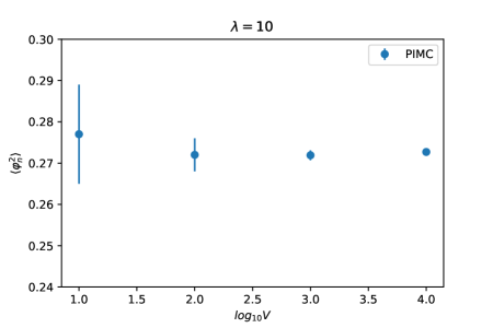
Figure 6: Infinite volume limit in the PIMC computations, $D=1$.

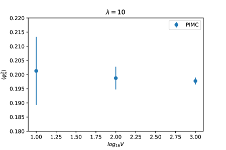
Figure 7: Infinite volume limit in the PIMC computations, $D=2$.

References

- [1] I. G. Halliday and P. Suranyi. Anharmonic oscillator: A new approach. Phys. Rev. D, 21:1529–1537, Mar 1980.
- [2] A. G. Ushveridze. Converging perturbational scheme for the field theory. (in Russian). Yad. Fiz., 38:798–809, 1983.
- [3] Aleksandr S. Ivanov and Vasily K. Sazonov. Convergent series for lattice models with polynomial interactions. Nuclear Physics B, 914:43 – 61, 2017.
- [4] Vasily Sazonov. Convergent series for polynomial lattice models with complex actions. arXiv:1706.03957 [hep-lat], 2017.
- [5] Y. Meurice. Simple method to make asymptotic series of Feynman diagrams converge. Phys. Rev. Lett., 88:141601, Mar 2002.
- [6] B. Kessler, L. Li, and Y. Meurice. New optimization methods for converging perturbative series with a field cutoff. Phys. Rev. D, 69:045014, Feb 2004.
- [7] V.V. Belokurov, Yu.P. Solov’ev, and E.T. Shavgulidze. Method of approximate evaluation of path integrals using perturbation theory with convergent series. i. Theoretical and Mathematical Physics, 109(1):1287–1293, 1996.
- [8] V. K. Sazonov. Convergent perturbation theory for lattice models with fermions. International Journal of Modern Physics A, 31(13):1650072, 2016.
- [9] Vincent Rivasseau and Zhituo Wang. How to resum Feynman graphs. Annales Henri Poincare, 15(11):2069–2083, 2014.
- [10] Thomas Krajewski, Vincent Rivasseau, and Vasily Sazonov. Constructive matrix theory for higher order interaction. arXiv:1712.05670 [math-ph], December 2017.
- [11] B.S. Shaverdyan and A.G. Ushveridze. Convergent perturbation theory for the scalar field theories; the gell-mann-low function. Physics Letters B, 123(5):316 – 318, 1983.
- [12] A.G. Ushveridze. Superconvergent perturbation theory for euclidean scalar field theories. Physics Letters B, 142(5-6):403 – 406, 1984.
- [13] A. V. Turbiner and A. G. Ushveridze. Anharmonic oscillator: Constructing the strong coupling expansions. Journal of Mathematical Physics, 29(9), 1988.
- [14] A.N. Sissakian, I.L. Solovtsov, and O.Yu. Shevchenko. Convergent series in variational perturbation theory. Physics Letters B, 297(3):305 – 308, 1992.
- [15] A. N. Sisakian and I. L. Solovtsov. Variational perturbation theory: Anharmonic oscillator. Z. Phys., C54:263–271, 1992.
- [16] Juha Honkonen and Mikhail Nalimov. Convergent expansion for critical exponents in the -symmetric model for large . Physics Letters B, 459(4):582 – 588, 1999.
- [17] George Leibbrandt. Introduction to the technique of dimensional regularization. Rev. Mod. Phys., 47:849–876, Oct 1975.
- [18] V.V. Belokurov, A.S. Ivanov, V.K. Sazonov, and E.T. Shavgulidze. Convergent perturbation theory for the lattice -model. PoS Lattice2015, arXiv:1511.05959, 2015.
- [19] Giorgio Talenti. Best constant in sobolev inequality. Annali di Matematica Pura ed Applicata, 110(1):353–372, 1976.
- [20] J. C. Le Guillou and J. Zinn-Justin. Critical exponents for the -vector model in three dimensions from field theory. Phys. Rev. Lett., 39:95–98, Jul 1977.
- [21] Jean Zinn-Justin and Ulrich D. Jentschura. Order-dependent mappings: Strong-coupling behavior from weak-coupling expansions in non-hermitian theories. Journal of Mathematical Physics, 51(7):072106, 2010.