Particle Swarm Optimization based search for gravitational waves from compact binary coalescences: performance improvements

Abstract

While a fully-coherent all-sky search is known to be optimal for detecting signals from compact binary coalescences (CBCs), its high computational cost has limited current searches to less sensitive coincidence-based schemes. For a network of first generation GW detectors, it has been demonstrated that Particle Swarm Optimization (PSO) can reduce the computational cost of this search, in terms of the number of likelihood evaluations, by a factor of $\approx 10$ compared to a grid-based optimizer. Here, we extend the PSO-based search to a network of second generation detectors and present further substantial improvements in its performance by adopting the local-best variant of PSO and an effective strategy for tuning its configuration parameters. It is shown that a PSO-based search is viable over the entire binary mass range relevant to second generation detectors at realistic signal strengths.

I Introduction

The advanced Laser Interferometric Gravitational-wave Observatory (LIGO) Abbott et al. (2016) and the Advanced Virgo Acernese et al. (2015) detectors have detected gravitational waves (GWs) from several compact binary coalescence (CBC) events over their recently concluded observation runs. Among the detected signals, GW150914 Abbott et al. (2016a), GW151226 Abbott et al. (2016b), and GW170104 Abbott et al. (2017a) are binary black hole (BBH) mergers detected in two-way coincidence between the LIGO detectors, while GW170814 Abbott et al. (2017b) is a BBH merger detected in three-way coincidence after Virgo joined the LIGO observation runs. GW170817 Abbott et al. (2017c), the final event in the last observing run, was a binary neutron star (BNS) inspiral. Its prompt localization on the sky by the LIGO-Virgo network allowed the detection of an electromagnetic (EM) counterpart Abbott et al. (2017d), establishing BNS mergers as the source of some short gamma-ray bursts.

Over the next few years, LIGO and Virgo will be joined by the KAGRA Somiya (2012) detector in Japan and LIGO-India Unnikrishnan (2013). Combining the data from this network of geographically distributed second generation detectors will significantly increase both the detection sensitivity and sky localization of CBC sources Fairhurst (2009); Nissanke et al. (2011).

It is known that the optimal data analysis methods for the detection and estimation of CBC signals with a network of GW detectors are the Generalized Likelihood Ratio Test (GLRT) and Maximum Likelihood Estimation (MLE) respectively Kay (1993). In the GW literature, the GLRT is called the fully coherent all-sky search. (For a single detector, the GLRT is the matched filter Helstrom (1968).)

In both GLRT and MLE, the joint likelihood function of data from a network of detectors needs to be maximized over the space of CBC signal parameters. However, the computational cost of this task has proven to be a limiting factor in running the GLRT as an always-on search. The difficulty of the optimization stems from a combination of (i) the high dimensionality of the search space, and (ii) the high computational cost of evaluating the likelihood at a given point in the search space. The latter is due to the requirement of correlating pairs of time series that involve $O(10^{6})$ samples each (for low binary component masses).

To circumvent the computational bottleneck above, current CBC searches use a coincidence-based semi-coherent approach in which the GLRT is only used when (i) computationally cheaper single-detector matched filter searches result in the crossing of preset detection thresholds in any pair of detectors, and (ii) the corresponding estimated signal parameters are proximal within some preset tolerances. As shown in Macleod et al. (2016), a semi-coherent search trades-off a significant amount of sensitivity for the reduced computational cost, with the detection volume being $\sim 25\%$ smaller than a fully-coherent search.

It has recently been demonstrated in (Weerathunga and Mohanty, 2017), henceforth referred to as WM, that Particle Swarm Optimization (PSO) (Kennedy and Eberhart, 1995), a family of stochastic global optimization methods based on the behavior of biological swarms, can potentially solve this challenge. Simulation of a four detector network, coinciding with the location and orientation of the LIGO Hanford (H), LIGO Livingston (L), Virgo (V), and KAGRA (K), showed that the number of likelihood evaluations required by PSO is $\sim 1/10$ that of a grid-based search in which the search space is populated densely with a fixed set of sampling locations.

The results in WM were derived under the following limitations. (i) It was assumed that the noise in each detector had a Power Spectral Density (PSD) given by the initial LIGO design sensitivity curve Albert Lazzarini (1996). This was primarily done to keep signal lengths short ($\lesssim 30$ sec) and the computational run time manageable given the matlab mat based implementation of the search. (ii) As with any stochastic optimization algorithm, PSO is not guaranteed to converge to the global optimum. For the so-called global-best variant of PSO used in WM, this led to a small but non-zero reduction in detection probability of $\lesssim 2.5\%$. (iii) A PSO-based search can be parallelized efficiently in a multi-processor environment but the code did not implement all of the possible layers of parallelization.

In this paper, we develop the PSO-based fully-coherent all-sky search further by overcoming the above limitations. (i) We shift to the advanced LIGO design sensitivity and examine the performance of PSO for both short ($O(1)$ min) and long ($O(30)$ min) data lengths. (ii) We use the local-best variant of PSO and find it to be significantly better in terms of convergence, achieving $\lesssim 0.5\%$ loss in detection probability for $\approx 1$ min long data at lower signal strengths than the one used in WM. (iii) Besides translating the code into the C language, a two-layered parallelization scheme is implemented that speeds up execution by a factor of $\approx 7.5$.

The rest of the paper is organized as follows. Sec II sets up the data model used in this paper and provides pertinent details of the fully-coherent all-sky search. Sec. III describes the local best PSO algorithm and a general purpose strategy for tuning its performance on parametric GW data analysis problems. The simulation setup and results on detection and estimation performance of the PSO-based search are presented in Sec. IV. The computation time of the current code is discussed in Sec. V along with possible future avenues that could reduce it substantially. The conclusions from our study are presented in Sec  VI.

II Fully-coherent all-sky search

While the review of the data model and the fully-coherent all-sky search in this section provides a self-contained background for the rest of the paper, we refer the reader to WM and references therein for a comprehensive presentation of mathematical details.

II.1 Data and Signal Models

Consider the ${i}^{\rm th}$ detector in a network of $D$ detectors. A segment of the strain time series recorded by the detector is given by

$$x^{i}(t)=\left\{\begin{array}[]{lc}n^{i}(t);&H_{0},\\ h^{i}(t)+n^{i}(t);&H_{1}\end{array}\right.$$ (1)

where $h^{i}(t)$ is the detector response to the incident GW and $n^{i}(t)$ denotes detector noise. $H_{0}$ and $H_{1}$ correspond to the two hypotheses one can propose about the data where a signal is, respectively, absent or present.

We will assume that $n^{i}(t)$ is a realization of a zero-mean, stationary Gaussian stochastic process,

$$E[n^{i}(t)] = 0;$$ (2)

$$E[n^{i}(t)n^{i}(t^{\prime})] = \frac{1}{2}\int_{-\infty}^{\infty}dfe^{2\pi jf(t-t^{\prime})}S_{n}(f)\;,$$ (3)

with $S_{n}(f)$ denoting the one-sided noise power spectral density (PSD). It does not carry a detector index in this paper because we assume identical PSD for all the detectors.

For a source located at azimuthal angle $\alpha$ and polar angle $\delta$ in the Earth Centered Earth Fixed Frame (ECEF) Alfred Leick (2004), the detector responses are given by,

$$\left(\begin{array}[]{c}h^{1}(t+\Delta^{1}(\alpha,\delta))\\ h^{2}(t+\Delta^{2}(\alpha,\delta))\\ \vdots\\ h^{D}(t+\Delta^{D}(\alpha,\delta))\end{array}\right) = {\bf F}(\alpha,\delta,\psi)\left(\begin{array}[]{c}h_{+}(t)\\ h_{\times}(t)\end{array}\right)\;,$$ (10)

where the ${i}^{\rm th}$ row of the antenna pattern matrix ${\bf F}(\alpha,\delta,\psi)$ contains the antenna pattern functions $(F_{+}^{i}(\alpha,\delta,\psi),\;F_{\times}^{i}(\alpha,\delta,\psi))$ of the ${i}^{\rm th}$ detector, $h_{+}(t)$ and $h_{\times}(t)$ are the TT gauge polarization components of the GW plane wave incident on the origin of the ECEF, and $\Delta^{i}(\alpha,\delta)$ is the time delay between the plane wave hitting the ECEF origin and the ${i}^{\rm th}$ detector. The polarization angle $\psi$ gives the orientation of the wave frame axes with respect to the fiducial basis formed by $-\widehat{\alpha}$ and $\widehat{\delta}$ in the plane orthogonal to the wave propagation direction.

The condition number Rakhmanov (2006) of the antenna pattern matrix as a function of $\alpha$ and $\delta$ plays an important role in determining the errors in the estimation of the source location Wang and Mohanty (2017). In general, the errors worsen as the condition number at the source location increases. However, as will be apparent in Sec. IV.3, the influence of the condition number is more subtle than this empirical rule of thumb.

In this paper, we use a four-detector network consisting of the two LIGO detectors at Hanford (H) and Livingston (L), Virgo (V) and KAGRA (K). For simplicity, we assume the advanced LIGO design PSD Shoemaker (2010) corresponding to the “ZERO DET high P” configuration for the noise in each detector. The orientations and locations of the detectors, listed in table II of WM, match their real-world values. A sky map of the condition number of the antenna pattern matrix for the above detector network is shown in Figure 4 of WM.

The polarizations $h_{+}(t)$ and $h_{\times}(t)$ used in this paper are given by the restricted 2-PN waveform from a circularized binary consisting of non-spinning compact objects Blanchet et al. (1995) that depends on the following parameters. (i) The component masses $m_{1}$ and $m_{2}$ expressed through the chirp times $\tau_{0}$ and $\tau_{1.5}$,

$$\tau_{0} = \frac{5}{256\pi}f_{*}^{-1}\left(\frac{GM}{c^{3}}\pi f_{*}\right)^{-5/3}\eta^{-1}\;,$$ (11)

$$\tau_{1.5} = \frac{1}{8}f_{*}^{-1}\left(\frac{GM}{c^{3}}\pi f_{*}\right)^{-2/3}\eta^{-1}\;,$$ (12)

$$M = m_{1}+m_{2}\;,\quad\mu=\frac{m_{1}m_{2}}{M}\;,\quad\eta=\frac{\mu}{M}\;,$$ (13)

where $f_{*}$, set to $10$ Hz in this paper, is the lower cutoff frequency of the detector arising from the steep rise in seismic noise. (ii) The time $t_{c}$ at which the end of the inspiral signal arrives at the ECEF origin. (iii) The phase of the signal at $t_{c}$ given by $\phi_{c}$. (iv) The overall amplitude of the signal denoted by $A$. The duration of the signal starting from the time at which its instantaneous frequency equals $f_{\ast}$ to $t_{c}$ is given by $\tau_{0}+\tau_{1}-\tau_{1.5}+\tau_{2}$ where,

$$\tau_{1} = \frac{5}{192\pi}f_{*}^{-1}\left(\frac{GM}{c^{3}}\pi f_{*}\right)^{-1}\eta^{-1}\left(\frac{743}{336}+\frac{11}{4}\eta\right)\;,$$ (14)

$$\tau_{2} = \frac{5}{128\pi}f_{*}^{-1}\left(\frac{GM}{c^{3}}\pi f_{*}\right)^{-1/3}$$ (15)

$$\eta^{-1}\left(\frac{3058673}{1016064}+\frac{5429}{1008}\eta+\frac{617}{144}\eta^{2}\right)\;,$$

are additional chirp times for the 2PN waveform.

II.2 Likelihood ratio for a detector network

Under our assumption of Gaussian, stationary noise, the log-likelihood Ratio (LLR) Helstrom (1995) for the ${i}^{\rm th}$ detector is given by,

$${\rm ln}\;\lambda^{{i}} = {\langle}x^{i}|h^{i}{\rangle}-\frac{1}{2}{\langle}h^{i}|h^{i}{\rangle}\;,$$ (16)

where, with $\widetilde{a}(f)$ denoting the Fourier transform of any function $a(t)$ of time,

$${\langle}\;p\;|\;q\;{\rangle} = 4\;{\rm Re}\int_{0}^{\infty}df\;\frac{\widetilde{p}(f)\widetilde{q}^{\ast}(f)}{{S_{n}}(f)}\;.$$ (17)

If we assume the noise in different detectors to be statistically independent, the log-likelihood for a $D$ detector network is given by,

$$\rm{ln}\;\lambda = \sum_{i=1}^{D}\left[{\langle}x^{i}|h^{i}{\rangle}-\frac{1}{2}{\langle}h^{i}|h^{i}{\rangle}\right]\;.$$ (18)

It follows that, for a given data realization, the log-likelihood is a function of the parameters $\theta=\{\tau_{0},\tau_{1.5},\alpha,\delta,t_{c}\}$, $A$, $\psi$, and $\phi_{c}$.

The GLRT statistic is the global maximum of the LLR over the parameters mentioned above. Adopting the notation in Bose et al. (2011), we use the equivalent of the GLRT statistic defined as

$$\rho_{\rm coh}^{2} = 2\max_{A,\psi,\phi_{c},\theta}\ln\lambda\;,$$ (19)

and call $\rho_{\rm coh}$ the coherent search statistic.

The Maximization can be carried out as,

$$\rho_{\rm coh}^{2} = \max_{\theta}\gamma^{2}(\theta)\;,$$ (20)

$$\gamma^{2}(\theta) = 2\max_{A,\psi,\phi_{c}}\ln\lambda\;.$$ (21)

The inner maximization can be performed analytically, while the outer maximization over $\theta$ must be carried out numerically.

For fixed $\{\tau_{0},\tau_{1.5},\alpha,\delta\}$, the maximization over $t_{c}$ can be carried out very efficiently using the Fast Fourier Transform (FFT) Bose et al. (2011). The FFT-based approach is made especially convenient by the fact that the polarization waveforms can be generated directly in the Fourier domain using the stationary phase approximation Sathyaprakash and Dhurandhar (1991). Thus, the outer maximization can be further split over $\Theta=\{\tau_{0},\tau_{1.5},\alpha,\delta\}$ and $t_{c}$. We call

$$\Gamma^{2}(\Theta) = \max_{t_{c}}\gamma^{2}(\theta)\;\Rightarrow\;\rho^{2}_{\rm coh}=\max_{\Theta}\Gamma^{2}(\Theta),$$ (22)

the coherent fitness function. The computational cost of maximizing the coherent fitness over $\Theta$ is the main challenge in the implementation of a fully coherent search.

In any practical implementation of the fully-coherent all-sky search, the data streams from GW detectors must be analyzed in finite length segments. Consequently, for fixed $\Theta$, $\gamma^{2}(\theta)$ is not valid for $t_{c}$ greater than the length of the segment being analyzed. However, the FFT-based calculation generates $\gamma^{2}(\theta)$ for $t_{c}$ going up to the sum of the segment length and the length of the signal corresponding to $\Theta$. To account for this effect, the spurious values of $\gamma^{2}(\theta)$ are deleted and consecutive data segments are overlapped by at least the length of the signal. In this paper, we analyze simulated data realizations that are generated independently of each other. Hence, there is no need to overlap them. However, care is taken to ensure that the signal embedded in the data has a $t_{c}$ that is sufficiently small. As long as the estimated $t_{c}$ does not stray too far from its true value, which was verified to be the case in our simulations, ignoring deletion and overlapping does not affect our results.

III Particle Swarm Optimization

Although PSO started off as a single algorithm, the term now refers to a diverse set of algorithms and it is viewed more properly as a metaheuristic – a general approach to optimization based on a particular type of physical or biological model. In the case of PSO, the model happens to be the flocking or swarming behavior of biological agents (birds, fish etc.). In fact, the PSO metaheuristic is one among many others that are inspired by nature.

PSO uses a fixed number of samples (called particles) of the function to be optimized (called the fitness function). The particles move in the search space following stochastic iterative rules called the dynamical equations. In WM, the PSO algorithm used was the global-best (or gbest) variant. In this paper, we use the local-best (or lbest) variant of PSO described below that leads to a significantly improved performance.

III.1 The lbest PSO algorithm

We adopt the following notation in this section for describing lbest PSO.

• $f(x)$: the scalar fitness function to be maximized, with $x=(x^{1},x^{2},\ldots,x^{d})\in\mathbb{R}^{d}$. In our case, $x=\Theta$, $f(x)$ is the coherent fitness function $\Gamma^{2}(\Theta)$ (c.f., Eq. 22) and $d=4$.

• $\mathcal{S}\subset\mathbb{R}^{d}$: the search space defined by the hypercube $a^{i}\leq x^{i}\leq b^{i}$, $i=1,2,\ldots,d$. Among a set of locations in $\mathcal{S}$, the best location is the one with the maximum fitness.

• $N_{p}$: the number of particles in the swarm.

• $x_{i}[k]$: the position of the $i^{\rm th}$ particle at the $k^{\rm th}$ iteration.

• $p_{i}[k]$: the best location found by the $i^{\rm th}$ particle over all iterations up to and including the $k^{\rm th}$. $p_{i}[k]$ is called the personal best position of the $i^{\rm th}$ particle.

  $$f(p_{i}[k]) = \max_{j\leq k}f(x_{i}[j])\;.$$ (23)

• $n_{i}[k]$: a set of particles, called the nearest neighbors of particle $i$, $n_{i}[k]\subseteq\{1,2,\ldots,N_{p}\}\setminus\{i\}$. There are many possibilities, called topologies, for the choice of $n_{i}[k]$. In this paper, we use the ring topology with $2$ neighbors in which

  $$n_{i}[k]=\left\{\begin{array}[]{cc}\{i-1,i+1\}\;,&i\notin\{1,N_{p}\}\\ \{N_{p},i+1\}\;,&i=1\\ \{i-1,1\}\;,&i=N_{p}\end{array}\right.\;.$$ (27)

• $l_{i}[k]$: the best location among the particles in $n_{i}[k]$. $l_{i}[k]$ is called the local best position of the $i^{\rm th}$ particle.

  $$f(l_{i}[k]) = \max_{j\in\{i\}\cup n_{i}[k]}f(x_{j}[k])\;.$$ (28)

• $p_{g}[k]$: The best location among all the particles over all iterations up to and including the $k^{\rm th}$.

  $$f(p_{g}[k]) = \max_{1\leq j\leq N_{p}}f(x_{j})\;.$$ (29)

The dynamical equations for lbest PSO are as follows.

$$v_{i}[k+1] = w[k]v_{i}[k]+c_{1}{\bf r}_{1}(p_{i}[k]-x_{i}[k])+$$ (30)

$$c_{2}{\bf r}_{2}(l_{i}[k]-x_{i}[k])\;.$$

$$x_{i}[k+1] = x_{i}[k]+z_{i}[k+1]\;,$$ (31)

$$z^{j}_{i}[k] = \left\{\begin{array}[]{cc}v_{i}^{j}[k],&-v_{\rm max}^{j}\leq v_{i}^{j}[k]\leq v_{\rm max}^{j}\\ -v_{\rm max}^{j},&v_{i}^{j}[k]<-v_{\rm max}^{j}\\ v_{\rm max}^{j}&v_{i}^{j}[k]>v_{\rm max}^{j}\end{array}\right.\;,$$ (35)

Here, $v_{i}[k]$ is called the “velocity” of the $i^{\rm th}$ particle, $w[k]$ is a deterministic function known as the inertia weight (see below), $c_{1}$ and $c_{2}$ are constants, and ${\bf r}_{i}$ is a diagonal matrix with independent, identically distributed random variables having a uniform distribution over $[0,1]$. The second and third terms on the RHS of Eq. 30 are called the cognitive and social terms respectively.

The iterations are initialized at $k=1$ by independently drawing (i) $x_{i}^{j}[1]$ from a uniform distribution over $[a^{j},b^{j}]$, and (ii) $v_{i}^{j}[1]$ from a uniform distribution over $[-v_{\rm max}^{j},v_{\rm max}^{j}]$. The algorithm terminates when the number of iterations reaches a prescribed number ${N_{\rm iter}}$. The solutions to the maximizer and maximum value of the fitness found by PSO are $p_{g}[N_{\rm iter}]$ and $f(p_{g}[N_{\rm iter}])$ respectively.

To handle particles that exit the search space, we use the “let them fly” boundary condition under which a particle outside the search space is assigned a fitness values of $-\infty$. Since both $p_{i}[k]$ and $l_{i}[k]$ are always within the search space, such a particle is eventually dragged back into the search space by the cognitive and social terms.

The role of the inertia weight, $w[k]$, is to control the degree of exploration of the search space by allowing a particle to overcome the attractive cognitive and social terms. In the version of PSO used here, the inertia weight $w[k]$ decreases linearly with $k$ from an initial value $w_{\rm max}$ to a final value $w_{\rm min}$. Decreasing the inertia weight transitions PSO from an initially exploratory to a final exploitative phase, and the longer the interval, namely $N_{\rm iter}$, over which this happens, the later the onset of the transition.

III.2 PSO tuning metric

As mentioned earlier, PSO is not guaranteed to converge to the global optimum of a fitness function and, as with any stochastic optimization algorithm, its parameters need to be tuned for it to perform well on a given fitness function. Fortunately, extensive studies have shown that most of the parameters of PSO can be set at near-fiducial values across a wide range of fitness functions Bratton and Kennedy (2007). In WM, the only parameter that was tuned was $N_{\rm iter}$, while the rest were fixed as follows: $N_{p}=40$, $c_{1}=c_{2}=2.0$, $w_{\rm max}=0.9$, $w_{\rm min}=0.4$, and $v_{\rm max}=0.2$.

For a given $N_{\rm iter}$, the probability of convergence can be increased by the simple strategy of running multiple runs of PSO on the same data realization and choosing the best fitness value found across the runs. The probability of missing the global optimum decreases exponentially as $(1-P_{\rm conv})^{N_{\rm runs}}$, where $P_{\rm conv}$ is the probability of successful convergence in any one run. This strategy was used in WM with an ad hoc choice for $N_{\rm runs}$. In this paper, we propose a metric-based objective process for tuning both $N_{\rm runs}$ and $N_{\rm iter}$.

The metric we use for tuning PSO follows from Wang and Mohanty (2010) and is based on the fact that estimation error is caused by a shift of the global maximum of the coherent fitness function away from the true signal parameters. Therefore, the minimum expectation from any optimization method is that the value found for the coherent fitness be higher than its value at the true signal parameters. A failure of this condition indicates that the global maximum of the coherent fitness function was not found. It is important to emphasize here that a failure in locating the global maximum does not necessarily mean a failure in detecting a signal. This point is discussed further in Sec. IV.2.

Stated formally, let $\rho_{\rm coh}^{\prime}(N_{\rm runs},N_{\rm iter})$ be the best coherent fitness value found over $N_{\rm runs}$ independent runs of PSO, with $N_{\rm iter}$ iterations per PSO run. (We will occasionally drop $N_{\rm runs}$ and $N_{\rm iter}$ and simply use $\rho_{\rm coh}^{\prime}$ when there is no scope for confusion.) Let $\rho^{(0)}_{\rm coh}$ be the coherent fitness value for the true signal parameters. (Note that $\rho^{(0)}_{\rm coh}$ is a random variable due to noise in the data.) The metric, denoted by $\mathcal{M}(N_{\rm runs},N_{\rm iter})$, is defined as

$$\mathcal{M}(N_{\rm runs},N_{\rm iter}) = {\rm Pr}\left(\rho_{\rm coh}^{\prime}(N_{\rm runs},N_{\rm iter})\leq\rho^{(0)}_{\rm coh}\right)\;,$$ (36)

The goal of tuning PSO should be to reduce $\mathcal{M}(N_{\rm runs},N_{\rm iter})$ to an acceptable level, with $\mathcal{M}(N_{\rm runs},N_{\rm iter})=0$ being the most stringent requirement.

Performing multiple runs of PSO does not add to the execution time of the overall search if the runs can be implemented in parallel. Hence, $N_{\rm runs}$ need not be tuned carefully if one has access to a sufficient number of processors. In most situations, however, where the user of a supercomputer is billed by the number of hours and processors consumed, tuning $N_{\rm runs}$ can be beneficial. The tuning of $N_{\rm runs}$ is, of course, a definite requirement in situations where it affects the execution time of a search.

IV Results

The performance of PSO is analyzed using simulated realizations of data, following the model described in Sec II.1, for the H, L, V, and K detector network.

The simulated signals are normalized to have a specified optimal network signal to noise ratio (${\rm SNR_{{\rm opt}}}$), defined as,

$${\rm SNR}_{{\rm opt}} = {\left[\sum_{i=1}^{D}\langle h^{i}|h^{i}\rangle\right]^{1/2}}\;.$$ (37)

${\rm SNR}_{{\rm opt}}$ has the straightforward interpretation of being the ratio of the mean of the LLR under $H_{1}$ to its standard deviation under $H_{0}$ in the case of binary hypotheses, where the waveform $h^{i}(t)$ is completely known under $H_{1}$. Although it does not numerically match the corresponding ratio for the GLRT, ${\rm SNR}_{{\rm opt}}$ is still a convenient way to normalize signals because the performance of GLRT depends monotonically on it and it admits a closed form expression.

For the data realizations under $H_{1}$, we use the source locations L4 ($\alpha=32.09^{\circ}$, $\delta=-53.86^{\circ}$) and L5 ($\alpha=150.11^{\circ}$, $\delta=-60.16^{\circ}$) from WM that correspond to the worst and best condition numbers of the antenna pattern matrix. The signal waveforms used correspond to binaries with equal mass components, with the component mass labeled by M1 ($14.5$ $M_{\odot}$) and M2 ($1.506$ $M_{\odot}$). The signal lengths corresponding to M1 and M2 are $20.8$ sec and $23$ min respectively.

Data realizations containing the M1La, $a=4,5$, signal, called M1 data, have a length of 64 sec, while those with the M2La signal, called M2 data, are 30 mins long. The sampling frequency of the data in all cases is 2048 Hz. The signal start times were fixed at 10 secs and 5 mins for M1 and M2 data respectively.

The search space for PSO is fixed as follows. The range for $\alpha$ and $\delta$ covers the entire sky. For M1 data realizations, $\tau_{0}\in[0,50]$ sec and $\tau_{1.5}\in[0,5]$ sec. For M2 data realizations, $\tau_{0}\in[500,1000]$ sec and $\tau_{1.5}\in[5,10]$ sec.

The results from the simulations are organized as follows. First, we compute the PSO tuning metric $\mathcal{M}(N_{\rm runs},N_{\rm iter})$ defined in Eq. 36 for a discrete set of ${\rm SNR}_{{\rm opt}}$ values and obtain the optimum settings for $N_{\rm runs}$ and $N_{\rm iter}$ for each ${\rm SNR}_{{\rm opt}}$. Next, the detection performance is quantified with these settings for each ${\rm SNR}_{{\rm opt}}$. From this, we obtain the minimum ${\rm SNR}_{{\rm opt}}$ at which there is almost complete separation of the distributions of $\rho_{\rm coh}^{\prime}(N_{\rm runs},N_{\rm iter})$ under $H_{0}$ and $H_{1}$. The estimation performance of the PSO-based search is then quantified at this value of ${\rm SNR}_{{\rm opt}}$ and the associated optimum settings for $N_{\rm runs}$ and $N_{\rm iter}$.

IV.1 PSO tuning

The metric $\mathcal{M}(N_{\rm runs},N_{\rm iter})$ is estimated using simulated data realizations. The computational burden of this estimation can be reduced substantially, following the strategy described below, by taking into account the fact that the information needed for a given $N_{\rm runs}$ is already nested within that for a larger $N_{\rm runs}$.

For a given $N_{\rm iter}$ and ${\rm SNR}_{{\rm opt}}$, simulate $N_{\rm trials}$ data realizations containing the same signal in each.

• For each data realization, do $N_{\rm runs,max}$ independent PSO runs and obtain the corresponding values of $\rho^{\prime}_{\rm coh}(1,N_{\rm iter})$.

• For any $N_{\rm runs}<N_{\rm runs,max}$, and for each data realization, draw $N_{\rm btstrp}$ bootstrap Bradley Efron (1998) samples of size $N_{\rm runs}$ from the set of $N_{\rm runs,max}$ values.

• For each bootstrap sample, obtain the best fitness value among $N_{\rm runs}$ runs, yielding $N_{\rm btstrp}$ values of $\rho^{\prime}_{\rm coh}(N_{\rm runs},N_{\rm iter})$.

• Estimate $\mathcal{M}(N_{\rm runs},N_{\rm iter})$ for each realization as the fraction of bootstrap samples for which $\rho^{\prime}_{\rm coh}(N_{\rm runs},N_{\rm iter})\leq\rho^{(0)}_{\rm coh}$.

Finally, from the $N_{\rm trials}$ value of $\mathcal{M}(N_{\rm runs},N_{\rm iter})$ thus obtained, estimate suitable statistical summaries. By repeating the above process for different values of $N_{\rm iter}$ and $N_{\rm runs}<N_{\rm runs,max}$, one can pick the best combination based on some preset thresholds on the statistical summaries and available computational resources for carrying out the PSO-based search.

In this paper, we tune the PSO-based search for a given ${\rm SNR}_{{\rm opt}}$ using $N_{\rm trials}=120$, $N_{\rm runs,max}=12$, and $N_{\rm btstrp}=1000$. Table 1 shows statistical summaries – the 1st, 50th (median), and 99th percentiles – of the distribution of $\mathcal{M}(N_{\rm runs},N_{\rm iter})$ for a discrete set of ${\rm SNR}_{{\rm opt}}$ values.

Table 1: The PSO tuning metric $\mathcal{M}(N_{\rm runs},N_{\rm iter})$ for a discrete set of ${\rm SNR}_{{\rm opt}}$ values. For each $N_{\rm runs}$ and $N_{\rm iter}$ combination, there are three rows corresponding (from top to bottom) to ${\rm SNR}_{{\rm opt}}=9$, $10$, and $11$ respectively. In each row, the numbers from left to right are the 1st percentile, Median, and 99th percentile of the distribution of $\mathcal{M}(N_{\rm runs},N_{\rm iter})$.

$N_{\rm iter}$	$N_{\rm runs}=1$	$N_{\rm runs}=2$	$N_{\rm runs}=3$	$N_{\rm runs}=4$
500	$\begin{array}[]{lcr}0.050&0.100&0.150\\ \hline\cr 0.025&0.058&0.108\\ \hline\cr 0.008&0.033&0.083\\ \end{array}$	$\begin{array}[]{lcr}0&0.025&0.067\\ \hline\cr 0&0.008&0.033\\ \hline\cr 0&0&0.017\\ \end{array}$	$\begin{array}[]{lcr}0&0.008&0.033\\ \hline\cr 0&0&0.017\\ \hline\cr 0&0&0.008\\ \end{array}$	$\begin{array}[]{lcr}0&0&0.017\\ \hline\cr 0&0&0.008\\ \hline\cr 0&0&0.008\\ \end{array}$
1000	$\begin{array}[]{lcr}0.008&0.042&0.075\\ \hline\cr 0&0.017&0.058\\ \hline\cr 0&0.008&0.033\\ \end{array}$	$\begin{array}[]{lcr}0&0.008&0.025\\ \hline\cr 0&0&0.008\\ \hline\cr 0&0&0.008\\ \end{array}$	$\begin{array}[]{lcr}0&0&0.008\\ \hline\cr 0&0&0\\ \hline\cr 0&0&0\\ \end{array}$	$\begin{array}[]{lcr}0&0&0.008\\ \hline\cr 0&0&0\\ \hline\cr 0&0&0\\ \end{array}$
1500	$\begin{array}[]{lcr}0&0.025&0.067\\ \hline\cr 0&0.017&0.042\\ \hline\cr 0&0&0.017\\ \end{array}$	$\begin{array}[]{lcr}0&0&0.017\\ \hline\cr 0&0&0.008\\ \hline\cr 0&0&0.008\\ \end{array}$	$\begin{array}[]{lcr}0&0&0.008\\ \hline\cr 0&0&0\\ \hline\cr 0&0&0\\ \end{array}$	$\begin{array}[]{lcr}0&0&0\\ \hline\cr 0&0&0\\ \hline\cr 0&0&0\\ \end{array}$
2000	$\begin{array}[]{lcr}0&0.025&0.067\\ \hline\cr 0&0.008&0.025\\ \hline\cr 0&0&0.025\\ \end{array}$	$\begin{array}[]{lcr}0&0&0.017\\ \hline\cr 0&0&0.008\\ \hline\cr 0&0&0\\ \end{array}$	$\begin{array}[]{lcr}0&0&0.008\\ \hline\cr 0&0&0\\ \hline\cr 0&0&0\\ \end{array}$	$\begin{array}[]{lcr}0&0&0\\ \hline\cr 0&0&0\\ \hline\cr 0&0&0\\ \end{array}$

For each ${\rm SNR}_{{\rm opt}}$, we pick the first pair of $N_{\rm runs}$ and $N_{\rm iter}$ at which all the three percentiles become zero, implying that the estimated $\mathcal{M}(N_{\rm runs},N_{\rm iter})=0$ for all $N_{\rm trials}$ realizations. Where the choice is between $N_{\rm runs}=3$ and $N_{\rm runs}=4$, we pick the latter as it is the more conservative option. As noted earlier, picking a slightly larger $N_{\rm runs}$ does not necessarily increase the execution time of the search since the independent PSO runs can be conducted in parallel (given the resources). Thus, the combinations $(N_{\rm runs},N_{\rm iter})$ used are $(4,1500)$ and $(4,1000)$ for ${\rm SNR}_{{\rm opt}}=9$ and ${\rm SNR}_{{\rm opt}}\in\{10,11\}$ respectively.

The metric $\mathcal{M}(N_{\rm runs},N_{\rm iter})$ used in the tuning is estimated from a finite number of data realizations. As such, there is a non-zero probability of $\mathcal{M}\neq 0$ even if it is estimated to be zero in the tuning. To validate the tuning process, therefore, we test the performance of the tuned PSO over a much larger number of data realizations.

Figures 1 to 3 show the validation of tuning for ${\rm SNR}_{\rm opt}=9$, $10$, and $11$ respectively. For each ${\rm SNR}_{\rm opt}$, there are $1000$ realizations of M1 data for each of the two sky locations (L4 and L5). The figures show the scatterplot of the best coherent fitness value, $\rho_{\rm coh}^{\prime}(N_{\rm runs},N_{\rm iter})$, found by PSO and the coherent fitness at the true signal parameters, $\rho_{\rm coh}^{(0)}$, where $N_{\rm runs}$ and $N_{\rm iter}$ are set to their tuned values.

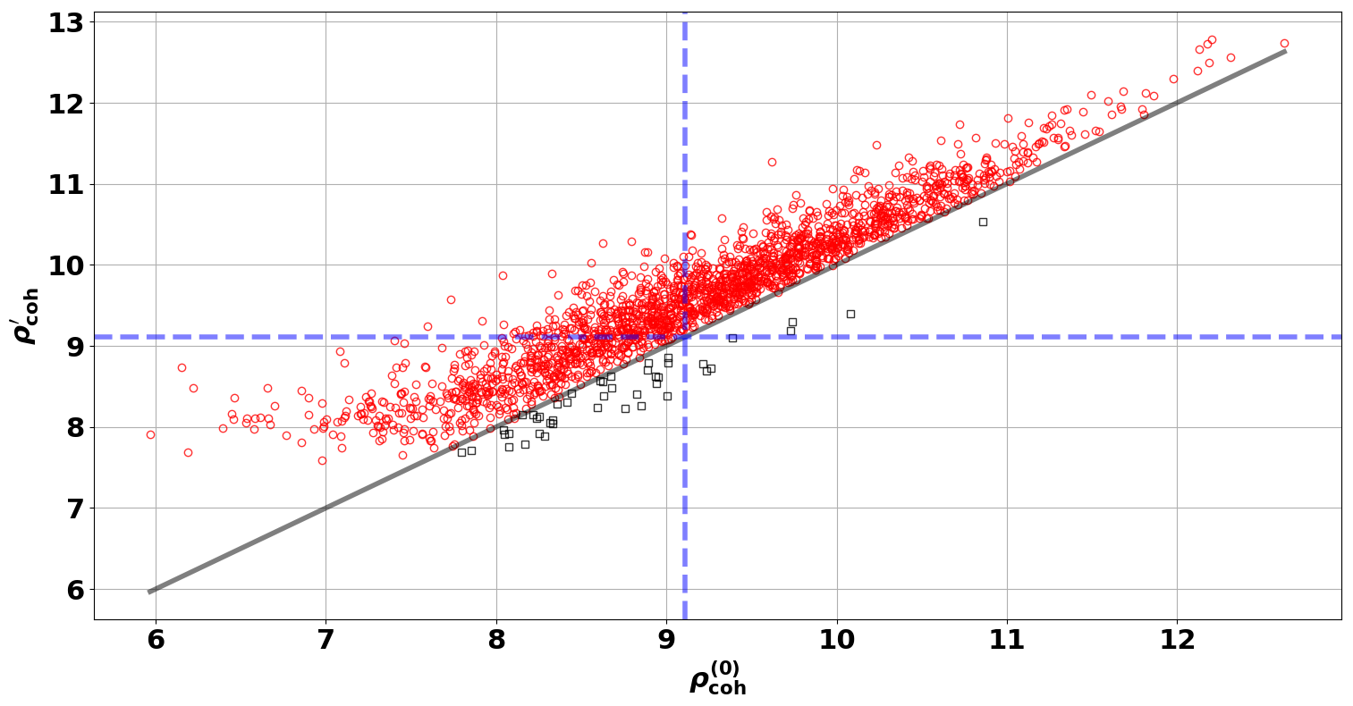
Figure 1: Scatterplot of the best coherent fitness value, $\rho_{\rm coh}^{\prime}(4,1500)$, found by PSO and the coherent fitness at the true signal parameters, $\rho_{\rm coh}^{(0)}$, for ${\rm SNR}_{\rm opt}=9$ and M1 data. Out of a total of 2000 points, 44 (or $2.2\%$) fall below the diagonal. The blue lines show the detection threshold of 9.109.

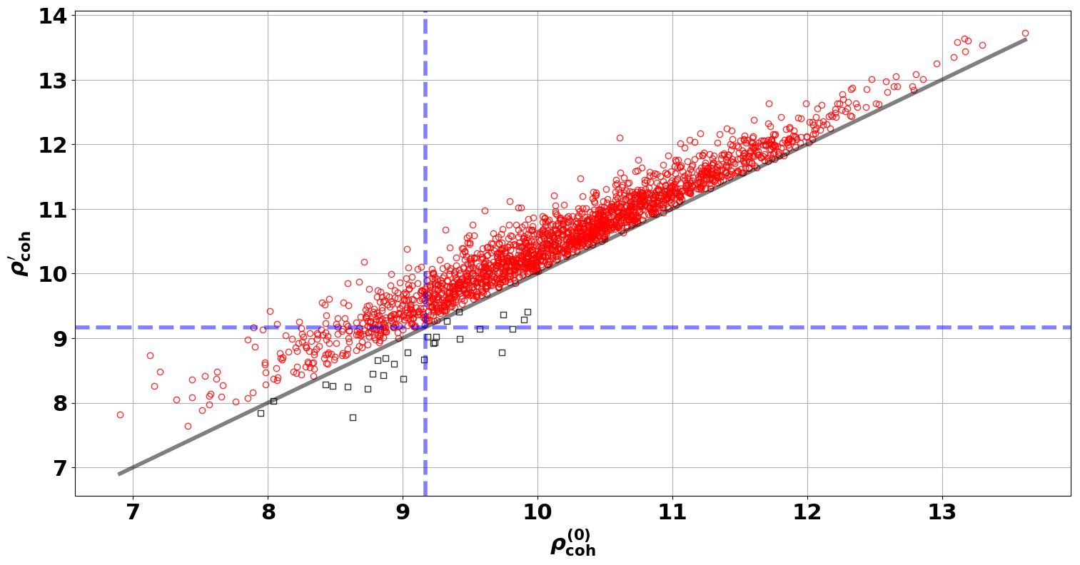
Figure 2: Scatterplot of the best coherent fitness value, $\rho_{\rm coh}^{\prime}(4,1000)$, found by PSO and the coherent fitness at the true signal parameters, $\rho_{\rm coh}^{(0)}$, for ${\rm SNR}_{\rm opt}=10$ and M1 data. Out of a total of 2000 points, 28 (or $1.4\%$) fall below the diagonal. The blue lines show the detection threshold of 9.168.

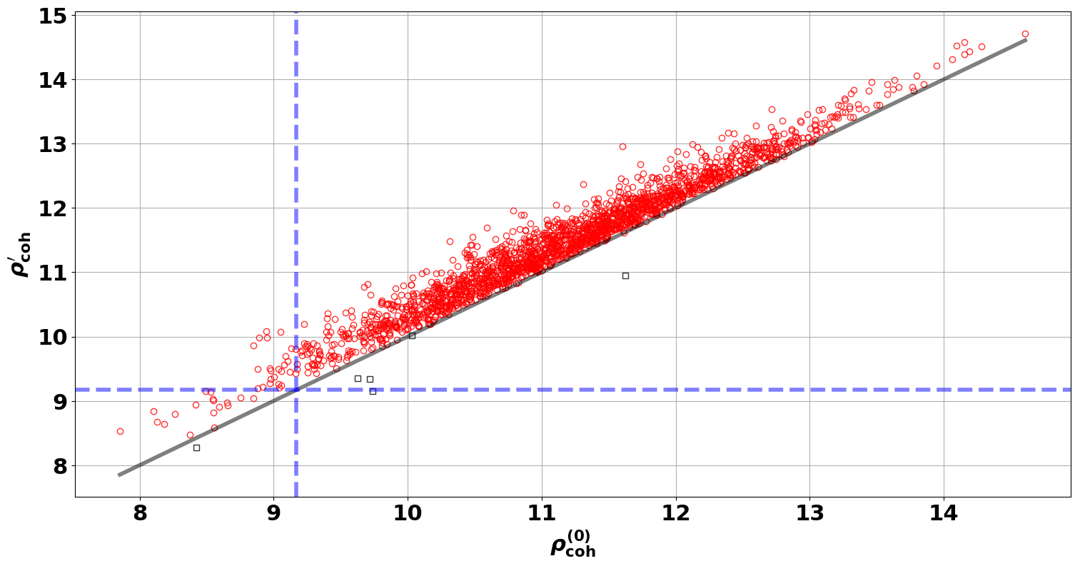
Figure 3: Scatterplot of the best coherent fitness value, $\rho_{\rm coh}^{\prime}(4,1000)$, found by PSO and the coherent fitness at the true signal parameters, $\rho_{\rm coh}^{(0)}$, for ${\rm SNR}_{\rm opt}=11$ and M1 data. Out of a total of 2000 points, 6 (or $0.3\%$) fall below the diagonal. The blue lines show the detection threshold of 9.168.

As expected, the condition $\rho_{\rm coh}^{\prime}\geq\rho_{\rm coh}^{(0)}$ fails in a non-zero fraction of the data realizations. However, the observed performance is a substantial improvement over gbest PSO in WM, where this condition failed in $6.6\%$ of the realizations at ${\rm SNR}_{\rm opt}=12.7$ and $N_{\rm runs}=12$. Here, the same condition fails in $2.2\%$, $1.4\%$, and $0.3\%$ of trials for ${\rm SNR}_{\rm opt}=9$, $10$, and $11$ respectively. Interestingly, the total number of fitness evaluations ($N_{p}\times N_{\rm iter}\times N_{\rm runs}$) per data realization, which was found to be $2.4\times 10^{5}$ for gbest PSO in WM, remains the same for lbest PSO despite the lower ${\rm SNR}_{\rm opt}$ of $9$. The number of fitness evaluations shrinks, compared to gbest PSO, to $1.6\times 10^{5}$ at the higher ${\rm SNR}_{\rm opt}$ values.

Interestingly, out of the $44$, $28$, and $6$ points that fall below the diagonal in Fig. 1 to Fig. 3 respectively, $42$, $28$, and all $6$ arise from data realizations associated with the L5 location. We do not understand the origin of this effect at present. The L5 location also seems to be associated with a prominent secondary maximum, discussed in Sec. IV.3, of the coherent fitness function. It is likely that these effects are linked.

The tuning process described above pertains to the specific length of M1 data. However, the optimum settings for a given data length can serve as useful starting points for other cases. We illustrate this with the challenging case of M2 where the data length is $\approx 30$ times longer than that for M1. Since the current computation time for the M2 data is extremely long ($\approx 18$ hours), carrying out a statistically reliable tuning with a sufficiently large number of data realizations is not feasible. Instead, we simply start with the optimum settings found for a given ${\rm SNR}_{\rm opt}$ in Table 1 and explore variations around those settings. Considering the case of ${\rm SNR}_{\rm opt}=11$ and starting with the tuned settings ($N_{\rm runs}=4$ and $N_{\rm iter}=1000$) for M1 data, we found that the performance of PSO was not acceptable. However, by increasing $N_{\rm iter}$ to 1500 and $N_{\rm runs}$ to $8$ a reasonably effective performance level was achieved.

Fig. 4 shows the scatterplot of $\rho^{\prime}_{\rm coh}$ and $\rho_{\rm coh}^{(0)}$ for data realizations containing the M2 signal with ${\rm SNR}_{\rm opt}=11$. There are $25$ realizations of M2 data for each of the two sky locations (L4 and L5). The fraction of trials in which the condition $\rho^{\prime}_{\rm coh}\geq\rho_{\rm coh}^{(0)}$ fails is now at $8\%$. As observed in the case of M1 data, these dropouts again arise from the data realizations associated with the L5 location. The fraction of failures should go down with an increase in ${\rm SNR}_{\rm opt}$ and further improvements in performance should be possible with some more exploration of $N_{\rm runs}$ and $N_{\rm iter}$.

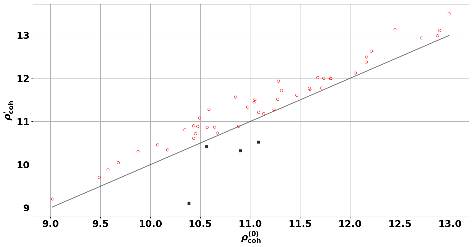
Figure 4: Scatterplot of the best coherent fitness value, $\rho_{\rm coh}^{\prime}(8,1500)$, found by PSO and the coherent fitness at the true signal parameters, $\rho_{\rm coh}^{(0)}$, for ${\rm SNR}_{\rm opt}=11$ and M2 data. Out of a total of 50 points, 4 (or $8\%$) fall below the diagonal.

IV.2 Detection performance

Having obtained the best settings for PSO following the tuning strategy described in Sec. IV.1, we can characterize the detection and estimation performance that can be expected from the PSO-based search. This is done almost exclusively for the M1 signal in this paper because our current computing resource limitations do not allow a reasonably large number of data realizations, especially under $H_{0}$, to be used for the M2 signal. For M1, we use the same data realizations that were used in the validation (c.f., Fig. 1 to Fig. 3) of tuned settings. The number of noise-only data realizations under $H_{0}$ is $1000$ for each of the two $N_{\rm runs}$ and $N_{\rm iter}$ combinations obtained from the tuning process.

Figures 5, 6, and 7 show the distributions of the coherent search statistic found by PSO for the different data sets described above. A two-sample Kolmogorov-Smirnoff (KS) test is performed on the samples associated with the two sky locations. In all cases, the test supports the null hypothesis that the two samples are drawn from the same distribution. This shows that, as happens in the case of a grid-based search, the distribution of the coherent search statistic found by PSO depends only on ${\rm SNR}_{\rm opt}$ and not the details of the individual detector responses that vary with the source location.

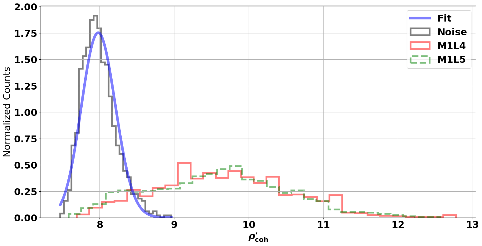
Figure 5: Histograms of the coherent search statistic found by PSO, $\rho^{\prime}_{\rm coh}(4,1500)$, for $H_{0}$ and $H_{1}$ data realizations. The latter contain the M1 signal with ${\rm SNR}_{\rm opt}=9$ at two different sky locations (L4 and L5). The p-value of a two-sample Kolmogorov-Smirnov test between the samples corresponding to L4 and L5 is $0.13$.

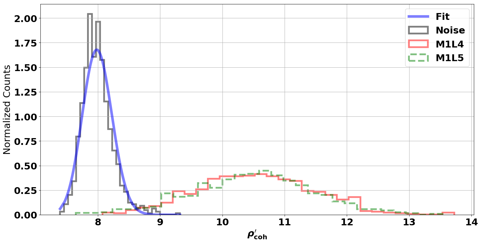
Figure 6: Histograms of the coherent search statistic found by PSO, $\rho^{\prime}_{\rm coh}(4,1000)$, for $H_{0}$ and $H_{1}$ data realizations. The latter contain the M1 signal with ${\rm SNR}_{\rm opt}=10$ at two different sky locations (L4 and L5). The p-value of a two-sample Kolmogorov-Smirnov test between the samples corresponding to L4 and L5 is $0.46$.

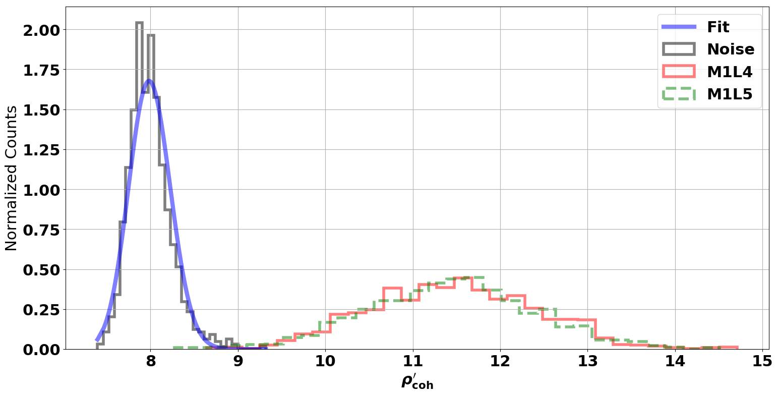
Figure 7: Histograms of the coherent search statistic found by PSO, $\rho^{\prime}_{\rm coh}(4,1000)$, for $H_{0}$ and $H_{1}$ data realizations. The latter contain the M1 signal with ${\rm SNR}_{\rm opt}=11$ at two different sky locations (L4 and L5). The p-value of a two-sample Kolmogorov-Smirnov test between the samples corresponding to L4 and L5 is $0.75$.

We fit a lognormal probability density function (pdf) to the distribution of the coherent search statistic under $H_{0}$ and obtain the detection threshold from this fit for a given false alarm probability (FAP). For a ${\rm FAP}=2.03\times 10^{-6}$, which corresponds to a false alarm rate (FAR) of $1$ event/year, the detection thresholds for the two different PSO settings, $(N_{\rm runs}=4,N_{\rm iter}=1500)$ and $(N_{\rm runs}=4,N_{\rm iter}=1000)$, differ only marginally at $9.109$ and $9.168$ respectively. Table 2 lists the detection probabilities at these thresholds for different ${\rm SNR}_{\rm opt}$ values. We see that the sensitivity of a PSO-based fully-coherent all-sky search reaches an interesting level at around ${\rm SNR}_{\rm opt}\approx 9$.

Table 2: Detection probabilities for the M1 signal at a FAR of 1 false event per year (${\rm FAP}=2.03\times 10^{-6})$. Also listed is the loss in detection probability, $L_{\rm DP}$, defined in Eq. 38.

${\rm SNR}_{\rm opt}$	L4	L5	$L_{\rm DP}$
$9$	0.72	0.692	$0.39\%$
$10$	0.934	0.903	$0.48\%$
$11$	0.995	0.985	$0.05\%$

As discussed in Sec. IV.1, PSO has a finite probability of not converging to the global maximum of the coherent fitness function. This is shown by the points that fall below the diagonal in Fig. 1 to Fig. 4. However, failure to converge to the global maximum does not necessarily mean failure to detect a signal since the coherent search statistic, $\rho_{\rm coh}^{\prime}$, obtained from PSO may still exceed the detection threshold. Detection probability is only reduced when $\rho_{\rm coh}^{\prime}$ falls both below the diagonal and below the detection threshold.

We define the loss in detection probability as

$$L_{\rm DP} = P(\rho^{\prime}_{\rm coh}\leq\eta|\rho^{(0)}_{\rm coh}\geq\eta)\;,$$ (38)

where $P(A|B)$ denotes the conditional probability of event $A$ given event $B$, and $\eta$ is the detection threshold. As seen from Table 2, the estimated $L_{\rm DP}$ is negligible in all cases for the M1 signal at a FAR of 1 false event per year.

As mentioned earlier, we do not have a sufficiently large number of trials under $H_{0}$ for M2 data to reliably estimate the detection threshold for a realistically small FAP. Instead, we simply pick an ad hoc range of $9.0\leq\eta\leq 11.0$ for the detection threshold in this case and find that $L_{\rm DP}$ varies between $2\%$ and $6\%$.

IV.3 Estimation performance

Most analyses Abbott et al. (2018); Veitch et al. (2015) of parameter estimation for the fully-coherent all-sky CBC search report Bayesian credible regions. A credible region ${\rm CR}_{\alpha}$ is the smallest volume in signal parameter space that encloses a fraction $\alpha$ of the total posterior probability. As such, ${\rm CR}_{\alpha}$ is derived from a single data realization. It should be emphasized that ${\rm CR}_{\alpha}$ is in general not equivalent to a Frequentist confidence region in that it is not guaranteed to cover the true parameter values with a probability of $\alpha$ over multiple data realizations. The reduced computational cost of the PSO-based search makes it feasible to obtain Frequentist errors for point parameter estimates using multiple data realizations.

In this paper, we do a limited examination of parameter estimation errors by focusing on only the M1 signal at ${\rm SNR}_{\rm opt}=11$ for which its detection probability is nearly unity. A more thorough examination of this topic will be the subject of future work.

Fig. 8 shows the estimated locations on the sky for both L4 and L5. As was observed in WM for the case of initial LIGO PSD, the error in sky location generally follows its dependence on the condition number of the antenna pattern matrix: the estimated locations are distributed over a much more extended region when the source location has a higher condition number.

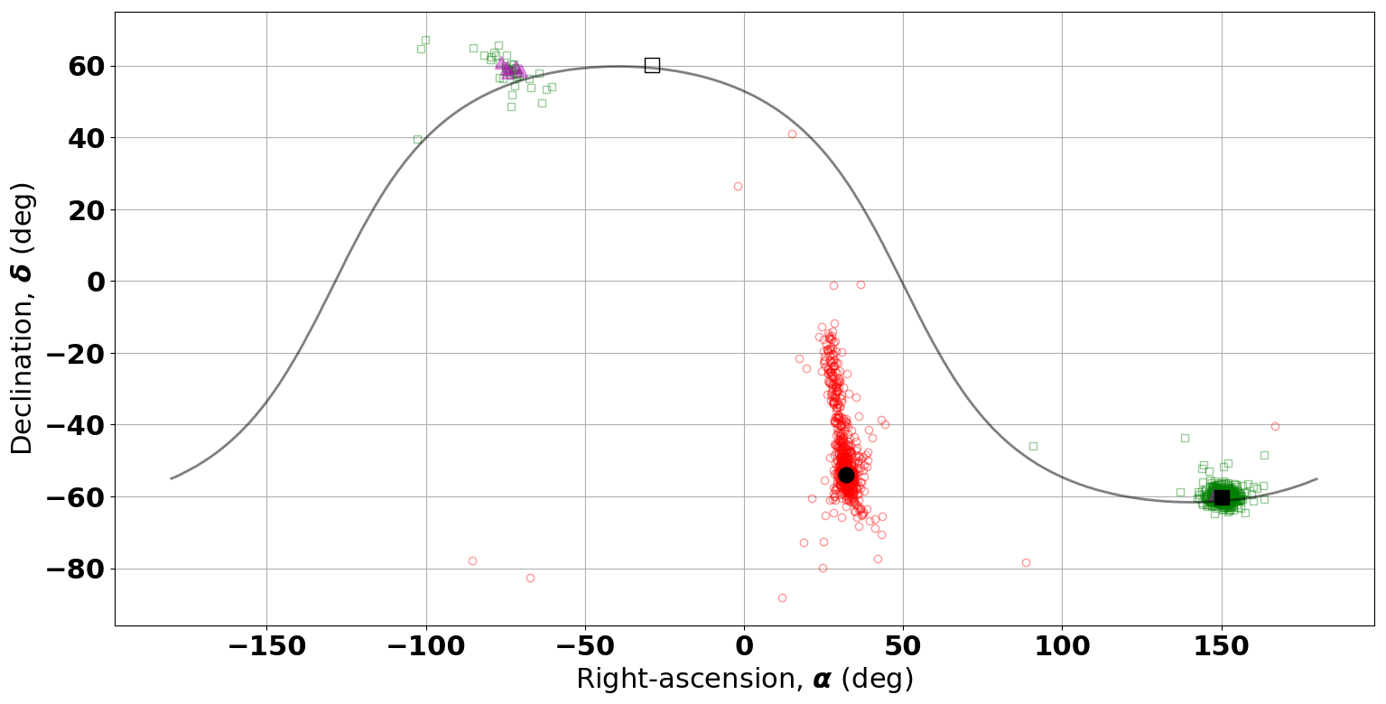
Figure 8: Estimated sky locations for a ${\rm SNR}_{\rm opt}=11$ M1 signal at the L4 (red) and L5 (green and magenta) sky locations. The true sky locations for L4 and L5 are denoted by the filled black circle and square respectively. All $6$ of the data realizations for which the condition $\rho_{\rm coh}^{\prime}\geq\rho_{\rm coh}^{(0)}$ failed, indicating failure in finding the global maximum of the coherent fitness function, are associated with the L5 location and are marked by magenta triangles. The secondary maximum associated with L5 lies along the great circle (solid curve) joining L5 with its antipodal point (empty black square).

A caveat to the empirical rule of thumb above is that the L5 location, while exhibiting a more compact distribution of the estimates, also shows a widely separated secondary maximum. Going by the condition $\rho^{\prime}_{\rm coh}\geq\rho^{(0)}_{\rm coh}$ as an indicator of convergence to the global maximum, we find that the global maximum shifted to the secondary in $4.3\%$ of the trials where this condition was met. At the same time, all but one of the trials where this condition failed also appear at the secondary maximum. Thus, PSO does not go to an arbitrary location but latches on to the secondary when it fails to locate the global maximum. These observations indicate that the secondary maximum is a genuine feature of the coherent fitness function when a source is located at L5 and not an artifact of using PSO.

Fig. 9 shows the estimation error distribution for chirp times $\tau_{0}$ and $\tau_{1.5}$. The main observation here is that these errors are essentially uncorrelated with the errors in sky localization. This is expected from a Fisher information analysis but, as was pointed out in WM, this need not be true for some sky locations.

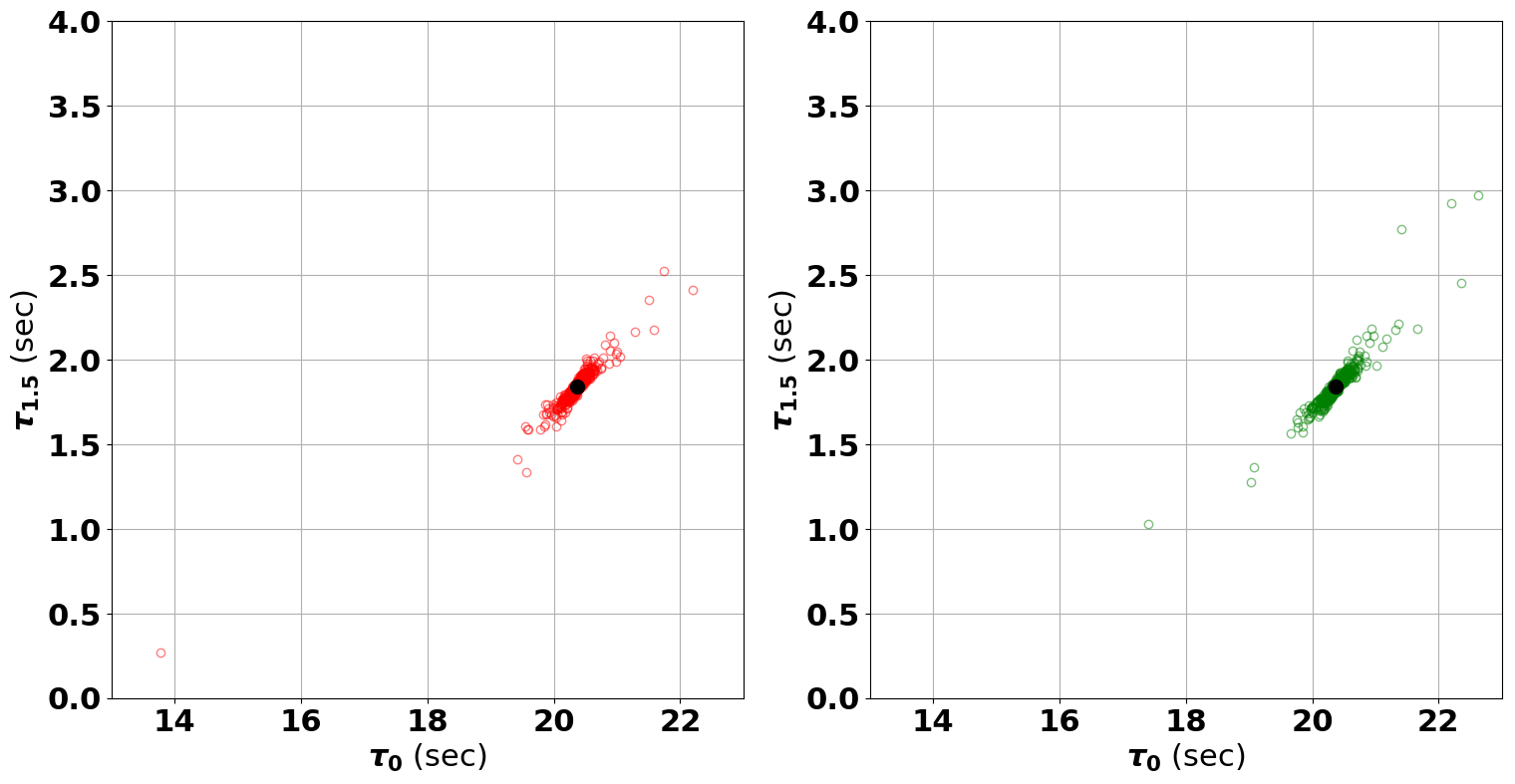
Figure 9: Shown are the estimated chirp times for 1000 realizations of a $\rho_{\rm coh}^{(0)}=11$ signal at the M1L4 and M1L5 sky locations using $\rho_{\rm coh}^{\prime}(4,1000)$. The true chirp time is marked by a black circle for L4 and L5, respectively.

V Computation time analysis

As demonstrated by the rich science payoffs from the joint GW and EM observations of GW170817, the detection of EM counterparts of CBC events is of critical importance. A key factor here is the time elapsed in the dissemination of a follow up alert to EM astronomers.

While the time needed to generate an alert depends on a number of factors, including manual vetting of detector state and data quality, the execution time of the GW search algorithm is the primary determinant. With this in mind, it is important to analyze the computation time of a PSO-based fully coherent search.

The results in this paper are obtained using a code that is implemented in the C programming language. There are two nested layers of parallelization in the code. In the outer layer, parallelization is performed over the independent PSO runs, while the inner layer parallelizes over the PSO particles.

The outer parallelization does not involve any communication between the parallel processes. It is implemented using a framework for high throughput computing called launcher A Wilson et al. (2017) that allows running large collections of independent applications on batch-scheduled clusters. The inner parallelization is implemented as a multi-threaded application based on OpenMP Dagum and Menon (1998); OpenMP Architecture Review Board (2008), which assigns the fitness calculation for each particle to a unique thread that acts as an effectively independent processing unit.

On the cluster used for obtaining the results in this paper (TACC Lonestar 5 Center (2018)), each independent PSO run is assigned to a separate node, with each node providing up to 48 independent threads (24 processing cores with 2 hardware threads per core). On a given node we assign one thread to each particle, which allows for a parallel calculation of the $N_{p}=40$ particle fitness values computed in each iteration of PSO.

Our current parallelization strategy results in the time taken by the whole code running across all the nodes and threads of the cluster being essentially equivalent to the wall-clock computation time, $T_{\rm comp}$, for one thread. Fig. 10 shows $T_{\rm comp}$ as a function of the duration, $T_{\rm data}$, of the data segment analyzed.

We obtain the $T_{\rm comp}$ values shown by averaging over $4$ PSO runs with $N_{\rm iter}=1000$ in each run. A linear fit to the data shows that $T_{\rm comp}$ increases at the rate of $37.2$ min per min of data.

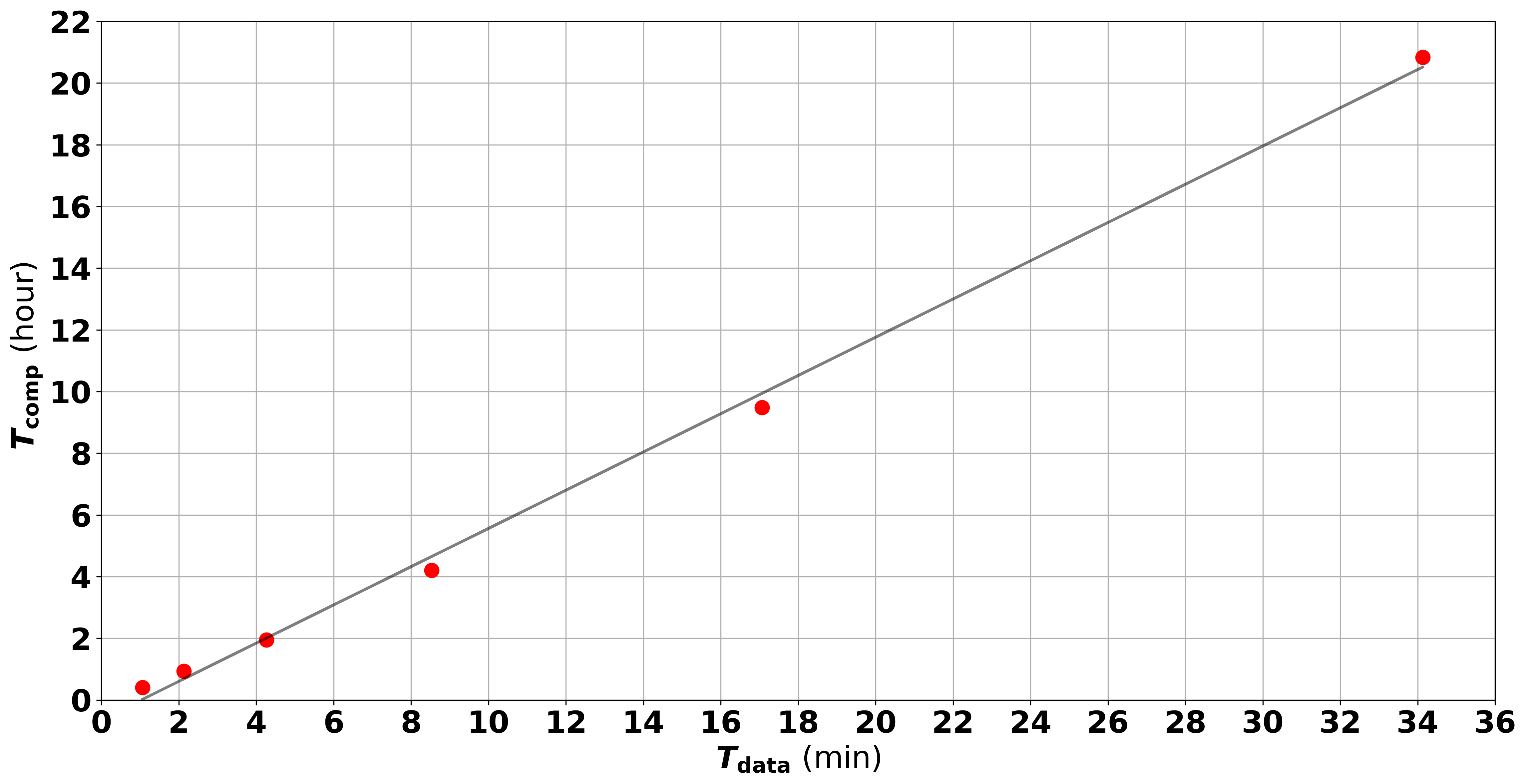
Figure 10: Shown is the computation time, $T_{\rm comp}$, versus data length, $T_{\rm data}$, for $N_{\rm iter}=1000$. A linear fit gives $37.2$ min of computation time per minute of data. The scatter in the computation time across the different PSO runs is in the range of seconds for all the data lengths above and negligible compared to the average.

In the current implementation, all operations involved in a single fitness evaluation are serialized. However, the principal steps in a single fitness evaluation are themselves highly parallelizable. Each fitness evaluation involves (i) generating the $h_{+,\times}$ waveforms, and (ii) computing the inner product in Eq. 17.

Generating the $h_{+,\times}$ waveforms involves independent calculations of the stationary phase approximant of the 2PN waveform Blanchet et al. (1995) at each of the Fourier frequencies in the data. In addition, the inner product in Eq. 17 involves computing the integrand at each Fourier frequency independently.

Thus, an alternative parallelization scheme in a single PSO run is to invert the current scheme by evaluating the fitness values of the $N_{p}$ particles serially and parallelizing over the array operations involved in each fitness evaluation. If the computation time for a single fitness evaluation is $T_{\rm ff}$, the current $T_{\rm comp}$ is approximately $N_{\rm iter}T_{\rm ff}$. With the alternative scheme $T_{\rm comp}\approx N_{p}N_{\rm iter}(T_{\rm ff}/N_{\rm threads})$, where $N_{\rm threads}$ is the number of threads used in parallelizing the fitness function evaluation. Thus, $N_{\rm threads}$ must be substantially greater than $N_{p}$ in order to make the switch to the alternative scheme beneficial.

With high performance computing moving increasingly towards massive hardware-level parallelism, such as the Intel Xeon Phi Knights Landing (KNL) processor with $272$ threads or Graphics Processing Units (GPUs) such as the Nvidia V100 with $5120$ threads, we are already in the regime where $N_{\rm threads}\gg N_{p}$. Thus, the alternative scheme described above could lead to a substantially faster implementation of the fully-coherent all-sky search.

At present, the only objective metric for comparison of computational costs between the PSO-based search and the fully-coherent all-sky search pipeline, LALInference Veitch et al. (2015), used for the analysis of LIGO-Virgo data is the total number of fitness (i.e., likelihood) evaluations. The number of fitness evaluations reported in Veitch et al. (2015) range between $10^{6}$ and $10^{8}$ for the Markov Chain Monte Carlo (MCMC) algorithm using a network of first generation detectors and a data segment length of $32$ sec. The PSO-based search for second generation detectors continues to maintain the same number of fitness evaluations as found in WM for a first generation network, ranging from a maximum of $2.4\times 10^{5}$ to $4.8\times 10^{5}$ for the $64$ sec and $30$ min long data segments respectively. The number of fitness evaluations per independent run of PSO is a factor of $4$ and $8$ smaller for the respective data lengths.

While the PSO-based search incurs a drastically smaller number of fitness evaluations to compute the coherent search statistic and point estimate of the signal parameters, it should be emphasized that MCMC also provides information about the shape of the posterior probability density function. It may be possible to use the PSO-based search results as a seed to focus the MCMC sampling to a smaller region of parameter space and reduce the computational cost of the latter.

It is also worth noting here that, compared to an MCMC search, the PSO-based search involves very few tunable parameters, namely, only $N_{\rm runs}$ and $N_{\rm iter}$.

VI Conclusion

A fully-coherent all-sky search for CBC signals is implemented that uses PSO as the global optimizer of the joint likelihood function of data from a network of second generation detectors. The results presented here show that PSO allows a significant reduction in the computational cost of this search with negligible loss in sensitivity.

At a FAR of 1 event/year, the PSO-based search achieves a detection probability of $\approx 0.7$ at ${\rm SNR}_{\rm opt}=9.0$ for a $20.8$ sec long signal, corresponding to an equal mass binary with $14.5$ $M_{\odot}$ components. For the same signal, the detection probability is $\approx 0.99$ at ${\rm SNR}_{\rm opt}=11$. These results demonstrate that the reduced computational cost is achieved without any significant loss of sensitivity in an astrophysically relevant range of signal strength and binary masses.

Low mass binaries ($O(1.4)$ $M_{\odot}$ components) pose an extreme challenge to fully-coherent all-sky searches with second generation detectors because the signal length becomes $O(30)$ min. We tested the PSO-based search on a $23$ min signal, corresponding to an equal mass binary with $1.506$ $M_{\odot}$, embedded in $30$ min long data segments. We find that the PSO-based search continues to perform well with $\leq 6\%$ loss in detection probability at ${\rm SNR}_{\rm opt}=11$ for a realistic detection threshold of $\approx 10$ on the coherent search statistic.

Going beyond Fisher information analyses and Bayesian credible regions obtained with single data realizations, the reduced computational cost afforded by PSO allows Frequentist parameter estimation errors using multiple data realizations to be obtained. A limited study in this paper shows several interesting issues such as (i) variations in localization errors caused by the condition number of the network antenna pattern matrix, (ii) non-Gaussianity in the sky localization estimation error, and (iii) degenerate locations on the sky. A more extensive and realistic parameter estimation study using the PSO-based search will be carried out in the future.

The prospects for further reductions in the computation time of the PSO-based search are very promising. As discussed in the paper, existing and upcoming hardware-level support for massive parallelism could make an alternative parallelization scheme significantly faster than the current one. Incorporating faster waveform generation schemes, such as the one proposed in Vinciguerra et al. (2017), could reduce the computation time even further. It may even be possible to squeeze out a factor of few from the current code with more efficient implementations of the mathematical formalism. We are currently exploring these possibilities and hope to further push the fully-coherent all-sky search towards real time processing of data.

References

- Abbott et al. (2016) B. P. Abbott et al. (LIGO Scientific Collaboration and Virgo Collaboration), Phy. Rev. Lett. 116, 131103 (2016).
- Acernese et al. (2015) F. Acernese et al., Classical and Quantum Gravity 32, 024001 (2015).
- Abbott et al. (2016a) B. P. Abbott et al. (LIGO Scientific Collaboration and Virgo Collaboration), Phys. Rev. Lett. 116, 061102 (2016a).
- Abbott et al. (2016b) B. P. Abbott et al. (LIGO Scientific Collaboration and Virgo Collaboration), Phys. Rev. Lett. 116, 241103 (2016b).
- Abbott et al. (2017a) B. P. Abbott et al. (LIGO Scientific and Virgo Collaboration), Phys. Rev. Lett. 118, 221101 (2017a).
- Abbott et al. (2017b) R. Abbott, , et al. (LIGO Scientific Collaboration and Virgo Collaboration), Phys. Rev. Lett. 119, 141101 (2017b).
- Abbott et al. (2017c) B. P. Abbott et al. (LIGO Scientific Collaboration and Virgo Collaboration), Phys. Rev. Lett. 119, 161101 (2017c).
- Abbott et al. (2017d) B. P. Abbott et al., The Astrophysical Journal Letters 848, L12 (2017d).
- Somiya (2012) K. Somiya, Classical and Quantum Gravity 29, 124007 (2012), arXiv:1111.7185 [gr-qc] .
- Unnikrishnan (2013) C. S. Unnikrishnan, International Journal of Modern Physics D 22, 1341010 (2013).
- Fairhurst (2009) S. Fairhurst, New Journal of Physics 11, 123006 (2009).
- Nissanke et al. (2011) S. Nissanke, J. Sievers, N. Dalal, and D. Holz, The Astrophysical Journal 739, 99 (2011).
- Kay (1993) S. Kay, Fundamentals of Statistical Signal Processing, Volume I: Estimation Theory, 1st ed. (Prentice Hall, 1993).
- Helstrom (1968) C. W. Helstrom, Statistical Theory of Signal Detection (Pergamon, London, 1968).
- Macleod et al. (2016) D. Macleod, I. W. Harry, and S. Fairhurst, Phys. Rev. D 93, 064004 (2016).
- Weerathunga and Mohanty (2017) T. S. Weerathunga and S. D. Mohanty, Phys. Rev. D 95, 124030 (2017), arXiv:1703.01521 [gr-qc] .
- Kennedy and Eberhart (1995) J. Kennedy and R. Eberhart, in Neural Networks, 1995. Proceedings., IEEE International Conference on, Vol. 4 (1995) pp. 1942–1948 vol.4.
- Albert Lazzarini (1996) R. W. Albert Lazzarini, Ligo Project Science Requirements Document, Tech. Rep. LIGO-E950018-02 (Laser Interferometer Gravitational Wave Observatory, 1996).
- (19) “http://www.mathworks.com/,” .
- Alfred Leick (2004) D. T. Alfred Leick, Lev Rapoport, GPS Satellite Surveying (Wiley, 2004).
- Rakhmanov (2006) M. Rakhmanov, Classical and Quantum Gravity 23, 673 (2006), gr-qc/0604005 .
- Wang and Mohanty (2017) Y. Wang and S. D. Mohanty, Phys. Rev. Lett. 118, 151104 (2017).
- Shoemaker (2010) D. Shoemaker, Advanced LIGO anticipated sensitivity curves, Tech. Rep. LIGO Document T0900288-v3 (Laser Interferometer Gravitational Wave Observatory, 2010).
- Blanchet et al. (1995) L. Blanchet, T. Damour, B. R. Iyer, C. M. Will, and A. G. Wiseman, Phys. Rev. Lett. 74, 3515 (1995).
- Helstrom (1995) Helstrom, Elements of Signal Detection and Estimation (Prentice Hall, 1995).
- Bose et al. (2011) S. Bose, T. Dayanga, S. Ghosh, and D. Talukder, Classical and Quantum Gravity 28, 134009 (2011).
- Sathyaprakash and Dhurandhar (1991) B. S. Sathyaprakash and S. V. Dhurandhar, Phys. Rev. D 44, 3819 (1991).
- Bratton and Kennedy (2007) D. Bratton and J. Kennedy, in Swarm Intelligence Symposium, 2007. SIS 2007. IEEE (IEEE, 2007) pp. 120–127.
- Wang and Mohanty (2010) Y. Wang and S. D. Mohanty, Phys. Rev. D 81, 063002 (2010).
- Bradley Efron (1998) R. J. T. Bradley Efron, An introduction to the bootstrap (Chapman & Hall/CRC, 1998).
- Abbott et al. (2018) B. P. Abbott et al., Living Reviews in Relativity 21, 3 (2018).
- Veitch et al. (2015) J. Veitch et al., Physical Review D 91, 042003 (2015).
- A Wilson et al. (2017) L. A Wilson, J. M Fonner, J. Allison, O. Esteban, H. Kenya, and M. Lerner, The Journal of Open Source Software 2, 289 (2017).
- Dagum and Menon (1998) L. Dagum and R. Menon, IEEE Comput. Sci. Eng. 5, 46 (1998).
- OpenMP Architecture Review Board (2008) OpenMP Architecture Review Board, “OpenMP application program interface version 3.0,” (2008).
- Center (2018) T. A. C. Center, “Lonestar 5,” https://www.tacc.utexas.edu/systems/lonestar (2018), [Online; accessed 21-May-2018].
- Vinciguerra et al. (2017) S. Vinciguerra, J. Veitch, and I. Mandel, Classical and Quantum Gravity 34, 115006 (2017).