Observing small-scale $\gamma$-ray anisotropies with the Cherenkov Telescope Array

Abstract

Disentangling the composition of the diffuse $\gamma$-ray background (DGRB) is a major challenge in $\gamma$-ray astronomy. It is presumed that at the highest energies, the DGRB is dominated by relatively few, still unresolved point sources. This conjecture has recently been supported by the measurement of small-scale anisotropies in the DGRB by the Fermi Large Area Telescope (LAT) up to energies of $500\,\mathrm{GeV}$. We show how such anisotropies can be searched for with the forthcoming Earth-bound Cherenkov Telescope Array (CTA) up to the TeV range. We investigate different observation modes to analyse CTA data for small-scale anisotropies and propose the projected extragalactic large-area sky survey as the most promising data set. Relying on an up-to-date model of the performance of the southern CTA, we find that CTA will be able to probe anisotropies in the DGRB from unresolved point sources at a relative amplitude of $C_{\rm P}^{I}/I^{2}_{\rm DGRB}\gtrsim 4\times 10^{-3}\,\mathrm{sr}$ at energies above $30\,\mathrm{GeV}$ and angular scales $\lesssim 1.5{{}^{\circ}}$. Such DGRB anisotropies have not yet been ruled out by the Fermi-LAT. The proposed analysis would primarily clarify the contribution from blazars and misaligned active galactic nuclei to the very-high-energy regime of the DGRB, as well as provide insight into dark matter annihilation in Galactic and extragalactic density structures. Finally, it constitutes a measurement with complementary systematic uncertainties compared to the Fermi-LAT.

1 Introduction

The last decade has marked a major breakthrough in $\gamma$-ray astronomy. The Fermi Large Area Telescope (LAT, [1]), operating since 2008, has resolved thousands of astrophysical $\gamma$-ray sources above energies of 100 MeV [2]. Ground-based instruments like H.E.S.S., MAGIC, and VERITAS revealed over a hundred sources emitting $\gamma$-rays in the very-high-energy (VHE) regime beyond 100 GeV. The presence of diffuse Galactic emission along the Milky-Way plane and its origin in cosmic-ray interaction with the interstellar gas and radiation fields in the Galaxy are well established [4, 5, 6]. The radiation processes giving rise to the diffuse Fermi-bubbles [7] and Loop-I structure [8], extending far above the Galactic disk, are still under debate. Nonetheless, the Fermi-LAT has detected millions of GeV photons, which cannot be attributed neither to resolved localised sources or to known diffuse structures [9, 10]: These $\gamma$-rays compose the so-called diffuse $\gamma$-ray background (DGRB) and, by definition, comprise all $\gamma$-rays outside the Galactic plane with almost isotropic distribution and not assigned to known $\gamma$-ray sources on the sky [11, 12]. Unresolved, far-away extragalactic $\gamma$-ray sources, distributed isotropically on the sky, definitely constitute a major fraction of the DGRB [13, 14, 15, 16, 17, 18]. However, also unresolved sources of Galactic origin at high latitudes [19, 20] and unaccounted large-scale Galactic diffuse emission [12] might contribute to the DGRB. Annihilation of dark matter (DM) particles in the Milky Way halo and throughout the cosmic web might provide an additional, still unidentified $\gamma$-ray source [21, 22, 23]. The relative contributions of numerous Galactic and extragalactic source classes to the DGRB are currently under debate [12].

The prevalence of extragalactic sources in the DGRB is further supported by the recent observation of its spectral softening below $1\,\mathrm{TeV}$ [10], in agreement with an attenuation due to pair-production losses from interaction with the extragalactic background light (EBL, [24]). If the DGRB is of mostly extragalactic origin, it must necessarily become more anisotropic at higher energies. Any known physical process generating $\gamma$-rays can only occur in the surroundings of galaxies or galaxy clusters, which appear virtually point-like on the sky for current $\gamma$-ray telescopes. The $\gamma$-rays arriving from these far-away sources are redshifted by the cosmic expansion and attenuated by the EBL, with the latter effect being stronger the higher the $\gamma$-ray energy [25]. For these reasons, only relatively close or spectrally hard objects are expected to emit $\gamma$-rays that are observable at VHE energies, independent of the specific production mechanism at source. This conjecture is in agreement with the identified extragalactic sources in the third Fermi-LAT full-sky catalogue of hard-spectra $\gamma$-ray sources (3FHL) [26] and the angular directions and redshifts of known VHE $\gamma$-rays emitters.

Focusing on such anisotropic signatures of the DGRB to decipher its origin, the approach of an angular power spectrum (APS) analysis was first applied to data from the Fermi-LAT several years ago. An anisotropic component to the DGRB on angular scales $\lesssim 2^{\circ}$ (“small-scale anisotropies”) was in fact observed [27]. The amplitude of these anisotropies was found compatible with being constant on all investigated angular scales, suggesting that the APS signal is caused by unclustered point sources.

A recent analysis up to $500\,\mathrm{GeV}$ based on more than six years of Fermi-LAT data confirmed this finding and indicates a spectral hardening of the underlying sources with increasing energy [28]. The detected APS is in agreement with the prediction for unresolved blazars [29, 30] and misaligned active galactic nuclei (AGN) [31]. However, it has been suggested that also Galactic sources, in particular high-latitude millisecond pulsars [19], or relic annihilation of Galactic and extragalactic DM [32, 33, 34, 35, 36, 37, 38, 39] might significantly contribute to small-scale DGRB anisotropies.

Further knowledge about the contributors to the DGRB can be obtained by probing its APS in the VHE regime. Due to the large cosmic-ray background, it is highly challenging to measure the absolute intensity of diffuse $\gamma$-rays with Earth-bound $\gamma$-ray detectors. However, the measurement of $\gamma$-ray anisotropies from ground may be much less constrained by the background. It was found by [40] that current instruments and their available data sets provide only limited capabilities for probing VHE anisotropies in the DGRB. However, with the future Cherenkov Telescope Array (CTA, [41]), a relatively large field of view (FOV) of a ground-based instrument will be combined with the best angular resolution ever achieved in $\gamma$-ray astronomy. With CTA, the authors of [40] have shown that a promising sensitivity to small-scale VHE $\gamma$-ray anisotropies can be reached. In the last years, optimization studies for the array layout and detailed studies on the expected performance of CTA have been performed, and dedicated observing plans for the first decade of operation have been drawn [42]. Therefore, this paper presents a refined assessment of CTA’s capability to resolve small-scale anisotropies in the DGRB.

This article is organised as follows: In section 2, we introduce the concept of angular power spectra and describe our likelihood-based analysis method of event data APS. In section 3, we present the instrumental model for the CTA event sampling (§ 3.1) and outline our setup of a CTA extragalactic survey (§ 3.2). We investigate the APS characteristic of the CTA cosmic-ray background and argue to prefer data from a shallow large-area survey for a study of $\gamma$-ray anisotropies (§ 3.3). Section 4 then presents our analysis and results on the CTA sensitivity to small-scale anisotropies. Our findings are finally discussed in section 5 with respect to existing data and expected DGRB anisotropies caused by different source classes. We conclude in section 6.

2 Likelihood-based analysis of event data angular power spectra (APS)

We quantify the anisotropies in the DGRB by decomposing the spatial distribution of $\gamma$-ray-like events into its auto-correlation angular power spectrum (APS), $C_{\ell}$. A square-integrable function $I(\vartheta,\varphi)=I(\vec{k})$ on the sphere can be expressed as a linear combination of spherical harmonics $Y_{\ell m}(\vec{k})$,

$$I(\vec{k})=\sum\limits_{\ell=0}^{\infty}\sum\limits_{m=-\ell}^{m=+\ell}a_{\ell m}\,Y_{\ell m}(\vec{k}).$$ (2.1)

where in the following, $I$ describes $\gamma$-ray intensities or the dimensionless maps of binned $\gamma$-ray event numbers. The $C_{\ell}$ are defined as the covariance of the uncorrelated coefficients $a_{\ell m}$,

$$\langle a_{\ell m}a^{*}_{\ell^{\prime}m^{\prime}}\rangle=C_{\ell}\,\delta_{\ell\ell^{\prime}}\,\delta_{mm^{\prime}}\quad\Rightarrow\quad C_{\ell}=\langle|a_{\ell m}|^{2}\rangle\,.$$ (2.2)

For a statistically isotropic field with $\langle a_{\ell m}\rangle=0$, the ensemble average of the $a_{\ell m}$,

$$\widehat{C}_{\ell}=\frac{1}{2\ell+1}\sum\limits_{m}|a_{\ell m}|^{2}\,,$$ (2.3)

provides an unbiased estimator for $C_{\ell}$. With the common normalisation $\int|Y_{\ell m}(\vec{k})|^{2}\,\mathrm{d}\Omega=1$ it is $[C_{\ell}]=[I]^{2}\times\mathrm{sr}$, and we will denote this dimensional intensity APS in the following with a superscript, $C_{\ell}^{I}$. Throughout this paper, we assume the residual cosmic-ray background for Earth-bound $\gamma$-ray observation to be isotropic with no intrinsic power ($C_{\ell,\,\rm bck}^{I}=0$). However, the shot noise from $N_{\rm ev}$ disjoint total events, binned in $N_{\rm pix}$ pixels, adds a noise power $C_{\rm N}^{I}$ (indicated by the subscript N for noise) to the measurement,

$$C_{\rm N}^{I}=\frac{4\pi\,\mathrm{sr}}{f_{\rm sky}}\;\frac{N_{\rm ev}{}}{N_{\rm pix}{}^{2}}\,,$$ (2.4)

where $f_{\rm sky}=\frac{1}{4\pi\,\rm sr}\,\int W(\vec{k})\,\mathrm{d}\Omega$ is the unmasked part of the sky. With this, we reconstruct the full-sky equivalent signal APS, $C_{\ell,\,\rm sig,\,\rm data}^{I}$, from a measured APS, $C_{\ell,\,\rm raw}^{I}$, to

$$C_{\ell,\,\rm sig,\,\rm data}^{I}=\left(C_{\ell,\,\rm full\mbox{-}sky}^{I}-C_{\rm N}^{I}\right)\times(W_{\ell}^{\rm beam})^{-2}\,,$$ (2.5)

where the power is unfolded by the beam suppression of a radially symmetric point spread function (PSF) $\mathrm{d}P/\mathrm{d}\theta$ [43],

$$W_{\ell}^{\rm beam}(E)=\frac{2\pi\,\rm sr}{\Omega_{B}}\int\limits_{-1}^{1}\;\mathcal{P}_{\ell}(\cos(\theta))\times\frac{\mathrm{d}P}{\mathrm{d}\theta}(\theta,\,E)\;\mathrm{d}(\cos\theta)\,,$$ (2.6)

and $\mathcal{P}_{\ell}$ are the Legendre polynomials of the $\ell$-th order, and $\Omega_{B}=\int\mathrm{d}P/\mathrm{d}\theta\,\mathrm{d}\Omega$. Finally, we make use of the approximation

$$C_{\ell,\,\rm full\mbox{-}sky}^{I}\approx\frac{C_{\ell,\,\rm raw}^{I}}{f_{\rm sky}}$$ (2.7)

to account for the sampling of the APS on a limited sky patch. More precisely, a masking of $I$ with a window $W(\vec{k})$ in angular space results in a convolution in $\ell$-space [44, 45, 46],

$$C_{\ell,\,\rm raw}^{I}=\frac{1}{2\ell+1}\sum\limits_{\ell^{\prime}}\sum\limits_{mm^{\prime}}\,M_{\ell\ell^{\prime}mm^{\prime}}\,C_{\ell^{\prime},\,\rm full\mbox{-}sky}^{I}\,,$$ (2.8)

with the convolution kernel $M_{\ell\ell^{\prime}}$,

$$M_{\ell\ell^{\prime}mm^{\prime}}=\int_{\Omega}\,W(\vec{k})\,Y^{*}_{\ell m}(\vec{k})\,Y_{\ell^{\prime}m^{\prime}}(\vec{k})\,\mathrm{d}\Omega\,.$$ (2.9)

At sufficiently large $\ell$, it is $M_{\ell\ell^{\prime}mm^{\prime}}^{-1}\approx\frac{2\ell+1}{f_{\rm sky}}\;\delta_{\ell\ell^{\prime}}\delta_{mm^{\prime}}$ and Eq. 2.7 holds [45]. However, like in Euclidean Fourier transformation, sharp window edges in angular space cause global spectral leakage artefacts in $\ell$-space. In § 3.3, we will discuss these effects and the amount of spectral leakage for various CTA field of view shapes.

Due to its large residual background, CTA is unable to determine the absolute level of the DGRB intensity, $I_{\rm DGRB}$, which we are ultimately interested in probing for anisotropies. Therefore, we will work with the dimensionless fluctuation APS, $C_{\ell}^{F}:=C_{\ell}^{I}/I^{2}$. For event maps, the fluctuation APS is connected to the intensity APS via

$$C_{\ell,\,\rm sig}^{F}=f_{\rm sky}^{2}\times\left(\frac{N_{\rm pix}}{N_{\rm ev}}\right)^{2}\times C_{\ell,\,\rm sig}^{I}\,.$$ (2.10)

Under the assumption that $I$ consists of two components, $N_{\rm ev}=N_{\rm bck}+N_{\rm DGRB}$, where the background events $N_{\rm bck}$ contain zero intrinsic small-scale anisotropy (despite the shot noise power), the fluctuation APS of the DGRB component can be estimated as

$$C_{\ell,\,\rm DGRB}^{F}=C_{\ell,\,\rm sig}^{F}\times\left(\frac{N_{\rm ev}}{N_{\rm DGRB}}\right)^{2}\,.$$ (2.11)

Note that the estimated number $N_{\rm DGRB}$ of $\gamma$-ray events in the data set must be calculated with some a priori knowledge, e.g, using a spectrum measured by the Fermi-LAT and the expected CTA instrumental response. This is what we will later do to interpret the sensitivity towards anisotropies in CTA data in the context of the DGRB.

We finally use a maximum likelihood (ML) approach to estimate the significance of an APS detection and to fit the signal parameters. We tailor our analysis to the assumption that the DGRB is dominated by unresolved point sources, which show an APS constant in multipole [47]. This constant power is indicated by the subscript P for Poisson power:

$$C_{\ell,\,\rm sig,\,model}=C_{\rm P}\,.$$ (2.12)

We pursue an analysis binned in multipoles $\ell$. A binned analysis turns out be necessary to suppress remaining masking artefacts in the range of analysis, i.e., a correlation between neighbouring multipoles. We follow the findings by [28] and use the unweighted arithmetic mean in each bin, $\left\langle{C_{\rm sig,\,data}}\right\rangle_{i}=\sum_{\ell_{\rm min,\,i}}^{\ell_{\rm max,\,i}}\;C_{\ell,\,\rm sig,\,data}/\Delta\ell_{i}$ with $\Delta\ell_{i}=\ell_{\rm max,\,i}-\ell_{\rm min,\,i}+1$. For an isotropic field, Eq. 2.2, the probability density of $C_{\ell}$ follows a $\chi^{2}_{2\ell+1}$ distribution and the error on the binned $\left\langle{C_{\rm sig,\,data}}\right\rangle_{i}$ is [43]

$$\left\langle\sigma_{\ell,\,\rm model}^{\;2}\right\rangle_{i}=\frac{2}{\,f_{\rm sky}\,(\Delta\ell_{i})^{2}}\,\sum_{\ell_{\rm min,\,i}}^{\ell_{\rm max,\,i}}\;\frac{\left(C_{\rm P}^{I}+C_{\rm N}^{I}\times(W_{\ell}^{\rm beam})^{-2}\right)^{2}}{2\ell+1}\,,$$ (2.13)

where we assume $\langle\sigma_{\ell,\,\rm data}^{\;2}\rangle_{i}\approx\langle\sigma_{\ell,\,\rm model}^{\;2}\rangle_{i}\equiv\langle\sigma_{\ell}^{\;2}\rangle_{i}$. We find that a logarithmic binning with $\sim 5$ bins per $\ell-$decade is able to eliminate the multipole correlation due to the masking (which breaks the assumption of Eq. 2.2) and to assure the correct error estimation according to Eq. 2.13.

With these definitions, we construct the likelihood function

$$\mathscr{L}\left(C_{\rm P}^{I}\,|\,\vec{C}_{\rm sig,\,data}^{I}\right)=\prod\limits_{i}^{N_{\rm bins}}\frac{1}{\sqrt{2\pi\,\langle\sigma_{\ell}^{\;2}\rangle_{i}}}\,\exp\left(-\frac{\left[\left\langle C_{\rm sig,\,data}^{I}\right\rangle_{i}-C_{\rm P}^{I}\;\right]^{2}}{2\,\langle\sigma_{\ell}^{\;2}\rangle_{i}}\right)$$ (2.14)

where $\vec{C}_{\rm sig,\,data}^{I}$ denotes the ensemble of reconstructed measured multipoles $C_{\ell,\,\rm sig,\,data}^{I}$.

We then maximise the logarithm of the likelihood $\mathscr{L}$, Eq. 2.14, under the constraint $C^{I}_{\rm P}\equiv 0$ and with $C^{I}_{\rm P}$ allowed to vary, and use the ratio of these maximised log-likelihoods as test statistic,

$$\mathrm{TS} =-2\,\log\left(\frac{\mathscr{L}\left(C_{\rm P}^{I}\equiv 0\,|\,\vec{C}_{\rm sig,\,data}\right)}{\mathscr{L}\left(\widehat{C}_{\rm P}^{I}\,|\,\vec{C}_{\rm sig,\,data}\right)}\right)$$

$$=\sum\limits_{i}^{N_{\rm bins}}\left(\frac{\left[\left\langle C_{\rm sig,\,data}^{I}\right\rangle_{i}-\widehat{C}_{\rm P}^{I}\;\right]^{2}}{\left\langle\widehat{\sigma}_{\ell}^{\;2}\right\rangle_{i}}-\frac{\left\langle C_{\rm sig,\,data}^{I}\right\rangle_{i}^{\;2}}{\left\langle\widehat{\widehat{\sigma}}_{\ell}^{\;2}\right\rangle_{i}}+\log\frac{\left\langle\widehat{\sigma}_{\ell}^{\;2}\right\rangle_{i}}{\left\langle\widehat{\widehat{\sigma}}_{\ell}^{\;2}\right\rangle_{i}}\right)\,,$$ (2.15)

to quantify the significance of some signal $C_{\rm P}^{I}\neq 0$ being present in the data. Here, $\widehat{C}_{\rm P}^{I}$ and $\langle\widehat{\sigma}_{\ell}^{\;2}\rangle_{i}$ are the ML estimators for the signal APS amplitude $C_{\rm P}^{I}$ and its variance according to Eq. 2.13; $\widehat{\widehat{\sigma}}_{\ell}^{\;2}$ denotes the estimated variance under the constraint $C^{I}_{\rm P}\equiv 0$ of no signal present in the data.

3 CTA instrumental characteristic and large-area survey model

3.1 Instrumental performance of the southern CTA

The Cherenkov Telescope Array (CTA) will be the next-generation Imaging Atmospheric Cherenkov Telescope (IACT) array, consisting of two separate arrays to be erected at the Paranal site (Chile) in the southern hemisphere and on La Palma (Spain) in the northern hemisphere. In this paper, we base the performance of CTA on the recently published prod3b-v1 instrumental performance simulation and solely on the southern array, comprising 4 Large-Size Telescopes (LSTs), 25 Mid-Size Telescopes (MSTs), and 70 Small-Size Telescopes (SSTs). We rely on the southern CTA for the sake of simplicity and to consider the presence of SSTs (which are planned to be part only of the southern array), yielding a higher sensitivity in the TeV regime. In contrast to the earlier prod2 characteristics, the prod3b performance estimation provides reliable results for Cherenkov light hitting the camera planes under an incidence angle $\vartheta$ off-axis of the telescopes’ pointing direction, crucial for the study of the CTA survey performance. Note that little has changed with respect to the projected on-axis CTA performance ($\vartheta=0$) between prod2 (as used, e.g., in our previous study [49]) and prod3b.

The instrumental performance characteristics are the result of extensive Monte-Carlo (MC) simulations. These simulations comprise the modelling of all steps in the Cherenkov light emission and detection, from the shower development in the atmosphere to the response of the photosensors in the cameras. Because of the high computational costs, calculations are done in relatively coarse bins of the parameters (elevation and azimuth angle of the pointing, $\gamma$-ray energy, off-axis angle,…) such that we apply suitable analytical descriptions of the various instrument response quantities fitted to their discrete tabulated values. Such a fitting approach instead of interpolation is necessary for this study, where we intend to avoid artefacts in the APS which result from the numerics of the simulation (and would not be present in a CTA data set). We assume that all observations are taken at a zenith angle of $20{{}^{\circ}}$, with equal proportions of southern and northern pointings. Besides the physics in the atmosphere and the instrumental layout, the performance characteristics depend on the chosen analysis cuts. If not explicitly stated differently, all event simulations are based on the CTA performance according to an event selection optimised for $5\,\mathrm{h}$ of observation and without spatial cuts, other than removing events at $\vartheta>6{{}^{\circ}}$ from the camera centre.

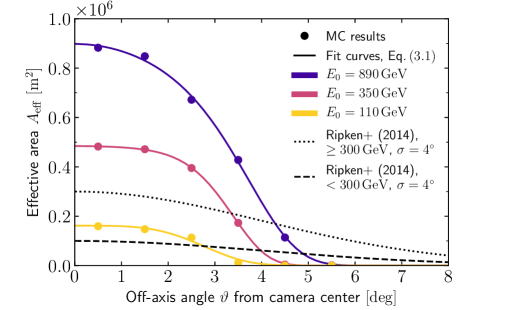
Figure 1: Effective areas for the prod3b southern CTA off-axis performance at different reconstructed $\gamma$-ray energies $\lesssim 1\,\mathrm{TeV}$. The dashed and dotted curves additionally show the earlier CTA effective area models from [40].

We describe the dependence of the effective $\gamma$-ray collection area, $A_{\rm eff}$, and the cosmic-ray residual background rate on the angle $\vartheta$, using a higher-order Gaussian function:

$$f(\vartheta)=A\,\exp\left[-\frac{1}{2}\,\left(\left(\frac{\vartheta}{B}\right)^{6}+\left(\frac{\vartheta}{C}\right)^{4}+\left(\frac{\vartheta}{D}\right)^{2}\right)\right]\,.$$ (3.1)

While previous studies, e.g., [50, 40], have modelled the off-axis behaviour of the CTA effective area and background rate with a Gaussian function ($B=C\equiv\infty$), the modelling by Eq. 3.1 takes into account the plateau shape of the responses around the pointing position. Figure 1 shows the off-axis dependence of $A_{\rm eff}$ for the southern CTA, comparing the MC results for six bins between $\vartheta=0{{}^{\circ}}$ and $\vartheta=6{{}^{\circ}}$ with the fit by Eq. 3.1. This clearly reveals a deviation from a Gaussian shape, in particular at the lowest energies. Figure 1 also displays the Gaussian CTA effective area model in the earlier study on APS measurements with IACTs [40]. Figure 2 shows our off-axis fitting approach for some exemplary prod3b residual background rates (with the abscissa in log-scale, such that a Gaussian scaling would be represented by a parabola). When speaking about the CTA field of view (FOV) in the following, we refer to the energy-dependent off-axis shape of the residual background rate. We define the FOV radius, $\vartheta_{\rm fov}$, via

$$\int_{S^{2}}\frac{\mathrm{d}N_{\rm bck}}{\mathrm{d}\Omega\,\mathrm{d}t}(\vartheta)\,\mathrm{d}\Omega=\frac{\mathrm{d}N_{\rm bck}}{\mathrm{d}\Omega\,\mathrm{d}t}(\vartheta=0)\times\left(1-\cos\vartheta_{\rm fov}\right)\times 2\pi\,\mathrm{sr}\,.$$ (3.2)

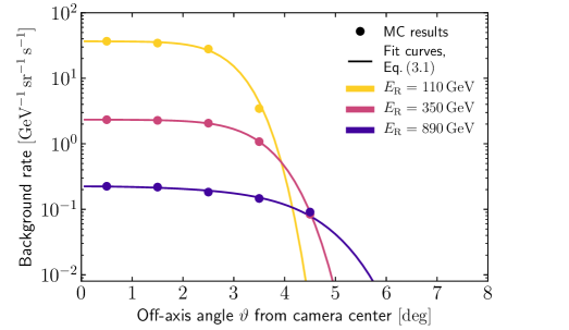
Figure 2: Background rates for the prod3b southern CTA off-axis performance at different reconstructed $\gamma$-ray energies $\lesssim 1\,\mathrm{TeV}$.

In table 1, we show the on- and off-axis event rates above various energy thresholds for the CTA instrumental response used throughout this paper. It can be seen that the FOV radius according to Eq. 3.2 increases with energy, which causes the background over the full FOV to decrease more slowly with energy than the on-axis background rate alone. We also display the expected event rate from a DGRB spectrum after [10], using their foreground model B, which leaves the largest fraction of unassociated $\gamma$-rays to the DGRB:

$$I_{\rm DGRB}=1.12\times 10^{-7}\times\left(\frac{E}{100\,\mathrm{MeV}}\right)^{-2.28}\times\exp\left(-\frac{E}{206\,\mathrm{GeV}}\right)\;\mathrm{cm^{-2}\,s^{-1}\,sr^{-1}\,MeV^{-1}}\,.$$ (3.3)

In table 2, we show the CTA instrumental performance according to the previous work from [40], to be compared with our model in table 1. As shown in figure 1, the authors of [40] assumed a much wider FOV (both for the effective areas and background rates), however, with smaller on-axis effective areas. Combined, they obtain rather similar $\gamma$-ray event rates compared to our prod3b model. Also, their assumption of background rates between $10-100\,\mathrm{Hz}$ above $100\,\mathrm{GeV}$ has remained valid. However, we will argue in § 3.3 that the non-Gaussian and, compared to [40], substantially smaller FOV in the prod3b model provides a major obstacle for analysing deep-field observations for $\gamma$-ray anisotropies.

		DGRB event rate		Background rate		$\gamma$-rays/background
Energy	FOV radius	on-axis	total FOV	on-axis	total FOV	ratio
threshold	$\vartheta_{\rm fov}$	$\mathrm{[Hz\;\deg^{-2}]}$	$\mathrm{[Hz]}$	$\mathrm{[Hz\;\deg^{-2}]}$	$\mathrm{[Hz]}$	on-axis	total FOV
$30\,\mathrm{GeV}$	$2.4{{}^{\circ}}$	$8.8\times 10^{-4}$	$1.6\times 10^{-2}$	3.6	66.2	$2.4\times 10^{-4}$	$2.5\times 10^{-4}$
$100\,\mathrm{GeV}$	$3.3{{}^{\circ}}$	$3.6\times 10^{-4}$	$1.0\times 10^{-2}$	1.1	37.0	$3.3\times 10^{-4}$	$2.7\times 10^{-4}$
$300\,\mathrm{GeV}$	$4.1{{}^{\circ}}$	$4.6\times 10^{-5}$	$1.6\times 10^{-3}$	0.24	12.4	$2.0\times 10^{-4}$	$1.3\times 10^{-4}$
$1\,\mathrm{TeV}$	$5.3{{}^{\circ}}$	$3.2\times 10^{-7}$	$1.3\times 10^{-5}$	0.056	5.0	$5.8\times 10^{-6}$	$2.5\times 10^{-6}$

Table 1: DGRB event rates and background rates (without dead time correction), integrated over energies above different lower thresholds up to $E_{\rm max}=100\,\mathrm{TeV}$. The DGRB rates correspond to the DGRB intensity spectrum according to Eq. 3.3. Events in the “total FOV” comprise all events within the angular direction $\vartheta_{\rm cut}=6{{}^{\circ}}$ from the camera pointing position.

		DGRB event rate		Background rate		$\gamma$-rays/background
Energy	FOV radius	on-axis	total FOV	on-axis	total FOV	ratio
threshold	$\vartheta_{\rm fov}$	$\mathrm{[Hz\;\deg^{-2}]}$	$\mathrm{[Hz]}$	$\mathrm{[Hz\;\deg^{-2}]}$	$\mathrm{[Hz]}$	on-axis	total FOV
$100\,\mathrm{GeV}$	$5.7{{}^{\circ}}$	$1.6\times 10^{-4}$	$1.6\times 10^{-2}$	0.99	100	$1.6\times 10^{-4}$	$1.6\times 10^{-4}$
$300\,\mathrm{GeV}$	$5.7{{}^{\circ}}$	$2.6\times 10^{-5}$	$2.6\times 10^{-3}$	0.099	10	$2.6\times 10^{-4}$	$2.6\times 10^{-4}$

Table 2: Model of the CTA performance from [40], according to their tables 1 & 2, $\sigma_{\rm fov}=4{{}^{\circ}}$, and the assumption of 100/10 Hz background rates above 100/300 GeV. Again, the DGRB rates are computed for the model B from [10]. Note that for a Gaussian off-axis acceptance, $\vartheta_{\rm fov}\approx\sqrt{2}\,\sigma_{\rm fov}$.

The finite CTA angular resolution causes a suppression of the APS at angular scales below the resolution, expressed by Eq. 2.6. The CTA PSF worsens at lower $\gamma$-ray energies $E$ and for large angles $\vartheta$ of the incident $\gamma$-ray in the camera field, i.e. it is $\mathrm{d}P/\mathrm{d}\theta=\mathrm{d}P/\mathrm{d}\theta(\theta;\,E,\,\vartheta)$. We model $\mathrm{d}P/\mathrm{d}\theta(E,\,\theta,\,\vartheta)$ as a two parameter King function [51]

$$\mathrm{d}P/\mathrm{d}\theta(\theta;\,E,\,\,\vartheta)=\frac{1}{2\pi\sigma_{\rm king}}\,\left(1-\frac{1}{\gamma}\right)\,\left(1+\frac{1}{2\gamma}\frac{\theta^{2}}{\sigma_{\rm king}^{2}}\right)^{-\gamma}\,,$$ (3.4)

owing to the fact that CTA will exhibit a PSF with non-Gaussian tails (see the later figure 4). The two parameters $\sigma_{\rm king}=\sigma_{\rm king}(E,\,\,\vartheta)$ and $\gamma=\gamma(E,\,\,\vartheta)$ are again fitted to the MC simulations of the instrumental performance.

3.2 A model of the CTA extragalactic survey

With its large FOV, CTA will be the first IACT array to perform a large-area sky survey [42]. Within the CTA extragalactic survey key science project [42], it is planned to observe $25\%$ of the sky outside the Galactic plane within the first decade of observation. For a total observation time of about $1000\,\mathrm{h}$ with both arrays, such a survey is projected to reach an average sensitivity to fluxes greater than $2.5\times 10^{-12}\,\mathrm{cm^{-2}\,s^{-1}}$ ($0.6\%$ the flux of the Crab Nebula) above $125\,\mathrm{GeV}$ for point sources with a spectrum similar to the one of the Crab Nebula [42]. In this paper, we adopt the same survey field as done in [49] for the extragalactic survey, namely, a circular region around the Galactic south pole, i.e., $b<-30{{}^{\circ}}$. As in [49], we assume that the whole area is covered by the southern array in $500\,\mathrm{h}$, while [42] propose to raster $60\%$ of the survey field in $400\,\mathrm{h}$ with the southern array, and the remaining area in $600\,\mathrm{h}$ with the northern CTA. In this work, we consider a system dead time of 5%, reducing our effective total observation time to $T_{\rm obs}=475\,\mathrm{h}$. Note that this choice is fairly conservative, and CTA is targeted to reach system dead times smaller than $2\%$. On the other hand, we do not consider a loss of observation time due to the telescope slewing between each pointing.

The FOV size of the instrument is critical for the average survey exposure on each spot on the sky and the homogeneity of the exposure. The exposure homogeneity is in particular dependent on the pattern of the pointing distances of the individual survey observations. For the pointing pattern, we adopt a grid relying on the HEALPix pixelisation scheme [52]. The HEALPix tessellation facilitates equally spaced pointing positions on the sphere, where the sphere curvature becomes significant for an area as large as $f_{\rm sky}=0.25$. This large-area survey telescope spacing strategy is illustrated in figure 3. In the remainder of this work, we consider two different grid spacings: A HEALPix grid with ${N_{\rm side}}=32$ results in an average distance between the telescope pointings of $\Delta_{\rm fov}=1.83{{}^{\circ}}\approx 2{{}^{\circ}}$. Hereby, $f_{\rm sky}=0.25$ is covered by 3136 individual pointings with an observation time of $9.6\,\mathrm{min}$ each. This results in an average on-axis equivalent exposure of $t_{\rm obs}\approx 100\,\mathrm{min}$ above $100\,\mathrm{GeV}$ with a homogeneity of $\Delta t/t\lesssim 3\%$. In contrast, a HEALPix grid with ${N_{\rm side}}=64$ is considered, yielding $\Delta_{\rm fov}=0.91{{}^{\circ}}\approx 1{{}^{\circ}}$ with 12,416 single observations over $145\,\mathrm{s}$ each, and the same average exposure $t_{\rm obs}$ above $100\,\mathrm{GeV}$ with $\Delta t/t\lesssim 1\%$.

Because of the lower sensitivity of the northern CTA above 100 GeV compared to the southern array, our simplified large-scale survey setup finally serves as a fairly realistic description of what can be achieved with CTA according to [42]: Using the cssens ctool [51], we find for a dead time corrected on-axis observation with $t_{\rm obs}=95\,\mathrm{min}$ and our selected CTA instrument response a survey sensitivity of $0.4\%$ of the Crab nebula flux above $125\,\mathrm{GeV}$, not more than $30\%$ better than envisaged by [42].

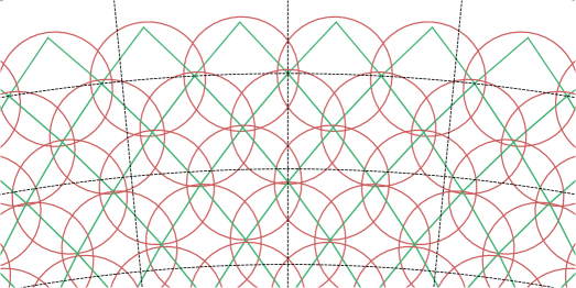
(a) $\Delta_{\rm fov}\approx 4{{}^{\circ}}$ (${N_{\rm side}}=16$)

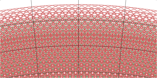
(b) $\Delta_{\rm fov}\approx 1{{}^{\circ}}$ (${N_{\rm side}}=64$)

Figure 3: Large-area survey tiling strategy on $f_{\rm sky}=0.25$ in the HEALPix scheme as adopted in this work. For display purpose only, we show a spacing of $\Delta_{\rm fov}\approx 4{{}^{\circ}}$ (${N_{\rm side}}=16$) in the upper panel. In our default survey setup, we use $\Delta_{\rm fov}\approx 1{{}^{\circ}}$ (lower panel) and compare to $\Delta_{\rm fov}\approx 2{{}^{\circ}}$. The green quadrilaterals show the HEALPix pixels in which the individual telescope pointings are centred. The red circles have a diameter of $6{{}^{\circ}}$ and show the CTA field of view diameter at about $100\,\mathrm{GeV}$. Note that all HEALPix pixels cover the same solid angle, however, they are not congruent.

As the angular resolution degrades with offset from the camera centre, we also have to consider an average angular resolution whose homogeneity is, like the exposure, affected by the observation pattern. We approximate an average PSF under the assumption that each spot on the sky is equally observed under all incidence angles $\vartheta$ from the camera centre up to $\vartheta_{\rm cut}=6{{}^{\circ}}$. In a finite energy interval $[E_{\rm min},\,E_{\rm max}]$, the effective PSF additionally scales with the energy distribution of events from the $\gamma$-ray intensity spectrum $I$. Altogether, we model the effective CTA survey PSF in a finite energy interval as:

$$\left\langle\frac{\mathrm{d}P}{\mathrm{d}\theta}\right\rangle(E,\,\theta)=\frac{\int\limits_{\vartheta_{\rm cut}}\frac{\mathrm{d}P}{\mathrm{d}\theta}(E,\,\theta,\,\vartheta)\times A_{\rm eff}(E,\,\vartheta)\,\mathrm{d}\Omega}{\int\limits_{\vartheta_{\rm cut}}A_{\rm eff}(E,\,\vartheta)\,\mathrm{d}\Omega}\,,\;\left\langle\frac{\mathrm{d}P}{\mathrm{d}\theta}\right\rangle(\theta)=\frac{\int\limits_{E_{\rm min}}^{E_{\rm max}}\left\langle\frac{\mathrm{d}P}{\mathrm{d}\theta}\right\rangle(E,\,\theta)\times I(E)\,\mathrm{d}E}{\int\limits_{E_{\rm min}}^{E_{\rm max}}I(E)\,\mathrm{d}E}.$$ (3.5)

The $\gamma$-ray spectrum $I$ is chosen according to the source class hypothesised in the analysis. Figure 4 shows the averaged PSFs, $\langle{\mathrm{d}P}/{\mathrm{d}\theta}\rangle(E,\,\theta)$, and their corresponding APS attenuation factors $W_{\ell}^{\rm beam}(E)$ at different energies.

The PSF modelling determines the highest multipole $\ell_{\rm max}=1024$ up to which we perform our analysis to avoid the impact of an increasing systematic uncertainty about the PSF at larger $\ell$. This choice of $\ell_{\rm max}$ together with our chosen map resolution also allows us to ignore the power suppression of the data due to the finite bin size (“pixel window”, see right panel of figure 4). Finally, we do not consider the finite energy resolution and energy bias of the CTA instrument in this study. As we investigate the CTA performance in only very coarse energy intervals, the energy resolution of the instrument is negligible.

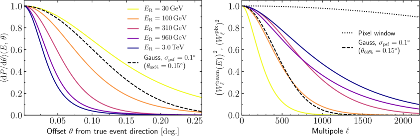
Figure 4: Left panel: Southern CTA angular resolution in terms of the PSF $\langle\mathrm{d}P/\mathrm{d}\theta\rangle(E,\,\theta)$ averaged over $A_{\rm eff}(E,\,\vartheta)$, in angular space at different energies. Right panel: Corresponding window functions in multipole space. A Gaussian curve and its multipole transformation are given for comparison (dashed lines). Also, the pixel window function of a finite HEALPix grid with resolution ${N_{\rm side}}=2048$ is shown (dotted line on the right).

3.3 APS characteristic of the cosmic-ray background in CTA observations

As shown in table 1, CTA suffers from a large irreducible cosmic-ray background. This background constitutes the dominant challenge of power-spectral methods for Earth-bound $\gamma$-ray detectors, in contrast to the similar analyses already performed with Fermi-LAT data.

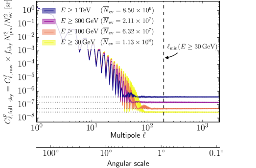
Figure 5: APS of the events from an intrinsically isotropic background in our CTA survey field on $f_{\rm sky}=0.25$ and for an observation spacing of $\Delta_{\rm fov}=1{{}^{\circ}}$. The APS is shown for four different energy thresholds. The dashed vertical line indicates one example of our lower cuts in $\ell$-space. The figure shows the mean $C_{\ell}^{F}$ and the 68% credible intervals (shaded bands) based on 50 simulations each. The grey-dotted lines mark the estimator $C_{\rm N}^{F}=4\pi\,\mathrm{sr}f_{\rm sky}/\overline{N}_{\rm ev}$ for each energy threshold.

To study the APS characteristic of this irreducible background, we use the gammalib and ctools frameworks [51] to simulate hundreds of samples of the background events in our CTA extragalactic survey setup with $\Delta_{\rm fov}=1{{}^{\circ}}$, based on the background rates as presented in § 3.1. Subsequently, we collect the sampled events in maps of $N_{\rm pix}=12\times 2048^{2}$ spatial bins in the HEALPix scheme, and compute the APS of the binned event maps. Figure 5 presents the resulting fluctuation APS above different energy thresholds. The shot noise estimator, Eq. 2.4, is indicated by the dashed horizontal lines in figure 5. It can be clearly seen that the window of the quarter-sky survey field dominates the multipole range at $\ell\lesssim 100$. According to section 2, we assume (i) the approximation $C_{\ell,\,\rm full\mbox{-}sky}^{I}\approx{C_{\ell,\,\rm raw}^{I}}/{f_{\rm sky}}$ to be valid in a regime unaffected by the window above some $\ell_{\rm min}$, (ii) the same for the error described by Eq. 2.13, and (iii) a signal hypothesis with only one additional free parameter in the maximisation of the likelihood Eq. 2.14, namely, $C_{\rm P}\geq 0$. If all these conditions are satisfied, the distribution of TS values from many samples of our background maps must follow a $\chi^{2}$ distribution with one degree of freedom [53],

$$p(\rm{TS})=\frac{1}{2}\,\delta(\rm{TS})+\frac{1}{2}\,\chi^{2}_{k=1}(\rm{TS})\;.$$ (3.6)

Requiring the reproduction of this statistic, we determine

$$\ell_{\rm min}(30\,\mathrm{GeV}\leq E_{\gamma}<100\,\mathrm{GeV}) =200\,,$$

$$\ell_{\rm min}(100\,\mathrm{GeV}\leq E_{\gamma}<300\,\mathrm{GeV}) =150\,,$$

$$\ell_{\rm min}(300\,\mathrm{GeV}\leq E_{\gamma}<1\,\mathrm{TeV}) =120,\,$$

$$\ell_{\rm min}(E_{\gamma}\geq 1\,\mathrm{TeV}) =200$$ (3.7)

as lower limits in $\ell$-space for our analysis. As mentioned in section 2, we find that a binning of the signal and its error in multipoles is crucial to reproduce Eq. 3.6. This procedure worked well for all energy up to $E\leq 1\,\mathrm{TeV}$, whereas at higher energies, window artefacts can no longer be removed by binning for $\ell\lesssim 1000$. For these highest energies, we use $\rm{TS}_{95\%,\,E\geq 1\,\mathrm{TeV}}=8.0$ empirically obtained from our MC simulations, but we emphasise that the results for this bin should be treated with some caution. The cuts $\ell_{\rm min}$ finally define the angular scales $\alpha_{\rm max}\approx 180{{}^{\circ}}/\ell_{\rm min}\leq 1.5{{}^{\circ}}$ below which CTA will be able to probe anisotropies.

Possible deviations of the available data set from the standard survey setup considered in the previous paragraph alter the background APS. Therefore, we have studied (i) the presence of 19 circular exclusion regions with a Gaussian mask and $\sigma=1{{}^{\circ}}$ (corresponding to the 19 up-to-date known VHE $\gamma$-ray sources in the chosen survey field), (ii) a coarser survey grid with $\Delta_{\rm fov}=2{{}^{\circ}}$, and (iii) a 10% variation of the background rate between the individual observation pointings in the survey due to different weather conditions and calibration uncertainty. The latter is a rather conservative estimate, as CTA is required to provide a much more stable data rate over time on all timescales. Figure 6 compares the absolute (left) and relative (right) APS of these varied setups to our standard case from figure 5. The dashed vertical lines in these panels show the $\ell_{\min}$ satisfying the background hypothesis $C_{\ell}=C_{\rm N}$ in our standard survey setup. We conclude that neither the exclusion of some dozens of regions in the survey nor a varying event rate significantly pollute the APS above the threshold $\ell_{\rm min}$ according to Eq. 3.7. However, a coarser survey pattern with $\Delta_{\rm fov}>1{{}^{\circ}}$ in fact adds significant contamination to multipoles above $\ell\geq 120$.

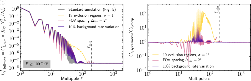
Figure 6: The impact of various deviations from the standard survey simulation onto the residual background APS of events with $E\geq 100\,\mathrm{GeV}$. The relative change of power at each multipole $\ell$ compared to the spectrum presented in figure 5 is shown on the right.

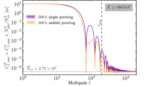
Figure 7: APS of all background events above $100\,\mathrm{GeV}$ in a single CTA pointed observation over $300\,\mathrm{h}$ (for an instrumental response optimised for 50 h of observation). We also show the APS for the $300\,\mathrm{h}$ observation time distributed over four observations, pointed $1.5{{}^{\circ}}$ offset from the central pointing position (“wobble observation mode”). The dotted line shows correspondingly $f_{\rm sky}\times C_{\rm N}^{F}=\frac{4\pi\,\mathrm{sr}}{N_{\rm ev}{}}$. The vertical dashed line denotes the cut applicable for the quarter-sky survey APS (figure 5).

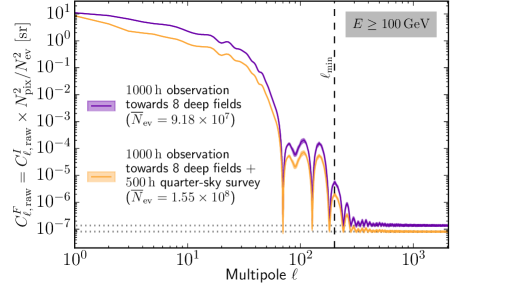
Figure 8: APS of all background events above $100\,\mathrm{GeV}$ towards eight different positions in the sky and a total observation time of $1000\,\mathrm{h}$ (for an instrumental response optimised for 50 h of observation). We also show the APS for these observations combined with the events from a quarter-sky survey.

The authors of [40] also investigated whether a single or some few deep-exposure observations with IACTs can be used for an APS analysis. For their simplified Gaussian model of the CTA field of view (see figure 1), they found a slight increase in sensitivity when investing a fixed total observation time in a single deep field instead of distributing the time over observations of several fields. However, we argue that small field observation data may hardly compete with large-area survey data for a realistic, non-Gaussian CTA instrumental model: Figure 7 shows the APS of the residual background above $100\,\mathrm{GeV}$ in a deep exposure ($300\,\mathrm{h}$) towards a single spot in the sky, where $C_{\ell,\,\rm raw}^{F}=N_{\rm pix}^{2}/N_{\rm ev}^{2}\times C_{\ell,\,\rm raw}^{I}$. The figure reveals dominant lobes in the spectrum which are not present in the multipole transformation of a simple Gaussian function [40]. The dashed vertical line again shows the corresponding $\ell_{\rm min}$ of our standard survey setup. Adopting a small set of several deep-exposure data sets does not much improve the situation, as we show in figure 8. Here, $1000\,\mathrm{h}$ are distributed (in wobble observation mode) over eight pointings on the sky. The figure also shows that combining deep-field observations with survey data does not attenuate the multipole lobes. For uncorrelated data sets, the joint APS of added data sets is the sum of the individual spectra, and the oscillations are preserved.

In principle, for known mask shapes, the spectral leakage can be eliminated from the spectrum by a rigorous calculation of $M_{\ell\ell^{\prime}mm^{\prime}}^{-1}$ from Eq. 2.9, as done by, e.g., the PolSpice [54, 55] or Master [56] algorithms. However, even provided a perfect knowledge of the masking window in a given energy interval, the unmasked spectrum can only be reconstructed at the expense of noise amplification [27]: For a mask being orders of magnitude larger than the physical signal in $C_{\ell}$ space, any information about the signal is likely to be buried in the shot noise and the systematic uncertainty about the mask. However, a rigorous investigation of unmasking small field-of-view $\gamma$-ray data is still to be done, e.g., whether the APS lobes can be suppressed by a suitable apodisation or tapering of the data. Such an advanced study would be particularly helpful to assess the usage of data from deep observations of dark spots (as, e.g., foreseen for the search for dark matter annihilation in dwarf spheroidal galaxies) for an APS analysis. For the remainder of this paper, we will focus on the APS analysis according to section 2, applied to a wide-field CTA extragalactic survey with $\Delta_{\rm fov}=1{{}^{\circ}}$.

4 CTA sensitivity to anisotropies in the DGRB

4.1 Sensitivity analysis description

We calculate the sensitivity to small-scale anisotropies in a CTA large-area survey data set at the 95% confidence level (C.L.) detection threshold. This C.L. was also used by [40]. Therefore, we proceed as follows: We first generate mock skymaps, each containing $100\pi=314$ point sources with equal flux level, ${\rm d}N/{\rm d}F=100\pi/F_{0}\,\delta(F/F_{0}-1)$, randomly distributed on the quarter-sky survey field. With $C_{\rm P}^{I}=\frac{1}{4\pi\,f_{\rm sky}\,\mathrm{sr}}\int F^{2}\frac{\mathrm{d}N}{\mathrm{d}F}\,\mathrm{d}F$ [47], such maps have an intrinsic anisotropy of $C_{\rm P,\,input}^{I}=100\,F_{0}^{2}\;\mathrm{sr}^{-1}=10^{-2}\,I_{\gamma}^{2}\;\rm sr$ constant over all multipoles, where $I_{\gamma}=100\,F_{0}\;\rm sr^{-1}$ is the intensity arising from these fluxes. Consequently, these sources generate a fixed fluctuation APS of $C_{\rm P,\,input}^{F}=C_{\rm P,\,input}^{I}/I_{\gamma}^{2}\equiv 10^{-2}\,\mathrm{sr}$. The flux of all the sources is modelled to follow the DGRB spectrum, Eq. 3.3, $I_{\gamma}\propto I_{\rm DGRB}$. We use the ctobsim ctool to simulate skymaps of the $\gamma$-ray and background events in the survey field and we increase the normalisation of $I_{\gamma}$ until we detect an anisotropy signal, $\widehat{C}_{\rm P}>0$, in the mock data at the $95\%$ C.L. with the likelihood test described in section 2. According to Eq. 3.6, a $95\%$ C.L. detection corresponds to a value $\rm{TS}\geq 2.71$ of our test statistic. We call the number of $\gamma$-ray events obtained from $I_{\gamma}$ at this sensitivity threshold $N_{\gamma,\,95\%}$. We repeat the calculation 25 times, varying the source positions on the sphere.

We perform our analysis in the four energy bins between 30 and 100 GeV, 100 and 300 GeV, 300 GeV and 1 TeV, and between 1 and 100 TeV; additionally we report the integrated sensitivity using all events above 30 GeV. As we collect all events in these energy bins, disregarding their individual energies, our results are virtually independent of the exact shape of the used DGRB spectrum. The only minor dependence of our analysis to the hypothesised DGRB spectral shape enters via the modelling of the average angular resolution in each energy bin, Eq. 3.5. However, we consider this dependence negligible for the rescaling of the results between different DGRB spectra in the next subsection.

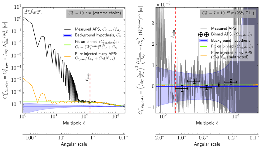
Figure 9: Illustration of the APS likelihood fit in the energy bin $[100,\,300]\,\mathrm{GeV}$. Left: Global spectrum for an extreme fluctuation of the DGRB. It can be seen how the DGRB events (orange curve) add power on the top of the shot noise from the cosmic-ray background (blue), which however is obfuscated in the data by the sky mask at $\ell\lesssim 100$ (black curve). At $\ell\gtrsim 500$, the instrumental angular resolution suppresses the intrinsic signal power to the overall shot noise level. We evaluate the spectrum at $\ell_{\rm min}\leq\ell\leq 1024$. The green curve shows the likelihood fit to the data. It can be seen that the spectrum of simulated $\gamma$-ray events alone (orange curve) is well estimated and recovered by the fit. Right: Closeup of the interval $80\leq\ell\leq 2048$ for a signal APS at the 95% C.L. sensitivity threshold, with the average shot noise power already subtracted and the beam suppression undone.

Figure 9 illustrates the analysis and the equations from section 2. In the left panel, we show an APS containing $\gamma$-ray and background events, however, for an extreme anisotropy level for illustration purpose only. To scrutinise our analysis procedure, we also show a “pure” spectrum from $\gamma$-ray events only with no cosmic-ray background (orange curve). This information is of course not available in a later analysis of real data. In the right panel, we show the APS after subtracting the shot noise and after unfolding (“signal APS”). The blue band indicates the expected unbinned error, $\sigma_{\ell}(C_{\ell,\,\rm sig}=0)$ for the background-only hypothesis. This variance band is based on the scaling $\sigma_{\ell,\,\rm raw}\approx 1.11\times\sigma_{\ell,\,\text{full-sky}}<1/\sqrt{f_{\rm sky}}\;\sigma_{\ell,\,\text{full-sky}}$ empirically derived from a set of MC simulations. The black crosses in the right panel show the signal APS with the error, Eq. 2.13, after binning and maximising the likelihood. Finally, the green curve shows the likelihood fit to the binned ${C_{\ell,\,\rm sig}}$ and in both panels well agrees with the anisotropy of the injected $N_{\gamma}$ $\gamma$-ray events (orange curves).

4.2 Results

In table 3, we present the 95% C.L. sensitivity to small-scale anisotropies in a CTA large-area survey,

$$C_{\rm P,\,95\%}^{F}=C_{\rm P,\,input}^{F}\times(N_{\gamma,\,95\%}/N_{\rm ev})^{2}\,.$$ (4.1)

In the top panel, we show the anisotropies in the total data set (including all background and DGRB events) to which CTA is sensitive to, independent of the origin of these anisotropies. While we have carefully excluded expected artefacts from the analysis in § 3.3, in principle, if any instrumental or physical origin generates anisotropies of these magnitude and on scales below $1.5{{}^{\circ}}$, they are seen by our analysis. We will later discuss in section 5 how this sensitivity can be interpreted with respect to small-scale cosmic-ray anisotropies.

Sensitivity to anisotropies in all $N_{\rm ev}$ events of the survey
Energy	“Measured” total	Fluctuation sensitivity,
interval	events, $N_{\rm ev}$	$C_{\rm P,\,95\%}^{F}\;[\rm sr]$
$[30,\,100]\,\mathrm{GeV}$	$4.99\times 10^{7}$	$(1.0\pm 0.7)\times 10^{-9}\;\,$
$[100,\,300]\,\mathrm{GeV}$	$4.21\times 10^{7}$	$(7.4\pm 4.3)\times 10^{-10}$
$[300,\,1000]\,\mathrm{GeV}$	$1.26\times 10^{7}$	$(2.1\pm 0.9)\times 10^{-9}\;\,$
$[1,\,100]\,\mathrm{TeV}$	$8.51\times 10^{6}$	$(2.8\pm 1.2)\times 10^{-9}\;\,$
$[30\,\mathrm{GeV},\,100\,\mathrm{TeV}]$	$1.13\times 10^{8}$	$(3.1\pm 2.1)\times 10^{-10}\,$

Sensitivity to anisotropies in a presumed DGRB intensity (top panel rescaled)
Energy	Presumed events	Sensitivity to	Presumed events	Sensitivity to
interval	$N_{\rm DGRB}$, Eq. 3.3	$C^{F}_{\rm P,\,DGRB}\;[\rm sr]$	$N_{\rm DGRB}$, Eq. 4.2	$C^{F}_{\rm P,\,DGRB}\;[\rm sr]$
$[30,\,100]\,\mathrm{GeV}$	$10800$	$(2.2\pm 1.5)\times 10^{-2}$	$11500$	$(2.0\pm 1.3)\times 10^{-2}$
$[100,\,300]\,\mathrm{GeV}$	$14600$	$(6.2\pm 3.6)\times 10^{-3}$	$13100$	$(7.7\pm 4.5)\times 10^{-3}$
$[300,\,1000]\,\mathrm{GeV}$	$2660$	$(4.8\pm 2.1)\times 10^{-2}$	$4400$	$(1.8\pm 0.8)\times 10^{-2}$
$[1,\,100]\,\mathrm{TeV}$	$20$	$>4\pi\,f_{\rm sky}$	$1300$	$(1.2\pm 0.5)\times 10^{-1}$
$[30\,\mathrm{GeV},\,100\,\mathrm{TeV}]$	$28100$	$(5.0\pm 3.5)\times 10^{-3}$	$30300$	$(4.3\pm 3.0)\times 10^{-3}$

Table 3: Top panel: 95% C.L. sensitivity to any anisotropies in all $N_{\rm ev}=N_{\rm bck}+N_{\rm DGRB}$ events of a $T_{\rm obs}=475\,\mathrm{h}$ CTA extragalactic survey data set. We report the median sensitivities $C_{\rm P,\,95\%}^{F}$ and, because of our analysis’ limited statistic, a symmetric 68% C.I. Bottom panel: Sensitivities to small-scale anisotropies in the DGRB for an exponentially suppressed DGRB, Eq. 3.3 (left columns) or a broken power-law extrapolation Eq. 4.2 (right columns).

In a second step, we assume that all anisotropies are generated by the $\gamma$-rays of the DGRB. Taking the results from the top panel of table 3 and some additional knowledge about the average DGRB intensity, Eq. 2.11 can be used to draw a statement about the relative fluctuation level in the DGRB detectable by our analysis. This is presented in the lower panel of table 3. Here, we show this sensitivity assuming an exponentially suppressed DGRB intensity, Eq. 3.3, on the left. While [10] have excluded a pure power-law scaling of the DGRB in the VHE regime at the $5.7\sigma$ level, they cannot distinguish between an exponential cut-off of the DGRB (suggested by the absorption of distant $\gamma$-rays on the EBL) and a continuation of the spectrum with a steeper power-law slope (which would hint to a different source class at the highest energies). Therefore, we additionally investigate our results for a broken power-law DGRB,

$$I_{\text{DGRB}}=\begin{cases}I_{\rm b}\,(E/E_{\rm b})^{-\gamma_{1}}\quad\text{if}\;E<E_{\rm b}\\ I_{\rm b}\,(E/E_{\rm b})^{-\gamma_{2}}\quad\text{otherwise,}\end{cases}$$ (4.2)

with $I_{\rm b}=5.74\times 10^{-14}\,\mathrm{cm^{-2}\,s^{-1}\,sr^{-1}\,MeV^{-1}}$, $\gamma_{1}=2.30$, $\gamma_{2}=3.07$, and $E_{\rm b}=55.3\,\mathrm{GeV}$ obtained from a fit to the Fermi-LAT data from [10, model B]. The APS sensitivity for such a broken power-law DGRB intensity is shown in the right columns of table 3. It can be seen that a power-law behaviour of the DGRB is needed in the TeV regime for generating detectable anisotropies, $C^{F}_{\rm P}\leq 4\pi\,f_{\rm sky}$ above $1\,\mathrm{TeV}$. The CTA sensitivity assuming a broken power-law extrapolation of the DGRB is finally also displayed in figure 10. We stress that an interpretation of a detected anisotropy power in terms of the DGRB relies on complementary measurements of its diffuse intensity and the corresponding expected number of CTA events.

Our results of the CTA sensitivity can be compared to the previous study from [40] using $C^{F}_{\rm P,\,DGRB}=(1-f_{\rm DM})^{2}\times C^{F}_{\rm P,\,astro}+f_{\rm DM}^{2}\times C^{F}_{\rm P,\,DM}$. The authors of [40] fixed $C^{F}_{\rm P,\,astro}\equiv 10^{-5}\,\mathrm{sr}$, $C^{F}_{\rm P,\,DM}\equiv 10^{-3}\,\mathrm{sr}$ and expressed their sensitivity in terms of the detectable fraction $f_{\rm DM}$ of dark matter induced anisotropies. With a detectable $C^{F}_{\rm P,\,DGRB}\gtrsim 4\times 10^{-3}\,\mathrm{sr}$, we find our result comparable to their most conservative assumptions about the CTA performance ($f_{\rm DM}\gtrsim 1$).

5 Discussion

DGRB anisotropies measured by the Fermi-LAT:

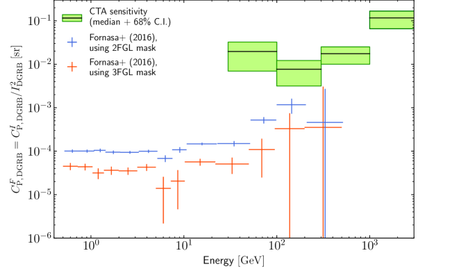
Figure 10: Sensitivity of the CTA extragalactic survey to anisotropies in the DGRB compared to the measurement by the Fermi-LAT [28]. The figure shows the relative anisotropy levels, $C^{F}_{\rm P,\,DGRB}$, with respect to the broken power-law DGRB intensity, Eq. 4.2. The highest energy bin for the CTA sensitivity shows the sensitivity integrated up to $100\,\mathrm{TeV}$.

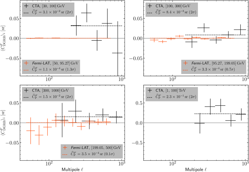
Figure 11: Comparison of the binned APS in the three overlapping bins between the Fermi-LAT analysis [28] (masking 3FGL sources) and our CTA sensitivity calculation at the 95% C.L. As in figure 10, we show the fluctuation APS with respect to the DGRB intensity of Eq. 4.2. Note that the CTA points and the fit in the upper right panel are the same as shown in figure 9 (right). Also note the larger vertical axis scale in the lower right panel.

Small-scale anisotropies in the DGRB have already been detected in the data from the Fermi-LAT. Taking 81 months of reprocessed Pass7 data between 500 MeV and 500 GeV, the authors of [28] have recently updated the earlier result from [27], based on 22 months of Fermi-LAT data. In addition to covering a larger energy range and better precision compared to the first measurement, [28] conclude on two power-law populations of point sources dominating the DGRB anisotropies below and above 2 GeV, respectively. To compare with our results, in figure 10, we show the Fermi-LAT measurement of the auto-correlation APS in terms of the fluctuation APS, $C_{\rm P,\,DGRB}^{F}$, relative to the average DGRB intensity of Eq. 4.2. The authors of [28] studied the APS for two slightly different data sets, excluding all 3FGL sources (orange crosses in figure 10) and only excluding the 2FGL sources (blue crosses). As expected, the DGRB power is reduced when masking the power originating from additionally resolved sources in the 3FGL. From the comparison between the Fermi-LAT measurement and our results, it becomes evident that the existing detection of DGRB anisotropies from [28] already weakly excludes the small-scale DGRB anisotropies accessible with CTA. However, the Fermi-LAT measurement is based on a slightly lower multipole range ($49\leq\ell\leq 706$). Also, the statistical uncertainty of the Fermi-LAT measurement in its highest energy bins is large; and in the regime of saturation of the Fermi-LAT detector, systematic biases may additionally increase the uncertainty. This is illustrated in figure 11 by a more close comparison between the three overlapping energy bins of the Fermi-LAT measurement [28] and our CTA sensitivity. Notably, a potential oversubtraction of the mask in the lowest $\ell$-bins in the Fermi-LAT measurement may artificially reduce the detected signal. We also remark that the energy APS from [28] shows low-significant features which are not yet fully understood, e.g., a peak of the angular power in the single energy bin between 50 and 95.27 GeV when using Pass8 data (which is not present for the default analysis relying on Pass7 data). Therefore, we conclude that the reach of small-scale $\gamma$-ray anisotropies with CTA is not ultimately excluded by Fermi-LAT results, in particular at the highest energies above 300 GeV, and a complementary analysis with CTA may help to reduce instrument-related systematic uncertainties.

Expected VHE anisotropy levels of various source classes:

Several estimates have been drawn to assess the expected anisotropy level from unresolved members of various source classes contributing to the DGRB [19, 31, 49, 29, 36, 58]. While this has been already extensively discussed by [27, 12], we present a short overview of these estimates together with our calculation of the CTA sensitivity in table 4. For the APS signal from Galactic DM substructure, we rely on our previous work [49], where we have comprehensively bracketed the expected intensity and APS characteristics from Galactic DM. While we have presented in figure 7 of [49] the dimensional intensity APS for a particular particle physics model, we report in table 4 $C^{F}_{\rm\ell=100}=C^{I}_{\rm\ell=100}/\langle I_{\rm DM}\rangle^{2}$ with $\langle I_{\rm DM}\rangle$ the average emission from all Galactic DM (smooth halo and subhalos) in our definition of the CTA extragalactic survey field.

Using these estimates, the second to last column in table 4 indicates the fraction of intensity of the respective source class to the DGRB to create anisotropies detectable with CTA. This is confronted with a coarse estimate of the predicted DGRB fractions (last column of table 4). It is worth noting that [17] claim that in the VHE range, $E>50\,\mathrm{GeV}$, the DGRB is dominated by the emission from unresolved blazars with $f_{\rm DGRB}=86^{+16}_{-14}\%$, although their anisotropy imprint may be too low to be detectable with CTA. A signal from Galactic DM substructure would only bear the chance of a detection for the most optimistic clustering model from [49] and the full DGRB (at the peak of the DM-induced $\gamma$-ray spectrum) originating from DM annihilation. This would apply to annihilation cross sections of $\langle\sigma v\rangle\gtrsim 10^{-23}\,\mathrm{cm^{3}\,s^{-1}}$ for DM particle masses $m_{\chi}{}\sim 1\,\mathrm{TeV}$ and annihilation into bottom quarks. Although this suggests that the indirect search for DM signals with CTA via $\gamma$-ray anisotropies is not very competitive, we stress that this conclusion only applies for the standard paradigm of weakly interacting massive dark matter particles in a $\Lambda$CDM Universe and only undergoing DM self-interactions. Moreover, a dedicated study tailored to spatially extended Galactic and extragalactic DM structures is excluded from this work. Overall, we finally conclude that an APS analysis with CTA is most promising to constrain the contribution of misaligned AGN (as already pointed out by [31]) and possibly also unresolved blazars to the DGRB in the VHE regime.

Source class	Predicted		Detectable $f_{\rm DGRB}$	Predicted $f_{\rm DGRB}$
	$C^{F}_{\rm\ell=100}\;[\rm sr]$		$(>30\,\rm GeV)$
Millisecond pulsars	$3\times 10^{-2}$	[19]	38%	$<1\%$	[20]
Misaligned AGN	$\;\,\gtrsim\;10^{-3}$ ($>100\,\mathrm{GeV}$) [31]		$\sim 1$	$\lesssim 25\%$	[14]
Galactic DM substructure (HIGH)	$3\times 10^{-4}$	[49, this work]	$\gtrsim 1$	depending on $\langle\sigma v\rangle$
Unresolved blazars	$2\times 10^{-4}$	[29]	$\gtrsim 1$	$\gtrsim 80\%$ $(>50\,\rm GeV)$	[17]
Galactic DM substructure (LOW)	$3\times 10^{-5}$	[49, this work]	$>1$	depending on $\langle\sigma v\rangle$
Extragalactic DM structure	$\gtrsim\;\;10^{-5}$	[36]	$>1$	depending on $\langle\sigma v\rangle$
Star-forming galaxies	$2\times 10^{-7}$	[58]	$>1$	$\lesssim 50\%$	[13]

Table 4: Predicted contributions to the DGRB of various unresolved source classes. If not explicitly stated, all quoted values for $C^{F}_{\ell}$ and $f_{\rm DGRB}$ are assumed constant in the $\gtrsim 100\,\mathrm{MeV}$ range. For DM annihilation, the predicted intensity depends on the velocity-averaged annihilation cross-section, $\langle\sigma v\rangle$.

Are small-scale cosmic-ray anisotropies excluded?

Throughout this paper, we have assumed a perfectly isotropised CTA residual background of electrons and misclassified hadrons. Due to the large relative amount of these background events, however, even tiny amplitudes of $C^{F}_{\rm bck}\gtrsim 10^{-9}\,\mathrm{sr}$ in the background could dominate over any $\gamma$-ray anisotropies. In fact, cosmic-ray anisotropies at scales $\gtrsim 5{{}^{\circ}}$ are since long known [59, 60], with hadronic cosmic-ray anisotropies at the level of $C^{F}_{\ell}\lesssim 10^{-9}\,\mathrm{sr}$ up to $\ell\lesssim 40$ [61, 62]. However, even when extrapolating this level beyond $\ell\gtrsim 100$, given that less than 1% of all hadrons survive the CTA $\gamma$-hadron separation cuts, remaining hadronic cosmic-ray anisotropies in the CTA background are smaller than $C^{F}_{\ell}\lesssim 10^{13}\,\mathrm{sr}$ and thus negligible.

The Fermi-LAT collaboration has recently published a search for anisotropies in the electron intensity based on almost seven years of data [63]. No electron anisotropy has been found, with an energy-dependent upper limit on the dipole anisotropy of $C_{\ell=1,\,95\%\rm C.L.}^{F}\lesssim 10^{-2}\,\mathrm{sr}$. As their analysis suggests a sensitivity to $C^{F}_{\ell}\lesssim 10^{-6}\,\mathrm{sr}$ at $\ell\geq 100$ and $E\geq 100\,\mathrm{GeV}$, it remains to comprehensively study whether CTA’s sensitivity to small-scale anisotropies may supersede Fermi-LAT’s ability to measure electron anisotropies at $\ell\gtrsim 100$.

However, although low-amplitude small-scale electron anisotropies may be within CTA’s sensitivity range, we judge their existence to be highly unlikely. Only primary cosmic electrons, accelerated in point-like sources and with sufficiently large Larmor-radii, are able to generate small-scale anisotropies. Because of their fast synchrotron cooling, such primary electrons must originate from nearby ($d\lesssim 1\,\mathrm{kpc}$) sources, and only a few supernova remnants constitute plausible candidates [64]. Also, the scenario of DM annihilation in nearby subhalos generating electron anisotropies is considered to be already ruled out [65, 66].

6 Conclusions

In this work, we have studied whether CTA is able to probe small-scale anisotropies in the DGRB, based on the latest knowledge about the future instrument. Using standard background rejection cuts and a binned likelihood analysis, we have found a sensitivity to $\gamma$-ray anisotropies with relative amplitudes of $C^{F}_{\rm P,\,DGRB}\gtrsim 4\times 10^{-3}\,\mathrm{sr}$ above 30 GeV and scales smaller than $1.5{{}^{\circ}}$. Beyond $1\,\mathrm{TeV}$, such anisotropies may only be detectable if the DGRB is not exponentially suppressed at sub-TeV energies. While small-scale anisotropies are most likely solely generated by $\gamma$-rays, our results can also be interpreted in terms of any anisotropies present in the data, to which our results show a sensitivity to $C^{F}_{\rm P}\gtrsim 3\times 10^{-10}\,\mathrm{sr}$.

We have confronted this sensitivity to previous detections of DGRB anisotropies in the Fermi-LAT data. CTA may be in reach to detect the anisotropy levels found at low significance by the Fermi-LAT, in particular at $\gamma$-ray energies above 300 GeV. A complementary analysis of CTA data may also help to rule out systematic biases affecting the current and future [67] Fermi-LAT measurements. Discussing various classes of unresolved astrophysical $\gamma$-ray emitters, a CTA analysis of VHE $\gamma$-ray anisotropies will be primarily able to probe current models for the population of unresolved blazars and misaligned AGN.

Investigating various anticipated CTA data sets, we have found the CTA extragalactic survey to be most suitable for this kind of analysis; and the analysis presented in this paper proposes an additional way of studying the survey data. On the other hand, we have stated that the analysis of single-FOV data for a non-Gaussian acceptance of the instrument is heavily impeded by artefacts in the multipole transformation. Discussing various sources of pollution to an ideal survey data set, we have obtained that a homogeneous exposure is most crucial for the success of the search for small-scale anisotropies. We therefore recommend a survey tiling as small as $1{{}^{\circ}}$ or even a slew survey, where data is taken continuously. Whether the sensitivity of CTA to $\gamma$-ray anisotropies can be further improved by such a slew survey (at the potential expense of a worse angular resolution), using divergent telescope pointing, dedicated analysis cuts, or a sophisticated modelling of the background APS, is finally left to future work.

References

- [1] W. B. Atwood, A. A. Abdo, M. Ackermann, W. Althouse, B. Anderson, M. Axelsson et al., The Large Area Telescope on the Fermi Gamma-Ray Space Telescope Mission, ApJ 697 (June, 2009) 1071–1102, [0902.1089].
- [2] F. Acero, M. Ackermann, M. Ajello, A. Albert, W. B. Atwood, M. Axelsson et al., Fermi Large Area Telescope Third Source Catalog, ApJS 218 (June, 2015) 23, [1501.02003].
- [3] S. P. Wakely and D. Horan, TeVCat: An online catalog for Very High Energy Gamma-Ray Astronomy, International Cosmic Ray Conference 3 (2008) 1341–1344.
- [4] W. L. Kraushaar, G. W. Clark, G. P. Garmire, R. Borken, P. Higbie, V. Leong et al., High-Energy Cosmic Gamma-Ray Observations from the OSO-3 Satellite, ApJ 177 (Nov., 1972) 341.
- [5] C. E. Fichtel, R. C. Hartman, D. A. Kniffen, D. J. Thompson, G. F. Bignami, H. Ögelman et al., High-energy gamma-ray results from the second small astronomy satellite, ApJ 198 (May, 1975) 163–182.
- [6] M. Ackermann, M. Ajello, W. B. Atwood, L. Baldini, J. Ballet, G. Barbiellini et al., Fermi-LAT Observations of the Diffuse -Ray Emission: Implications for Cosmic Rays and the Interstellar Medium, ApJ 750 (May, 2012) 3, [1202.4039].
- [7] M. Su, T. R. Slatyer and D. P. Finkbeiner, Giant Gamma-ray Bubbles from Fermi-LAT: Active Galactic Nucleus Activity or Bipolar Galactic Wind?, ApJ 724 (Dec., 2010) 1044–1082, [1005.5480].
- [8] J.-M. Casandjian, I. Grenier and for the Fermi Large Area Telescope Collaboration, High Energy Gamma-Ray Emission from the Loop I region, ArXiv e-prints (Dec., 2009) , [0912.3478].
- [9] A. A. Abdo, M. Ackermann, M. Ajello, W. B. Atwood, L. Baldini, J. Ballet et al., Spectrum of the Isotropic Diffuse Gamma-Ray Emission Derived from First-Year Fermi Large Area Telescope Data, Phys. Rev. Lett. 104 (Mar., 2010) 101101, [1002.3603].
- [10] M. Ackermann, M. Ajello, A. Albert, W. B. Atwood, L. Baldini, J. Ballet et al., The Spectrum of Isotropic Diffuse Gamma-Ray Emission between 100 MeV and 820 GeV, ApJ 799 (Jan., 2015) 86, [1410.3696].
- [11] C. D. Dermer, The Extragalactic -ray Background, in The First GLAST Symposium (S. Ritz, P. Michelson and C. A. Meegan, eds.), vol. 921 of American Institute of Physics Conference Series, pp. 122–126, July, 2007. 0704.2888. DOI.
- [12] M. Fornasa and M. A. Sánchez-Conde, The nature of the Diffuse Gamma-Ray Background, Phys. Rep. 598 (Oct., 2015) 1–58, [1502.02866].
- [13] I. Tamborra, S. Ando and K. Murase, Star-forming galaxies as the origin of diffuse high-energy backgrounds: gamma-ray and neutrino connections, and implications for starburst history, J. Cosmology Astropart. Phys. 09 (Sept., 2014) 043, [1404.1189].
- [14] M. Di Mauro, F. Calore, F. Donato, M. Ajello and L. Latronico, Diffuse -Ray Emission from Misaligned Active Galactic Nuclei, ApJ 780 (Jan., 2014) 161, [1304.0908].
- [15] M. Di Mauro and F. Donato, Composition of the Fermi-LAT isotropic gamma-ray background intensity: Emission from extragalactic point sources and dark matter annihilations, Phys. Rev. D 91 (June, 2015) 123001, [1501.05316].
- [16] M. Ajello, D. Gasparrini, M. Sánchez-Conde, G. Zaharijas, M. Gustafsson, J. Cohen-Tanugi et al., The Origin of the Extragalactic Gamma-Ray Background and Implications for Dark Matter Annihilation, ApJ 800 (Feb., 2015) L27, [1501.05301].
- [17] M. Ackermann, M. Ajello, A. Albert, W. B. Atwood, L. Baldini, J. Ballet et al., Resolving the Extragalactic -ray Background above 50 GeV with the Fermi Large Area Telescope, Phys. Rev. Lett. 116 (Apr., 2016) 151105, [1511.00693].
- [18] M. Di Mauro, S. Manconi, H.-S. Zechlin, M. Ajello, E. Charles and F. Donato, Deriving the Contribution of Blazars to the Fermi-LAT Extragalactic -ray Background at GeV with Efficiency Corrections and Photon Statistics, ApJ 856 (Apr., 2018) 106, [1711.03111].
- [19] J. M. Siegal-Gaskins, R. Reesman, V. Pavlidou, S. Profumo and T. P. Walker, Anisotropies in the gamma-ray sky from millisecond pulsars, MNRAS 415 (Aug., 2011) 1074–1082, [1011.5501].
- [20] F. Calore, M. Di Mauro and F. Donato, Diffuse -Ray Emission from Galactic Pulsars, ApJ 796 (Nov., 2014) 14, [1406.2706].
- [21] J. E. Gunn, B. W. Lee, I. Lerche, D. N. Schramm and G. Steigman, Some astrophysical consequences of the existence of a heavy stable neutral lepton, ApJ 223 (Aug., 1978) 1015–1031.
- [22] F. W. Stecker, The cosmic -ray background from the annihilation of primordial stable neutral heavy leptons, ApJ 223 (Aug., 1978) 1032–1036.
- [23] M. Hütten, C. Combet and D. Maurin, Extragalactic diffuse -rays from dark matter annihilation: revised prediction and full modelling uncertainties, J. Cosmology Astropart. Phys. 2 (Feb., 2018) 005, [1711.08323].
- [24] V. Khaire and R. Srianand, Star Formation History, Dust Attenuation, and Extragalactic Background Light, ApJ 805 (May, 2015) 33, [1405.7038].
- [25] A. Franceschini, G. Rodighiero and M. Vaccari, Extragalactic optical-infrared background radiation, its time evolution and the cosmic photon-photon opacity, A&A 487 (Sept., 2008) 837–852, [0805.1841].
- [26] M. Ackermann, M. Ajello, W. B. Atwood, L. Baldini, J. Ballet, G. Barbiellini et al., 2FHL: The Second Catalog of Hard Fermi-LAT Sources, ApJS 222 (Jan., 2016) 5, [1508.04449].
- [27] M. Ackermann, M. Ajello, A. Albert, L. Baldini, J. Ballet, G. Barbiellini et al., Anisotropies in the diffuse gamma-ray background measured by the Fermi LAT, Phys. Rev. D 85 (Apr., 2012) 083007, [1202.2856].
- [28] M. Fornasa, A. Cuoco, J. Zavala, J. M. Gaskins, M. A. Sánchez-Conde, G. Gomez-Vargas et al., Angular power spectrum of the diffuse gamma-ray emission as measured by the Fermi Large Area Telescope and constraints on its dark matter interpretation, Phys. Rev. D 94 (Dec., 2016) 123005, [1608.07289].
- [29] S. Ando, E. Komatsu, T. Narumoto and T. Totani, Dark matter annihilation or unresolved astrophysical sources? Anisotropy probe of the origin of the cosmic gamma-ray background, Phys. Rev. D 75 (Mar., 2007) 063519, [astro-ph/0612467].
- [30] A. Cuoco, E. Komatsu and J. M. Siegal-Gaskins, Joint anisotropy and source count constraints on the contribution of blazars to the diffuse gamma-ray background, Phys. Rev. D 86 (Sept., 2012) 063004, [1202.5309].
- [31] M. Di Mauro, A. Cuoco, F. Donato and J. M. Siegal-Gaskins, Fermi-LAT -ray anisotropy and intensity explained by unresolved radio-loud active galactic nuclei, J. Cosmology Astropart. Phys. 11 (Nov., 2014) 021, [1407.3275].
- [32] S. Ando and E. Komatsu, Anisotropy of the cosmic gamma-ray background from dark matter annihilation, Phys. Rev. D 73 (Jan., 2006) 023521, [astro-ph/0512217].
- [33] J. M. Siegal-Gaskins, Revealing dark matter substructure with anisotropies in the diffuse gamma-ray background, J. Cosmology Astropart. Phys. 10 (Oct., 2008) 040, [0807.1328].
- [34] M. Fornasa, L. Pieri, G. Bertone and E. Branchini, Anisotropy probe of galactic and extra-galactic dark matter annihilations, Phys. Rev. D 80 (July, 2009) 023518, [0901.2921].
- [35] A. Cuoco, A. Sellerholm, J. Conrad and S. Hannestad, Anisotropies in the diffuse gamma-ray background from dark matter with Fermi LAT: a closer look, MNRAS 414 (July, 2011) 2040–2054, [1005.0843].
- [36] M. Fornasa, J. Zavala, M. A. Sánchez-Conde, J. M. Siegal-Gaskins, T. Delahaye, F. Prada et al., Characterization of dark-matter-induced anisotropies in the diffuse gamma-ray background, MNRAS 429 (Feb., 2013) 1529–1553, [1207.0502].
- [37] S. Ando and E. Komatsu, Constraints on the annihilation cross section of dark matter particles from anisotropies in the diffuse gamma-ray background measured with Fermi-LAT, Phys. Rev. D 87 (June, 2013) 123539, [1301.5901].
- [38] G. A. Gómez-Vargas, A. Cuoco, T. Linden, M. A. Sánchez-Conde, J. M. Siegal-Gaskins, T. Delahaye et al., Dark matter implications of Fermi-LAT measurement of anisotropies in the diffuse gamma-ray background, Nucl. Instr. Meth. Phys. Res. A 742 (Apr., 2014) 149–153, [1303.2154].
- [39] J. U. Lange and M.-C. Chu, Can galactic dark matter substructure contribute to the cosmic gamma-ray anisotropy?, MNRAS 447 (Feb., 2015) 939–947, [1412.5749].
- [40] J. Ripken, A. Cuoco, H.-S. Zechlin, J. Conrad and D. Horns, The sensitivity of Cherenkov telescopes to dark matter and astrophysical anisotropies in the diffuse gamma-ray background, J. Cosmology Astropart. Phys. 1 (Jan., 2014) 049, [1211.6922].
- [41] B. S. Acharya, M. Actis, T. Aghajani, G. Agnetta, J. Aguilar, F. Aharonian et al., Introducing the CTA concept, Astropart. Phys. 43 (Mar., 2013) 3–18.
- [42] B. S. Acharya, I. Agudo, I. A. Samarai, R. Alfaro, J. Alfaro, C. Alispach et al., Science with the Cherenkov Telescope Array, ArXiv e-prints (Sept., 2017) , [1709.07997].
- [43] L. Knox, Determination of inflationary observables by cosmic microwave background anisotropy experiments, Phys. Rev. D 52 (Oct., 1995) 4307–4318, [astro-ph/9504054].
- [44] B. D. Wandelt, E. Hivon and K. M. Górski, Cosmic microwave background anisotropy power spectrum statistics for high precision cosmology, Phys. Rev. D 64 (Oct., 2001) 083003, [astro-ph/0008111].
- [45] E. Komatsu, B. D. Wandelt, D. N. Spergel, A. J. Banday and K. M. Górski, Measurement of the Cosmic Microwave Background Bispectrum on the COBE DMR Sky Maps, ApJ 566 (Feb., 2002) 19–29, [astro-ph/0107605].
- [46] T. Poutanen, D. Maino, H. Kurki-Suonio, E. Keihänen and E. Hivon, Cosmic microwave background power spectrum estimation with the destriping technique, MNRAS 353 (Sept., 2004) 43–58, [astro-ph/0404134].
- [47] S. Ando, Gamma-ray background anisotropy from Galactic dark matter substructure, Phys. Rev. D 80 (July, 2009) 023520, [0903.4685].
- [48] F. Calore, V. De Romeri, M. Di Mauro, F. Donato, J. Herpich, A. V. Macciò et al., -ray anisotropies from dark matter in the Milky Way: the role of the radial distribution, MNRAS 442 (Aug., 2014) 1151–1156, [1402.0512].
- [49] M. Hütten, C. Combet, G. Maier and D. Maurin, Dark matter substructure modelling and sensitivity of the Cherenkov Telescope Array to Galactic dark halos, J. Cosmology Astropart. Phys. 9 (Sept., 2016) 047, [1606.04898].
- [50] G. Dubus, J. L. Contreras, S. Funk, Y. Gallant, T. Hassan, J. Hinton et al., Surveys with the Cherenkov Telescope Array, Astropart. Phys. 43 (Mar., 2013) 317–330, [1208.5686].
- [51] J. Knödlseder, M. Mayer, C. Deil, J.-B. Cayrou, E. Owen, N. Kelley-Hoskins et al., GammaLib and ctools. A software framework for the analysis of astronomical gamma-ray data, A&A 593 (Aug., 2016) A1, [1606.00393].
- [52] K. M. Górski, E. Hivon, A. J. Banday, B. D. Wandelt, F. K. Hansen, M. Reinecke et al., HEALPix: A Framework for High-Resolution Discretization and Fast Analysis of Data Distributed on the Sphere, ApJ 622 (Apr., 2005) 759–771, [astro-ph/0409513].
- [53] G. Cowan, K. Cranmer, E. Gross and O. Vitells, Asymptotic formulae for likelihood-based tests of new physics, European Physical Journal C 71 (Feb., 2011) 1554, [1007.1727].
- [54] I. Szapudi, S. Prunet, D. Pogosyan, A. S. Szalay and J. R. Bond, Fast Cosmic Microwave Background Analyses via Correlation Functions, ApJ 548 (Feb., 2001) L115–L118.
- [55] A. Challinor, G. Chon, S. Colombi, E. Hivon, S. Prunet and I. Szapudi, “PolSpice: Spatially Inhomogeneous Correlation Estimator for Temperature and Polarisation.” Astrophysics Source Code Library, Sept., 2011.
- [56] E. Hivon, K. M. Górski, C. B. Netterfield, B. P. Crill, S. Prunet and F. Hansen, MASTER of the Cosmic Microwave Background Anisotropy Power Spectrum: A Fast Method for Statistical Analysis of Large and Complex Cosmic Microwave Background Data Sets, ApJ 567 (Mar., 2002) 2–17, [astro-ph/0105302].
- [57] S. S. Campbell, Angular power spectra with finite counts, MNRAS 448 (Apr., 2015) 2854–2878, [1411.4031].
- [58] S. Ando and V. Pavlidou, Imprint of galaxy clustering in the cosmic gamma-ray background, MNRAS 400 (Dec., 2009) 2122–2127, [0908.3890].
- [59] M. Amenomori, S. Ayabe, S. W. Cui, Danzengluobu, L. K. Ding, X. H. Ding et al., Large-Scale Sidereal Anisotropy of Galactic Cosmic-Ray Intensity Observed by the Tibet Air Shower Array, ApJ 626 (June, 2005) L29–L32, [astro-ph/0505114].
- [60] A. A. Abdo, B. T. Allen, T. Aune, D. Berley, S. Casanova, C. Chen et al., The Large-Scale Cosmic-Ray Anisotropy as Observed with Milagro, ApJ 698 (June, 2009) 2121–2130, [0806.2293].
- [61] The HAWC Collaboration and The IceCube Collaboration, Full-Sky Analysis of Cosmic-Ray Anisotropy with IceCube and HAWC, ArXiv e-prints (Oct., 2015) , [1510.04134].
- [62] The HAWC Collaboration and The IceCube Collaboration, Combined Analysis of Cosmic-Ray Anisotropy with IceCube and HAWC, ArXiv e-prints (Aug., 2017) , [1708.03005].
- [63] S. Abdollahi, M. Ackermann, M. Ajello, A. Albert, W. B. Atwood, L. Baldini et al., Search for Cosmic-Ray Electron and Positron Anisotropies with Seven Years of Fermi Large Area Telescope Data, Phys. Rev. Lett. 118 (Mar., 2017) 091103, [1703.01073].
- [64] X. Li, Z.-Q. Shen, B.-Q. Lu, T.-K. Dong, Y.-Z. Fan, L. Feng et al., ‘Excess’ of primary cosmic ray electrons, Physics Letters B 749 (Oct., 2015) 267–271, [1412.1550].
- [65] E. Borriello, L. Maccione and A. Cuoco, Dark matter electron anisotropy: A universal upper limit, Astroparticle Physics 35 (Mar., 2012) 537–546, [1012.0041].
- [66] S. Profumo, An observable electron-positron anisotropy cannot be generated by dark matter, J. Cosmology Astropart. Phys. 2 (Feb., 2015) 043, [1405.4884].
- [67] M. Negro for the Fermi-LAT Collaboration, Study of the anisotropy of the unresolved gamma-ray background, in Proceedings of the 7th International Fermi Symposium, p. 158, Oct., 2017.