Classical polymerization of the Schwarzschild metric

Abstract

We study a spherically symmetric setup consisting of a Schwarzschild metric as the background geometry in the framework of classical polymerization. This process is an extension of the polymeric representation of quantum mechanics in such a way that a transformation maps classical variables to their polymeric counterpart. We show that the usual Schwarzschild metric can be extracted from a Hamiltonian function which in turn, gets modifications due to the classical polymerization. Then, the polymer corrected Schwarzschild metric may be obtained by solving the polymer-Hamiltonian equations of motion. It is shown that while the conventional Schwarzschild space-time is a vacuum solution of the Einstein equations, its polymer-corrected version corresponds to an energy-momentum tensor that exhibits the features of dark energy. We also use the resulting metric to investigate some thermodynamical quantities associated to the Schwarzschild black hole, and in comparison with the standard Schwarzschild metric the similarities and differences are discussed.
PACS numbers: 04.70.Dy, 04.60.Kz, 04.60.Nc
Keywords: Classical polymerization; Schwarzschild black hole

1 Introduction

One of the most important arenas that shows the power of general relativity in describing the gravitational phenomena is the classical theory of black hole physics. However, when we introduce the quantum considerations to study of a gravitational systems, general relativity does not provide a satisfactory description of the physics of the system. The Phenomena such as black hole radiation and all kinds of cosmological singularities are among the phenomena in which the use of quantum mechanics in their description is inevitable. This means that although general relativity is a classical theory, in its most important applications, the system under consideration originally obeys the rules of quantum mechanics. Therefore, any hope in the accurate description of gravitational systems in high energies depends on the development of a complete theory of quantum gravity. That is why the quantum gravity is one of the most important challenges in theoretical physics which from its DeWitt’s traditional canonical formulation [1] to the more modern viewpoints of string theory and loop quantum gravity (LQG) [2]-[4] has gone a long way. One of the main features of the space-time proposed in LQG is its granular structure which in turn, supports the idea of existence of a minimal measurable length. In the absence of a full theory of quantum gravity, effective theories which somehow exhibits quantum effects in gravitational systems play a significant role. These are theories which show some phenomenological aspects of quantum gravity and usually use a certain deformation in their formalism. For example, theories like generalized uncertainty principles and noncommutative geometry are is this category [5]-[8].

Among the effective theories that also use a minimal length scale in their formalism, we can mention the polymer quantization [9], which uses the methods very similar to the effective theories of LQG [10]. In polymer quantum approach a polymer length scale, $\lambda$, which shows the scale of the segments of the granular space enters into the Hamiltonian of the system to deform its functional form into a so-called polymeric Hamiltonian. This means that in a polymeric quantized system in addition of a quantum parameter $\hbar$, which is responsible to canonical quantization of the system, there is also another quantum parameter $\lambda$, that labels the granular properties of the underlying space. This approach then opened a new windows for the theories which are dealing with the quantum gravitational effects in physical systems such as quantum cosmology and black hole physics, see for instance [11] and [12] and the references therein.

To polymerize a dynamical system one usually begins with a classical system described by Hamiltonian $H$. The canonical quantization of such a system transforms its Hamiltonian to an Hermitian operator, which now contains the parameter $\hbar$, in such a way that in the limit $\hbar\rightarrow 0$, the quantum Hamiltonian $H_{\hbar}$ returns to its classical counterpart. By polymerization, the Hamiltonian gets an additional quantum parameter $\lambda$, which is rooted in the ideas of granular structure of the space-time. Therefore, by taking the classical limit of the resulting Hamiltonian $H_{\hbar,\lambda}$, we arrive at a semi-classical theory in which the parameter $\lambda$ is still present. To achieve the initial classical theory, one should once again take the limit $\lambda\rightarrow 0$ from this intermediate theory. It is believed that such an effective classical theories $H_{\lambda}$, have enough rich structure to exhibit some important features of the system related to the quantum effects without quantization of the system. The process by which the theory $H_{\lambda}$ is obtained from the classical theory is called classical polymerization. A detailed explanation of this process with some of its cosmological applications can be found in [13].

In this paper, we are going to study how the metric of the Schwarzschild black hole gets modifications due to the classical polymerization. Since the thermodynamical properties of the black hole come from its geometrical structure, the corrections to the black hole’s geometry yield naturally modifications to its thermodynamics. To do this, we begin with a general form of a spherically symmetric space-time and then construct a Hamiltonian in such a way that the Schwarzschild metric is resulted from the corresponding Hamiltonian equations of motion. We then follow the the procedure described above and by application it to the mentioned Hamiltonian we get the classical polymerized Hamiltonian, by means of which we expect to obtain the polymer-corrected Schwarzschild metric. The paper is organized as follows. In section 2 we have presented a brief review of the polymer representation and classical polymerization. Section 3 is devoted to the Hamiltonian formalism of a general spherically symmetric space time. We show in this section that the resulting Hamiltonian equations of motion yield the Schwarzschild solution. In section 4, we will apply the classical polymerization on the Hamiltonian of the spherically symmetric space-time given in section 3 to get the polymerized Hamiltonian. We then construct the deformed Hamiltonian equations of motion and solve them to arrive the polymer corrected Schwarzschild metric. The energy-momentum tensor of the matter field corresponding to this metric as well as some of its thermodynamical properties are also presented in this section. The radial geodesics of the light and particles are obtained in section 5 and finally, we summarize the results in section 6.

2 Classical polymerization: a brief review

As is well-known, in Schrödinger picture of quantum mechanics, the coordinates and momentum representations are equivalent and may be easily converted to each other by a Fourier transformation. However, in the presence of the quantum gravitational effects the space-time may take a discrete structure so that such a well-defined representations are no longer applicable. As an alternative, polymer quantization provides a suitable framework for studying these situations [9, 10]. The Hilbert space of this representation of quantum mechanics is ${\mathcal{H}}_{\rm poly}=L^{2}(R_{{}_{d}},d\mu_{{}_{d}})$, where $d\mu_{{}_{d}}$ is the Haar measure, and $R_{{}_{d}}$ denotes the real discrete line whose segments are labeled by an extra dimension-full parameter $\lambda$ such that the standard Schrödinger picture will be recovered in the continuum limit $\lambda\rightarrow\ 0$. This means that by a classical limit $\hbar\rightarrow\,0$, the polymer quantum mechanics tends to an effective $\lambda$-dependent classical theory which is somehow different from the classical theory from which we have started. Such an effective theory may also be obtained directly from the standard classical theory, without referring to the polymer quantization, by using of the Weyl operator [13]. The process is known as polymerization with which we will deal in the rest of this paper.

According to the mentioned above form of the Hilbert space of the polymer representation of quantum mechanics, the position space (with coordinate $q$) has a discrete structure with discreteness parameter $\lambda$. Therefore, the associated momentum operator $\hat{p}$, which is the generator of the displacement, does not exist [10]. However, the Weyl exponential operator (shift operator) correspond to the discrete translation along $q$ is well defined and effectively plays the role of momentum associated to $q$ [9]. This allows us to utilize the Weyl operator to find an effective momentum in the semiclassical regime. So, consider a state $f(q)$, its derivative with respect to the discrete position $q$ may be approximated by means of the Weyl operator as [13]

$$\partial_{q}f(q)\approx\frac{1}{2\lambda}[f(q+\lambda)-f(q-\lambda)]\hskip 56.9055pt$$

$$=\frac{1}{2\lambda}\Big{(}\widehat{e^{ip\lambda}}-\widehat{e^{-ip\lambda}}\Big{)}\,f(q)=\frac{i}{\lambda}\widehat{\sin(\lambda p)}\,f(q),$$ (1)

and similarly the second derivative approximation will be

$$\partial_{q}^{2}f(q)\approx\frac{1}{\lambda^{2}}[f(q+\lambda)-2f(q)+f(q-\lambda)]\hskip 28.45274pt$$

$$=\frac{2}{\lambda^{2}}(\widehat{\cos(\lambda p)}-1)\,f(q).\hskip 56.9055pt$$ (2)

Having the above approximations at hand, we define the polymerization process for the finite values of the parameter $\lambda$ as

$$\hat{p}\rightarrow\,\frac{1}{\lambda}\widehat{\sin(\lambda p)},\hskip 28.45274pt\hat{p}^{2}\rightarrow\,\frac{2}{\lambda^{2}}(1-\widehat{\cos(\lambda p)}).$$ (3)

This replacements suggest the idea that a classical theory may be obtained via this process, but now without any attribution to the Weyl operator. This is what which is dubbed usually as classical Polymerization in literature [9, 13]:

$$q\rightarrow q,\hskip 42.67912ptp\rightarrow\frac{\sin(\lambda p)}{\lambda},\hskip 14.22636ptp^{2}\rightarrow\frac{2}{\lambda^{2}}\left[1-\cos(\lambda p)\right],$$ (4)

where now $(q,p)$ are a pair of classical phase space variables. Hence, by applying the transformation (4) to the Hamiltonian of a classical system we get its classical polymerized counterpart. A glance at (4) shows that the momentum is periodic and varies in a bounded interval as $p\in[-\frac{\pi}{\lambda},+\frac{\pi}{\lambda})$. In the limit $\lambda\rightarrow\,0$, one recovers the usual range for the canonical momentum $p\in(-\infty,+\infty)$. Therefore, the polymerized momentum is compactified and topology of the momentum sector of the phase space is $S^{1}$ rather than the usual $R$ [14]. Our set-up to explain the classical polymerization of a dynamical system is now complete. In section 4, we will return to this issue by some more explanations and apply it to the Hamiltonian dynamics of a spherically symmetric space-time.

3 Hamiltonian model of the spherically symmetric space-time

We start with the general spherically symmetric line element as [15]

$$ds^{2}=-a(r)dt^{2}+N(r)dr^{2}+2B(r)dtdr+b^{2}(r)\left(d\vartheta^{2}+\sin^{2}\vartheta d\varphi^{2}\right),$$ (5)

where $a(r)$, $B(r)$, $N(r)$ and $b(r)$ are some functions of $r$. Upon substitution this metric into the Einstein-Hilbert action

$${\cal S}=\frac{1}{16\pi G}\int d^{4}x\sqrt{-g}{\cal R},$$ (6)

the action takes the form

$${\cal S}=\int dt\int drL(a,b,n),$$ (7)

where [15]

$$L=2\sqrt{n}\left(\frac{a^{\prime}b^{\prime}b}{n}+\frac{ab^{\prime 2}}{n}+1\right),$$ (8)

is an effective Lagrangian in which the primes denote differentiation with respect to $r$ and the Lagrange multiplier $n$ is given by

$$n(r)=a(r)N(r)+B^{2}(r).$$ (9)

In metric (5) the function $N(r)$ plays the role of a lapse function with respect to the $r$-slicing in the ADM terminology, see [15] and [16]. On the other hand, according to the relation (9), the functions $N$ and $B$ are related to the Lagrange multiplier $n$ which means that we can arbitrarily choose them. This is a reflection of this fact that we have freedom in the definition of the coordinates $r$ and $t$ in the metric (5). Hence, the only independent variables that can be determined by the Einstein field equations are the functions $a(r)$ and $b(r)$. In order to write the Hamiltonian the momenta conjugate to these variables should be evaluated, that is

$$p_{a}=\frac{\partial L}{\partial a^{\prime}}=\frac{2bb^{\prime}}{\sqrt{n}},\hskip 14.22636ptp_{b}=\frac{\partial L}{\partial b^{\prime}}=2\frac{(2ab^{\prime}+a^{\prime}b)}{\sqrt{n}}.$$ (10)

Also, the momentum associated to $n$ vanishes which gives the primary constraint

$$p_{n}=\frac{\partial L}{\partial n^{\prime}}=0.$$ (11)

In terms of these conjugate momenta the canonical Hamiltonian is given by its standard definition $H=\sum_{q=a,b,n}q^{\prime}p_{q}-L$, leading to

$$H=\sqrt{n}\left(\frac{p_{a}p_{b}}{2b}-\frac{a}{2b^{2}}p_{a}^{2}-2\right)+\Lambda p_{n},$$ (12)

in which due to existence of the constraint (11), we have added the last term that is the primary constraints multiplied by an arbitrary functions $\Lambda(r)$. The Hamiltonian equation for $n$ then reads

$$n^{\prime}=\{n,H\}=\Lambda.$$ (13)

Now, let us restrict ourselves to a certain class of gauges, namely $n=\mbox{const.}$, which is equivalent to the choice $\Lambda=0$. With a constant $n$ we assume $n=1$ without losing general character of the solutions. By this choice, the Hamiltonian equations of motion for the other variables are as

$$\left\{\begin{array}[]{ll}a^{\prime}=\{a,H\}=\frac{p_{b}}{2b}-\frac{a}{b^{2}}p_{a},\\ \\ p^{\prime}_{a}=\{p_{a},H\}=\frac{p_{a}^{2}}{2b^{2}},\\ \\ b^{\prime}=\{b,H\}=\frac{p_{a}}{2b},\\ \\ p^{\prime}_{b}=\{p_{b},H\}=\frac{p_{a}p_{b}}{2b^{2}}-\frac{a}{b^{3}}p_{a}^{2}.\end{array}\right.$$ (21)

From the second and third equations of (21) we obtain

$$p_{a}=k_{1}b,$$ (22)

from which one gets

$$b(r)=\frac{k_{1}}{2}r+k_{2},\hskip 14.22636ptp_{a}(r)=\frac{k_{1}^{2}}{2}r+k_{1}k_{2},$$ (23)

where $k_{1}$ and $k_{2}$ are integration constants. Upon substitution these results into the first and fourth equations of (21) we arrive at the system

$$\left\{\begin{array}[]{ll}a^{\prime}=\frac{1}{k_{1}r+2k_{2}}p_{b}-\frac{2k_{1}}{k_{1}r+2k_{2}}a,\\ \\ p^{\prime}_{b}=\frac{k_{1}}{k_{1}r+2k_{2}}p_{b}-\frac{2k_{1}^{2}}{k_{1}r+2k_{2}}a,\end{array}\right.$$ (27)

which results $p^{\prime}_{b}=k_{1}a^{\prime}$ and then $p_{b}=k_{1}a+k_{3}$. Therefore,

$$a^{\prime}(r)=-\frac{k_{1}a+k_{3}}{k_{1}r+2k_{2}},$$ (28)

which after integration we obtain

$$a(r)=\frac{k_{3}}{k_{1}}+\frac{k_{1}k_{4}}{k_{1}r+2k_{2}},$$ (29)

and

$$p_{b}(r)=2k_{3}+\frac{k_{1}^{2}k_{4}}{k_{1}r+2k_{2}},$$ (30)

with $k_{3}$ and $k_{4}$ being integration constants. Now, all of the above results should satisfy the constraint equation $H=0$. Thus, with the help of (12) we get $k_{1}k_{3}=4$, where we fix them as $k_{1}=k_{3}=2$. Also, $k_{2}$ and $k_{4}$ remain arbitrary where we take their values as $k_{2}=0$ and $k_{4}=-2M$ with $M$ being a constant. Therefore, the metric functions take the form

$$a(r)=1-\frac{2M}{r},\hskip 14.22636ptb(r)=r,$$ (31)

and their conjugate momenta are

$$p_{a}(r)=2r,\hskip 14.22636ptp_{b}(r)=4-\frac{4M}{r}.$$ (32)

Finally, with using these relations in (5) and (9), the metric is obtained as

$$ds^{2}=-\left(1-\frac{2M}{r}\right)dt^{2}+N(r)dr^{2}+2\left[1-\left(1-\frac{2M}{r}\right)N(r)\right]^{1/2}dtdr+r^{2}\left(d\vartheta^{2}+\sin^{2}\vartheta d\varphi^{2}\right).$$ (33)

In the final stage we have to eliminate the function $N(r)$. This function should be interpreted as a Lagrange-multiplier and thus, cannot be considered as a real dynamical variable. As we mentioned before, one may freely chooses it. From the physical point of view the function $N(r)$ corresponds to a gauge freedom in choice of coordinates $r$ and $t$ in the above metric. If we choose the lapse function as $N(r)=\left(1-\frac{2M}{r}\right)^{-1}$ this metric takes its canonical form

$$ds^{2}=-\left(1-\frac{2M}{r}\right)dt^{2}+\left(1-\frac{2M}{r}\right)^{-1}dr^{2}+r^{2}\left(d\vartheta^{2}+\sin^{2}\vartheta d\varphi^{2}\right),$$ (34)

which is nothing but the familiar form for the metric of the Schwarzschild black hole. However, we may identify the line element (33) with the Eddington-Finkelstein metric

$$ds^{2}=-\left(1-\frac{2M}{r}\right)dt^{2}+\frac{4M}{r}dtdr+\left(1+\frac{2M}{r}\right)dr^{2}+r^{2}\left(d\vartheta^{2}+\sin^{2}\vartheta d\varphi^{2}\right),$$ (35)

for $N(r)=1+2M/r$, or with some other kinds of spherically symmetric metrics for $N=1$, see [17]. In summary, from physical viewpoint choosing different gauge functions $N(r)$ is actually looking at a space-time from a different perspective. For example, the metric (35) can be obtained from (34) by introducing a new time coordinate $\bar{t}=t+2M\ln(r-2M)$ in which the radial null geodesics (see section 5) become straight lines. In this sense, the two metrics may differ from some aspects. While the Schwarzschild metric is singular at $r=2M$ the Eddington-Finkelstein metric is regular not only at $r=2M$ but also for the whole range $0<r<2M$. Indeed, the coordinate range is extended from $2M<r<\infty$ to $0<r<\infty$.

From now on we focus on Schwarzschild black hole metric and to justify the meaning of the constant $M$, note that the Newtonian gravitational potential of a point mass $m$ situated at the origin is given by the relation $\phi=-Gm/r$. On the other hand in the weak-field limit the $g_{00}$ component of the metric takes the form $g_{00}=-(1+2\phi/c^{2})$ [18]. Therefore, comparing this with (34) we see that: $M=Gm/c^{2}$. This means that we may interpret the constant $M$ as due to the mass of the above mentioned point particle in relativistic units.

4 Polymerization of the model

As explained in the second section the method of polymerization is based on the modification of the Hamiltonian to get a deformed Hamiltonian $H_{\lambda}$ where $\lambda$ is the deformation parameter. Quantum polymerization of the spherically symmetric space-time is studied in [19] in which the interior of the Schwarzschild black hole as described by a Kantowski-Sachs cosmological model, is quantized by loop quantization method. For our system this method will be done by applying the transformation (4) on the Hamiltonian (12). However, since all of the thermodynamical properties of the black hole are encoded in the function $a(r)$, we will polymerized only the $a(r)$-sector of the Hamiltonian. So, by means of the transformation

$$a\rightarrow a,\hskip 14.22636ptp_{a}\rightarrow\frac{1}{\lambda}\sin(\lambda p_{a}),\hskip 14.22636ptb\rightarrow b\hskip 14.22636ptp_{b}\rightarrow p_{b},$$ (36)

the Hamiltonian takes the form

$$H_{\lambda}=-\frac{a}{2b^{2}}\frac{\sin^{2}(\lambda p_{a})}{\lambda^{2}}+\frac{p_{b}}{2b}\frac{\sin(\lambda p_{a})}{\lambda}-2.$$ (37)

As we mentioned earlier, by this one-parameter $\lambda$-dependent classical theory, we expect to address the quantum features of the system without a direct reference to the quantum mechanics. Indeed, here instead of first dealing with the quantum pictures based on the quantum Hamiltonian operator, one modifies the classical Hamiltonian according to the transformation (4) and then deals with classical dynamics of the system with this deformed Hamiltonian. In the resulting classical system the discreteness parameter $\lambda$ plays an essential role since its supports the idea that the $\lambda$-correction to the classical theory is a signal from quantum gravity. Under these conditions the Hamiltonian equations of motion for the above Hamiltonian are

$$\left\{\begin{array}[]{ll}a^{\prime}=\{a,H_{\lambda}\}=\frac{p_{b}}{2b}\cos(\lambda p_{a})-\frac{a}{\lambda b^{2}}\sin(\lambda p_{a})\cos(\lambda p_{a}),\\ \\ p^{\prime}_{a}=\{p_{a},H_{\lambda}\}=\frac{\sin^{2}(\lambda p_{a})}{2\lambda^{2}b^{2}},\\ \\ b^{\prime}=\{b,H_{\lambda}\}=\frac{\sin(\lambda p_{a})}{2\lambda b},\\ \\ p^{\prime}_{b}=\{p_{b},H_{\lambda}\}=\frac{p_{b}}{2\lambda b^{2}}\sin(\lambda p_{a})-\frac{a}{\lambda^{2}b^{3}}\sin^{2}(\lambda p_{a}).\end{array}\right.$$ (45)

The second and the third equations of this system give $\frac{dp_{a}}{db}=\frac{\sin(\lambda p_{a})}{\lambda b}$, integration of which results: $b=C_{1}\tan(\frac{1}{2}\lambda p_{a})$, where $C_{1}$ is an integration constant. We note that in the limit $\lambda\rightarrow 0$, this relation should back to $b=\frac{1}{2}p_{a}$, obtained in the previous section. So, taking this limit fixes the integration constant as $C_{1}=\frac{1}{\lambda}$. Therefore,

$$b=\frac{1}{\lambda}\tan(\frac{1}{2}\lambda p_{a}).$$ (46)

Now, we may use this result in the second equation of (45) to arrive at

$$p^{\prime}_{a}=2\cos^{4}(\frac{1}{2}\lambda p_{a}),$$ (47)

whose integral is

$$\frac{2}{3}\frac{\tan(\frac{1}{2}\lambda p_{a})}{\lambda}+\frac{1}{3}\frac{\tan(\frac{1}{2}\lambda p_{a})}{\lambda\cos^{2}(\frac{1}{2}\lambda p_{a})}=r.$$ (48)

From (46) we get: $\cos^{2}(\frac{1}{2}\lambda p_{a})=(1+\lambda^{2}b^{2})^{-1}$. With the help of these relations equation (48) takes the following algebraic form for the function $b(r)$,

$$\lambda^{2}b^{3}+3b-3r=0,$$ (49)

which admits the exact solution

$$b(r)=\frac{\left[3\lambda r+\sqrt{4+9\lambda^{2}r^{2}}\right]^{2/3}-2^{2/3}}{2^{1/3}\lambda\left[3\lambda r+\sqrt{4+9\lambda^{2}r^{2}}\right]^{1/3}}.$$ (50)

Up to second order of $\lambda$, we have

$$b(r)=r-\frac{1}{3}\lambda^{2}r^{3}+{\cal O}(\lambda^{3}).$$ (51)

Now, let us back to the first and the fourth equations of the system (45). Using (46), they take the form

$$a^{\prime}=\frac{p_{b}}{2b}\frac{1-\lambda^{2}b^{2}}{1+\lambda^{2}b^{2}}-\frac{2a}{b}\frac{1-\lambda^{2}b^{2}}{(1+\lambda^{2}b^{2})^{2}},$$ (52)

and

$$p^{\prime}_{b}=\frac{p_{b}}{b}\frac{1}{1+\lambda^{2}b^{2}}-\frac{4a}{b}\frac{1}{(1+\lambda^{2}b^{2})^{2}},$$ (53)

in which we have used the trigonometric relations: $\sin(\lambda p_{a})=2\lambda b/(1+\lambda^{2}b^{2})$ and $\cos^{2}(\lambda p_{a})=(1-\lambda^{2}b^{2})/(1+\lambda^{2}b^{2})$. From these two equations we get

$$p^{\prime}_{b}=\frac{2}{1-\lambda^{2}b^{2}}a^{\prime},$$ (54)

where up to second order of $\lambda$, using (51) is

$$p^{\prime}_{b}=2\left[1+\lambda^{2}r^{2}+{\cal O}(\lambda^{3})\right]a^{\prime},$$ (55)

and thus

$$p_{b}=2\int(1+\lambda^{2}r^{2})a^{\prime}dr.$$ (56)

We may use this relation in (52) to get a differential equation for $a(r)$. However, since the resulting equation seems to be too complicated to have an exact solution, we rely on an approximation according to which we ignore all powers of $\lambda$ in the r.h.s. of (52) and so obtain

$$a^{\prime}(r)=\frac{1}{r}\int(1+\lambda^{2}r^{2})a^{\prime}dr-\frac{2}{r}a,$$ (57)

or after differentiation of both sides

$$ra^{\prime\prime}(r)=(\lambda^{2}r^{2}-2)a^{\prime},$$ (58)

with solution

$$a(r)=C_{2}+C_{3}\left[-\frac{1}{r}e^{\lambda^{2}r^{2}/2}+\lambda\sqrt{\frac{\pi}{2}}\mbox{erfi}\left(\frac{\lambda r}{\sqrt{2}}\right)\right],$$ (59)

where $C_{2}$ and $C_{3}$ are two integration constant and $\mbox{erfi}(z)$ is the imaginary error function. Up to second order of $\lambda$ this expression has the form

$$a(r)=C_{2}-\frac{C_{3}}{r}+\frac{1}{2}C_{3}\lambda^{2}r,$$ (60)

comparison of which with (31) suggests that the integration constants should fix as $C_{2}=1$ and $C_{3}=2M$. So,

$$a(r)=1+2M\left[-\frac{1}{r}e^{\lambda^{2}r^{2}/2}+\lambda\sqrt{\frac{\pi}{2}}\mbox{erfi}\left(\frac{\lambda r}{\sqrt{2}}\right)\right].$$ (61)

Therefore, by choosing the lapse function in the form $N(r)=a^{-1}(r)$, (see the discussion after equation (33)), the polymerized metric takes the form

$$ds^{2}=-a(r)dt^{2}+a^{-1}(r)dr^{2}+b^{2}(r)\left(d\vartheta^{2}+\sin^{2}\vartheta d\varphi^{2}\right),$$ (62)

where $a(r)$ and $b(r)$ are given in (61) and (51) respectively. It is seen that in the limit $\lambda\rightarrow 0$ the line element (62) returns to the usual Schwarzschild metric (34). However, its asymptotic behavior which comes from the expansion

$$a(r)=1-\frac{2M}{r}+M\lambda^{2}r\left[1+\frac{1}{12}(\lambda r)^{2}+\frac{1}{120}(\lambda r)^{4}+...\right],$$ (63)

shows that in spite of the Schwarzschild case, the metric is not flat for large values of $r$. Later in this section, we attribute such a asymptotic behavior to the matter field that created this metric. In what follows, we will deal with the physical properties, including thermodynamics, of the space-time (62). Since such properties of a black hole can be derived from its geometry, we expect that the deformed form of these properties return to their ordinary form in the limit $\lambda\rightarrow 0$.

At first, let us take a look at the horizon(s) radius of the metric (62) which may be deduced from the roots of equation $a(r)=0$. Up to the leading order of parameter $\lambda$, the positive root of this equation is

$$r_{H}\simeq\frac{\sqrt{1+8M^{2}\lambda^{2}}-1}{2M\lambda^{2}}.$$ (64)

On the other hand since $\frac{da(r)}{dr}=\frac{2Me^{\lambda^{2}r^{2}/2}}{r^{2}}>0$, the function $a(r)$ is monotonically increasing and thus the metric can not have more than one horizon whose radius is approximately given in equation (64). To see the behavior of the above metric near the Schwarzschild essential singularity $r=0$, we may evaluate some scalars associated to the metric such as Ricci scalar $R$, $R_{\mu\nu}R^{\mu\nu}$ and the Kretschmann scalar $K=R_{\mu\nu\sigma\delta}R^{\mu\nu\sigma\delta}$. A straightforward calculation shows that

$$R=\frac{2\lambda M}{r^{2}}e^{\frac{\lambda^{2}r^{2}}{2}}\left[\lambda r+2\sqrt{2}F\left(\frac{\lambda r}{\sqrt{2}}\right)\right],$$ (65)

where $F(x)=e^{-x^{2}}\int_{0}^{x}e^{y^{2}}dy$, is the Dawson function. Near $r=0$, the above relation behaves as $6M\lambda^{2}/r$, so, given that the value of the parameter $\lambda$ is also very small we have $\lim_{r\rightarrow 0}R\simeq{\cal O}(\lambda)$. Computing of the scalar $R_{\mu\nu}R^{\mu\nu}$ shows the similar behavior near $r=0$, while the Kretschmann scalar takes the form

$$K=\frac{4M^{2}e^{\lambda^{2}r^{2}}}{r^{6}}\left[4\lambda^{2}r^{2}\left(2F\left(\frac{r\lambda}{\sqrt{2}}\right)^{2}-1\right)-8\sqrt{2}\lambda rF\left(\frac{r\lambda}{\sqrt{2}}\right)+\lambda^{4}r^{4}+12\right],$$ (66)

which behaves as $K\simeq\frac{48M^{2}}{r^{6}}+\frac{20M^{2}\lambda^{4}}{3r^{2}}+{\cal O}(\lambda^{5})$. Thus near $r=0$ we have $K\simeq\frac{48M^{2}}{r^{6}}$. This shows that the space-time described by the metric (62) has an essential singularity at $r=0$, which can not be removed by a coordinate transformation.

Now, let us investigate the properties of the matter corresponds to the metric (62). Considering the Einstein equations $G^{\mu}_{\nu}=R^{\mu}_{\nu}-\frac{1}{2}R\delta^{\mu}_{\nu}\sim T^{\mu}_{\nu}$, the components of the energy-momentum tensor become

$$T^{\mu}_{\nu} = \mbox{diag}\left(-\rho,p_{r},p_{\bot},p_{\bot}\right)$$

$$= \mbox{diag}\left(-\frac{\sqrt{2\pi}\lambda M\text{erfi}\left(\frac{\lambda r}{\sqrt{2}}\right)}{r^{2}},-\frac{\sqrt{2\pi}\lambda M\text{erfi}\left(\frac{\lambda r}{\sqrt{2}}\right)}{r^{2}},-\frac{\lambda^{2}Me^{\frac{\lambda^{2}r^{2}}{2}}}{r},-\frac{\lambda^{2}Me^{\frac{\lambda^{2}r^{2}}{2}}}{r}\right).$$

Before going any further, a remark is in order. The usual Schwarzschild metric is often considered a vacuum solution since it solves $R_{\mu\nu}=0$ which is equivalent to the Einstein vacuum field equations $G_{\mu\nu}=0$. However, as (4) explicitly shows the polymer corrected metric (62) is not a vacuum solution. Then, a question arises: What mechanism made it possible starting from a vacuum solution we get a non-vacuum solution? To deal with this question note that any vacuum solution must be found in the absence of matter, strictly speaking, only the Minkowski metric can be considered as a vacuum solution. As shown in [20], in the Schwarzschild case there is a source term (energy-momentum tensor) concentrated on the origin, the origin which usually excluded from the space-time manifold. So we are faced with an unacceptable physical situation in which a curved metric is generated by a zero energy-momentum tensor. In [20] with more accurate calculations based on distributional techniques the energy-momentum tensor of the Schwarzschild geometry is obtained and it has been shown that its Ricci scalar is equal to $8\pi M\delta(r)$ which yields an energy-momentum tensor proportional to $M\delta(r)$. Now, what is happening in the effective theories such as noncommutative, see [21], and polymeric counterparts of the Schwarzschild solution is that the concentrated matter on the origin will spread throughout space by the polymer parameter $\lambda$ (or noncommutative parameter $\theta$ in noncommutative theories).

The energy-momentum tensor (4) shows a fluid with radial pressure $p_{r}=-\rho$ and tangential pressure $p_{\bot}=-\rho-\frac{r}{2}\partial_{r}\rho$. In comparison with the conventional perfect fluid with isotropic pressure the above energy-momentum tensor shows an unusual behavior since its pressure exhibits an anisotropic behavior. At short distances the difference between $p_{r}$ and $p_{\bot}$ is of order $\lambda^{2}$, which shows the fluid behaves approximately like a perfect fluid. However, when $r$ grows the anisotropy between the pressure’s components increases and the behavior of the fluid is far from the perfect fluid behavior. The non-vanishing radial pressure of the above anisotropic fluid may be interpreted as a result of the quantum fluctuation of given space-time. The large amount of this pressure near the origin prevents the matter collapsing into the this point. Such an unusual equation of state for fluids is also appeared in the noncommutative theories of black holes [21]. In view of the validity of the energy conditions, we see that

$$\rho+p_{r}+2p_{\bot}=-2\frac{\lambda^{2}Me^{\frac{\lambda^{2}r^{2}}{2}}}{r}<0,$$ (68)

which shows the violation of the strong energy condition for this exotic distribution of matter. On the other hand, in view of the weak energy conditions, while the relation $\rho+p_{r}\geq 0$ is always satisfied, the condition $\rho+p_{\bot}\geq 0$ is violated for $r>{\cal O}(1/\lambda)$. The violation of the energy conditions shows that the classical description of this type of matter field is not credible and thus the corresponding gravity should be described by an effective quantum theory (here the polymerized theory) rather than the usual general relativity.

Finally, let us take a quick look at thermodynamics of the metric (62). According to the Hawking formulation the black hole’s temperature is proportional to the surface gravity at the black hole horizon. It can be shown that for a diagonal metric such as (62) the surface gravity is [22]

$$\kappa=\sqrt{-\frac{1}{4}g^{tt}g^{rr}\left(\frac{\partial g_{tt}}{\partial r}\right)^{2}}=\frac{M}{r^{2}}e^{\frac{\lambda^{2}r^{2}}{2}}.$$ (69)

Evaluating this expression at the horizon radius (64) gives the temperature as

$$T\propto\frac{4\lambda^{4}M^{3}e^{\frac{\left(\sqrt{8\lambda^{2}M^{2}+1}-1\right)^{2}}{8\lambda^{2}M^{2}}}}{\left(\sqrt{8\lambda^{2}M^{2}+1}-1\right)^{2}}.$$ (70)

In figure 1 we have plotted the qualitative behavior of the above results. As this figure shows near the origin the matter has a dense core like its conventional Schwarzschild counterpart. Thus, the temperature changes like Schwarzschild in this regime. However, in a global look, the exotic properties of the matter cause different behavior for temperature. Unlike the usual Schwarzschild case, by decreasing the mass, the radiation temperature first decreases to a minimum value and then exhibits the normal behavior, i.e. the temperature increase while the mass is decreasing. The reason for this abnormal behavior in the temperature of the radiation may be found in the nature of the dark energy-like of the matter field described by the energy-momentum tensor (4). Now, by the second law of thermodynamics $dS=dM/T$, we may compute the entropy as

$$S=\int\frac{e^{-\frac{\left(\sqrt{8\lambda^{2}M^{2}+1}-1\right)^{2}}{8\lambda^{2}M^{2}}}\left(\sqrt{8\lambda^{2}M^{2}+1}-1\right)^{2}}{4\lambda^{4}M^{3}}dM.$$ (71)

We see that this integral cannot be evaluated analytically. In figure 2, employing numerical methods, we have shown the approximate behavior of the entropy for typical values of the parameters. As the figure shows with decreasing mass, the entropy grows from negative values up to a maximum positive value and then behaves like the Schwarzschild case and decreases to zero.

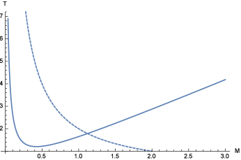
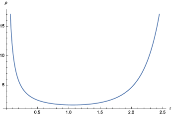
Figure 1: Left: Temperature versus mass. The solid line shows the qualitative behavior of the relation (70) while the dashed line refers to the conventional temperature of the Schwarzschild black hole. Right: The density of the matter distribution versus $r$. The figures are plotted for $\lambda=0.1$ and $M=1$.

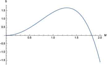
Figure 2: The entropy versus mass. The figure is plotted for $\lambda=0.1$ and $M=1$.

5 Geodesics of the polymerized metric

In this section we are going to study how light and particles will move in the geometrical background given by metric (62). This is important because from the classical trajectories of light or falling particles we understand that the corresponding space-time behaves really like a black hole. First, consider the radial null geodesics defined by $ds=0$ and $d\vartheta=d\varphi=0$. Therefore, we have

$$-a(r)dt^{2}+a^{-1}(r)dr^{2}=0\Rightarrow dt=\pm\frac{dr}{a(r)}.$$ (72)

In order to get an analytical solution we use the approximate $a(r)\sim 1-\frac{2M}{r}+M\lambda^{2}r$, for which we obtain

$$t-t_{0}=\pm\frac{\frac{2|\tanh^{-1}\left(\frac{2Mr\lambda^{2}+1}{\sqrt{8M^{2}\lambda^{2}+1}}\right)|}{\sqrt{8\lambda^{2}M^{2}+1}}+\log|Mr^{2}\lambda^{2}-2M+r|}{2\lambda^{2}M}.$$ (73)

For $r>r_{H}$, the above expression with positive (negative) sign shows that $r$ increases (decreases) as $t$ increases and thus the corresponding curve is an outgoing (incoming) radial null geodesics. For $r<r_{H}$, the situation is reversed, i.e., the positive and negative signs correspond to the incoming and outgoing curves respectively, see figure 3. A glance at this figure makes it clear that none of the null geodesics can pass through the horizon which shows the black hole nature of the underlying space-time. It is clear that in comparison with region $r>r_{H}$ the local light cones tip over in region $r<r_{H}$. This is because that while the coordinates $r$ and $t$ are space-like and time-like respectively in region $r>r_{H}$, in region $r<r_{H}$ they reverse their character. The orientation of the light cones inside the horizon shows that nothing can stay at rest in this region but will be forced to move towards the black hole center.

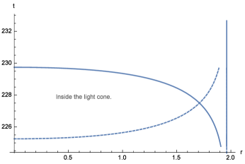
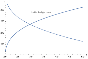
Figure 3: Left: The outgoing (dashed line) and incoming (solid line) geodesics for $r<r_{H}$. Right: The outgoing (solid line) and incoming (dashed line) geodesics $r>r_{H}$. The figures are plotted for $\lambda=0.1$ and $M=1$.

To complete our geodesics analysis, let us now consider the radial trajectory of a falling free particle. It moves along the time-like geodesics which results the following equations of motion [18]

$$a(r)\dot{t}=k,$$ (74)

$$a(r)\dot{t}^{2}-a^{-1}(r)\dot{r}^{2}=1,$$ (75)

where a dot denotes differentiation with respect to the proper time $\tau$ and $k$ is a constant that depends on the initial conditions. If we assume that the particle begins to fall with zero initial velocity from a distance $r_{0}$ for which $a(r_{0})=1$, then $k=1$. Also, for the motion around this region we have $\dot{t}\simeq 1\Rightarrow t\simeq\tau$. Therefore, we may analysis the path of the particle in view a co-moving observer which uses the proper time. Then, equations (74) and (75) give

$$\frac{d\tau}{dr}=-\left(\frac{r}{2M-M\lambda^{2}r^{2}}\right)^{1/2},$$ (76)

in which we have used the same previous approximation for $a(r)$. Upon integration we get

$$\tau-\tau_{0}=-\frac{1}{3}r\sqrt{4-2\lambda^{2}r^{2}}\,_{2}F_{1}\left(\frac{1}{2},\frac{3}{4};\frac{7}{4};\frac{r^{2}\lambda^{2}}{2}\right)\sqrt{\frac{r}{2M-\lambda^{2}Mr^{2}}},$$ (77)

where $\tau_{0}$ is an integration constant and $\,{}_{2}F_{1}\left(a,b;c;z\right)$ is a Hypergeometric function. The above equation shows that in view of the proper observer no singular behavior occurs at the horizon radius and the particle falls to the center of the black hole, see figure 4. If instead one describes the motion in terms of the coordinate time $t$, the situation becomes like the null geodesics, i.e., in view of a distance observer the particle can not pass through the horizon and it takes infinite time for the falling particle to reach the horizon, so that the $r_{H}$ is approached but never passed. All of these results show that in terms of light and particles motion the space-time given by the metric (62) behaves like a black hole as its Schwarzschild counterpart.

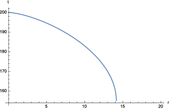
Figure 4: The trajectory of an infalling particle in terms of the proper time $\tau$. The particle falls continuously to the singularity $r=0$ in a finite proper time. The figure is plotted for $\lambda=0.1$ and $M=1$.

6 Summary

In this paper we have studied the classical polymerization procedure applied on the Schwarzschild metric. This procedure is based on a classical transformation under which the momenta are transformed like their polymer quantum mechanical counter part. After a brief review of the polymer representation of quantum mechanics, we have introduced the classical polymerization by means of which the Hamiltonian of the theory under consideration gets modification in such a way that a parameter $\lambda$, coming from polymer quantization, plays the role of a deformation parameter. In order to apply this mechanism on the Schwarzschild black hole, we first presented a Hamiltonian function for a general spherically symmetric space-time and showed that the resulting Hamiltonian equations yield the conventional Schwarzschild metric. Then, we have applied the polymerization on this minisuperspace model and solved the Hamiltonian equations once again to achieve the polymer corrected Schwarzschild metric. We saw that while the usual Schwarzschild metric is a vacuum spherical symmetric solution of the Einstein equations, this is not the case for its polymerized version obtained by the above mentioned method. Interestingly, the energy-momentum tensor of the matter field corresponding to the polymerized metric has anisotropic negative pressure sector with a dark energy-like equation of state. As expected, the unusual behavior of such a matter field resulted an uncommon behavior for the thermodynamical quantities like temperature and entropy in comparison with the traditional Schwarzschild solution. Finally, to clarify that the polymerized metric has also the black hole nature, we have investigated the null geodesics and verified that the outgoing and incoming geodesics curves can never pass through the horizon. Also, we proved that in view of a co-moving observer which uses the proper time, an infalling particle continuously falls to the center $r=0$, without experiencing something passing through the horizon. All these indicate that the underlying space-time in which the light and particles are traveling is really a black hole.

Acknowledgments: This work has been supported financially by Research Institute for Astronomy and Astrophysics of Maragha (RIAAM) under research project NO. 1/5237-107.

References

- [1] B.S. DeWitt, Phys. Rev. 160 (1967) 1113
- [2] C. Rovelli and L. Smolin, Nucl. Phys. B 442 (1995) 593
- [3] A. Ashtekar and J. Lewandowski, Class. Quantum Grav. 14 (1997) A55
- [4] C. Rovelli, Living Rev. Rel. 1 (1998) 1
-
[5]
A. Kempf, G. Mangano and R.B. Mann, Phys. Rev.
D 52 (1995) 1108 (arXiv: hep-th/9412167)
S. Hossenfelder, Living Rev. Rel. 16 (2013) 2 (arXiv: 1203.6191 [gr-qc]) -
[6]
A. Kempf, Quantum Field Theory with Nonzero Minimal
Uncertainties in Positions and Momenta (arXiv: hep-th/9405067)
A. Kempf and G. Mangano, Phys. Rev. D 55 (1997) 7909 (arXiv: hep-th/9612084)
S. Hossenfelder, Phys. Rev. D 73 (2006) 105013 (arXiv: hep-th/0603032) -
[7]
J. B. Achour and S. Brahma, Phys. Rev. D 97 (2018) 126003 (arXiv: 1712.03677
[gr-qc])
M. Bojowald, S. Brahma and D.-H. Yeom, Phys. Rev. D 98 (2018) 046015 (arXiv: 1803.01119 [gr-qc]) -
[8]
P. Nicolini, A. Smailagic and E. Spallucci,
Phys. Lett. B 632 (2006) 547 (arXiv: gr-qc/0510112)
E. Spallucci, A. Smailagic and P. Nicolini, Phys. Rev. D 73 (2006) 084004 (arXiv: hep-th/0604094) - [9] A. Corichi, T. Vukašinac and J.A. Zapata, Phys. Rev. D 76 (2007) 044016 (arXiv: 0704.0007 [gr-qc])
- [10] A. Ashtekar, S. Fairhurst and J. Willis, Class. Quantum Grav. 20 (2003) 1031 (arXiv: gr-qc/0207106)
-
[11]
G. De Risi, R. Maartens and P. Singh,
Phys. Rev. D 76 (2007) 103531 (arXiv: 0706.3586
[hep-th])
V. Taveras, Phys. Rev. D 78, (2008) 064072 (arXiv: 0807.3325 [gr-qc])
G.M. Hossain, V. Husain and S.S. Seahra, Phys. Rev. D 81 (2010) 024005 (arXiv: 0906.2798 [astro-ph])
A. Corichi and A. Karami, Phys. Rev. D 84 (2011) 044003 (arXiv: 1105.3724 [gr-qc])
S. M. Hassan and V. Husain, Class. Quantum Grav. 34 (2017) 084003 (arXiv:1705.00398 [gr-qc])
B. Vakili, K. Nozari, V. Hosseinzadeh and M. A. Gorji, Mod. Phys. Lett. A 29 (2014) 1450169 (arXiv:1408.4535 [gr-qc])
J. B. Achour, F. Lamy, H. Liu and K. Noui, Europhys. Lett. 123 (2018) 20006 (arXiv: 1803.01152 [gr-qc]) -
[12]
C.G. Boehmer and K. Vandersloot, Phys. Rev. D
76 (2007) 104030 (arXiv: 0709.2129 [gr-qc])
A. Peltola and G. Kunstatter, Phys. Rev. D 80 (2009) 044031 (arXiv: 0902.1746 [gr-qc])
E. Bianchi, Class. Quantum Grav. 28 (2011) 114006 (arXiv: 1011.5628 [gr-qc])
E.R. Livine and D.R. Terno, Class. Quantum Grav. 29 (2012) 224012 (arXiv: 1205.5733 [gr-qc])
G. Chacón-Acosta, E. Manrique, L. Dagdug and H. A. Morales-Técotl, SIGMA 7 (2011) 110 (arXiv: 1109.0803 [gr-qc])
G.M. Hossain, V. Husain and S.S. Seahra, Class. Quantum Grav. 27 (2010) 165013
M. A. Gorji, Kourosh Nozari and B. Vakili, Phys. Lett. B 735 (2014) 62 (arXiv:1312.6835 [gr-qc])
M. A. Gorji, K. Nozari and B. Vakili, Phys. Rev. D 90 (2014) 044051 (arXiv:1408.1725 [gr-qc])
M. A. Gorji, K. Nozari and B. Vakili, Class. Quantum Grav. 32 (2015) 155007 (arXiv:1506.03375 [gr-qc]) - [13] A. Corichi and T. Vukašinac, Phys. Rev. D 86 (2012) 064019 (arXiv: 1202.1846 [gr-qc])
- [14] K. Nozari, M. A. Gorji, V. Hosseinzadeh and B. Vakili, Class. Quantum Grav. 33 (2016) 025009 (arXiv: 1405.4083 [gr-qc])
-
[15]
M. Cavaglia, V. de Alfaro and A.T. Filippov, Int.
J. Mod. Phys. D 4 (1995) 661 (arXiv: gr-qc/9411070)
M. Cavaglia, V. de Alfaro and A.T. Filippov, Int. J. Mod. Phys. D 5 (1996) 227 (arXiv: gr-qc/9508062) - [16] B. Vakili, Int. J. Theor. Phys. 51 (2012) 133 (arXiv: 1102.1682 [gr-qc])
- [17] P. Kraus and F. Wilczek, A Simple Stationary Line Element for the Schwarzschild Geometry, and Some Applications, Report No.: PUPT 1474, IASSNS-HEP 94/46 (arXive: gr-qc/9406042)
- [18] R. d’Inverno, Introducing Einstein’s Relativity, Oxford University Press, New York, 1998
-
[19]
A. Corichi and P. Singh, Class. Quantum Grav. 33 (2016)
055006 (arXiv: 1506.08015 [gr-qc])
J. Olmedo, S. Saini and P. Singh, Class. Quantum Grav. 34 (2017) 225011 (arXiv: 1707.07333 [gr-qc]) - [20] H. Balasin and H. Nachbagauer, Class. Quantum Grav. 10 (1993) 2271
- [21] P. Nicolini, Int. J. Mod. Phys. A 24 (2009) 1229 (arXiv: 0807.1939 [hep-th])
- [22] Ø. Grøn and S. Hervik, Einstein’s General Theory of Relativity: With Modern Applications in Cosmology, Springer-Verlag, New York, 2007