IMEX based Multi-Scale Time Advancement in ODTLES

Abstract

[Abstract]

In this paper we overcome a key problem in an otherwise highly potential approach to study turbulent flows, ODTLES (One-Dimensional Turbulence Large Eddy Simulation). From a methodological point of view, ODTLES is an approach in between Direct Numerical Simulations (DNS) and averaged/filtered approaches like RANS (Reynolds Averaged Navier-Stokes) or LES (Large Eddy Simulations). In ODTLES, a set of 1D ODT models is embedded in a coarse grained 3D LES. On the ODT scale, the turbulent advection is modeled as a sequence of stochastic eddy events, also known as triplet maps, while the other (deterministic) terms are fully resolved in space (along the ODT-line) and time. Schmidt et al. first (2008) introduced ODTLES and Gonzalez et al. (2011) applied the model for a variety of wall-bounded flow problems. Although the results were notable for a first proof of concept, the numerical methods used are subject to debate. First of all, an unstable discretization for the large scale 3D advective terms was used as shown by Glawe (2013). The scheme can be stabilized by reducing the CFL number for the explicitly discretized LES terms to the order of the small scale ODT time step, but this of course reduces the advantage of the ODTLES multi-scale approach. The stochastic ODT eddies were also allowed to overlap two LES cells introducing an artificial smoothing (stabilizing) effect. Glawe (2013) limited the overlap consistently to one LES cell and used a stable Runge Kutta (RK) discretization, however maintaining the low CFL number problem. In this paper we adapt a new implicit/explicit (IMEX) time scheme to ODTLES in order to remedy the small CFL number issue. For the problems investigated, the results indicate a performance increase of the IMEX scheme by a factor of 17 based on the ratio of applied CFL numbers. This allowed simulations of a turbulent channel flow with characteristic friction Reynolds number $Re_{\tau}=2040$ on one Banana Pi single board computer. We compare results to available DNS data and discuss in general the efficiency and potential of ODTLES for high Reynolds number flows.

1 Introduction

The understanding of turbulence remains a relevant issue for various scientific disciplines. Direct Numerical Simulations (DNS) resolve all turbulent scales, therefore they do neither have to deal with modeling nor numerical errors while investigating physical phenomena. DNS have been, however, limited so far to moderate Reynolds numbers flows (e.g., $Re_{\tau}=5200$ in a channel flow, as shown by [Moser:2014]). In DNS the computationally feasible Re numbers are orders of magnitude below many realistic flows. This results in the use of the Reynolds Averaged Navier-Stokes (RANS) approach for industrial applications. RANS equations are obtained by applying an ensemble filter to the Navier-Stokes equations. Thus everything below the integral scale is modeled. Nowadays, Large Eddy Simulations (LES) have started to find a niche for some industrial applications. In LES, spatially filtered equations are numerically solved while the unresolved scales are modeled, mostly by eddy viscosity approaches (e.g., see [drikakis2006turbulent] and references within).

For canonical highly turbulent flows, LES still needs to resolve a wide range of scales including at least some portion of the inertial range of the turbulent cascade. This limits the achievable Reynolds numbers in comparison to the RANS simulations. The parameterization of small scales in RANS and LES is especially problematic for multi-physics regimes such as buoyant and reacting flows, because much of the complexity present in these phenomena is inherent to the unresolved scales. Alternative model approaches have been proposed to overcome these issues. The One-Dimensional Turbulence (ODT) model introduced by Kerstein (see [AR-Kerstein1999, AR-Kerstein2001]) reduces the dimensionality of the problem instead of filtering/modeling small scales. The 3D turbulence is described within a 1D sub-domain which includes the full turbulent cascade, whereby the numerical representation of molecular diffusive effects becomes computationally feasible. Meiselbach [Meiselbach2015] described wall-bounded flows with $Re_{\tau}=6\,\cdot 10^{5}$ using an adaptive ODT version [Lignell2012]. This is clearly in the range of real world applications, which shows the efficiency of ODT for the simulation of large Re number flows. Nonetheless, ODT is limited to applications that have a reasonable symmetry in a statistical sense, i.e. the underlying studied phenomena must be predominantly one dimensional. Considering these assumptions, the variety of flows where the model developed by Kerstein has been applied [AR-Kerstein2001, WT-Ashurst2005, Lignell2012, Meiselbach2015, Jozefiketal:2015, FragnerSchmidt:2017, Medinaetal:2018] is remarkable.

To benefit from the efficiency of 1-D approaches similar to ODT in more complex flow scenarios, several approaches have combined these 1D models with 3D LES. We reference LES-ODT [Cao:2008], LES-LEM [Menon:2011], LEM3D [Sannan:2013], and ODTLES [RC-Schmidt2010, ED-Gonzalez-Juez2011, Glawe2013, GlaweThesis2015] as examples. In fully resolved DNS, a computational effort proportional to $N_{DNS}^{3}$ is expected, with $N_{DNS}$ being the total number of cells per resolved direction (assuming an equidistant grid). As a comparison, ODTLES expects a computational effort proportional to $3N_{LES}^{2}N_{ODT}$ [ED-Gonzalez-Juez2011], whereby $N_{LES}$ and $N_{ODT}$ are the number of cells in the coarse LES grid and in the finely resolved 1-D subdomain, respectively. This is a significant computational improvement and therefore makes ODTLES a model worth of studying. To include a simple approximation of an explicit time step size leads to $N_{DNS}^{4}$ and $3N_{LES}^{2}N_{ODT}^{2}$ in previous ODTLES implementations while the IMEX-ODTLES approach introduced in this work scales with $3N_{LES}^{3}N_{ODT}$.

In this work we introduce a stable and second-order accurate ODTLES time advancement using Implicit-Explicit (IMEX) Runge-Kutta time schemes. These time schemes exploit the large time steps considering the extreme spatial scale gap between the LES-coarse 3D resolution and the 1D Kolmogorov scales resolved for ODT in ODTLES. The paper is structured as follows. In Section 2, a brief overview of the already established concept of ODT is made. Section 3 illustrates the multi-dimensional extension of ODT, ODTLES, with a description of the governing equations of the model in Section 3.1. Section 4 summarizes the time discretization schemes applicable to ODTLES. The current time advancement scheme applied so far in ODTLES is briefly explained in Section 4.1. Section 4.2 introduces a novel ODTLES time scheme based on recent Implicit-Explicit Runge-Kutta (IMEX) schemes. To illustrate the ODTLES model capabilities, turbulent channel flows up to a friction Reynolds number $Re_{\tau}=2040$ are studied in Section 5. Calculations were performed using one Banana Pi M64 single-board-computer only. Finally, a summary and some concluding remarks are given in Section 6.

2 One-Dimensional Turbulence Model (ODT)

We begin the discussion of the ODT model by referencing the Navier-Stokes governing equations for incompressible flow, noted here for a velocity component $u_{i}$ in $x_{i}$-direction, $i\in\{1,2,3\}$:

$$\frac{\partial u_{i}}{\partial t}+\frac{1}{\rho}\frac{\partial p}{\partial x_{i}}+\sum_{j=1}^{3}\frac{\partial}{\partial x_{j}}u_{j}\cdot u_{i}=\nu\sum_{j=1}^{3}\frac{\partial^{2}}{\partial x_{j}^{2}}u_{i}+F_{i}.$$ (1)

Here $p$ denotes the pressure and $F_{i}$ the external forces acting on the flow. The kinematic viscosity $\nu$ and the density $\rho$, for simplicity, are assumed constant. We note that, throughout this work, the use of indexes does not imply the traditional Einstein summation, and therefore, all summations across indexes must be explicitly written.

Mass and energy conservation are given by the divergence condition of the velocity field,

$$\sum_{j=1}^{3}\frac{\partial}{\partial x_{j}}u_{j}=0.$$ (2)

ODT simulates 3D turbulent behavior within a 1D subdomain (ODT line) using a stochastic processes to model the effects induced by the non-linear advective term. The most recent, yet standard ODT formulation for incompressible flow, which we will refer in this paper as the standalone ODT formulation, treats the three velocity components as scalar profiles in the line. The three components of the velocity fulfill net kinetic energy conservation in the ODT line.

In order to apply ODT as a closure model in ODTLES, the standalone ODT implementation needs to be modified: the traditional notion of a line in ODT, is replaced by a stack configuration which is finely discretized in the line direction, as in [RC-Schmidt2010]. Instead of three velocity components, only two velocity components are defined in the line and evolved by means of a transport equation. The velocity pointing in the ODT line direction is not considered to evolve according to a transport equation, rather, it is given by the incompressibility condition. Figure 1 illustrates the notion of the ODT line in the ODTLES context. It will become clear later, that the stack dimensions in $i,j$ (orthogonal directions to the line) correspond to the LES cell sizes in the $i,j$ directions.

Figure 1: ODT line representation, or stack, showing the $u_{i}$ and $u_{j}$ velocity components defined in the line. $u_{k}$ is not considered to evolve based on a transport equation in the line.

For an ODT line pointing into $x_{k}$-direction, $k\in\{1,2,3\}$, we can write the ODT governing equation for incompressible flow as:

$$\frac{\partial u_{i}}{\partial t}+\mathit{eddy}_{k,i}(u_{j},x_{0},l)=\nu\frac{\partial^{2}}{\partial x_{k}^{2}}u_{i}+F_{i}\;\text{for}\;i,j\in\{1,2,3\}\setminus k.$$ (3)

The reader should note that we have intentionally introduced a second index $k$, which refers to the ODT line direction. In Eq. (3), $l$ is the eddy size and $x_{0}$ is the left edge of the eddy (or its starting location, without loss of generality). Also, there should be no confusion regarding Eq. (3): This equation only represents the evolution in the standalone ODT formulation for incompressible flow with no mean advection effect in the line. The instantaneous eddy function in Eq. (3) is defined as the following transformation [AR-Kerstein2001],

$$\mathit{eddy}_{k,i}:u_{i}(x_{k},t)\rightarrow{u_{i}}[f(x_{k},x_{0},l),t]+{c}_{i}(u_{j})K(x_{k})\;\text{for}\;i,j\in\{1,2,3\}\setminus k.$$ (4)

The triplet map definition $x_{k}\to f(x_{k},x_{0},l)$ (illustrated in Fig. 2), is given by [AR-Kerstein1999]

$$f(x_{k},x_{0},l)=x_{0}+\begin{cases}3(x_{k}-x_{0}),&\mathrm{if}\;\;x_{0}\leq x_{k}\leq x_{0}+\frac{1}{3}l\\ 2l-3(x_{k}-x_{0}),&\mathrm{if}\;\;x_{0}+\frac{1}{3}l\leq x_{k}\leq x_{0}+\frac{2}{3}l\\ 3(x_{k}-x_{0})-2l,&\mathrm{if}\;\;x_{0}+\frac{2}{3}l\leq x_{k}\leq x_{0}+l\\ (x_{k}-x_{0}),&\mathrm{else}.\end{cases}$$ (5)

Likewise, the Kernel function $K(x_{k})$ in Eq. (4), is given by

$$K(x_{k},x_{0},l)=x_{k}-f(x_{k},x_{0},l).$$ (6)

In combination with the amplitudes $c_{i}$, $K(x_{k})$ assures momentum and energy conservation and controls the energy redistribution among the velocity components.

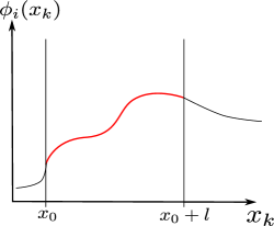
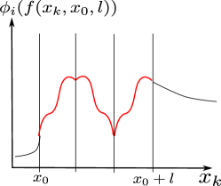
(a) Profile before triplet map.	(b) Profile after triplet map.

Figure 2: Illustration of a continuous triplet map in Eq. (5): The profile within the eddy range $x_{0}<x_{k}<x_{0}+l$ is replaced by $3$ compressed copies of the original profile, while the middle copy is reversed.

Determination of the amplitudes $c_{i}$ requires additional modeling. Kerstein et al [AR-Kerstein2001] derive them as

$$c_{i}=\frac{27}{4l}\left(-u_{K;k,i}+\textrm{sgn}(u_{K;k,i})\sqrt{u_{K;k,i}^{2}+\sum_{j\neq k}\frac{1}{2}T_{ij}u_{K;k,j}^{2}}\right)\,;\,i\neq k,$$ (7)

where sgn is the sign function. The definition

$$u_{K;k,i}\equiv\frac{1}{l^{2}}\int u_{k,i}[f(x_{k},x_{0},l)]K(x_{k},x_{0},l){\rm\,d}x_{k},$$ (8)

is also used, as well as the transfer matrix [GlaweThesis2015],

$$\frac{1}{2}T=\frac{1}{2}\begin{pmatrix}-1&1\\ 1&-1\\ \end{pmatrix}.$$ (9)

The prefactor $\frac{1}{2}$ in Eq. (7) and (9) is chosen based on the reasoning of the equalization of available energies for the two available velocity components $u_{k,i}$, $u_{k,j}$ [ED-Gonzalez-Juez2011, GlaweThesis2015]. Note that the velocity component $u_{i}$ is only changed by the eddy function within the eddy range $[x_{0},l]$. The energy redistribution in ODT is a model for the pressure-fluctuation effect in a 3D flow and is therefore called pressure scrambling [AR-Kerstein2001].

Time-advancement of Eq. (3) takes place in an intermittent way. As it is well described in all of the ODT implementations so far (see, e.g. [WT-Ashurst2005]), eddy events (or eddy trials in this case) are tested on a forecasting approach based on the current state of the flow and a sampled eddy size $l$ and position $x_{0}$. If an eddy event is accepted and deemed to be implemented, the diffusive (and forcing) terms of Eq. (3) are advanced in time up to the instant where the eddy event trial took place (this is normally called a catchup-diffusion event in ODT). The reader is suggested to consult the work by Ashurst and Kerstein [WT-Ashurst2005] or Lignell [Lignell2017] in order to dive into the details of eddy event selection and implementation in ODT.

3 ODTLES Model and Discretization

Similar to Very Large Eddy Simulations (VLES), in ODTLES the 3D governing equations are resolved on a relatively coarse grid, e.g. Figure 3(a). As it was commented before, the ODT turbulent advancement is embedded in 1D LES stacks (see Figure 1). The line allows the suitable resolution for scales of motion starting at the smallest LES cell size and finishing at the Kolmogorov scales. To create an orientation independent approach, the three Cartesian directions are highly resolved in three separate grids as illustrated in Figures 3(b-d).

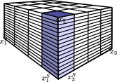
(a) LES grid, containing LES	(b) Grid 1, containing	(c) Grid 2, containing	(d) Grid 3, containing
variables $U_{i}$ and $P$.	variables $u_{1,i}$.	variables $u_{2,i}$.	variables $u_{3,i}$.

Figure 3: In ODTLES the velocities are resolved using multiple grids, as in (b-d). 3D-coarsened properties, corresponding to a standard LES grid are for illustration represented with $N_{\rm LES}=4$ cells per direction in (a). The discrete highly resolved properties are represented for illustration by $N_{\rm ODT}=16$ cells in (b-d).

We now formally harmonize the notation in this study with the velocity and pressure variables notation used in the work by Gonzalez-Juez et al [ED-Gonzalez-Juez2011]. On one hand, as it may have been already visualized by the reader, velocity components $u_{k,i}$ corresponding to Grid $k$ (in Figures 3(b-d)) are highly resolved in $x_{k}$-direction. On the other hand, coarsely resolved pressure and velocity variables in the LES grid (Figure 3(a)) are denoted as $P$ and $U_{i}$, respectively.

The turbulent ODT advancement in ODTLES takes place in the corresponding highly resolved direction. In Figure 3(c), one ODT line is highlighted. ODT eddies implemented result then in a 3D turbulent net transport in $x_{2}$-direction. Additionally, diffusive transport in this direction is finely resolved, which may allow inclusion of sub-Kolmogorov scales, e.g. in case of high Schmidt numbers.

The numerical difference operators in $X_{j}$-direction represented in the coarsely resolved grid are denoted as $\frac{\delta}{\delta X_{j}}$ and $\frac{\delta^{2}}{\delta X_{j}^{2}}$. Similarly, the finely resolved difference operators in $x_{j}$-direction are $\frac{\partial}{\partial x_{j}}$ and$\frac{\partial^{2}}{\partial x_{j}^{2}}$. The current ODTLES implementation is discretized using staggered grids with face-centered velocity components $u_{k,i}$ and $U_{i}$, as well as a cell-centered coarse grained pressure field $P$. Diffusive and advective terms are spatially approximated with second order central schemes.

To derive a reasonable ODTLES interpretation of the governing equations, some operators connecting the different numerical grids are required. The 1D upscale operator $[l_{k}]$ creates a coarsely resolved velocity variable from the highly resolved velocity in $x_{k}$-direction,

$$U_{k,i}=[l_{k}]u_{k,i}=\frac{1}{\Delta X_{k}}\int_{-\frac{\Delta X_{k}}{2}}^{\frac{\Delta X_{k}}{2}}u_{k,i}{\rm\,d}x_{k}^{\prime}.$$ (10)

The consistency condition,

$$U_{k,i}=U_{i},$$ (11)

has to be fulfilled by the ODTLES governing equations (see section 3.1). As the reader should note, Eq. (10) is nothing more than a spatial filter operation of the finely resolved velocity field $u_{k,i}$ over one LES cell.

The inverse of the upscaling operation is the downscaling operation

$$u_{k,i}=[l_{k}^{-1}]U_{i}.$$ (12)

Generally speaking, a field $u_{k,i}$ cannot be reconstructed exactly from its large-scale counterpart (i.e., $[l_{k}^{-1}][l_{k}]\neq\mathbbm{1}$ with unity operator $\mathbbm{1}$). However, a numerical approximation of the deconvolution of all coarsely resolved information present in $u_{k,i}$ has been introduced by Schmidt [RC-Schmidt2010] and later improved by the author in [GlaweThesis2015]. Similar reconstruction operations are performed to derive Finite Volume methods. This method is high-order accurate and avoids to create noticeable discontinuities. The integral constraint required for a consistent ODTLES model,

$$U_{i}=[l_{k}][l_{k}^{-1}]U_{i},$$ (13)

is also fulfilled by construction.

Since the grids in Figures 3(b-d) are different discrete representations of the same physical domain, Section 3.1 presents the governing equations represented by the three overlapping grids, including various coupling terms, which are not present in standard LES schemes. An interpretation of these terms can be found in [GlaweThesis2015].

3.1 ODTLES Governing Equations

The ODTLES governing equations contain velocity components discretized in three different grids with different spatial resolutions. There are coupling terms between the grids which ensure a consistent coarse grained velocity field in each of the grids (ensure Eq. (11)). It is possible to derive the ODTLES system of equations, including these coupling terms from the incompressible Navier-Stokes equations. Since this has already been done elsewhere in another study from the author [GlaweThesis2015], we do not include the derivation in this work.

As it was done in [RC-Schmidt2010, ED-Gonzalez-Juez2011, Glawe2013, GlaweThesis2015], only two velocity components are advanced in each of the ODTLES grids. The third component, $u_{k,k}$, defined in the highly resolved $x_{k}$-direction, is computed by means of the incompressibility condition. The divergence free velocity field can only be determined after solving the mass conservation equation. We refer to this divergence-free field in this section by means of the symbols, $\widehat{u}_{k,i}$ and $\widehat{U}_{i}$, for the finely resolved and coarsely resolved (LES grid) velocity fields, respectively. As shown in [GlaweThesis2015], it is not necessary to enforce the divergence condition on the finely-resolved fields. Given that the finely resolved velocities $u_{k,i},u_{k,j}$ fulfill conservation of mass and kinetic energy (zero-divergence) in standalone ODT, $u_{k,k}$ is the only component that needs to be determined. The only necessary condition for complete zero-divergence in the coarse and fine spatial scale is then the zero-divergence of the coarsely resolved field,

$$\sum_{j=1}^{3}\frac{\delta}{\delta X_{j}}\widehat{U}_{j}=0.$$ (14)

The divergence-free coarse grained velocity field in Eq. (14) is enforced by solving a modified Poisson equation for the LES pressure [ED-Gonzalez-Juez2011].

$$\frac{\partial}{\partial t}\sum_{j=1}^{3}\frac{\delta}{\delta X_{j}}U_{j}=-\frac{1}{\rho}\frac{\delta^{2}P}{\delta X_{i}^{2}}.$$ (15)

The LES pressure $P$ has then the only purpose of correcting a non-zero-divergence velocity field into a divergence-free velocity field over an LES time-range $\delta T$.

Momentum conservation for a finely resolved velocity component $u_{k,i}$, considering the LES pressure gradient, mean advection, turbulent advection and diffusion effects in ODTLES is then given by

$$0 = \frac{\partial u_{k,i}}{\partial t}+\frac{1}{\rho}\frac{\delta P}{\delta X_{i}}$$ (16)

$$+\frac{\partial}{\partial x_{k}}\widehat{u}_{k,k}\cdot u_{k,i}+\frac{\delta}{\delta X_{i}}\widehat{u}_{k,i}\cdot u_{k,i}+\frac{\delta}{\delta X_{j}}\widehat{u}_{k,j}\cdot u_{k,i}+\mathbb{C}^{LES}_{j\rightarrow k,i}$$

$$+\left(\mathit{eddy}_{k,i}-\nu\frac{\partial^{2}}{\partial x_{k}^{2}}u_{k,i}-F_{i}\right)-\nu\frac{\delta^{2}}{\delta X_{i}^{2}}u_{k,i}+\mathbb{C}^{ODT}_{j\rightarrow k,i}.$$

In Eq. (16), $\{i,j,k\}$ are positive permutations of $\{1,2,3\}$ with $i\neq k$. The turbulent ODT advancement $\mathit{eddy}_{k,i}$ is the same one defined in section 2. The coupling terms $\mathbb{C}^{ODT}_{j\rightarrow k,i}$ and $\mathbb{C}^{LES}_{j\rightarrow k,i}$, as well as the nature of the additional diffusive term $\nu\frac{\partial^{2}}{\partial X_{i}^{2}}u_{k,i}$ are investigated in section 3.2.

3.2 ODTLES Grid Coupling

The ODT advancement within a specific ODT line in $x_{k}$-direction, or conversely, of all the ODT lines in ODTLES grid $k$, influences the coarse grained velocity fields. This information is coupled between ODTLES grids (from grid $k$ to grids $i,j$) to guarantee that the coarse grained velocity fields across grids are consistent ($U_{k,i}=U_{j,i}$). All highly resolved ODTLES terms in one grid, i.e. highly resolved advection, ODT turbulent advection and diffusion, are communicated to the other ODTLES grids.

The coupling term corresponding to the standalone ODT advancement for velocity component $i$ within ODTLES, from grid $j$ to grid $k$, can be written as

$$\mathbb{C}^{ODT}_{j\rightarrow k,i}=[l_{k}^{-1}][l_{j}]\left(\mathit{eddy}_{j,i}-\nu\frac{\partial^{2}}{\partial x_{j}^{2}}u_{j,i}\right).$$ (17)

The term in brackets in Eq. (17) includes the ODT terms in Eq. (3).The forcing $F_{i}$ in Eq. (3) is considered a constant and can therefore be easily subtracted from the time advancement in order to calculate the coupling term $\mathbb{C}^{ODT}_{j\rightarrow k,i}$. The upscaling (in grid $j$) and subsequent downscaling (to grid $k$) operations lead to the flux communication from grid $j$ to grid $k$.

In previous studies [ED-Gonzalez-Juez2011], Eq. (16) exhibited an additional term $\nu\frac{\delta}{\delta X_{j}}\left(\frac{\partial}{\partial x_{j}}u_{j,i}\right)$. This term is indirectly resolved by the standalone ODT advancement in ODTLES due to the coupling from grid $j$ to grid $k$ of $\nu[l_{k}^{-1}][l_{j}]\frac{\partial^{2}}{\partial x_{j}^{2}}u_{j,i}$ [GlaweThesis2015]. On the other hand, the diffusive term $\nu\frac{\partial^{2}}{\partial X_{i}^{2}}u_{k,i}$, still appearing in Eq. (16), is coarsely resolved and therefore added to the equation given that there is no ODT line where the velocity component $u_{i}$ can be highly resolved in $x_{i}$-direction.

There is another LES coupling term, which includes all fluxes in the highly resolved advection not included in the coarse grained advective fluxes. This coupling term can be written as

$$\mathbb{C}^{LES}_{j\rightarrow k,i} = [l_{k}^{-1}][l_{j}]\left(\frac{\delta}{\delta X_{i}}\widehat{u}_{j,i}\cdot u_{j,i}-\frac{\delta}{\delta X_{i}}\widehat{U}_{j,i}\cdot U_{j,i}\right)$$ (18)

$$+ [l_{k}^{-1}][l_{j}]\left(\frac{\partial}{\partial x_{j}}\widehat{u}_{j,j}\cdot u_{j,i}-\frac{\delta}{\delta X_{j}}\widehat{U}_{j,j}\cdot U_{j,i}\right)$$

$$+ [l_{k}^{-1}][l_{j}]\left(\frac{\delta}{\delta X_{k}}\widehat{u}_{j,k}\cdot u_{j,i}-\frac{\delta}{\delta X_{k}}\widehat{U}_{j,k}\cdot U_{j,i}\right).$$

The following definitions were used for the non-zero-divergence and divergence-free velocity fields, respectively,

$$U_{j,i}=[l_{j}]u_{j,i}\;\;\text{and}\;\;\widehat{U}_{j,i}=[l_{j}]\widehat{u}_{j,i}.$$ (19)

Note that the terms in Eq. (18) correspond to individual Reynolds Stress terms which are modeled in standard LES schemes, but are numerically fully resolved in ODTLES. Therefore, using ODTLES without ODT turbulent advection shows beneficial properties for low Reynolds number wall-bounded flows. This unclosed ODTLES model is called unclosed extended LES (U-XLES), and was introduced by the author in [GlaweThesis2015].

Both $\mathbb{C}^{ODT}_{j\rightarrow k,i}$ and $\mathbb{C}^{LES}_{j\rightarrow k,i}$ coupling terms are required to ensure matching (consistent) large scale fields in all highly resolved grids, as demanded by Eq. (11). A more detailed proof that the introduced coupling terms lead to consistent large scale fields can be found in [GlaweThesis2015].

4 Time Integration

4.1 CN-RK3 Time Integration

The first versions of ODTLES advanced Eq. (16) in a one-step fashion, using an explicit Euler numerical method (parallel to the standalone ODT eddy trial and implementation procedure) [RC-Schmidt2010, ED-Gonzalez-Juez2011]. This implementation was proven to be unstable [GlaweThesis2015] for reasonable large time steps.

It is possible to advance the momentum equation over a time-step size $\Delta t$, from $t$ to $t+\Delta t$, by means of a temporal operator-splitting within a predictor-corrector scheme. This leads to the numerical scheme stated in Table 1, first introduced by the author in a previous work [GlaweThesis2015]. The advection terms are advanced using a standard second-order Crank-Nicolson scheme in the highly resolved direction and a 3-stage third-order TVD Runge-Kutta scheme by Spiteri and Ruuth [Spiteri:2002] for the coarsely resolved direction.

The combination of the Crank-Nicolson and Runge-Kutta schemes (termed here as CN-RK3), is stable and converges for small time-step sizes, which are dependent on the finely resolved cell size. This is a modified CFL condition for ODTLES,

$$\Delta t\leq CFL\cdot\;min_{k,i}\left(\frac{\Delta x_{k}}{u_{k,i}}\right).$$ (20)

Here we consider the constant Courant-Friedrichs-Lewy (CFL) number $CFL\leq 1$.

Applying the CFL condition given by Eq. (20) leads to small time-steps in comparison to those which could be obtained by an advancement governed by the coarse-grained grid. This is the main motivation to switch to another type of schemes, as shown in section 4.2.

Table 1: The CN-RK3-ODTLES time cycle in semi-discrete notation is shown. During one predictor (p) - corrector (c) CN-RK3-ODTLES time cycle, the Explicit Euler (EE1), Runge-Kutta 3rd order (RK3), and Crank-Nicolson (CN) schemes are used for the temporal integration. The ODT advancement within ODTLES takes place in p $4$ (note the additional diffusion term in comparison to Eq. (3), commented in Section 3.2). Some implementation comments regarding this step and the coupling step are given for the IMEX scheme in B, and can be implemented here in a similar way. Step c $2$ refers to solving the Poisson equation, Eq. (15). The Algebraic Multi-Grid (AMG) solver used here is part of the hypre package distribution [Falgout02hypre:a]. Mass conservation must be enforced in the corrector step, as explained in Section 3.1. Superindexes $*$ used here refer to predictor values. Further details of the numerical implementation can be found in [GlaweThesis2015].

Substep	Advanced term	Time scheme
p $1$	$\displaystyle u_{k,i}^{n+1,*}=u_{k,i}^{n}+\Delta t\left(\frac{\delta}{\delta X_{i}}\widehat{u}_{k,i}^{n}\cdot u_{k,i}^{n}+\frac{\delta}{\delta X_{j}}\widehat{u}_{k,j}^{n}\cdot u_{k,i}^{n}\right)$	RK3
p $2$	$\displaystyle u_{k,i}^{n+1,***}=u_{k,i}^{n+1,*}+\Delta t\left(\frac{\partial}{\partial x_{k}}\widehat{u}_{k,k}^{n}\cdot u_{k,i}^{n+1,*}\right)$	CN
p $3$	$\displaystyle u_{k,i}^{n+1,***}=u_{k,i}^{n+1,**}-\Delta t\left(\mathbb{C}^{LES}_{j\rightarrow k,i}\right)$	EE1
p $4$	$\displaystyle u_{k,i}^{n+1,****}=u_{k,i}^{n+1,***}+\Delta t\left(\mathit{eddy}_{k,i}-\nu\frac{\partial^{2}}{\partial x_{k}^{2}}u_{k,i}^{n+1,***}-F_{i}-\nu\frac{\delta^{2}}{\delta X_{i}^{2}}u_{k,i}^{n+1,***}\right)$	EE1
p $5$	$\displaystyle u_{k,i}^{n+1,*****}=u_{k,i}^{n+1,****}-\Delta t\left(\mathbb{C}^{ODT}_{j\rightarrow k,i}+F_{i}+\nu\frac{\delta^{2}}{\delta X_{i}^{2}}u_{k,i}^{n+1,***}\right)$	EE1
c $1$	$\displaystyle U_{i}^{n+1,*}=U_{k,i}^{n+1,*}=[l_{k}]u_{k,i}^{n+1,*****}$	Upscaling
c $2$	$\displaystyle 0=\sum_{j=1}^{3}\frac{\partial}{\delta X_{i}}U_{i}^{n+1,*}\rightarrow\frac{\delta}{\delta X_{i}}P^{n+1}$	AMG
c $3$	$\displaystyle U_{i}^{n+1}=U_{i}^{n+1,*}-\Delta t\left(\frac{1}{\rho}\frac{\delta}{\delta X_{i}}P^{n+1}\right)$	EE1
c $4$	$\displaystyle u_{k,i}^{n+1}=[l_{k}^{-1}]U_{i}^{n+1}$	Downscaling
c $5$	$\displaystyle\widehat{u}_{k,i}^{n+1}=u_{k,i}^{n+1}$ for $i\neq k\rightarrow\widehat{u}_{k,k}$ (from mass conservation)	Divergence
		condition

The advecting velocities $\widehat{u}_{k,i}$ and $\widehat{u}_{k,j}$ in Eq. (16) (or step p $1$ in Table 1) can be calculated in two ways:

• As in Schmidt et al [RC-Schmidt2010] and Gonzalez et al [ED-Gonzalez-Juez2011], the velocities advecting any property in the non-ODT advection terms are time-averaged over all predictor steps (see table 1), and subsequently pressure corrected. The time-average, e.g. for $\widehat{u}_{k,j}$, is

  $$\widehat{u}_{k,j}(t)=\frac{1}{\Delta t}\int_{t-\Delta t}^{t}u_{k,j}{\rm\,d}t^{\prime}.$$ (21)

• The advecting velocities for the next time-step are chosen as the pressure corrected velocities of the current time step, as shown in table 1, step c $5$.

• For small time-steps such as the ones given by Eq. (20), no significant difference between the two advecting velocity treatments can be determined for turbulent wall-bounded flow results [GlaweThesis2015].

4.2 IMEX Time Integration for ODTLES

The IMEX implementation is a three-register [3R] implementation of the [2R]IMEXRKCB2 scheme described by Cavaglieri and Bewley [Cavaglieri:2015]. The scheme is modified in order to include the coupling terms and in general to be adequated to the ODTLES philosophy.

Cavaglieri and Bewley split an ordinary differential equation in two components. In our ODTLES notation, this refers to

$$\frac{d}{dt}u_{k,i}=f(u_{k,i},t)+g(u_{k,i},t).$$ (22)

The stiff part of the problem,

$$f(u_{k,i},t)=\frac{\partial}{\partial x_{k}}\widehat{u}_{k,k}\cdot u_{k,i},$$ (23)

is solved by an implicit scheme. Meanwhile, the non-stiff part,

$$g(u_{k,i},t) = \frac{\delta}{\delta X_{i}}\widehat{u}_{k,i}\cdot u_{k,i}+\frac{\delta}{\delta X_{j}}\widehat{u}_{k,j}\cdot u_{k,i}$$ (24)

$$+ \left(\mathit{eddy}_{k,i}-\nu\frac{\partial^{2}}{\partial x_{k}^{2}}u_{k,i}-F_{i}\right)-\nu\frac{\delta^{2}}{\delta X_{i}^{2}}u_{k,i},$$

is solved by an explicit scheme. The reader should note that the coupling terms and the pressure correction term are not included so far. This means that an IMEX sub-cycle is a predictor step that is then corrected with the pressure correction as usual and the XLES grid coupling. The latter is an additional operation that is not foreseen in the IMEX scheme.

Both the implicit and explicit parts of Eq. (22) in an IMEX scheme are advanced synchronously to intermediate points in time at the end of an IMEX subcycle [Cavaglieri:2015]. This is a physical intermediate time-level which gives the possibility for the application of the coupling terms and correction steps. The Poisson pressure projection can be solved in each of these synchronous instants to increase the time accuracy of large scale pressure effects.

The full ODT advancement in ODTLES is interpreted as an explicit term in Eq. (24). No time integration is performed for the advecting velocities $\widehat{u}_{k,i}$ and $\widehat{u}_{k,j}$, given that for each sub-cycle, a divergence free velocity field is available from the last sub-cycle step (see Table 3). In contrast to the CN-RK3-scheme introduced in section 4.1, the advecting velocities are treated similar to standard LES and DNS schemes in the new IMEX scheme.

Figure 4 illustrates the advective transport along a black arrow in a 2D ODTLES-like domain with a coarse grained and a highly resolved direction. As shown in Figure 4, the CN-RK3 scheme is only able to advance information in time by approximating a series of RK3 steps along the coarse grained direction and CN steps in the highly resolved direction (p $1$ and p $2$ in Table 1). Thus, a converging overall time scheme depends on the finely resolved cell size. However, the IMEX scheme predicts the explicit (in coarse direction) and implicit (in highly resolved direction) advected RHS and advances both together (p $1.1$ - $2.3$ in table 3), which allows to circumvent the limitation of the very small time-steps (see Fig. 4).

 

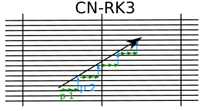
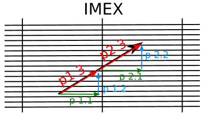
Figure 4: The two sketches illustrate the differences between the CN-RK3 and the IMEX scheme in ODTLES implementations. The information is linearly advected on a 2D grid with a very high aspect ratio along the black arrow (a 2D version of an ODTLES grid). Both in the CN-RK3 and the IMEX scheme require the advancement of coarsely resolved and finely resolved terms (horizontal and vertical components of the diagonal, respectively).

The time-step size is based on the coarse grained grid,

$$\Delta t\leq CFL\cdot\;min_{i}\left(\frac{\Delta X_{i}}{U_{i}}\right).$$ (25)

The constant CFL number is set as $CFL\leq 0.25$ based on numerical explorations. Results proving the stability of the method based on comparisons to DNS can be found in Section 5.

Based on the considerations done so far, and starting from the general three-register implementation of the IMEXRKCB2 scheme by Cavaglieri and Bewley [Cavaglieri:2015], we develop the IMEX ODTLES time advancement, as summarized in Table 3 and algorithmically explained in B. As in the general [3R]IMEXRKCB2, we use the IMEX coefficients derived in [Cavaglieri:2015], which are summarized in the Butcher tableaux (Table 2).

Due to the coupling step, the IMEX ODTLES scheme mandates the synchronization of the sub-cycles, and therefore the explicit and implicit coefficients $b_{2},b_{3}$ should match each other, i.e. $b_{2}^{IM}=b_{2}^{EX}$ and $b_{3}^{IM}=b_{3}^{EX}$ (see Table 2). The explicit and implicit terms can then be coupled across ODTLES grids at times $t+b_{2}\Delta t$ and $t+(b_{2}+b_{3})\Delta t$, respectively.

Table 2: Butcher tableaux for ODTLES IMEX coefficients. Coefficients for the implicit scheme are shown in the left table, while the coefficients for the explicit scheme are shown in the right table.

0	0
$c_{2}=2/5$	0	$a_{22}^{IM}=2/5$
$c_{3}=1$	0	$a_{32}^{IM}=5/6$	$a_{33}^{IM}=1/6$
	0	$b_{2}=5/6$	$b_{3}=1/6$

0	0
$c_{2}=2/5$	$a_{21}^{EX}=2/5$	0
$c_{3}=1$	0	$a_{32}^{EX}=1$	0
	0	$b_{2}=5/6$	$b_{3}=1/6$

Table 3: The IMEX-ODTLES scheme is divided into two sub-cycles. Each sub-cycle contains a set of predictor steps as in the [3R]IMEXRKCB2 scheme [Cavaglieri:2015] (e.g. p $1.1$ - p $1.4$), followed by a set of corrector steps involving the pressure correction (e.g. c $1.1$ - c $1.5$). Superindexes $\#$ used here indicate sub-steps within the IMEX cycle while superindexes $*$ refer to predictor values advanced in physical space. The time-steps are solved using Explicit Euler (EE1) and Implicit Euler (IE1) methods. The changes due to an IE1-step must be stored, i.e. the RHS term $R_{IM}$, as well as the explicit RHS terms, $R_{EX}$, which are calculated as usual with the information available at the current time level. The time level column reports the time after solving the corresponding step in the scheme; a square bracket notation is used in this column to indicate that the time level is relative within the IMEX sub-cycle. Details of the numerical implementation can be found in B.

Substep	Advanced term	Time level	Time scheme
p $1.1$	$\displaystyle u_{k,i}^{n+2/5,\#}=u_{k,i}^{n}+R_{EX}(u_{k,i}^{n})\;a_{21}^{EX}\Delta T$	$[t+2/5\Delta T]$	EE1
p $1.2$	$\displaystyle u_{k,i}^{n+4/5,\#}=u_{k,i}^{n+2/5,\#}+R_{IM}(u_{k,i}^{n+2/5,\#})\;a_{22}^{IM}\Delta T$	$[t+4/5\Delta T]$	IE1
p $1.3$	$\displaystyle u_{k,i}^{n+5/6,*}=u_{k,i}^{n}+\left[R_{EX}(u_{k,i}^{n})+R_{IM}(u_{k,i}^{n+2/5,\#})\right]\;b_{2}\Delta T$	$t+5/6\Delta T$	EE1
p $1.4$	$\displaystyle u_{k,i}^{n+5/6,**}=u_{k,i}^{n+5/6,*}-\left[\mathbb{C}^{LES}_{j\rightarrow k,i}+\mathbb{C}^{ODT}_{j\rightarrow k,i}+F_{i}+\nu\frac{\delta^{2}}{\delta X_{i}^{2}}u_{k,i}^{n}\right]\;b_{2}\Delta T$	$t+5/6\Delta T$	EE1
c $1.1-1.2$	$\displaystyle U_{i}^{n+5/6,*}=[l_{k}]u_{k,i}^{n+5/6,**}$ and $\displaystyle 0=\sum_{j=1}^{3}\frac{\partial}{\partial X_{i}}U_{i}^{n+5/6,*}\rightarrow\frac{\partial}{\partial X_{i}}P^{n+5/6}$	$t+5/6\Delta T$	Upscaling and
			AMG
c $1.3-1.4$	$\displaystyle U_{i}^{n+5/6}=U_{i}^{n+5/6,*}-\left[\frac{1}{\rho}\frac{\partial}{\partial X_{i}}P^{n+5/6}\right]\;b_{2}\Delta T$ and	$t+5/6\Delta T$	EE1 and
	$\displaystyle u_{i,k}^{n+5/6}=[l_{k}^{-1}]U_{i}^{n+5/6}$		Downscaling
c $1.5$	$\widehat{u}_{k,i}^{n+5/6}=u_{k,i}^{n+5/6}$ for $i\neq k\rightarrow\widehat{u}_{k,k}^{n+5/6}$ (from mass conservation)	$t+5/6\Delta T$	Divergence cond.
p $2.1$	$\displaystyle u_{k,i}^{n+1,\#}=u_{k,i}^{n+5/6}+\left[R_{IM}(u_{k,i}^{n+5/6})\right]\;\underbrace{\left(a_{32}^{IM}-b_{2}\right)}_{=0}\Delta T$	$[t+\Delta T]$	EE1
	$+\left[R_{EX}(u_{k,i}^{n+5/6})\right]\;\left(a_{32}^{EX}-b_{2}\right)\Delta T$
p $2.2$	$\displaystyle u_{k,i}^{n+7/6,\#}=u_{k,i}^{n+1,\#}+R_{IM}(u_{k,i}^{n+1,\#})\;a_{33}^{IM}\Delta T$	$[t+7/6\Delta T]$	IE1
p $2.3$	$\displaystyle u_{k,i}^{n+1,*}=u_{k,i}^{n+5/6}+\left[R_{IM}(u_{k,i}^{n+1,\#})+R_{EX}(u_{k,i}^{n+5/6})\right]\;b_{3}\Delta T$	$t+\Delta T$	EE1
p $2.4$	$\displaystyle u_{k,i}^{n+1,**}=u_{k,i}^{n+1,*}-\left[\mathbb{C}^{LES}_{j\rightarrow k,i}+\mathbb{C}^{ODT}_{j\rightarrow k,i}+F_{i}+\nu\frac{\delta^{2}}{\delta X_{i}^{2}}u_{k,i}^{n+5/6}\right]\;b_{3}\Delta T$	$t+\Delta T$	EE1
c $2.1-2.2$	$\displaystyle U_{i}^{n+1,*}=[l_{k}]u_{k,i}^{n+1,**}$ and $\displaystyle 0=\sum_{j=1}^{3}\frac{\partial}{\partial X_{i}}U_{i}^{n+1,*}\rightarrow\frac{\partial}{\partial X_{i}}P^{n+1}$	$t+\Delta T$	Upscaling and
			AMG
c $2.3-2.4$	$\displaystyle U_{i}^{n+1}=U_{i}^{n+1,*}-\left[\frac{1}{\rho}\frac{\partial}{\partial X_{i}}P^{n+1}\right]\;b_{3}\Delta T$ and	$t+\Delta T$	EE1 and
	$\displaystyle u_{k,i}^{n+1}=[l_{k}^{-1}]U_{i}^{n+1}$		Downscaling
c $1.5$	$\widehat{u}_{k,i}^{n+1}=u_{k,i}^{n+1}$ for $i\neq k\rightarrow\widehat{u}_{k,k}^{n+1}$ (from mass conservation)	$t+\Delta T$	Divergence cond.

5 Channel Flow Results

In this section, we compare the CN-RK3-ODTLES scheme and the IMEX-ODTLES scheme, to verify the performance of the newly introduced scheme in terms of computation time and CFL numbers. Afterwards, we show the capabilities of the IMEX scheme by performing a turbulent channel flow simulation with $Re_{\tau}\leq 2040$.

Simulations of a fully developed turbulent channel flow with friction Reynolds number $Re_{\tau}=395$ are used to compare results between the CN-RK3 and the IMEX scheme for varying CFL numbers and coarse grained resolutions. DNS results by Kawamura et al[KAM99] (online available[Kawamura:2013]) are a reference in this case. The IMEX $Re_{\tau}\leq 2040$ turbulent channel flow simulation is compared to the DNS data from Lee and Moser [Moser:2014, Moser:2015] to verify the accuracy of the model.

The channel domain size is set as $(6.4h)\times(2h)\times(3.2h)$, being $h$ the channel half height. The Boundary Conditions applied for the problem are: no-slip boundaries in the channel wall-normal direction and periodic boundaries in streamwise and spanwise directions.

All ODTLES computations are performed in serial mode on a Banana Pi M64 single board computer to demonstrate the efficiency of the model.

5.1 Comparison CN-RK3 and IMEX schemes

Here we compare ODTLES channel flow results ($Re_{\tau}=395$) using the different time schemes explained in Sections 4.1 and 4.2, as well as different CFL numbers. The different CFL conditions used in this section are standardized to the CFL numbers based on the coarse grained grid for comparison (defined in Eq. (25)). All of the highly resolved directions contain $1024$ equidistant cells. For the wall normal direction, this leads to a resolution $\Delta x_{2}^{+}=0.77$ in wall units, whereby the coarse grained grid is resolved with $\Delta X_{2}^{+}=49.4$.

To reach statistically converged results, the flow is averaged over a non-dimensional time $t^{+}=t_{ave}u_{\tau}^{2}/\nu=9875$ after achieving statistical steady state. Table 4 summarizes the computations and shows their duration on the deployed hardware. The table additionally shows that the IMEX scheme is $\approx 10$ times more efficient than the CN-RK3 scheme . Although the IMEX scheme involves a larger number of operations per time-step in comparison to the CN-RK3 (factor of $1.7$ lower efficiency per time step as indicated by Table 4), it still outperforms the CN-RK3 scheme when this criteria is weighted against the ratio of applied CFL numbers $\frac{CFL_{IMEX}}{CFL_{CN-RK3}}\approx 17$.

Table 4: Computational effort for the ODTLES channel flow $Re_{\tau}$ using different time schemes. The CFL number CFL is based on Eq. (25). The flow is averaged over $t_{ave}$ leading to the non-dimensional time $t_{+}=t_{ave}u_{\tau}^{2}/\nu$. # time-steps is the required number of time-steps to advance for $t_{ave}$. The computational efficiency eff is defined as the CPU time $t_{CPU}$ (in seconds) per non-dimensional time.

Time scheme	$N_{\rm LES}$	$Re_{\tau}$	$\Delta x_{2}^{+}$	CFL	# time-steps	CPU time $t_{CPU}$	eff $[t_{CPU}/t_{+}]$	eff./time-step
IMEX	16	395	0.77	0.25	6829	912 min	3.46 s	$5.07\cdot 10^{-4}s$
CN-RK3	16	395	0.77	0.015	112007	8838 min	33.56 s	$2.99\cdot 10^{-4}s$
CN-RK3	16	395	0.77	0.25	7813	984 min	3.73 s	$4.77\cdot 10^{-4}s$
IMEX	32	395	0.77	0.25	27075	10182 min	38.63 s	$14.27\cdot 10^{-4}s$
IMEX	16	1020	1.0	0.25	7479	2972 min	4.37 s	$5.84\cdot 10^{-4}s$
IMEX	16	2040	1.0	0.25	8033	9579 min	7.04 s	$8.76\cdot 10^{-4}s$

Figure 5 shows the mean velocity profile in streamwise direction as well as the velocity components root mean square (RMS). The IMEX-ODTLES results and the CN-RK3 results (with very low CFL number) are very similar to each other and show overall a good agreement against the DNS data from Kawamura et al [KAM99]. For increased CFL numbers, e.g. $CFL=0.25$, the CN-RK3 scheme overestimates the mean velocity in the bulk flow area, just where ODT turbulent stirring events are seldom.

ODTLES is also able to reproduce higher order statistics of the turbulent flow. The budget terms of the Turbulent Kinetic Energy are shown in Figure 6. Similar results regarding worse performance of the high-CFL CN-RK3 scheme in comparison to the IMEX scheme is obtained for this case as well.

 

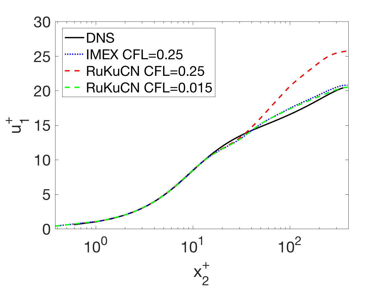
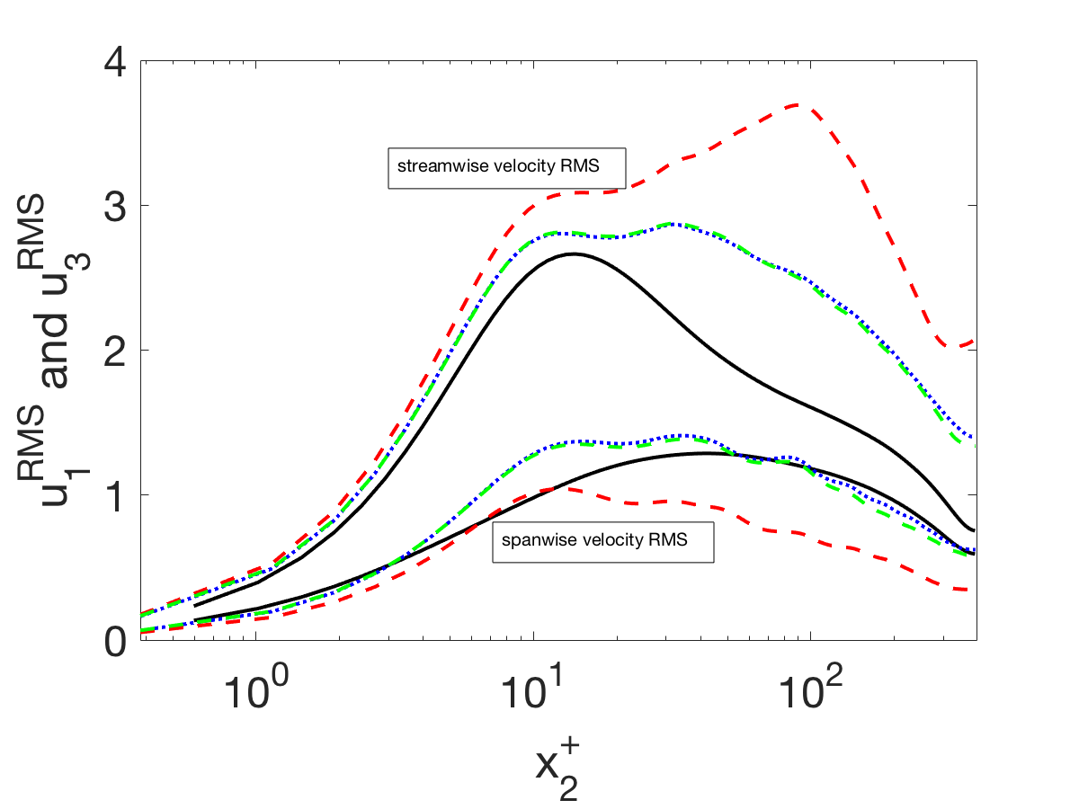
Figure 5: Mean velocity profile (left), as well as streamwise ($u_{2,1}^{\rm RMS}$) and spanwise ($u_{2,3}^{\rm RMS}$) RMS velocity profiles (right).

     

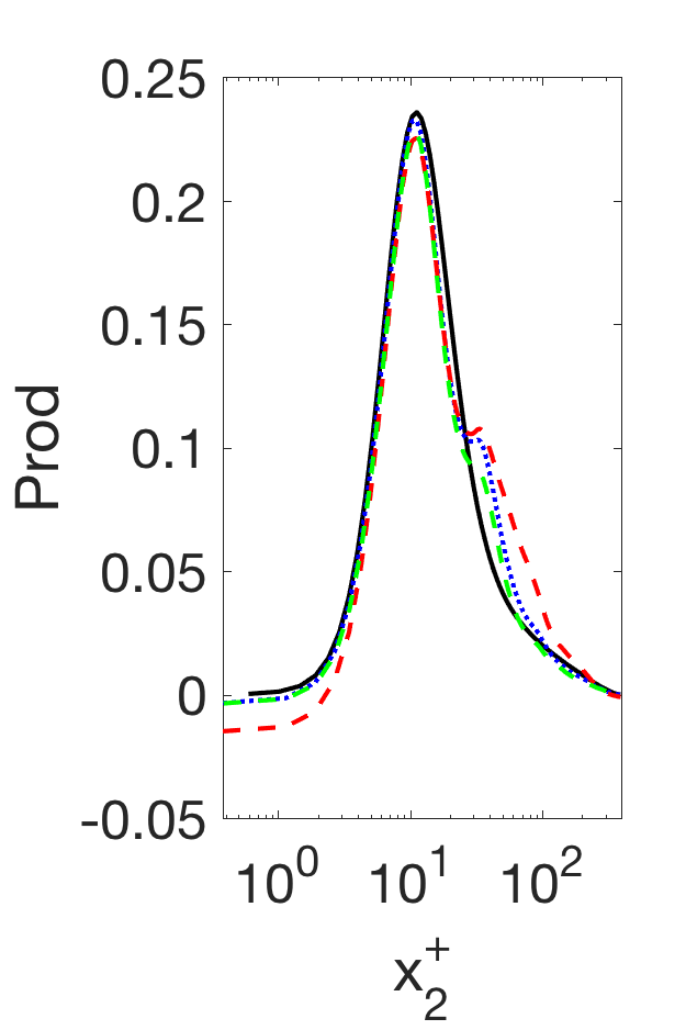
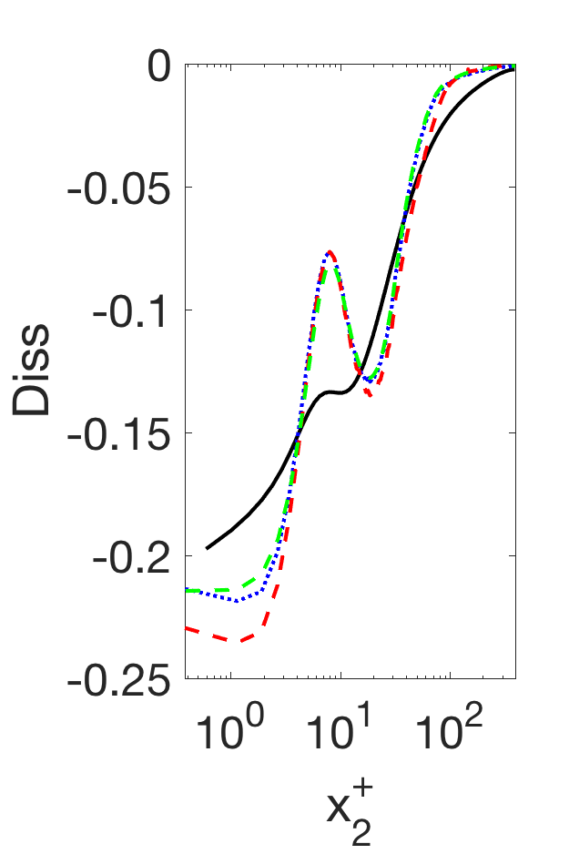
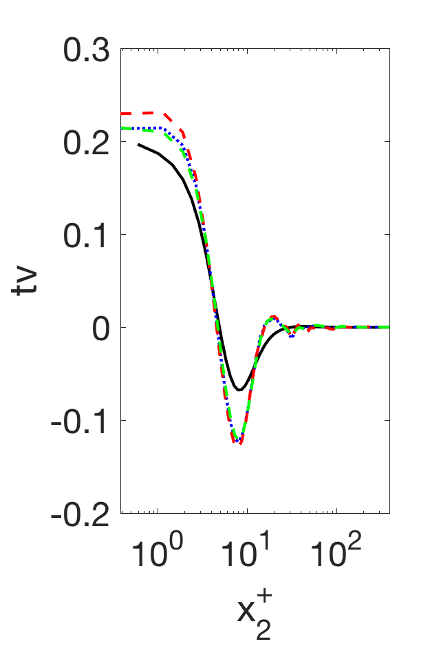
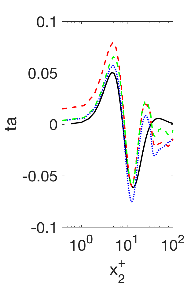
Figure 6: Production ($Prod$), Dissipation ($Diss$), viscous transport ($tv$) and advective transport ($ta$) budgets of the Turbulent Kinetic Energy.

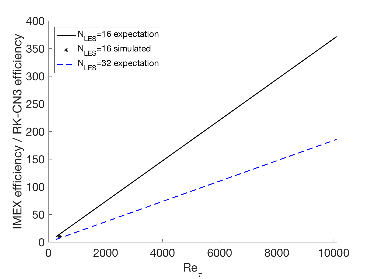
Figure 7: The CN-RK3 CFL number is based on the fine resolution. Thus, the CFL numbers for the IMEX and CN-RK3 schemes increasingly differ for larger Reynolds numbers. As a sidenote, we stress again that in ODTLES the coarse grained grid is kept constant, while the high resolution (with $x_{2}^{+}\leq 1$) is the only one depending on the Reynolds number.

Figure 7 shows a simplified expectation of the increased efficiency of the IMEX scheme in comparison to the CN-RK3 scheme. Here we assume that a sufficient resolution for the wall-normal direction is achieved by satisfying a first cell size $\Delta x_{2}^{+}\leq 1$. This allows highly efficient ODTLES-IMEX computations with moderate and large Reynolds numbers, as it will be shown in the next section.

5.2 Highly Turbulent Channel Flow: IMEX-ODTLES

In a previous work by the author [GlaweThesis2015], ODTLES-CN-RK3 results are presented with $N_{LES}=32$ and $Re_{\tau}=10000$ . Following figure 7, the IMEX scheme should be capable of reaching large Reynolds numbers, even with the performance limitation of a single board computer.

Figure 8 shows results obtained with the IMEX scheme for $Re_{\tau}\leq 2040$. These are in good agreement with the corresponding DNS results from Lee and Moser [Moser:2014, Moser:2015].

The transition of the ODT highly resolved near-wall flow to the 3D LES resolved bulk flow takes place at the coarse grained resolution . The effect can be reduced if some model parameters are adjusted, e.g. the maximum eddy size $l_{max}/\Delta X=1$. $l_{max}$ is the upper threshold for the possible sizes that can be sampled for eddy events during the standalone ODT advancement [WT-Ashurst2005].

 

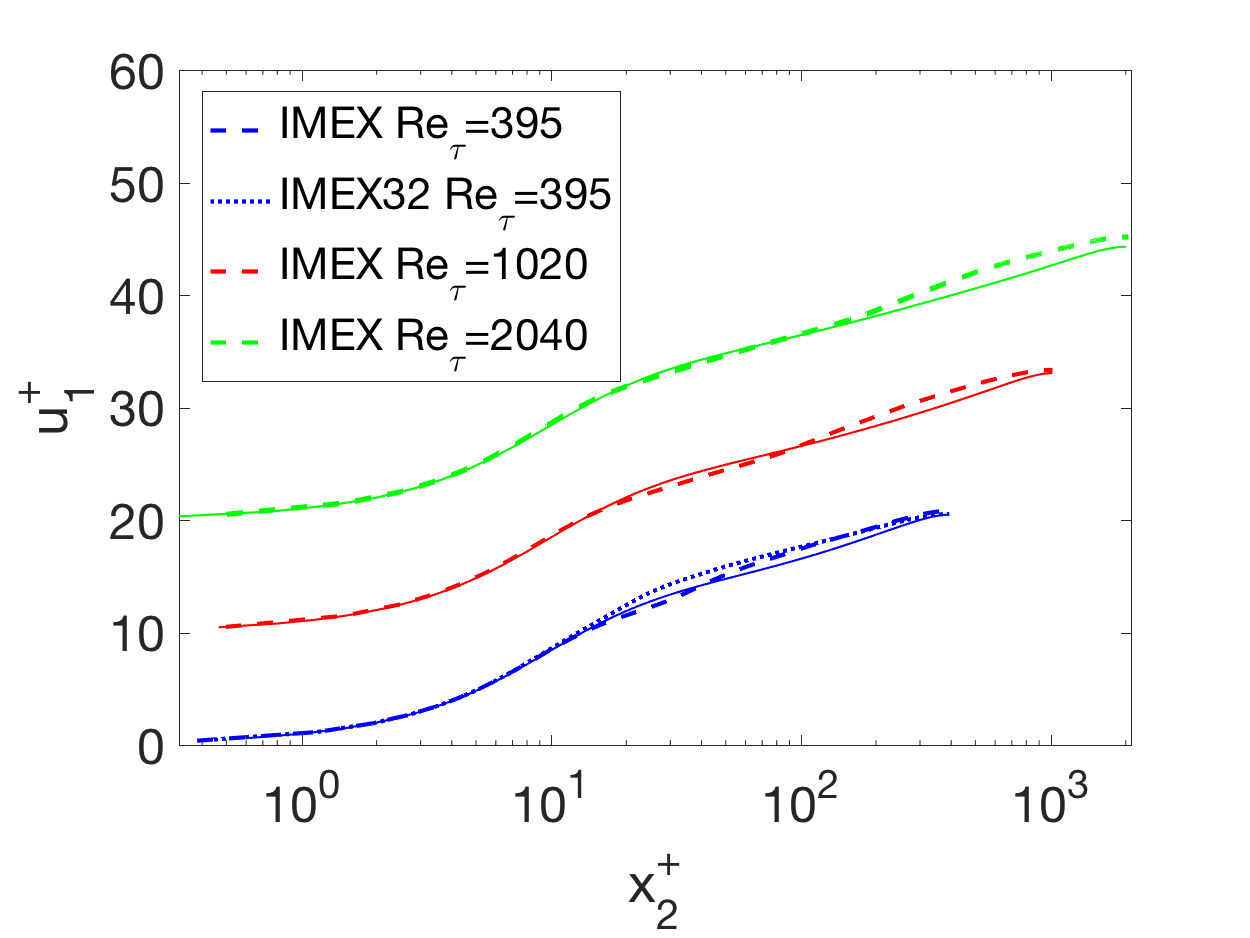
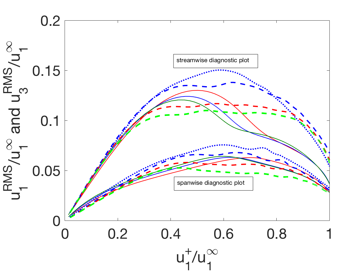
Figure 8: Mean velocity profile showing the logarithmic layer (left). Streamwise ($u_{2,1}^{\rm RMS}$) and spanwise ($u_{2,3}^{\rm RMS}$) RMS velocity profiles are also shown (right) in a diagnostic plot.

6 Summary and Conclusions

In this paper introduce ODTLES, a recent turbulence model applying the One-Dimensional Turbulence (ODT) model as closure within a Large Eddy like model approach. We apply a novel time discretization based on a recent IMEX scheme to the ODTLES model. The IMEX-ODTLES model utilizes the temporal scale separation between the Kolmogorov scale related turbulent ODT advection and the LES based large scale advancement. The resulting scaling properties should hold for other multi-scale problems including atmospheric flows and combustion, where crucial small scale effects in domains of moderate complexity occur.

Turbulent channel flow results show computed with the novel IMEX-ODTLES approach are similar to results based on the previous CN-RK3 implementation, but with significant performance advantage due to increased time-step sizes. This advantage allows to compute an increased turbulent intensity without requiring highly performing hardware.

Appendix A Discretization for ODTLES Spatial Derivative Operators

We dedicate some lines in this Appendix to detail the spatial discretization of the ODTLES derivative operators. Due to the mixing of 1-D and 3-D derivative operators, as well as the existence of three different ODTLES grids as shown in Figure 3, the non-specialized reader may have some difficulties interpreting some of these operators.

We refer now to all of the possible spatial derivative operator cases in the already standard indexing notation $i,j,k$ followed throughout this paper ($i,j,k\in\{1,2,3\}$ with $i\neq j\neq k$; no summation or permutation is implied, unless specified). First, we consider the standard 1-D derivative operators which act exclusively on the ODT line (aligned in direction $k$, or w.l.o.g. in the direction of grid $k$). The 1-D discretization in the line is that of a standard Finite Difference Method for the velocities $u_{k,i}$ ($i,k\in\{1,2,3\}$ with $i\neq k$) stored at the 1-D cell centers. The velocity $u_{k,k}$, nonetheless, is defined at the cell faces. The corresponding derivative operators in this case are the diffusion terms ${\partial^{2}u_{k,i}/\partial x_{k}^{2}}$ ($i,k\in\{1,2,3\}$ with $i\neq k$), which are discretized with a second order Central Difference Method (CDM). For the standard 3-D derivative operators acting on the LES grid, the discretization corresponds to that of a standard staggered grid distribution, with the LES velocities stored at the LES 3-D cell faces and the pressure stored at the cell centers (see Section 3). The corresponding derivative operators in this case are the pressure gradient term $\delta P/\delta X_{l}$ for $l\in\{1,2,3\}$, the LES velocity gradient term (for the pressure correction) $\delta U_{l}/\delta X_{l}$ for $l\in\{1,2,3\}$ and the LES advection terms ${\delta(U_{m}U_{l})/\delta X_{m}}$ for $m\in\{1,2,3\}$ and $l\in\{1,2,3\}\setminus k$ (6 advection derivatives in total, used to calculate the coupling terms, Eq. (18)). Each one of these terms is also discretized with a second order CDM, which, in the case of the advection terms, requires the mutual interpolation of the advecting velocity $U_{m}$ to the interface where $U_{l}$ resides, as well as the interpolation of $U_{l}$ to the cell interfaces that allow the definition of the CDM in $X_{m}$ direction.

An additional category for mixed scale operators arises in ODTLES. These correspond to the advection terms ${\delta(u_{k,i}u_{k,i})/\delta X_{i}}$, ${\delta(u_{k,j}u_{k,i})/\delta X_{j}}$, and ${\partial(u_{k,k}u_{k,i})/\partial x_{k}}$, the velocity gradient terms ${\delta u_{k,i}/\delta X_{i}}$, ${\delta u_{k,j}/\delta X_{j}}$ (for mass conservation, as explained in Section 3.1) and the diffusion term ${\delta^{2}u_{k,i}/\delta X_{i}^{2}}$. In comparison to the standard 1-D or 3-D operators already detailed, confusion may arise in the discretization of these operators.

We begin with the discussion of the velocity gradient terms ${\delta u_{k,i}/\delta X_{i}}$, ${\delta u_{k,j}/\delta X_{j}}$ to illustrate the distribution of fields within ODTLES. These terms are used to enforce mass conservation and determining the velocity field $u_{k,k}$, located at the cell interfaces in the ODT line. In practice it is convenient to define a set of 3 additional indexes $m,n,o$ to refer to the position of a quantity. Therefore, in this section we refer to the quantity $u_{k,i}^{m,n,o}$ as the velocity component $i$ defined in grid $k$, at a discrete position $m,n,o$ in the grid, being $m,n,o$ the discrete counters for the directions $i,j,k$ respectively. A visualization of the values involved in the calculation of $u_{k,k}^{m,n,o}$ can be seen in Figure 9. Table 5 details the discretization of these terms. The velocity $u_{k,k}^{m,n,o}$ is then given by

$$u_{k,k}^{m,n,o}=u_{k,k}^{m,n,o-1}-\left(\frac{u_{k,i}^{m,n,o}-u_{k,i}^{m-1,n,o}}{\Delta X_{i}}+\frac{u_{k,j}^{m,n,o}-u_{k,j}^{m,n-1,o}}{\Delta X_{j}}\right)\Delta x_{k}^{o},$$ (26)

where the $-1$ indexing refers to the elements in the previous line in a certain direction or previous cell within the line.

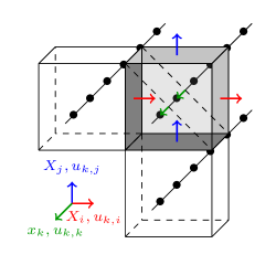
Figure 9: Velocity values required to enforce mass conservation and calculate the value of $u_{k,k}^{m,n,o}$. In general, the quantities $u_{k,i}$ and $u_{k,j}$ defined at the previous lines ($m-1,n-1$) are required, in addition to a previous value $u_{k,k}^{m,n,o-1}$ or a line boundary value. The discretization formula for ${\delta u_{k,i}/\delta X_{i}}$ (or ${\delta u_{k,j}/\delta X_{j}}$) is given in Table 5

Next we discuss the discretization of the diffusion term ${\delta^{2}u_{k,i}/\delta X_{i}^{2}}$. This operator is a direct expansion of the standard CDM involving the quantities in 3 cells along the $X_{i}$ direction. In this case, the cells correspond to those of the neighbour lines directly above and below the cell where $u_{k,i}^{m,n,o}$ is located. A visualization of the values involved in the calculation is shown in Figure 10, while the discretization formula is again given in Table 5.

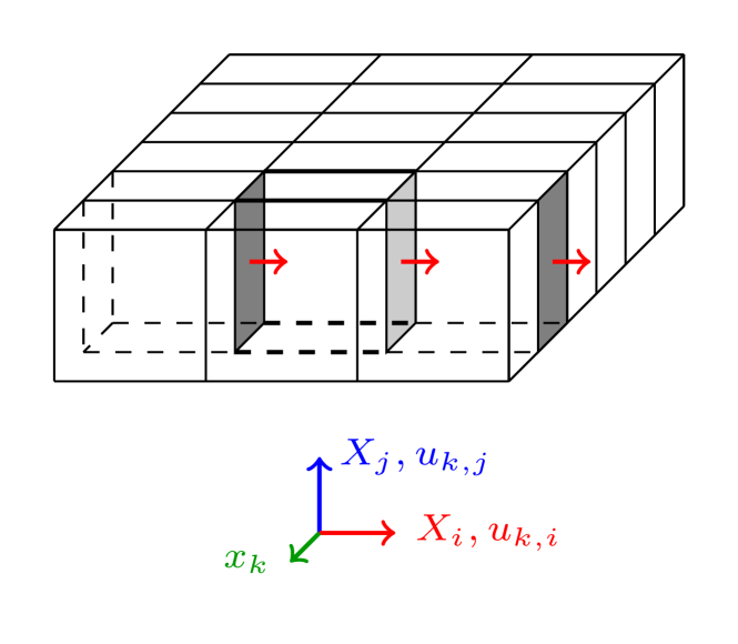
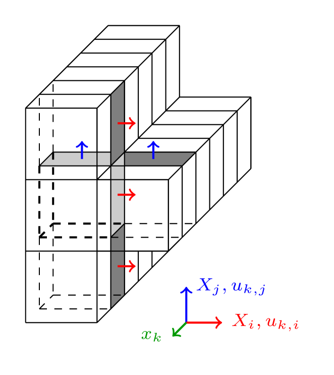
(a)	(b)

Figure 10: (a) Illustration of the velocity values involved in the discretization of the diffusion term ${\delta^{2}u_{k,i}/\delta X_{i}^{2}}$ (neighbour lines $m-1$ and $m+1$ required). (b) Illustration of the velocity values involved in the discretization of the advection term ${\delta(u_{k,j}u_{k,i})/\delta X_{j}}$ (neighbour lines $n-1$ and $n+1$, as well as $m+1$ are required).

The advection terms are discretized analogous to their 3-D LES counterpart. For the advection term ${\delta(u_{k,i}u_{k,i})/\delta X_{i}}$, we construct the CDM for the derivative with the interpolation of the $u_{k,i}$ values to the corresponding LES cell centers in the $X_{i}$ direction. The discretization formula is given in Table 5. This case involves exactly the same values as those required for the diffusion operator described before. In the case of ${\delta(u_{k,j}u_{k,i})/\delta X_{j}}$, $u_{k,j}$ is first interpolated to the interface where $u_{k,i}$ resides, while $u_{k,i}$ is interpolated to the LES cell centers in $X_{j}$ direction in order to construct the CDM (see Figure 10 and Table 5). Finally, the advection term ${\partial(u_{k,k}u_{k,i})/\partial x_{k}}$ is discretized following the same philosophy, where $u_{k,k}$ is first interpolated to the interface where $u_{k,i}$ resides, while $u_{k,i}$ is interpolated to the cell faces in the $x_{k}$ line direction in order to construct the CDM (see Table 5).

Table 5: Discretization formula for special ODTLES derivative operators. In general, the notation $u_{k,i}^{m,n,o}$ refers to the velocity component $i$ defined in grid $k$, at a discrete position $m,n,o$ (or at a cell $o$ in the line located at the 2D position $m,n$ within grid $k$). As usual, $i,j,k\in\{1,2,3\}$ with $i\neq j\neq k$. The terms enclosed in brackets in the derivative term column in the table refer to other terms in the formulation that have an equivalent discretization formula.

Derivative term	Method	Position where	Discretization Formula
		derivative resides
$\frac{\delta u_{k,i}}{\delta X_{i}}$ $\Big{(}$ or $\frac{\delta u_{k,j}}{\delta X_{j}}$ $\Big{)}$	CDM	Cell center $o$	$\frac{u_{k,i}^{m,n,o}-u_{k,i}^{m-1,n,o}}{\Delta X_{i}}$
$\frac{\delta^{2}u_{k,i}}{\delta X_{i}^{2}}$	CDM	Center of cell face $m$	$\frac{u_{k,i}^{m-1,n,o}-2u_{k,i}^{m,n,o}+u_{k,i}^{m+1,n,o}}{\Delta X_{i}^{2}}$
$\frac{\delta u_{k,i}u_{k,i}}{\delta X_{i}}$ $\Big{(}\frac{\delta u_{k,j}u_{k,j}}{\delta X_{j}}\Big{)}$	CDM	Center of cell face $m$	$\frac{1}{\Delta X_{i}}\left[\left(\frac{u_{k,i}^{m+1,n,o}+u_{k,i}^{m,n,o}}{2}\right)^{2}-\left(\frac{u_{k,i}^{m,n,o}+u_{k,i}^{m-1,n,o}}{2}\right)^{2}\right]$
$\frac{\delta u_{k,j}u_{k,i}}{\delta X_{j}}$ $\Big{(}\frac{\delta u_{k,i}u_{k,j}}{\delta X_{i}}\Big{)}$	CDM	Center of cell face $m$	$\frac{1}{\Delta X_{j}}\Bigg{[}\left(\frac{u_{k,j}^{m+1,n,o}+u_{k,j}^{m,n,o}}{2}\right)\left(\frac{u_{k,i}^{m,n+1,o}+u_{k,i}^{m,n,o}}{2}\right)$
			$-\left(\frac{u_{k,j}^{m+1,n,o}+u_{k,j}^{m,n,o}}{2}\right)\left(\frac{u_{k,i}^{m,n,o}+u_{k,i}^{m,n-1,o}}{2}\right)\Bigg{]}$
$\frac{\partial u_{k,k}u_{k,i}}{\partial x_{k}}$ $\Big{(}\frac{\partial u_{k,k}u_{k,j}}{\partial x_{k}}\Big{)}$	CDM	Center of cell face $m$	$\frac{1}{\Delta x_{k}}\Bigg{[}\left(\frac{u_{k,k}^{m+1,n,o}+u_{k,k}^{m,n,o}}{2}\right)\left(\frac{u_{k,i}^{m,n,o+1}+u_{k,i}^{m,n,o}}{2}\right)$
			$-\left(\frac{u_{k,k}^{m+1,n,o}+u_{k,k}^{m,n,o}}{2}\right)\left(\frac{u_{k,i}^{m,n,o}+u_{k,i}^{m,n,o-1}}{2}\right)\Bigg{]}$

Appendix B Implementation details for IMEX-ODTLES Time Advancement

In this Appendix we give further details regarding the implementation of the IMEX-ODTLES time scheme introduced in Table 3 for the channel flow simulations. As in any time-advancement scheme, the algorithm begins with the input of suitable initial conditions and the calculation of the time-step. For the ODTLES IMEX scheme, the magnitude of the time-step is calculated by means of Eq. (25), i.e. the LES time-step $\Delta T$.

We now revise each substep in Table 3 and annotate relevant comments, if necessary. We use the index $n$ in this section, just as in Table 3, to refer to the discrete time-levels during the advancement.

• Substep p $1.1$: The explicit RHS $R_{EX}(u_{k,i})$ calculates all the explicit terms in the function $g(u_{k,i},t)$ in Eq. (24). The eddy transformation function $\mathit{eddy}_{k,i}$ and the terms within brackets in Eq. (24) are first neglected. The pre-emptive RHS is stored and input as a constant term in the first standalone ODT advancement in the scheme (the original channel flow forcing term in streamwise direction is also given as a constant input). As detailed in [WT-Ashurst2005], an eddy sampling from $t=t_{start}$ to $t=t_{end}=\Delta T$ takes place by evaluating eddies with sampled size $l$ (from an assumed eddy-size PDF) and position $x_{0}$ (from a uniform distribution) at eddy occurrence times following a Poisson process with a pre-specified mean rate. Eddies can be accepted or rejected in a Bernoulli trial based on the calculation of the ODT eddy turnover time $\tau_{e}$ [WT-Ashurst2005]. If an eddy is deemed to be accepted and implemented, a catchup diffusion event takes place. This catchup diffusion event is nothing more than the time-advancement in the line (according to the fine-scale CFL condition) of Eq. (3), thus incorporates the missing bracket terms in Eq. (24) neglected so far. Once the ODT advancement is finalized, the explicit RHS $R_{EX}(u_{k,i})$ is calculated (and stored) using the resultant velocity field at time level $n_{end}$ and the starting velocity field at time level $n_{start}$,

  $$R=\frac{u_{k,i}^{n_{end}}-u_{k,i}^{n_{start}}}{\Delta t_{n_{start},n_{end}}}.$$ (27)

• Substep p $\mathbf{1.2}$: The equation $\partial u_{k,i}/\partial t=f(u_{k,i},t)$ is solved in this step, for the implicit RHS $f(u_{k,i},t)$ given by Eq. (23). The discretization for the $\frac{\partial u_{k,k}u_{k,i}}{\partial x_{k}}$ term was given in A. It is important to note that, since the interpolation of $u_{k,k}$ values to cell interfaces requires information residing outside the ODT line, the interpolated $u_{k,k}$ is computed by means of mass conservation, Eq. (26), prior to the advancement, and considered constant during the implicit solution procedure. In this work, the implicit solution (based entirely on information residing in one ODT line) is calculated by means of a Tri-Diagonal Matrix Algorithm (TDMA). After the calculation of the resultant velocity field, the implicit RHS is calculated by means of Eq. (27) and subsequently stored.

• Substep p $\mathbf{1.3}$: The explicit RHS computed and stored in p $1.1$ and the implicit RHS computed and stored in p $1.2$ are synchronously advanced in an explicit Euler step. After this step the explicit and implicit treated terms have the same time level.

• Substep p $\mathbf{1.4}$: The coupling terms are calculated and advanced with an explicit Euler scheme along with the forcing and large scale diffusion terms. Note that the ODT coupling term given by Eq. (17) does not consider neither the forcing nor the large scale diffusion in order to avoid double counting of these terms. Therefore, the explicit RHS calculated in substep p $1.3$ must be modified accordingly, prior to the transmission from grid $j$ to grid $k$.

• Substep c $\mathbf{1.1}$: LES cell-size averages are calculated in all ODT lines and used to construct the LES velocity field. At this point, the consistency condition given by Eq. (11) is observed. It is not important to give priority to the average of one velocity component in one grid over another (it is also not necessary to do an average of the filtered velocity fields in both grids where they are available, as it was done in previous works [ED-Gonzalez-Juez2011]).

• Substep c $\mathbf{1.2}$: The hydrodynamic pressure is determined in each cell in order to enforce divergence-free LES velocity fields, Eq. (15). The pressure Poisson equation is solved in this work using the Algebraic Multi-Grid (AMG) solver of the hypre distribution package [Falgout02hypre:a].

• Substep c $\mathbf{1.3}$: The LES velocity field is corrected with the calculated values of the hydrodynamic pressure.

• Substep c $\mathbf{1.4}$: The downscaling operation [GlaweThesis2015] is applied to reconstruct the highly-resolved fields $u_{k,i}$ and $u_{k,j}$ residing in each grid $k$ (this gives a total of 6 downscaling operations). There is a duplicity of each large scale velocity component, since one velocity component resides in two different ODTLES grids.

• Substep c $\mathbf{1.5}$: The advancing velocity components required for the next IMEX subcycle are computed. In each grid the available two velocities are used. The third velocity component follows from the incompressibility constrain.

• Substep p $\mathbf{2.1}$: Explicit Euler advancement using the last stored values for the explicit and implicit RHS. The implicit RHS is not advanced due to the cancellation of time-advancement coefficients.

• Substep p $\mathbf{2.2}$: Substep p $1.2$ is repeated with the currently available velocity field.

• From Substep p $\mathbf{2.3}$ to substep c $\mathbf{2.5}$: Substeps p $1.3$ to c $1.5$ are repeated considering the different RHS terms and time advancement coefficients following Table 2. The velocity field obtained at the end of substep c $2.4$ is the velocity field at the new time-step $t+\Delta T$.