Sequential Attend, Infer, Repeat: Generative Modelling of Moving Objects

Abstract

We present Sequential Attend, Infer, Repeat (sqair), an interpretable deep generative model for videos of moving objects. It can reliably discover and track objects throughout the sequence of frames, and can also generate future frames conditioning on the current frame, thereby simulating expected motion of objects. This is achieved by explicitly encoding object presence, locations and appearances in the latent variables of the model. Sqair retains all strengths of its predecessor, Attend, Infer, Repeat (air, [9]), including learning in an unsupervised manner, and addresses its shortcomings. We use a moving multi-mnist dataset to show limitations of AIR in detecting overlapping or partially occluded objects, and show how sqair overcomes them by leveraging temporal consistency of objects. Finally, we also apply sqair to real-world pedestrian CCTV data, where it learns to reliably detect, track and generate walking pedestrians with no supervision.

1 Introduction

The ability to identify objects in their environments and to understand relations between them is a cornerstone of human intelligence [21]. Arguably, in doing so we rely on a notion of spatial and temporal consistency which gives rise to an expectation that objects do not appear out of thin air, nor do they spontaneously vanish, and that they can be described by properties such as location, appearance and some dynamic behaviour that explains their evolution over time. We argue that this notion of consistency can be seen as an inductive bias that improves the efficiency of our learning. Equally, we posit that introducing such a bias towards spatio-temporal consistency into our models should greatly reduce the amount of supervision required for learning.

One way of achieving such inductive biases is through model structure. While recent successes in deep learning demonstrate that progress is possible without explicitly imbuing models with interpretable structure [27], recent works show that introducing such structure into deep models can indeed lead to favourable inductive biases improving performance e.g. in convolutional networks [28] or in tasks requiring relational reasoning [36]. Structure can also make neural networks useful in new contexts by significantly improving generalization, data efficiency [19] or extending their capabilities to unstructured inputs [11].

Attend, Infer, Repeat (air), introduced by [9], is a notable example of such a structured probabilistic model that relies on deep learning and admits efficient amortized inference. Trained without any supervision, air is able to decompose a visual scene into its constituent components and to generate a (learned) number of latent variables that explicitly encode the location and appearance of each object. While this approach is inspiring, its focus on modelling individual (and thereby inherently static) scenes leads to a number of limitations. For example, it often merges two objects that are close together into one since no temporal context is available to distinguish between them. Similarly, we demonstrate that air struggles to identify partially occluded objects, e.g. when they extend beyond the boundaries of the scene frame (see Figure 7 in Section 4.1).

Our contribution is to mitigate the shortcomings of air by introducing a sequential version that models sequences of frames, enabling it to discover and track objects over time as well as to generate convincing extrapolations of frames into the future. We achieve this by leveraging temporal information to learn a richer, more capable generative model. Specifically, we extend air into a spatio-temporal state-space model and train it on unlabelled image sequences of dynamic objects. We show that the resulting model, which we name Sequential air (sqair), retains the strengths of the original AIR formulation while outperforming it on moving mnist digits.

The rest of this work is organised as follows. In Section 2, we describe the generative model and inference of air. In Section 3, we discuss its limitations and how it can be improved, thereby introducing Sequential Attend, Infer, Repeat (sqair), our extension of air to image sequences. In Section 4, we demonstrate the model on a dataset of multiple moving MNIST digits (Section 4.1) and compare it against air trained on each frame and Variational Recurrent Neural Network (vrnn) of [5] with convolutional architectures, and show the superior performance of sqair in terms of log marginal likelihood and interpretability of latent variables. We also investigate the utility of inferred latent variables of sqair in downstream tasks. In Section 4.2 we apply sqair on real-world pedestrian CCTV data, where sqair learns to reliably detect, track and generate walking pedestrians without any supervision. Code for the implementation on the mnist dataset and the results video are available online.

2 Attend, Infer, Repeat (AIR)

air, introduced by [9], is a structured variational auto-encoder (vae) capable of decomposing a static scene $\mathbf{x}$ into its constituent objects, where each object is represented as a separate triplet of continuous latent variables $\mathbf{z}=\{\mathbf{z}^{\mathrm{what},i},\mathbf{z}^{\mathrm{where},i},z^{\mathrm{pres},i}\}_{i=1}^{n}$, $n\in\mathbb{N}$ being the (random) number of objects in the scene. Each triplet of latent variables explicitly encodes position, appearance and presence of the respective object, and the model is able to infer the number of objects present in the scene. Hence it is able to count, locate and describe objects in the scene, all learnt in an unsupervised manner, made possible by the inductive bias introduced by the model structure.

Generative Model The generative model of air is defined as follows

$$p_{\theta}\left(n\right) =\mathrm{Geom}(n\mid\theta), p_{\theta}\left(\mathbf{z}^{\mathrm{w}}\mid n\right) =\prod_{i=1}^{n}p_{\theta}\left(\mathbf{z}^{w,i}\right)=\prod_{i=1}^{n}{\mathcal{N}\left(\mathbf{z}^{w,i}|\bf{0},\bf{I}\right)},$$

$$p_{\theta}\left(\mathbf{x}\mid\mathbf{z}\right) ={\mathcal{N}\left(\mathbf{x}\mid\mathbf{y}_{t},\sigma^{2}_{x}\bm{I}\right)}, \text{with}~{}~{}\mathbf{y}_{t} =\sum_{i=1}^{n}\operatorname{h}^{\mathrm{dec}}_{\theta}(\mathbf{z}^{\mathrm{what},i},\mathbf{z}^{\mathrm{where},i}),$$ (1)

where $\mathbf{z}^{\mathrm{w},i}\mathrel{\vbox{\hbox{.}\hbox{.}}}=(\mathbf{z}^{\mathrm{what},i},\mathbf{z}^{\mathrm{where},i})$, $z^{\mathrm{pres},i}=1$ for $i=1\ldots n$ and $h^{\mathrm{dec}}_{\theta}$ is the object decoder with parameters $\theta$. It is composed of a glimpse decoder $f_{\theta}^{\mathrm{dec}}:\mathbf{g}_{t}^{i}\mapsto\mathbf{y}_{t}^{i}$, which constructs an image patch and a spatial transformer ($\operatorname{ST}$, [20]), which scales and shifts it according to $\mathbf{z}^{\mathrm{where}}$; see Figure 1 for details.

Inference [9] use a sequential inference algorithm, where latent variables are inferred one at a time; see Figure 2. The number of inference steps $n$ is given by $z^{\mathrm{pres},1:n+1}$, a random vector of $n$ ones followed by a zero. The $\mathbf{z}^{i}$ are sampled sequentially from

$$q_{\phi}\left(\mathbf{z}\mid\mathbf{x}\right)=q_{\phi}\left(z^{\mathrm{pres},n+1}=0\mid\mathbf{z}^{\mathrm{w},1:n},\mathbf{x}\right)\prod_{i=1}^{n}q_{\phi}\left(\mathbf{z}^{\mathrm{w},i},z^{\mathrm{pres},i}=1\mid\mathbf{z}^{1:i-1},\mathbf{x}\right),$$ (2)

where $q_{\phi}$ is implemented as a neural network with parameters $\phi$. To implement explaining away, e.g. to avoid encoding the same object twice, it is vital to capture the dependency of $\mathbf{z}^{\mathrm{w},i}$ and $z^{\mathrm{pres},i}$ on $\mathbf{z}^{1:i-1}$ and $\mathbf{x}$. This is done using a recurrent neural network (rnn) $R_{\phi}$ with hidden state $\bm{h}^{i}$, namely: $\bm{\omega}^{i},\bm{h}^{i}=R_{\phi}(\mathbf{x},\mathbf{z}^{i-1},\bm{h}^{i-1}).$ The outputs $\bm{\omega}^{i}$, which are computed iteratively and depend on the previous latent variables (cf. Algorithm 3), parametrise $q_{\phi}\left(\mathbf{z}^{\mathrm{w},i},\mathbf{z}^{\mathrm{pres},i}\mid\mathbf{z}^{1:i-1},\mathbf{x}\right)$. For simplicity the latter is assumed to factorise such that $q_{\phi}\left(\mathbf{z}^{\mathrm{w}},\mathbf{z}^{\mathrm{pres}}\mid\mathbf{z}^{1:i-1},\mathbf{x}\right)=q_{\phi}\left(z^{\mathrm{pres},n+1}=0\mid\bm{\omega}^{n+1}\right)\prod_{i=1}^{n}q_{\phi}\left(\mathbf{z}^{\mathrm{w},i}\mid\bm{\omega}^{i}\right)q_{\phi}\left(z^{\mathrm{pres},i}=1\mid\bm{\omega}^{i}\right).$

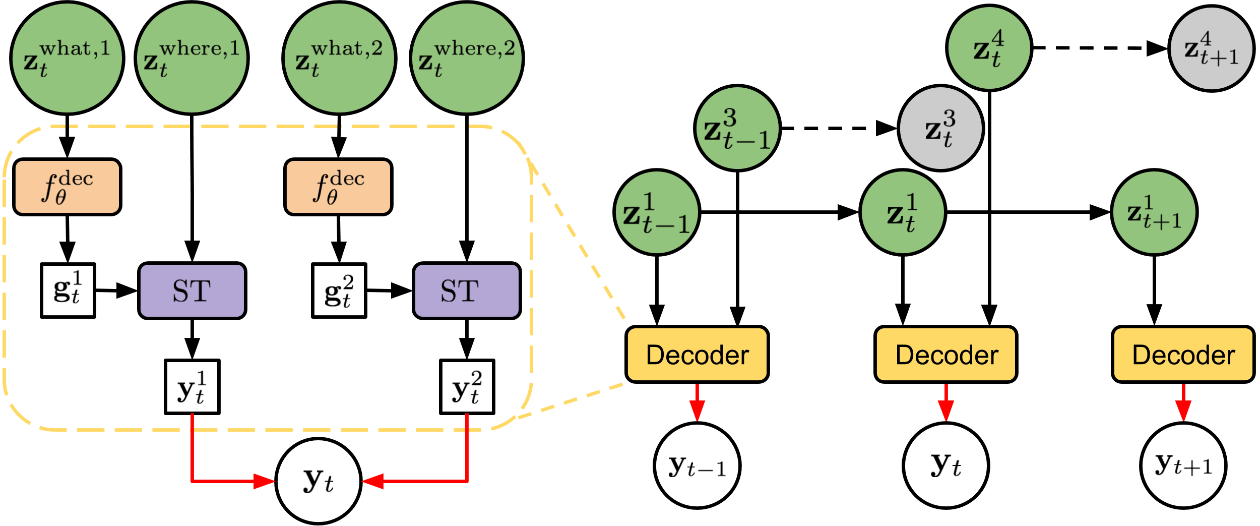
Figure 1: Left: Generation in air. The image mean $\mathbf{y}_{t}$ is generated by first using the glimpse decoder $f_{\theta}^{\mathrm{dec}}$ to map the what variables into glimpses $\mathbf{g}_{t}$, transforming them with the spatial transformer $\operatorname{ST}$ according to the where variables and summing up the results. Right: Generation in sqair. When new objects enter the frame, new latent variables (here, $\mathbf{z}_{t}^{4}$) are sampled from the discovery prior. The temporal evolution of already present objects is governed by the propagation prior, which can choose to forget some variables (here, $\mathbf{z}_{t}^{3}$ and $\mathbf{z}_{t+1}^{4}$) when the object moves out of the frame. The image generation process, which mimics the left-hand side of the figure, is abstracted in the decoder block.

3 Sequential Attend-Infer-Repeat

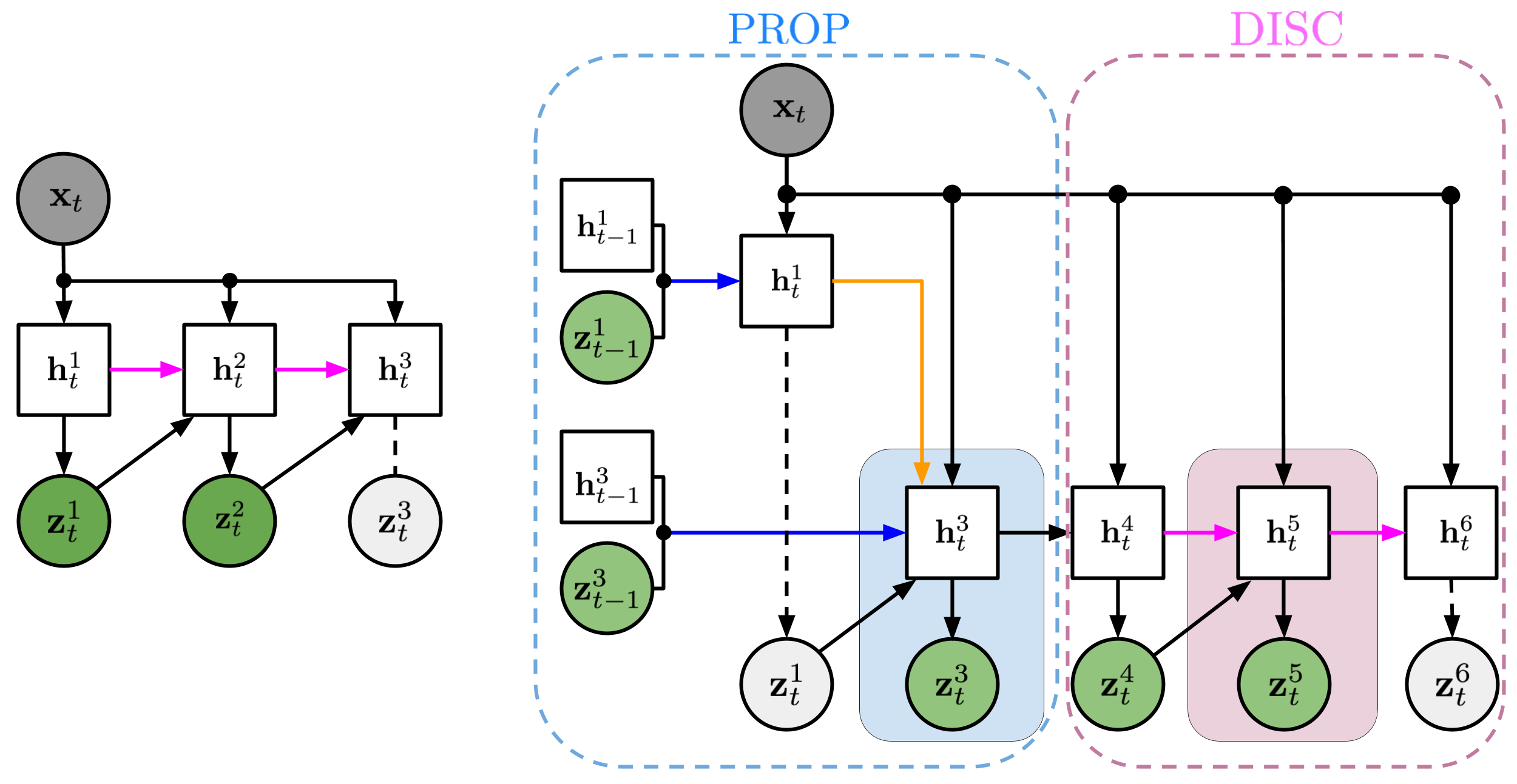
Figure 2: Left: Inference in air. The pink rnn attends to the image sequentially and produces one latent variable $\mathbf{z}_{t}^{i}$ at a time. Here, it decides that two latent variables are enough to explain the image and $\mathbf{z}_{t}^{3}$ is not generated. Right: Inference in sqair starts with the prop phase. prop iterates over latent variables from the previous time-step $t-1$ and updates them based on the new observation $\mathbf{x}_{t}$. The blue rnn runs forward in time to update the hidden state of each object, to model its change in appearance and location throughout time. The orange rnn runs across all current objects and models the relations between different objects. Here, when attending to $\mathbf{z}^{1}_{t-1}$, it decides that the corresponding object has disappeared from the frame and forgets it. Next, the disc phase detects new objects as in air, but in sqair it is also conditioned on the results of prop, to prevent rediscovering objects. See Figure 3 for details of the colored RNNs.

While capable of decomposing a scene into objects, air only describes single images. Should we want a similar decomposition of an image sequence, it would be desirable to do so in a temporally consistent manner. For example, we might want to detect objects of the scene as well as infer dynamics and track identities of any persistent objects. Thus, we introduce Sequential Attend, Infer, Repeat (sqair), whereby air is augmented with a state-space model (ssm) to achieve temporal consistency in the generated images of the sequence. The resulting probabilistic model is composed of two parts: Discovery (disc), which is responsible for detecting (or introducing, in the case of the generation) new objects at every time-step (essentially equivalent to air), and Propagation (prop), responsible for updating (or forgetting) latent variables from the previous time-step given the new observation (image), effectively implementing the temporal ssm. We now formally introduce sqair by first describing its generative model and then the inference network.

Generative Model The model assumes that at every-time step, objects are first propagated from the previous time-step (prop). Then, new objects are introduced (disc). Let $t\in\mathbb{N}$ be the current time-step. Let $\mathcal{P}_{t}$ be the set of objects propagated from the previous time-step and let $\mathcal{D}_{t}$ be the set of objects discovered at the current time-step, and let $\mathcal{O}_{t}=\mathcal{P}_{t}\cup\mathcal{D}_{t}$ be the set of all objects present at time-step $t$. Consequently, at every time step, the model retains a set of latent variables $\mathbf{z}_{t}^{\mathcal{P}_{t}}=\{\mathbf{z}_{t}^{i}\}_{i\in\mathcal{P}_{t}}$, and generates a set of new latent variables $\mathbf{z}_{t}^{\mathcal{D}_{t}}=\{\mathbf{z}_{t}^{i}\}_{i\in\mathcal{D}_{t}}$. Together they form $\mathbf{z}_{t}\mathrel{\vbox{\hbox{.}\hbox{.}}}=[\mathbf{z}_{t}^{\mathcal{P}_{t}},\mathbf{z}_{t}^{\mathcal{D}_{t}}]$, where the representation of the $i^{\mathrm{th}}$ object $\mathbf{z}_{t}^{i}\mathrel{\vbox{\hbox{.}\hbox{.}}}=[\mathbf{z}_{t}^{\mathrm{what},i},\mathbf{z}_{t}^{\mathrm{where},i},z_{t}^{\mathrm{pres},i}]$ is composed of three components (as in air): $\mathbf{z}_{t}^{\mathrm{what},i}$ and $\mathbf{z}_{t}^{\mathrm{where},i}$ are real vector-valued variables representing appearance and location of the object, respectively. $z_{t}^{\mathrm{pres},i}$ is a binary variable representing whether the object is present at the given time-step or not.

At the first time-step ($t=1$) there are no objects to propagate, so we sample $D_{1}$, the number of objects at $t=1$, from the discovery prior $p^{D}\left(D_{1}\right)$. Then for each object $i\in\mathcal{D}_{t}$, we sample latent variables $\mathbf{z}_{t}^{\mathrm{what},i},\mathbf{z}_{t}^{\mathrm{where},i}$ from $p^{D}\left(z_{1}^{i}\mid D_{1}\right)$. At time $t=2$, the propagation step models which objects from $t=1$ are propagated to $t=2$, and which objects disappear from the frame, using the binary random variable $(z_{t}^{\mathrm{pres},i})_{i\in\mathcal{P}_{t}}$. The discovery step at $t=2$ models new objects that enter the frame, with a similar procedure to $t=1$: sample $D_{2}$ (which depends on $\mathbf{z}_{2}^{\mathcal{P}_{2}}$) then sample $(\mathbf{z}_{2}^{\mathrm{what},i},\mathbf{z}_{2}^{\mathrm{where},i})_{i\in\mathcal{D}_{2}}$. This procedure of propagation and discovery recurs for $t=2,\ldots T$. Once the $\mathbf{z}_{t}$ have been formed, we may generate images $\mathbf{x}_{t}$ using the exact same generative distribution $p_{\theta}\left(\mathbf{x}_{t}\mid\mathbf{z}_{t}\right)$ as in air (cf. Sections 2, 1 and 1). In full, the generative model is:

$$p(\mathbf{x}_{1:T},\mathbf{z}_{1:T},D_{1:T})=p^{D}(D_{1},\mathbf{z}_{1}^{\mathcal{D}_{1}})\prod_{t=2}^{T}p^{D}(D_{t},\mathbf{z}_{t}^{\mathcal{D}_{t}}|\mathbf{z}_{t}^{\mathcal{P}_{t}})p^{P}(\mathbf{z}_{t}^{\mathcal{P}_{t}}|\mathbf{z}_{t-1})p_{\theta}(\mathbf{x}_{t}|\mathbf{z}_{t}),$$ (3)

The discovery prior $p^{D}(D_{t},\mathbf{z}_{t}^{\mathcal{D}_{t}}|\mathbf{z}_{t}^{\mathcal{P}_{t}})$ samples latent variables for new objects that enter the frame. The propagation prior $p^{P}(\mathbf{z}_{t}^{\mathcal{P}_{t}}|\mathbf{z}_{t-1})$ samples latent variables for objects that persist in the frame and removes latents of objects that disappear from the frame, thereby modelling dynamics and appearance changes. Both priors are learned during training. The exact forms of the priors are given in Appendix B.

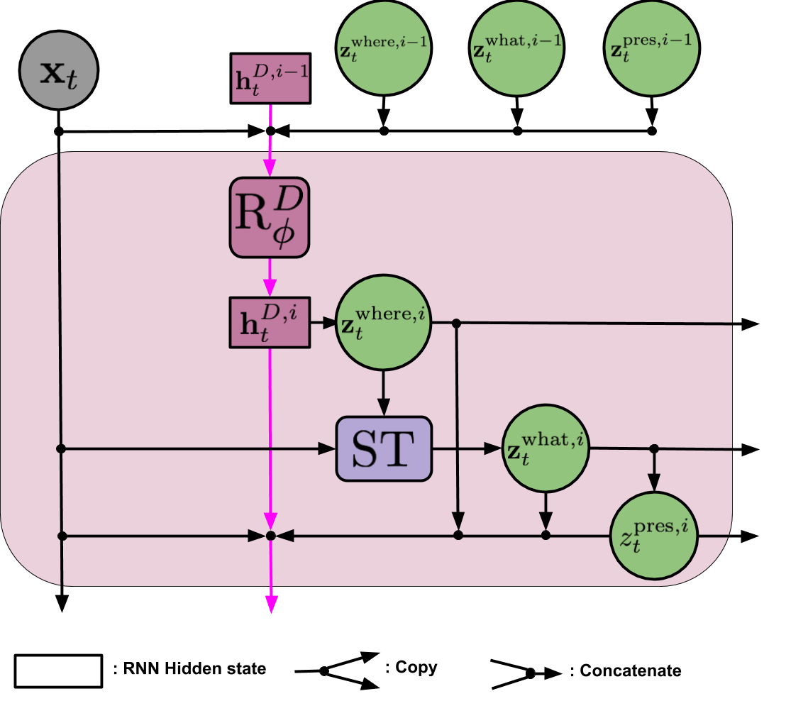
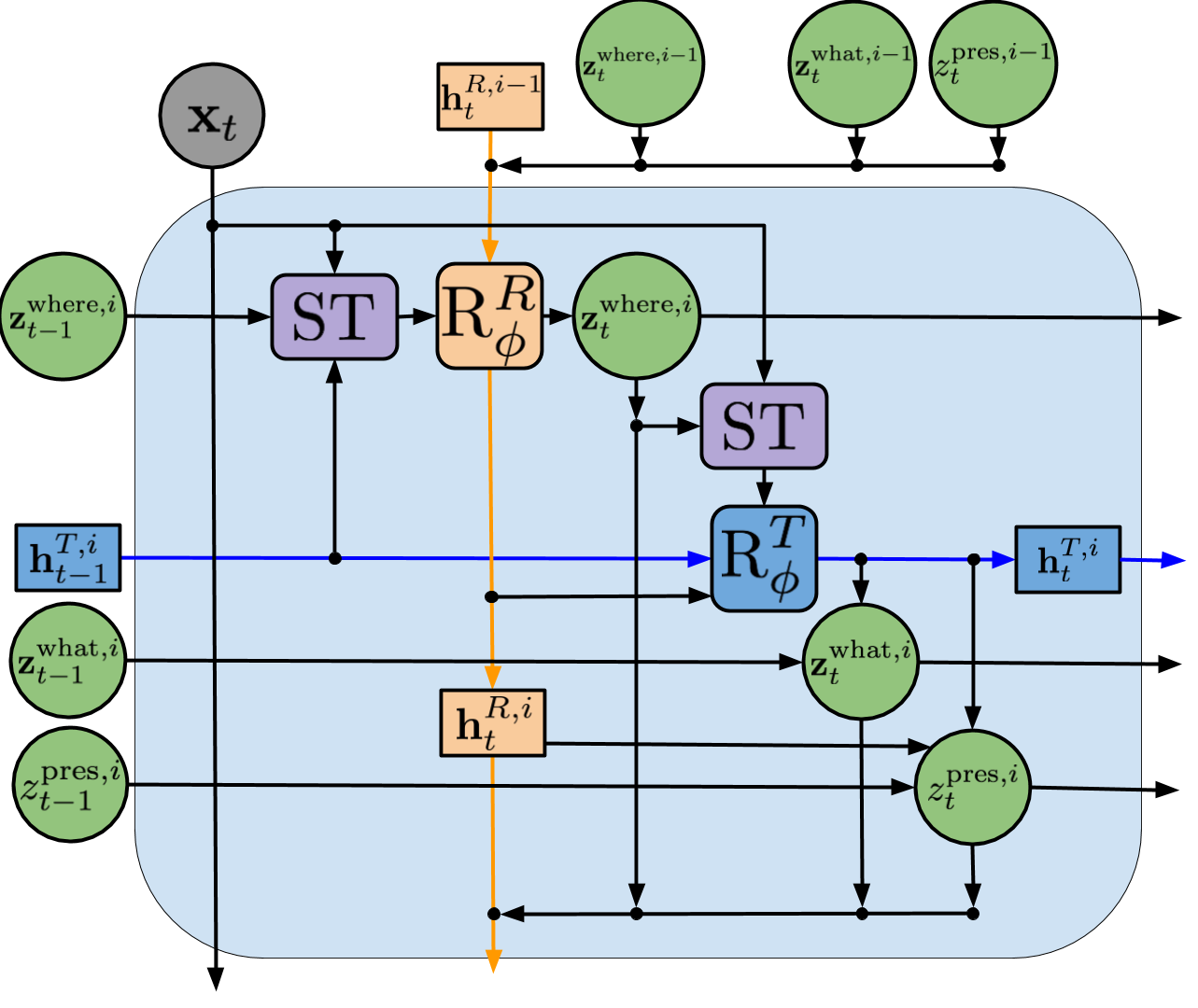
Figure 3: Left: Interaction between prop and disc in sqair. Firstly, objects are propagated to time $t$, and object $i=7$ is dropped. Secondly, disc tries to discover new objects. Here, it manages to find two objects: $i=9$ and $i=10$. The process recurs for all remaining time-steps. Blue arrows update the temporal hidden state, orange ones infer relations between objects, pink ones correspond to discovery. Bottom: Information flow in a single discovery block (left) and propagation block (right). In disc we first predict where and extract a glimpse. We then predict what and presence. Prop starts with extracting a glimpse at a candidate location and updating where. Then it follows a procedure similar to disc, but takes the respective latent variables from the previous time-step into account. It is approximately two times more computationally expensive than disc. For details, see Algorithms 2 and 3 in Appendix A.

Inference Similarly to air, inference in sqair can capture the number of objects and the representation describing the location and appearance of each object that is necessary to explain every image in a sequence. As with generation, inference is divided into prop and disc. During prop, the inference network achieves two tasks. Firstly, the latent variables from the previous time step are used to infer the current ones, modelling the change in location and appearance of the corresponding objects, thereby attaining temporal consistency. This is implemented by the temporal rnn ${\color[rgb]{0,0,1}\operatorname{R}_{\phi}^{T}}$, with hidden states ${\color[rgb]{0,0,1}\bm{h}_{t}^{T}}$ (recurs in $t$). Crucially, it does not access the current image directly, but uses the output of the relation rnn (cf. [36]). The relation rnn takes relations between objects into account, thereby implementing the explaining away phenomenon; it is essential for capturing any interactions between objects as well as occlusion (or overlap, if one object is occluded by another). See Figure 7 for an example. These two rnn s together decide whether to retain or to forget objects that have been propagated from the previous time step. During disc, the network infers further latent variables that are needed to describe any new objects that have entered the frame. All latent variables remaining after prop and disc are passed on to the next time step.

See Figures 2 and 3 for the inference network structure . The full variational posterior is defined as

$$q_{\phi}\left(D_{1:t},\mathbf{z}_{1:T}\mid\mathbf{x}_{1:T}\right)=\prod_{t=1}^{T}q^{D}_{\phi}\left(D_{t},\mathbf{z}_{t}^{\mathcal{D}_{t}}\mid\mathbf{x}_{t},\mathbf{z}_{t}^{\mathcal{P}_{t}}\right)\prod_{i\in\mathcal{O}_{t-1}}q^{P}_{\phi}\left(\mathbf{z}_{t}^{i}\mid\mathbf{z}_{t-1}^{i},{\color[rgb]{0,0,1}\bm{h}_{t}^{T,i}},{\color[rgb]{1,0.6015625,0}\bm{h}_{t}^{R,i}}\right).$$ (4)

Discovery, described by $q^{D}_{\phi}$, is very similar to the full posterior of air, cf. Equation 2. The only difference is the conditioning on $\mathbf{z}_{t}^{\mathcal{P}_{t}}$, which allows for a different number of discovered objects at each time-step and also for objects explained by prop not to be explained again. The second term, or $q^{P}_{\phi}$, describes propagation. The detailed structures of $q^{D}_{\phi}$ and $q^{P}_{\phi}$ are shown in Figure 3, while all the pertinent algorithms and equations can be found in Appendices A and C, respectively.

Learning We train sqair as an importance-weighted auto-encoder (iwae) of [3]. Specifically, we maximise the importance-weighted evidence lower-bound $\mathcal{L}_{\textsc{IWAE}}$, namely

$$\mathcal{L}_{\textsc{IWAE}}=\mathbb{E}_{\mathbf{x}_{1:T}\sim p_{\mathrm{data}}\left(\mathbf{x}_{1:T}\right)}\left[\mathbb{E}_{q}\left[\log\frac{1}{K}\sum_{k=1}^{K}\frac{p_{\theta}\left(\mathbf{x}_{1:T},\mathbf{z}_{1:T}\right)}{q_{\phi}\left(\mathbf{z}_{1:T}\mid\mathbf{x}_{1:T}\right)}\right]\right].$$ (5)

To optimise the above, we use rmsprop, $K=5$ and batch size of $32$. We use the vimco gradient estimator of [31] to backpropagate through the discrete latent variables $z^{\mathrm{pres}}$, and use reparameterisation for the continuous ones [24]. We also tried to use nvil of [30] as in the original work on air, but found it very sensitive to hyper-parameters, fragile and generally under-performing.

4 Experiments

We evaluate sqair on two datasets. Firstly, we perform an extensive evaluation on moving mnist digits, where we show that it can learn to reliably detect, track and generate moving digits (Section 4.1). Moreover, we show that sqair can simulate moving objects into the future — an outcome it has not been trained for. We also study the utility of learned representations for a downstream task. Secondly, we apply sqair to real-world pedestrian CCTV data from static cameras (DukeMTMC, [35]), where we perform background subtraction as pre-processing. In this experiment, we show that sqair learns to detect, track, predict and generate walking pedestrians without human supervision.

4.1 Moving multi-mnist

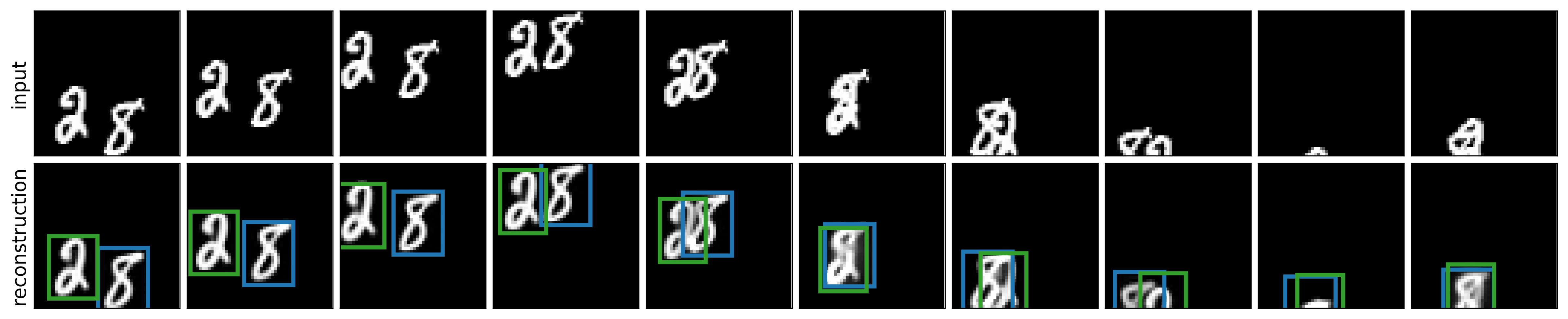
Figure 4: Input images (top) and sqair reconstructions with marked glimpse locations (bottom). For more examples, see Figure 13 in Appendix H.

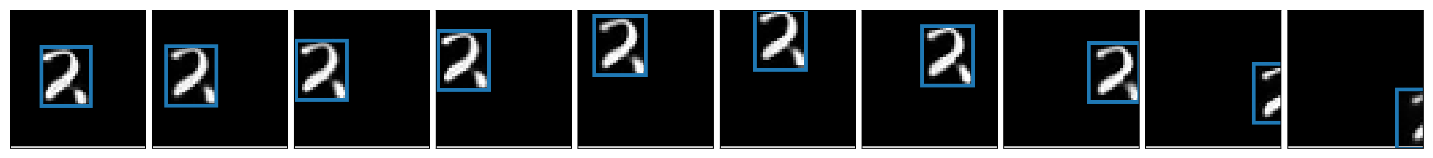
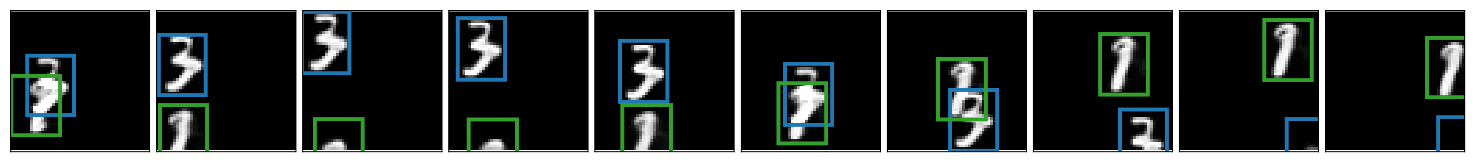
Figure 5: Samples from sqair. Both motion and appearance are consistent through time, thanks to the propagation part of the model. For more examples, see Figure 15 in Appendix H.

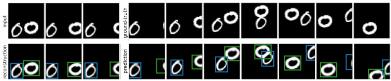
Figure 6: The first three frames are input to sqair, which generated the rest conditional on the first frames.

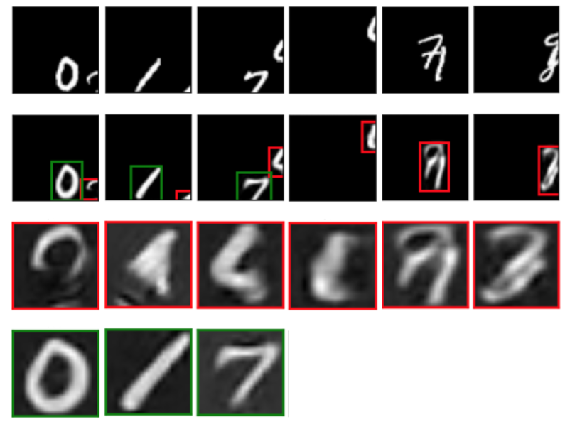
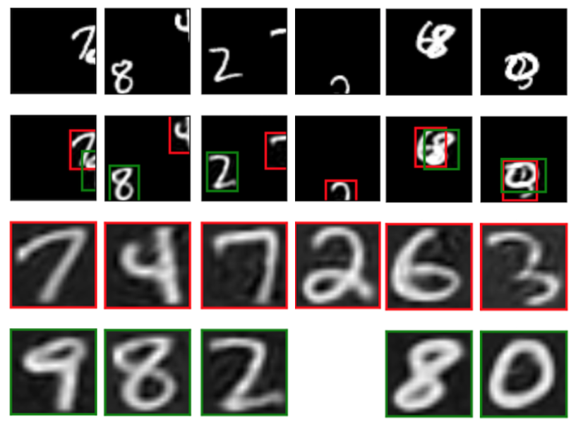
Figure 7: Inputs, reconstructions with marked glimpse locations and reconstructed glimpses for air (left) and sqair (right). Sqair can model partially visible and heavily overlapping objects by aggregating temporal information.

The dataset consists of sequences of length 10 of multiple moving mnist digits. All images are of size $50\times 50$ and there are zero, one or two digits in every frame (with equal probability). Sequences are generated such that no objects overlap in the first frame, and all objects are present through the sequence; the digits can move out of the frame, but always come back. See Appendix F for an experiment on a harder version of this dataset. There are 60,000 training and 10,000 testing sequences created from the respective mnist datasets. We train two variants of sqair: the mlp-sqair uses only fully-connected networks, while the conv-sqair replaces the networks used to encode images and glimpses with convolutional ones; it also uses a subpixel-convolution network as the glimpse decoder [38]. See Appendix D for details of the model architectures and the training procedure.

We use air and vrnn [5] as baselines for comparison. vrnn can be thought of as a sequential vae with an rnn as its deterministic backbone. Being similar to a vae, its latent variables are not structured, nor easily interpretable. For a fair comparison, we control the latent dimensionality of vrnn and the number of learnable parameters. We provide implementation details in Section D.3.

	$\log p_{\theta}\left(\mathbf{x}_{1:T}\right)$	$\log p_{\theta}\left(\mathbf{x}_{1:T}\mid\mathbf{z}_{1:T}\right)$	$\operatorname{KL}\left(q_{\phi}\mid\mid p_{\theta}\right)$	Counting	Addition
conv-sqair	$\bm{6784.8}$	$\bm{6923.8}$	$\bm{134.6}$	$0.9974$	$0.9990$
mlp-sqair	$6617.6$	$6786.5$	$164.5$	$\mathbf{0.9986}$	$\mathbf{0.9998}$
mlp-air	$6443.6$	$6830.6$	$352.6$	$0.9058$	$0.8644$
conv-vrnn	$6561.9$	$6737.8$	$270.2$	n/a	$0.8536$
mlp-vrnn	$5959.3$	$6108.7$	$218.3$	n/a	0.8059

Table 1: sqair achieves higher performance than the baselines across a range of metrics. The third column refers to the kl divergence between the approximate posterior and the prior. Counting refers to accuracy of the inferred number of objects present in the scene, while addition stands for the accuracy of a supervised digit addition experiment, where a classifier is trained on the learned latent representations of each frame.

The quantitative analysis consists of comparing all models in terms of the marginal log-likelihood $\log p_{\theta}\left(\mathbf{x}_{1:T}\right)$ evaluated as the $\mathcal{L}_{\textsc{IWAE}}$ bound with $K=1000$ particles, reconstruction quality evaluated as a single-sample approximation of $\mathbb{E}_{q_{\phi}}\left[\log p_{\theta}\left(\mathbf{x}_{1:T}\mid\mathbf{z}_{1:T}\right)\right]$ and the kl-divergence between the approximate posterior and the prior (Table 1). Additionally, we measure the accuracy of the number of objects modelled by sqair and air. Sqair achieves superior performance across a range of metrics — its convolutional variant outperforms both air and the corresponding vrnn in terms of model evidence and reconstruction performance. The kl divergence for sqair is almost twice as low as for vrnn and by a yet larger factor for air. We can interpret kl values as an indicator of the ability to compress, and we can treat sqair/air type of scheme as a version of run-length encoding. While vrnn has to use information to explicitly describe every part of the image, even if some parts are empty, sqair can explicitly allocate content information ($\mathbf{z}^{\mathrm{what}}$) to specific parts of the image (indicated by $\mathbf{z}^{\mathrm{where}}$). Air exhibits the highest values of kl, but this is due to encoding every frame of the sequence independently — its prior cannot take what and where at the previous time-step into account, hence higher KL. The fifth column of Table 1 details the object counting accuracy, that is indicative of the quality of the approximate posterior. It is measured as the sum of $z_{t}^{\mathrm{pres}}$ for a given frame against the true number of objects in that frame. As there is no $z^{\mathrm{pres}}$ for vrnn no score is provided. Perhaps surprisingly, this metric is much higher for sqair than for air. This is because air mistakenly infers overlapping objects as a single object. Since sqair can incorporate temporal information, it does not exhibit this failure mode (cf. Figure 7). Next, we gauge the utility of the learnt representations by using them to determine the sum of the digits present in the image (Table 1, column six). To do so, we train a 19-way classifier (mapping from any combination of up to two digits in the range $[0,9]$ to their sum) on the extracted representations and use the summed labels of digits present in the frame as the target. Appendix D contains details of the experiment. Sqair significantly outperforms air and both variants of vrnn on this tasks. Vrnn under-performs due to the inability of disentangling overlapping objects, while both vrnn and air suffer from low temporal consistency of learned representations, see Appendix H. Finally, we evaluate sqair qualitatively by analyzing reconstructions and samples produced by the model against reconstructions and samples from vrnn. We observe that samples and reconstructions from sqair are of better quality and, unlike vrnn, preserve motion and appearance consistently through time. See Appendix H for direct comparison and additional examples. Furthermore, we examine conditional generation, where we look at samples from the generative model of sqair conditioned on three images from a real sequence (see Figure 6). We see that the model can preserve appearance over time, and that the simulated objects follow similar trajectories, which hints at good learning of the motion model (see Appendix H for more examples). Figure 7 shows reconstructions and corresponding glimpses of air and sqair. Unlike sqair, air is unable to recognize objects from partial observations, nor can it distinguish strongly overlapping objects (it treats them as a single object; columns five and six in the figure). We analyze failure cases of sqair in Appendix G.

4.2 Generative Modelling of Walking Pedestrians

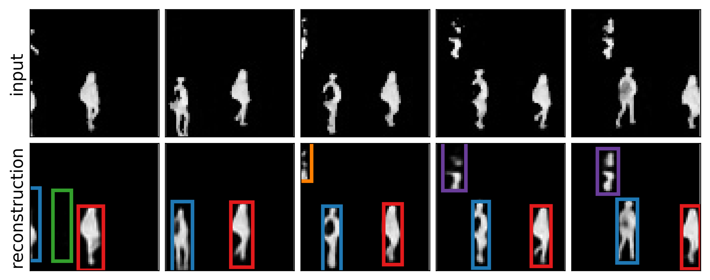
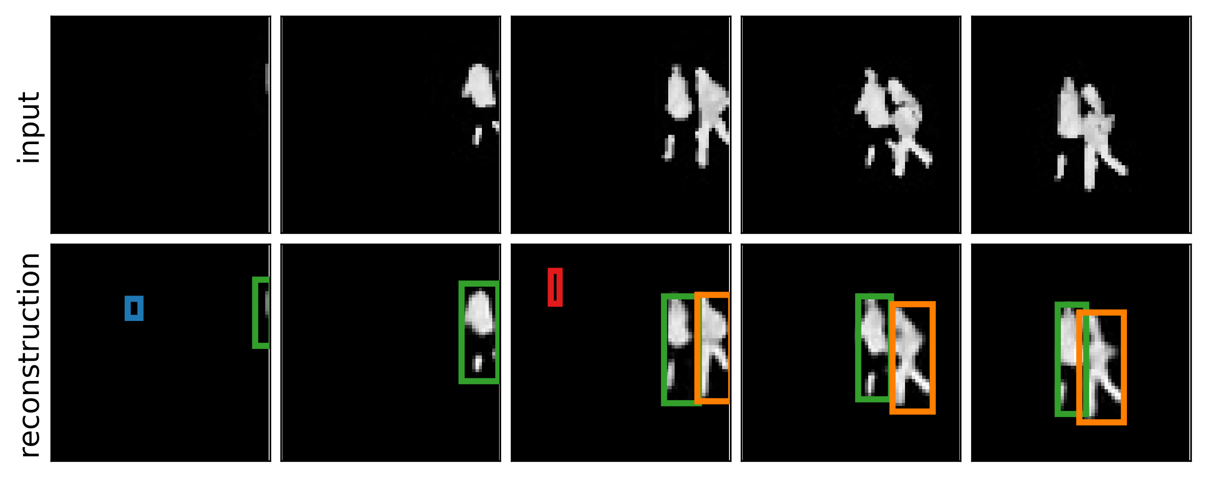
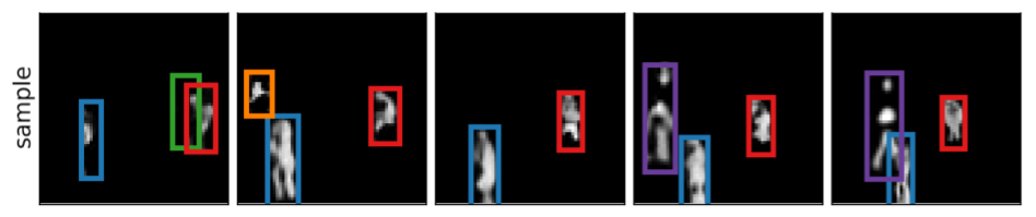
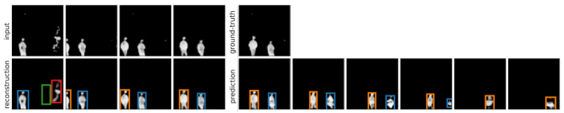
Figure 8: Inputs on the top, reconstructions in the second row, samples in the third row; rows four and five contain inputs and conditional generation: the first four frames in the last row are reconstructions, while the remaining ones are predicted by sampling from the prior. There is no ground-truth, since we used sequences of length five of training and validation.

To evaluate the model in a more challenging, real-world setting, we turn to data from static CCTV cameras of the DukeMTMC dataset [35]. As part of pre-precessing, we use standard background subtraction algorithms [18]. In this experiment, we use $3150$ training and $350$ validation sequences of length $5$. For details of model architectures, training and data pre-processing, see Appendix E. We evaluate the model qualitatively by examining reconstructions, conditional samples (conditioned on the first four frames) and samples from the prior (Figure 8 and Appendix I). We see that the model learns to reliably detect and track walking pedestrians, even when they are close to each other.

There are some spurious detections and re-detections of the same objects, which is mostly caused by imperfections of the background subtraction pipeline — backgrounds are often noisy and there are sudden appearance changes when a part of a person is treated as background in the pre-processing pipeline. The object counting accuracy in this experiment is $0.5712$ on the validation dataset, and we noticed that it does increase with the size of the training set. We also had to use early stopping to prevent overfitting, and the model was trained for only $315$k iterations ($>1$M for mnist experiments). Hence, we conjecture that accuracy and marginal likelihood can be further improved by using a bigger dataset.

5 Related Work

Object Tracking

There have been many approaches to modelling objects in images and videos. Object detection and tracking are typically learned in a supervised manner, where object bounding boxes and often additional labels are part of the training data. Single-object tracking commonly use Siamese networks, which can be seen as an rnn unrolled over two time-steps [43]. Recently, [25] used an rnn with an attention mechanism in the hart model to predict bounding boxes for single objects, while robustly modelling their motion and appearance. Multi-object tracking is typically attained by detecting objects and performing data association on bounding-boxes [2]. [37] used an end-to-end supervised approach that detects objects and performs data association. In the unsupervised setting, where the training data consists of only images or videos, the dominant approach is to distill the inductive bias of spatial consistency into a discriminative model. [4] detect single objects and their parts in images, and [26, 45] incorporate temporal consistency to better track single objects. Sqair is unsupervised and hence it does not rely on bounding boxes nor additional labels for training, while being able to learn arbitrary motion and appearance models similarly to hart [25]. At the same time, is inherently multi-object and performs data association implicitly (cf. Appendix A). Unlike the other unsupervised approaches, temporal consistency is baked into the model structure of sqair and further enforced by lower kl divergence when an object is tracked.

Video Prediction

Many works on video prediction learn a deterministic model conditioned on the current frame to predict the future ones [34, 39]. Since these models do not model uncertainty in the prediction, they can suffer from the multiple futures problem — since perfect prediction is impossible, the model produces blurry predictions which are a mean of possible outcomes. This is addressed in stochastic latent variable models trained using variational inference to generate multiple plausible videos given a sequence of images [1, 8]. Unlike sqair, these approaches do not model objects or their positions explicitly, thus the representations they learn are of limited interpretability.

Learning Decomposed Representations of Images and Videos

Learning decomposed representations of object appearance and position lies at the heart of our model. This problem can be also seen as perceptual grouping, which involves modelling pixels as spatial mixtures of entities. [12] and [13] learn to decompose images into separate entities by iterative refinement of spatial clusters using either learned updates or the Expectation Maximization algorithm; [17] and [40] extend these approaches to videos, achieving very similar results to sqair. Perhaps the most similar work to ours is the concurrently developed model of [16]. The above approaches rely on iterative inference procedures, but do not exhibit the object-counting behaviour of sqair. For this reason, their computational complexities are proportional to the predefined maximum number of objects, while sqair can be more computationally efficient by adapting to the number of objects currently present in an image.

Another interesting line of work is the gan-based unsupervised video generation that decomposes motion and content [42, 7]. These methods learn interpretable features of content and motion, but deal only with single objects and do not explicitly model their locations. Nonetheless, adversarial approaches to learning structured probabilistic models of objects offer a plausible alternative direction of research.

Bayesian Nonparametric Models

To the best of our knowledge, [32] is the only known approach that models pixels belonging to a variable number of objects in a video together with their locations in the generative sense. This work uses a Bayesian nonparametric (BNP) model, which relies on mixtures of Dirichlet processes to cluster pixels belonging to an object. However, the choice of the model necessitates complex inference algorithms involving Gibbs sampling and Sequential Monte Carlo, to the extent that any sensible approximation of the marginal likelihood is infeasible. It also uses a fixed likelihood function, while ours is learnable.

The object appearance-persistence-disappearance model in sqair is reminiscent of the Markov Indian buffet process (MIBP) of [10], another BNP model. MIBP was used as a model for blind source separation, where multiple sources contribute toward an audio signal, and can appear, persist, disappear and reappear independently. The prior in sqair is similar, but the crucial differences are that sqair combines the BNP prior with flexible neural network models for the dynamics and likelihood, as well as variational learning via amortized inference. The interface between deep learning and BNP, and graphical models in general, remains a fertile area of research.

6 Discussion

In this paper we proposed sqair, a probabilistic model that extends air to image sequences, and thereby achieves temporally consistent reconstructions and samples. In doing so, we enhanced air’s capability of disentangling overlapping objects and identifying partially observed objects.

This work continues the thread of [13], [40] and, together with [16], presents unsupervised object detection & tracking with learnable likelihoods by the means of generative modelling of objects. In particular, our work is the first one to explicitly model object presence, appearance and location through time. Being a generative model, sqair can be used for conditional generation, where it can extrapolate sequences into the future. As such, it would be interesting to use it in a reinforcement learning setting in conjunction with Imagination-Augmented Agents [44] or more generally as a world model [15], especially for settings with simple backgrounds, e. g., games like Montezuma’s Revenge or Pacman.

The framework offers various avenues of further research; Sqair leads to interpretable representations, but the interpretability of what variables can be further enhanced by using alternative objectives that disentangle factors of variation in the objects [22]. Moreover, in its current state, sqair can work only with simple backgrounds and static cameras. In future work, we would like to address this shortcoming, as well as speed up the sequential inference process whose complexity is linear in the number of objects. The generative model, which currently assumes additive image composition, can be further improved by e. g., autoregressive modelling [33]. It can lead to higher fidelity of the model and improved handling of occluded objects. Finally, the sqair model is very complex, and it would be useful to perform a series of ablation studies to further investigate the roles of different components.

Appendix A Algorithms

Image generation, described by Algorithm 1, is exactly the same for sqair and air. Algorithms 2 and 3 describe inference in sqair. Note that disc is equivalent to air if no latent variables are present in the inputs.

If a function has multiple inputs and if not stated otherwise, all the inputs are concatenated and linearly projected into some fixed-dimensional space, e. g., Algorithms 2 and 2 in Algorithm 2. Spatial Transformer ($\operatorname{ST}$, e. g., Algorithm 2 in Algorithm 2) has no learnable parameters: it samples a uniform grid of points from an image $\mathbf{x}$, where the grid is transformed according to parameters $\mathbf{z}^{\mathrm{where}}$. $\operatorname{f_{\phi}^{1}}$ is implemented as a perceptron with a single hidden layer. Statistics of $q^{P}$ and $q^{D}$ are a result of applying a two-layer multilayer perceptron (mlp) to their respective conditioning sets. Different distributions $q$ do not share parameters of their mlps. The glimpse encoder $\operatorname{h_{\phi}^{\mathrm{glimpse}}}$ (Algorithms 2 and 2 in Algorithm 2 and Algorithm 3 in Algorithm 3; they share parameters) and the image encoder $\operatorname{h_{\phi}^{\mathrm{enc}}}$ (Algorithm 3 in Algorithm 3) are implemented as two-layer mlps or convolutional neural networks (cnns), depending on the experiment (see Appendices D and E for details).

One of the important details of prop is the proposal glimpse extracted in lines Algorithms 2 and 2 of Algorithm 2. It has a dual purpose. Firstly, it acts as an information bottleneck in prop, limiting the flow of information from the current observation $\mathbf{x}_{t}$ to the updated latent variables $\mathbf{z}_{t}$. Secondly, even though the information is limited, it can still provide a high-resolution view of the object corresponding to the currently updated latent variable, given that the location of the proposal glimpse correctly predicts motion of this object. Initially, our implementation used encoding of the raw observation ($\operatorname{h_{\phi}^{\mathrm{enc}}}\left(\mathbf{x}_{t}\right)$, similarly to Algorithm 3 in Algorithm 3) as an input to the relation-rnn (Algorithm 2 in Algorithm 2). We have also experimented with other bottlenecks: (1) low resolution image as an input to the image encoder and (2) a low-dimensional projection of the image encoding before the relation-rnn. Both approaches have led to ID swaps, where the order of explaining objects were sometimes swapped for different frames of the sequence (see Figure 10 in Appendix G for an example). Using encoded proposal glimpse extracted from a predicted location has solved this issue.

To condition disc on propagated latent variables (Algorithm 3 in Algorithm 3), we encode the latter by using a two-layer mlp similarly to [46],

$$\mathbf{l}_{t}=\sum_{i\in\mathcal{P}_{t}}\operatorname{MLP}\left(\mathbf{z}_{t}^{\mathrm{what},i},\mathbf{z}_{t}^{\mathrm{where},i}\right).$$ (6)

Note that other encoding schemes are possible, though we have experimented only with this one.

Input :  $\mathbf{z}_{t}^{\mathrm{what}},\mathbf{z}_{t}^{\mathrm{where}}$ - latent variables from the current time-step.

$\mathcal{O}_{t}=\operatorname{indices}\left(\mathbf{z}_{t}^{\mathrm{what}}\right)$

 // Indices of all present latent variables.

1 $\mathbf{y}_{t}^{0}=\bm{0}$

2 for $i\in\mathcal{O}_{t}$ do

       $\mathbf{y}_{t}^{\mathrm{att},i}=\operatorname{f_{\theta}^{\mathrm{dec}}}\left(\mathbf{z}_{t}^{\mathrm{what},i}\right)$

       // Decode the glimpse.

3       $\mathbf{y}_{t}^{i}=\mathbf{y}_{t}^{i-1}+\operatorname{ST}^{-1}\left(\mathbf{y}_{t}^{\mathrm{att},i},\mathbf{z}_{t}^{\mathrm{where},i}\right)$

4$\hat{\mathbf{x}}_{t}\sim\mathcal{N}\left(\bm{x}\mid\bm{y}_{n},\sigma^{2}_{x}\bm{I}\right)$

Output : $\hat{\bm{x}}$

Algorithm 1 Image Generation

Input : $\bm{x_{t}}$ - image at the current time-step,

$\mathbf{z}^{\mathrm{what}}_{t-1},\mathbf{z}^{\mathrm{where}}_{t-1},\mathbf{z}^{\mathrm{pres}}_{t-1}$ - latent variables from the previous time-step

$\bm{h}^{T}_{t-1}$ - hidden states from the previous time-step.

1 ${\color[rgb]{1,0.6015625,0}\bm{h}_{t}^{R,0}},\bm{z}^{\mathrm{what},0}_{t},\bm{z}^{\mathrm{where},0}_{t}=\operatorname{initialize}()$

$j=0$

 // Index of the object processed in the last iteration.

2 for $i\in{\mathcal{O}_{t-1}}$ do

3       if $z_{t-1}^{\mathrm{pres},i}==0$ then

4             continue

       $\hat{\mathbf{z}}_{t}^{\mathrm{where},i}=\operatorname{f_{\phi}^{1}}\left(\mathbf{z}_{t-1}^{\mathrm{where},i},{\color[rgb]{0,0,1}\bm{h}_{t}^{T,i}}\right)$

       // Proposal location.

       $\hat{\mathbf{g}}^{i}_{t}=\operatorname{ST}\left(\mathbf{x}_{t},\hat{\mathbf{z}}_{t}^{\mathrm{where},i}\right)$

       // Extract a glimpse from a proposal location.

       $\hat{\mathbf{e}}_{t}^{i}=\operatorname{h_{\phi}^{\mathrm{glimpse}}}\left(\hat{\mathbf{g}}^{i}_{t}\right)$

       // Encode the proposal glimpse.

       ${\color[rgb]{1,0.6015625,0}\mathbf{w}_{t}^{R,i}},{\color[rgb]{1,0.6015625,0}\bm{h}_{t}^{R,i}}={\color[rgb]{1,0.6015625,0}\operatorname{R}_{\phi}^{R}}\left(\hat{\mathbf{e}}_{t}^{i},\mathbf{z}_{t-1}^{\mathrm{what},i},\mathbf{z}_{t-1}^{\mathrm{where},i},{\color[rgb]{0,0,1}\bm{h}_{t-1}^{T,i}},{\color[rgb]{1,0.6015625,0}\bm{h}_{t}^{R,j}},\mathbf{z}_{t}^{\mathrm{what},j},\mathbf{z}_{t}^{\mathrm{where},j}\right)$

       // Relational state, see Equation 14.

5       $\mathbf{z}_{t}^{\mathrm{where},i}\sim q^{P}_{\phi}\left(\bm{z}^{\mathrm{where}}\mid\bm{z}^{\mathrm{where},k}_{t-1},{\color[rgb]{1,0.6015625,0}\mathbf{w}_{t}^{R,i}}\right)$

       $\mathbf{g}_{t}^{i}=\operatorname{ST}\left(\mathbf{x}_{t},\mathbf{z}_{t}^{\mathrm{where},i}\right)$

       // Extract the final glimpse.

       $\mathbf{e}_{t}^{i}=\operatorname{h_{\phi}^{\mathrm{glimpse}}}\left(\mathbf{g}_{t}^{i}\right)$

       // Encode the final glimpse.

       ${\color[rgb]{0,0,1}\mathbf{w}_{t}^{T,i}},{\color[rgb]{0,0,1}\bm{h}_{t}^{T,i}}={\color[rgb]{0,0,1}\operatorname{R}_{\phi}^{T}}\left(\mathbf{e}_{t}^{i},\mathbf{z}_{t}^{\mathrm{where},i},{\color[rgb]{0,0,1}\bm{h}_{t-1}^{T,i}},{\color[rgb]{1,0.6015625,0}\bm{h}_{t}^{R,i}}\right)$

       // Temporal state, see Equation 15.

6       $\mathbf{z}_{t}^{\mathrm{what},i}\sim q^{P}_{\phi}\left(\mathbf{z}^{\mathrm{what}}\mid\mathbf{e}_{t}^{i},\mathbf{z}_{t-1}^{\mathrm{what},i},{\color[rgb]{1,0.6015625,0}\mathbf{w}_{t}^{R,i}},{\color[rgb]{0,0,1}\mathbf{w}_{t}^{T,i}}\right)$

       $z_{t}^{\mathrm{pres},i}\sim q^{P}_{\phi}\left(z^{\mathrm{pres}}\mid z_{t-1}^{\mathrm{pres},i},\mathbf{z}_{t}^{\mathrm{what},i},\mathbf{z}_{t}^{\mathrm{where},i},{\color[rgb]{1,0.6015625,0}\mathbf{w}_{t}^{R,i}},{\color[rgb]{0,0,1}\mathbf{w}_{t}^{T,i}}\right)$

       // Equation 13.

7       $j=i$

Output :  $\mathbf{z}_{t}^{\mathrm{what},\mathcal{P}_{t}},\mathbf{z}_{t}^{\mathrm{where},\mathcal{P}_{t}},\mathbf{z}_{t}^{\mathrm{pres},\mathcal{P}_{t}}$

Algorithm 2 Inference for Propagation

Input :  $\bm{x_{t}}$ - image at the current time-step,

$\mathbf{z}_{t}^{\mathcal{P}_{t}}$ - propagated latent variables for the current time-step,

$N$ - maximum number of inference steps for discovery.

1 ${\color[rgb]{1,0,1}\bm{h}_{t}^{D,0}},\bm{z}^{\mathrm{what},0}_{t},\bm{z}^{\mathrm{where},0}_{t}=\operatorname{initialize}()$

$j=\operatorname{max\_index}\left(\mathbf{z}_{t}^{\mathcal{P}_{t}}\right)$

 // Maximum index among the propagated latent variables.

$\mathbf{e}_{t}=\operatorname{h_{\phi}^{\mathrm{enc}}}\left(\mathbf{x}_{t}\right)$

 // Encode the image.

$\mathbf{l}_{t}=\operatorname{h_{\phi}^{\mathrm{enc}}}\left(\mathbf{z}_{t}^{\mathrm{what}},\mathbf{z}_{t}^{\mathrm{where}},\mathbf{z}_{t}^{\mathrm{pres}}\right)$

 // Encode latent variables.

2 for $i\in[j+1,\dots,j+N]$ do

3       ${\color[rgb]{1,0,1}\mathbf{w}_{t}^{D,i}},{\color[rgb]{1,0,1}\bm{h}_{t}^{D,i}}={\color[rgb]{1,0,1}\operatorname{R}_{\phi}^{D}}\left(\mathbf{e}_{t},\mathbf{l}_{t},\mathbf{z}_{t}^{\mathrm{what},i-1},\mathbf{z}_{t}^{\mathrm{where},i-1},{\color[rgb]{1,0,1}\bm{h}_{t}^{D,i-1}}\right)$

4       $z_{t}^{\mathrm{pres},i}\sim q^{D}_{\phi}\left(z^{\mathrm{pres}}\mid{\color[rgb]{1,0,1}\mathbf{w}_{t}^{D,i}}\right)$

5       if $z^{\mathrm{pres},i}=0$ then

6             break

7      $\mathbf{z}_{t}^{\mathrm{where},i}\sim q^{D}_{\phi}\left(\mathbf{z}^{\mathrm{where}}\mid{\color[rgb]{1,0,1}\mathbf{w}_{t}^{D,i}}\right)$

8       $\mathbf{g}_{t}^{i}=\operatorname{ST}\left(\mathbf{x}_{t},\mathbf{z}_{t}^{\mathrm{where},i}\right)$

       $\mathbf{e}_{t}^{i}=\operatorname{h_{\phi}^{\mathrm{glimpse}}}\left(\mathbf{g}_{t}^{i}\right)$

       // Encode the glimpse.

9       $\mathbf{z}_{t}^{\mathrm{what},i}\sim q^{D}_{\phi}\left(\mathbf{z}_{t}^{\mathrm{what}}\mid\mathbf{e}_{t}^{i}\right)$

Output :  $\mathbf{z}_{t}^{\mathrm{what},\mathcal{D}_{t}},\mathbf{z}_{t}^{\mathrm{where},\mathcal{D}_{t}},\mathbf{z}_{t}^{\mathrm{pres},\mathcal{D}_{t}}$

Algorithm 3 Inference for Discovery

Appendix B Details for the Generative Model of SQAIR

In implementation, we upper bound the number of objects at any given time by $N$. In detail, the discovery prior is given by

$$p^{D}\left(D_{t},\mathbf{z}_{t}^{\mathcal{D}_{t}}\mid\mathbf{z}_{t}^{\mathcal{P}_{t}}\right)=p^{D}\left(D_{t}\mid P_{t}\right)\prod_{i\in\mathcal{D}_{t}}p^{D}(\mathbf{z}_{t}^{\mathrm{what},i})p^{D}(\mathbf{z}_{t}^{\mathrm{where},i})\delta_{1}(z_{t}^{\mathrm{pres},i}),$$ (7)

$$p^{D}\left(D_{t}\mid P_{t}\right)=\operatorname{Categorical}\left(D_{t};N-P_{t},p_{\theta}(P_{t})\right),$$ (8)

where $\delta_{x}(\cdot)$ is the delta function at $x$, $\operatorname{Categorical}(k;K,p)$ implies $k\in\{0,1,\ldots,K\}$ with probabilities $p_{0},p_{1},\ldots,p_{K}$ and $p^{D}(\mathbf{z}_{t}^{\mathrm{what},i}),p^{D}(\mathbf{z}_{t}^{\mathrm{where},i})$ are fixed isotropic Gaussians. The propagation prior is given by

$$p^{P}\left(\mathbf{z}_{t}^{\mathcal{P}_{t}}\mid\mathbf{z}_{t-1}\right)=\prod_{i\in\mathcal{P}_{t}}p^{P}\left(\mathbf{z}_{t}^{\mathrm{pres},i}\mid\mathbf{z}_{t-1}^{\mathrm{pres},i},\bm{h}_{t-1}\right)p^{P}\left(\mathbf{z}_{t}^{\mathrm{what},i}\mid\bm{h}_{t-1}\right)p^{P}\left(\mathbf{z}_{t}^{\mathrm{where},i}\mid\bm{h}_{t-1}\right),$$ (9)

$$p^{P}\left(\mathbf{z}_{t}^{\mathrm{pres},i}\mid\mathbf{z}_{t-1}^{\mathrm{pres},i},\bm{h}_{t-1}\right)=\operatorname{Bernoulli}(z_{t}^{\mathrm{pres},i};f_{\theta}(\bm{h}_{t-1}))\delta_{1}(z_{t-1}^{\mathrm{pres},i}),$$ (10)

with $f_{\theta}$ a scalar-valued function with range $[0,1]$ and $p^{P}(\mathbf{z}_{t}^{\mathrm{what},i}|\bm{h}_{t-1})$, $p^{P}(\mathbf{z}_{t}^{\mathrm{where},i}|\bm{h}_{t-1})$ both factorised Gaussians parameterised by some function of $\bm{h}_{t-1}$.

Appendix C Details for the Inference of SQAIR

The propagation inference network $q^{P}_{\phi}$ is given as below,

$$q^{P}_{\phi}\left(\mathbf{z}_{t}^{\mathcal{P}_{t}}\mid\mathbf{x}_{t},\mathbf{z}_{t-1},{\color[rgb]{0,0,1}\bm{h}_{t}^{T,\mathcal{P}_{t}}}\right)=\prod_{i\in{\mathcal{O}_{t-1}}}q^{P}_{\phi}\left(\mathbf{z}_{t}^{i}\mid\mathbf{x}_{t},\mathbf{z}_{t-1}^{i},{\color[rgb]{0,0,1}\bm{h}_{t}^{T,i}},{\color[rgb]{1,0.6015625,0}\bm{h}_{t}^{R,i}}\right),$$ (11)

with ${\color[rgb]{1,0.6015625,0}\bm{h}_{t}^{R,i}}$ the hidden state of the relation rnn (see Equation 14). Its role is to capture information from the observation $\mathbf{x}_{t}$ as well as to model dependencies between different objects. The propagation posterior for a single object can be expanded as follows,

$$q^{P}_{\phi}\left(\mathbf{z}_{t}^{i}\mid\mathbf{x}_{t},\mathbf{z}_{t-1}^{i},{\color[rgb]{0,0,1}\bm{h}_{t}^{T,i}},{\color[rgb]{1,0.6015625,0}\bm{h}_{t}^{R,i}}\right)=$$ (12)

$$\quad q^{P}_{\phi}\left(\mathbf{z}_{t}^{\mathrm{where},i}\mid\mathbf{z}_{t-1}^{\mathrm{what},i},\mathbf{z}_{t-1}^{\mathrm{where},i},{\color[rgb]{0,0,1}\bm{h}_{t-1}^{T,i}},{\color[rgb]{1,0.6015625,0}\bm{h}_{t}^{R,i}}\right)$$

$$\quad q^{P}_{\phi}\left(\mathbf{z}_{t}^{\mathrm{what},i}\mid\mathbf{x}_{t},\mathbf{z}_{t}^{\mathrm{where},i},\mathbf{z}_{t-1}^{\mathrm{what},i},{\color[rgb]{0,0,1}\bm{h}_{t}^{T,i}},{\color[rgb]{1,0.6015625,0}\bm{h}_{t}^{R,i}}\right)$$

$$\quad q^{P}_{\phi}\left(z_{t}^{\mathrm{pres},i}\mid\mathbf{z}_{t}^{\mathrm{what},i},\mathbf{z}_{t}^{\mathrm{where},i},z_{t-1}^{\mathrm{pres},i},{\color[rgb]{0,0,1}\bm{h}_{t}^{T,i}},{\color[rgb]{1,0.6015625,0}\bm{h}_{t}^{R,i}}\right).$$

In the second line, we condition the object location $\mathbf{z}_{t}^{\mathrm{where},i}$ on its previous appearance and location as well as its dynamics and relation with other objects. In the third line, current appearance $\mathbf{z}_{t}^{\mathrm{what},i}$ is conditioned on the new location. Both $\mathbf{z}_{t}^{\mathrm{where},i}$ and $\mathbf{z}_{t}^{\mathrm{what},i}$ are modelled as factorised Gaussians. Finally, presence depends on the new appearance and location as well as the presence of the same object at the previous time-step. More specifically,

$$q^{P}_{\phi}\left(z_{t}^{\mathrm{pres},i}\mid\mathbf{z}_{t}^{\mathrm{what},i},\mathbf{z}_{t}^{\mathrm{where},i},z_{t-1}^{\mathrm{pres},i},{\color[rgb]{0,0,1}\bm{h}_{t}^{T,i}},{\color[rgb]{1,0.6015625,0}\bm{h}_{t}^{R,i}}\right)$$ (13)

$$\quad=\operatorname{Bernoulli}\left(z_{t}^{\mathrm{pres},i}\mid f_{\phi}\left(\mathbf{z}_{t}^{\mathrm{what},i},\mathbf{z}_{t}^{\mathrm{where},i},{\color[rgb]{0,0,1}\bm{h}_{t}^{T,i}},{\color[rgb]{1,0.6015625,0}\bm{h}_{t}^{R,i}}\right)\right)\delta_{1}(z_{t-1}^{\mathrm{pres},i}),$$

where the second term is the delta distribution centered on the presence of this object at the previous time-step. If it was not there, it cannot be propagated. Let $j\in\{0,\dots,i-1\}$ be the index of the most recent present object before object $i$. Hidden states are updated as follows,

$${\color[rgb]{1,0.6015625,0}\bm{h}_{t}^{R,i}}={\color[rgb]{1,0.6015625,0}\operatorname{R}_{\phi}^{R}}\left(\mathbf{x}_{t},\mathbf{z}_{t-1}^{\mathrm{what},i},\mathbf{z}_{t-1}^{\mathrm{where},i},{\color[rgb]{0,0,1}\bm{h}_{t-1}^{T,i}},{\color[rgb]{1,0.6015625,0}\bm{h}_{t}^{R,i-1}},\mathbf{z}_{t}^{\mathrm{what},j},\mathbf{z}_{t}^{\mathrm{where},j}\right),$$ (14)

$${\color[rgb]{0,0,1}\bm{h}_{t}^{T,i}}={\color[rgb]{0,0,1}\operatorname{R}_{\phi}^{T}}\left(\mathbf{x}_{t},\mathbf{z}_{t}^{\mathrm{where},i},{\color[rgb]{0,0,1}\bm{h}_{t-1}^{T,i}},{\color[rgb]{1,0.6015625,0}\bm{h}_{t}^{R,i}}\right),$$ (15)

where ${\color[rgb]{0,0,1}\operatorname{R}_{\phi}^{T}}$ and ${\color[rgb]{1,0.6015625,0}\operatorname{R}_{\phi}^{R}}$ are temporal and propagation RNNs, respectively. Note that in Eq. 14 the rnn does not have direct access to the image $\mathbf{x}_{t}$, but rather accesses it by extracting an attention glimpse at a proposal location, predicted from ${\color[rgb]{0,0,1}\bm{h}_{t-1}^{T,i}}$ and $\mathbf{z}_{t-1}^{\mathrm{where},i}$. This might seem like a minor detail, but in practice structuring computation this way prevents ID swaps from occurring, cf. Appendix G. For computational details, please see Algorithms 2 and 3 in Appendix A.

Appendix D Details of the moving-mnist Experiments

D.1 Sqair and air Training Details

All models are trained by maximising the evidence lower bound (elbo) $\mathcal{L}_{IWAE}$ (Equation 5) with the rmsprop optimizer [41] with momentum equal to $0.9$. We use the learning rate of $10^{-5}$ and decrease it to $\frac{1}{3}\cdot 10^{-5}$ after 400k and to $10^{-6}$ after 1000k training iterations. Models are trained for the maximum of $2\cdot 10^{6}$ training iterations; we apply early stopping in case of overfitting. Sqair models are trained with a curriculum of sequences of increasing length: we start with three time-steps, and increase by one time-step every $10^{5}$ training steps until reaching the maximum length of 10. When training air, we treated all time-steps of a sequence as independent, and we trained it on all data (sequences of length ten, split into ten independent sequences of length one).

D.2 Sqair and air Model Architectures

All models use glimpse size of $20\times 20$ and exponential linear unit (elu) [6] non-linearities for all layers except RNNs and output layers. mlp-sqair uses fully-connected layers for all networks. In both variants of sqair, the ${\color[rgb]{1,0,1}\operatorname{R}_{\phi}^{D}}$ and ${\color[rgb]{1,0.6015625,0}\operatorname{R}_{\phi}^{R}}$ RNNs are the vanilla RNNs. The propagation prior rnn and the temporal rnn ${\color[rgb]{0,0,1}\operatorname{R}_{\phi}^{T}}$ use gated recurrent unit (gru). air follows the same architecture as mlp-sqair. All fully-connected layers and RNNs in mlp-sqair and air have 256 units; they have $2.9$M and $1.7$M trainable parameters, respectively.

Conv-sqair differs from the mlp version in that it uses cnns for the glimpse and image encoders and a subpixel-cnn [38] for the glimpse decoder. All fully connected layers and RNNs have 128 units. The encoders share the cnn, which is followed by a single fully-connected layer (different for each encoder). The cnn has four convolutional layers with $[16,32,32,64]$ features maps and strides of $[2,2,1,1]$. The glimpse decoder is composed of two fully-connected layers with $[256,800]$ hidden units, whose outputs are reshaped into $32$ features maps of size $5\times 5$, followed by a subpixel-cnn with three layers of $[32,64,64]$ feature maps and strides of $[1,2,2]$. All filters are of size $3\times 3$. Conv-sqair has $2.6$M trainable parameters.

We have experimented with different sizes of fully-connected layers and RNNs; we kept the size of all layers the same and altered it in increments of 32 units. Values greater than 256 for mlp-sqair and 128 for conv-sqair resulted in overfitting. Models with as few as 32 units per layer ($<0.9$M trainable parameters for mlp-sqair) displayed the same qualitative behaviour as reported models, but showed lower quantitative performance.

The output likelihood used in both sqair and air is Gaussian with a fixed standard deviation set to $0.3$, as used by [9]. We tried using a learnable scalar standard deviation, but decided not to report it due to unsable behaviour in the early stages of training. Typically, standard deviation would converge to a low value early in training, which leads to high penalties for reconstruction mistakes. In this regime, it is beneficial for the model to perform no inference steps ($z^{\mathrm{pres}}$ is always equal to zero), and the model never learns. Fixing standard deviation for the first $10$k iterations and then learning it solves this issue, but it introduces unnecessary complexity into the training procedure.

D.3 Vrnn Implementation and Training Details

Our vrnn implementation is based on the implementation of Filtering Variational Objectives (fivo) by [29]. We use an lstm with hidden size $J$ for the deterministic backbone of the vrnn. At time $t$, the lstm receives $\psi^{x}(\mathbf{x}_{t-1})$ and $\psi^{z}(\mathbf{z}_{t-1})$ as input and outputs $o_{t}$, where $\psi^{x}$ is a data feature extractor and $\psi^{z}$ is a latent feature extractor. The output is mapped to the mean and standard deviation of the Gaussian prior $p_{\theta}\left(\mathbf{z}_{t}\mid\mathbf{x}_{t-1}\right)$ by an mlp. The likelihood $p_{\theta}\left(\mathbf{x}_{t}\mid\mathbf{z}_{t},\mathbf{x}_{t-1}\right)$ is a Gaussian, with mean given by $\psi^{\mathrm{dec}}(\psi^{z}(\mathbf{z}_{t}),o_{t})$ and standard deviation fixed to be $0.3$ as for sqair and air. The inference network $q_{\phi}\left(\mathbf{z}_{t}\mid\mathbf{z}_{t-1},\mathbf{x}_{t}\right)$ is a Gaussian with mean and standard deviation given by the output of separate mlp s with inputs $[o_{t},\psi^{x}(\mathbf{x}_{t})]$.

All aforementioned mlps use the same number of hidden units $H$ and the same number of hidden layers $L$. The conv-vrnn uses a cnn for $\psi^{x}$ and a transposed cnn for $\psi^{\mathrm{dec}}$. The mlp-vrnn uses an mlp with $H^{\prime}$ hidden units and $L^{\prime}$ hidden layers for both. Elu were used throughout as activations. The latent dimensionality was fixed to 165, which is the upper bound of the number of latent dimensions that can be used per time-step in sqair or air. Training was done by optimising the fivo bound, which is known to be tighter than the iwae bound for sequential latent variable models [29]. We also verified that this was the case with our models on the moving-mnist data. We train with the rmsprop optimizer with a learning rate of $10^{-5}$, momentum equal to $0.9$, and training until convergence of test fivo bound.

For each of mlp-vrnn and conv-vrnn, we experimented with three architectures: small/medium/large. We used $H$=$H^{\prime}$=$J$=128/256/512 and $L$=$L^{\prime}$=2/3/4 for mlp-vrnn, giving number of parameters of $1.2$M/$2.1$M/$9.8$M. For conv-vrnn, the number of features maps we used was $[32,32,64,64]$, $[32,32,32,64,64,64]$ and $[32,32,32,64,64,64,64,64,64]$, with strides of $[2,2,2,2]$, $[1,2,1,2,1,2]$ and $[1,2,1,2,1,2,1,1,1]$, all with $3\times 3$ filters, $H$=$J$=$128$/$256$/$512$ and $L$=1, giving number of parameters of $0.8$M/$2.6$M/$6.1$M. The largest convolutional encoder architecture is very similar to that in [14] applied to mnist.

We have chosen the medium-sized models for comparison with sqair due to overfitting encountered in larger models.

Table 2: Number of trainable parameters for the reported models.

	conv-sqair	mlp-sqair	mlp-air	conv-vrnn	mlp-vrnn
number of parameters	$2.6$M	$2.9$M	$1.7$M	$2.6$M	$2.1$M

D.4 Addition Experiment

We perform the addition experiment by feeding latent representations extracted from the considered models into a 19-way classifier, as there are 19 possible outputs (addition of two digits between 0 and 9). The classifier is implemented as an mlp with two hidden layers with 256 elu units each and a softmax output. For air and sqair, we use concatenated $\mathbf{z}^{\mathrm{what}}$ variables multiplied by the corresponding $z^{\mathrm{pres}}$ variables, while for vrnn we use the whole 165-dimensional latent vector. We train the model over $10^{7}$ training iterations with the adam optimizer [23] with default parameters (in tensorflow).

Appendix E Details of the DukeMTMC Experiments

We take videos from cameras one, two, five, six and eight from the DukeMTMC dataset [35]. As pre-processing, we invert colors and subtract backgrounds using standard OpenCV tools [18], downsample to the resolution of $240\times 175$, convert to gray-scale and randomly crop fragments of size $64\times 64$. Finally, we generate $3500$ sequences of length five such that the maximum number of objects present in any single frame is three and we split them into training and validation sets with the ratio of $9:1$.

We use the same training procedure as for the mnist experiments. The only exception is the learning curriculum, which goes from three to five time-steps, since this is the maximum length of the sequences.

The reported model is similar to conv-sqair. We set the glimpse size to $28\times 12$ to account for the expected aspect ratio of pedestrians. Glimpse and image encoders share a cnn with $[16,32,64,64]$ feature maps and strides of $[2,2,2,1]$ followed by a fully-connected layer (different for each encoder). The glimpse decoder is implemented as a two-layer fully-connected network with 128 and 1344 units, whose outputs are reshaped into 64 feature maps of size $7\times 3$, followed by a subpixel-cnn with two layers of $[64,64]$ feature maps and strides of $[2,2]$. All remaining fully-connected layers in the model have 128 units. The total number of trainable parameters is $3.5$M.

Appendix F Harder multi-mnist Experiment

We created a version of the multi-mnist dataset, where objects can appear or disappear at an arbitrary point in time. It differs from the dataset described in Section 4.1, where all digits are present throughout the sequence. All other dataset parameters are the same as in Section 4.1. Figure 9 shows an example sequence and mlp-sqair reconstructions with marked glimpse locations. The model has no trouble detecting new digits in the middle of the sequence and rediscovering a digit that was previously present.

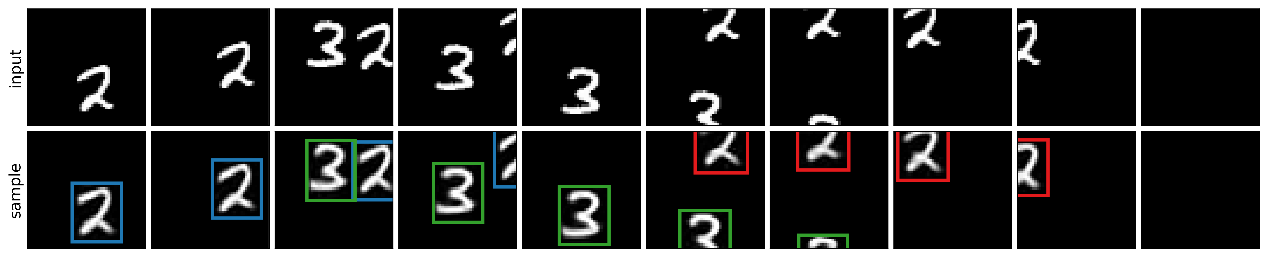
Figure 9: sqair trained on a harder version of moving-textscmnist. Input images (top) and sqair reconstructions with marked glimpse locations (bottom)

Appendix G Failure cases of sqair

Figure 10: Examples of ID swaps in a version of sqair without proposal glimpse extraction in prop (see Appendix A for details). Bounding box colours correspond to object index (or its identity). When prop is allowed the same access to the image as disc, then it often prefers to ignore latent variables, which leads to swapped inference order.

Figure 11: Examples of re-detections in mlp-sqair. Bounding box colours correspond to object identity, assigned to it upon discovery. In some training runs, sqair converges to a solution, where objects are re-detected in the second frame, and prop starts tracking only in the third frame (left). Occasionally, an object can be re-detected after it has severely overlapped with another one (top right). Sometimes the model decides to use only disc and repeatedly discovers all objects (bottom right). These failure mode seem to be mutually exclusive – they come from different training runs.

Figure 12: Two failed reconstructions of sqair. Left: Sqair re-detects objects in the second time-step. Instead of 5 and 2, however, it reconstructs them as 6 and 7. Interestingly, reconstructions are consistent through the rest of the sequence. Right: At the second time-step, overlapping 6 and 8 are explained as 6 and a small 0. The model realizes its mistake in the third time-step, re-detects both digits and reconstructs them properly.

Appendix H Reconstruction and Samples from the Moving-MNIST Dataset

H.1 Reconstructions

Figure 13: Sequences of input (first row) and sqair reconstructions with marked glimpse locations. Reconstructions are all temporally consistent.

Figure 14: Sequences of input (first row) and conv-vrnn reconstructions. They are not temporally consistent. The reconstruction at time $t=1$ is typically of lower quality and often different than the rest of the sequence.

H.2 Samples

Figure 15: Samples from sqair. Both motion and appearance are temporally consistent. In the last sample, the model introduces the third object despite the fact that it has seen only up to two objects in training.

Figure 16: Samples from conv-vrnn. They show lack of temporal consistency. Objects in the generated frames change between consecutive time-steps and they do not resamble digits from the training set.

H.3 Conditional Generation

Figure 17: Conditional generation from sqair, which sees only the first three frames in every case. Top is the input sequence (and the remaining ground-truth), while bottom is reconstruction (first three time-steps) and then generation.

Appendix I Reconstruction and Samples from the DukeMTMC Dataset

Figure 18: Sequences of input (first row) and sqair reconstructions with marked glimpse locations. While not perfect (spurious detections, missed objects), they are temporally consistent and similar in appearance to the inputs.

Figure 19: Samples with marked glimpse locations from sqair trained on the DukeMTMC dataset. Both appearance and motion is spatially consistent. Generated objects are similar in appearance to pedestrians in the training data. Samples are noisy, but so is the dataset.

Figure 20: Conditional generation from sqair, which sees only the first four frames in every case. Top is the input sequence (and the remaining ground-truth), while bottom is reconstruction (first four time-steps) and then generation.

References

- [1] Mohammad Babaeizadeh, Chelsea Finn, Dumitru Erhan, Roy H. Campbell and Sergey Levine “Stochastic Variational Video Prediction” In CoRR, 2017 arXiv:1710.11252
- [2] Alex Bewley, ZongYuan Ge, Lionel Ott, Fabio Tozeto Ramos and Ben Upcroft “Simple online and realtime tracking” In ICIP, 2016, pp. 3464–3468
- [3] Yuri Burda, Roger Grosse and Ruslan Salakhutdinov “Importance Weighted Autoencoders” In ICLR, 2016 arXiv: http://arxiv.org/abs/1509.00519
- [4] Minsu Cho, Suha Kwak, Cordelia Schmid and Jean Ponce “Unsupervised object discovery and localization in the wild: Part-based matching with bottom-up region proposals” In CoRR, 2015 arXiv:1501.06170
- [5] Junyoung Chung, Kyle Kastner, Laurent Dinh, Kratarth Goel, Aaron Courville and Yoshua Bengio “A Recurrent Latent Variable Model for Sequential Data” In NIPS, 2015 arXiv: http://arxiv.org/abs/1506.02216
- [6] Djork-Arné Clevert, Thomas Unterthiner and Sepp Hochreiter “Fast and Accurate Deep Network Learning by Exponential Linear Units (ELUs)” In CoRR, 2015 arXiv:1511.07289
- [7] Emily Denton and Vighnesh Birodkar “Unsupervised learning of disentangled representations from video” In NIPS, 2017, pp. 4417–4426
- [8] Emily Denton and Rob Fergus “Stochastic Video Generation with a Learned Prior” In ICML, 2018
- [9] S.. Eslami, Nicolas Heess, Theophane Weber, Yuval Tassa, David Szepesvari, Koray Kavukcuoglu and Geoffrey E. Hinton “Attend, Infer, Repeat: Fast Scene Understanding with Generative Models” In NIPS, 2016 arXiv: http://arxiv.org/abs/1603.08575
- [10] Jurgen Van Gael, Yee Whye Teh and Zoubin Ghahramani “The Infinite Factorial Hidden Markov Model” In NIPS, 2009, pp. 1697–1704 URL: https://papers.nips.cc/paper/3518-the-infinite-factorial-hidden-markov-model
- [11] Alex Graves, Greg Wayne, Malcolm Reynolds, Tim Harley, Ivo Danihelka, Agnieszka Grabska-Barwińska, Sergio Gómez Colmenarejo, Edward Grefenstette, Tiago Ramalho, John Agapiou, Adrià Puigdomènech Badia, Karl Moritz Hermann, Yori Zwols, Georg Ostrovski, Adam Cain, Helen King, Christopher Summerfield, Phil Blunsom, Koray Kavukcuoglu and Demis Hassabis “Hybrid computing using a neural network with dynamic external memory” In Nature 538.7626 Macmillan Publishers Limited, part of Springer Nature. All rights reserved., 2016, pp. 471–476 URL: http://dx.doi.org/10.1038/nature20101%20http://10.0.4.14/nature20101%20http://www.nature.com/nature/journal/v538/n7626/abs/nature20101.html%7B%5C#%7Dsupplementary-information
- [12] Klaus Greff, Antti Rasmus, Mathias Berglund, Tele Hotloo Hao, Harri Valpola and Jürgen Schmidhuber “Tagger: Deep Unsupervised Perceptual Grouping” In NIPS, 2016
- [13] Klaus Greff, Sjoerd Steenkiste and Jürgen Schmidhuber “Neural Expectation Maximization” In NIPS, 2017
- [14] Ishaan Gulrajani, Kundan Kumar, Faruk Ahmed, Adrien Ali Taiga, Francesco Visin, David Vazquez and Aaron Courville “Pixelvae: A latent variable model for natural images” In CoRR, 2016 arXiv:1611.05013
- [15] David Ha and Jürgen Schmidhuber “World Models” In CoRR, 2018 arXiv:1603.10122
- [16] Jun-Ting Hsieh, Bingbin Liu, De-An Huang, Li Fei-Fei and Juan Carlos Niebles “Learning to Decompose and Disentangle Representations for Video Prediction” In NIPS, 2018
- [17] Alexander Ilin, Isabeau Prémont-Schwarz, Tele Hotloo Hao, Antti Rasmus, Rinu Boney and Harri Valpola “Recurrent Ladder Networks” In NIPS, 2017
- [18] Itseez “Open Source Computer Vision Library”, https://github.com/itseez/opencv, 2015
- [19] Jörn-Henrik Jacobsen, Jan Van Gemert, Zhongyou Lou and Arnold W M Smeulders “Structured Receptive Fields in CNNs” In CVPR, 2016 URL: https://www.cv-foundation.org/openaccess/content%7B%5C_%7Dcvpr%7B%5C_%7D2016/papers/Jacobsen%7B%5C_%7DStructured%7B%5C_%7DReceptive%7B%5C_%7DFields%7B%5C_%7DCVPR%7B%5C_%7D2016%7B%5C_%7Dpaper.pdf
- [20] Max Jaderberg, Karen Simonyan, Andrew Zisserman and Koray Kavukcuoglu “Spatial Transformer Networks” In NIPS, 2015 DOI: 10.1038/nbt.3343
- [21] Charles Kemp and Joshua B Tenenbaum “The discovery of structural form” In Proceedings of the National Academy of Sciences 105.31 National Acad Sciences, 2008, pp. 10687–10692
- [22] Hyunjik Kim and Andriy Mnih “Disentangling by factorising” In ICML, 2018 arXiv:1802.05983
- [23] Diederik P. Kingma and Jimmy Ba “Adam: A Method for Stochastic Optimization” In ICLR, 2015 arXiv:1412.6980
- [24] Diederik P Kingma and Max Welling “Auto-encoding variational bayes” In arXiv preprint arXiv:1312.6114, 2013
- [25] Adam R. Kosiorek, Alex Bewley and Ingmar Posner “Hierarchical Attentive Recurrent Tracking” In NIPS, 2017 arXiv: http://arxiv.org/abs/1706.09262
- [26] Suha Kwak, Minsu Cho, Ivan Laptev, Jean Ponce and Cordelia Schmid “Unsupervised object discovery and tracking in video collections” In ICCV, 2015, pp. 3173–3181 IEEE
- [27] Yann LeCun, Yoshua Bengio and Geoffrey Hinton “Deep learning” In Nature 521.7553 Nature Publishing Group, 2015, pp. 436
- [28] Yann LeCun, Bernhard Boser, John S Denker, Donnie Henderson, Richard E Howard, Wayne Hubbard and Lawrence D Jackel “Backpropagation applied to handwritten zip code recognition” In Neural computation 1.4 MIT Press, 1989, pp. 541–551
- [29] Chris J Maddison, John Lawson, George Tucker, Nicolas Heess, Mohammad Norouzi, Andriy Mnih, Arnaud Doucet and Yee Teh “Filtering Variational Objectives” In Advances in Neural Information Processing Systems, 2017, pp. 6576–6586
- [30] Andriy Mnih and Karol Gregor “Neural Variational Inference and Learning in Belief Networks” In ICML, 2014 arXiv: http://arxiv.org/abs/1402.0030
- [31] Andriy Mnih and Danilo J. Rezende “Variational inference for Monte Carlo objectives” In ICML, 2016 arXiv: http://arxiv.org/abs/1602.06725
- [32] Willie Neiswanger and Frank Wood “Unsupervised Detection and Tracking of Arbitrary Objects with Dependent Dirichlet Process Mixtures” In CoRR, 2012 arXiv:1210.3288
- [33] Aaron Oord, Nal Kalchbrenner, Oriol Vinyals, Lasse Espeholt, Alex Graves and Koray Kavukcuoglu “Conditional Image Generation with PixelCNN Decoders” In NIPS, 2016 arXiv: http://arxiv.org/abs/1606.05328
- [34] MarcAurelio Ranzato, Arthur Szlam, Joan Bruna, Michael Mathieu, Ronan Collobert and Sumit Chopra “Video (language) modeling: a baseline for generative models of natural videos” In CoRR, 2014 arXiv:1412.6604
- [35] Ergys Ristani, Francesco Solera, Roger Zou, Rita Cucchiara and Carlo Tomasi “Performance measures and a data set for multi-target, multi-camera tracking” In ECCV, 2016, pp. 17–35 Springer
- [36] Adam Santoro, David Raposo, David G.T. Barrett, Mateusz Malinowski, Razvan Pascanu, Peter Battaglia and Timothy Lillicrap “A simple neural network module for relational reasoning” In NIPS, 2017 arXiv: http://arxiv.org/abs/1706.01427%20https://arxiv.org/abs/1706.01427
- [37] Samuel Schulter, Paul Vernaza, Wongun Choi and Manmohan Krishna Chandraker “Deep Network Flow for Multi-object Tracking” In CVPR, 2017, pp. 2730–2739
- [38] Wenzhe Shi, Jose Caballero, Ferenc Huszar, Johannes Totz, Andrew P. Aitken, Rob Bishop, Daniel Rueckert and Zehan Wang “Real-Time Single Image and Video Super-Resolution Using an Efficient Sub-Pixel Convolutional Neural Network” In CVPR, 2016, pp. 1874–1883
- [39] Nitish Srivastava, Elman Mansimov and Ruslan Salakhudinov “Unsupervised learning of video representations using lstms” In ICML, 2015, pp. 843–852
- [40] Sjoerd Steenkiste, Michael Chang, Klaus Greff and Jürgen Schmidhuber “Relational Neural Expectation Maximization: Unsupervised Discovery of Objects and their Interactions” In ICLR, 2018
- [41] T. Tieleman and G. Hinton “Lecture 6.5—RmsProp: Divide the gradient by a running average of its recent magnitude”, COURSERA: Neural Networks for Machine Learning, 2012
- [42] Sergey Tulyakov, Ming-Yu Liu, Xiaodong Yang and Jan Kautz “Mocogan: Decomposing motion and content for video generation” In CVPR, 2018
- [43] Jack Valmadre, Luca Bertinetto, João F. Henriques, Andrea Vedaldi and Philip H.. Torr “End-to-end representation learning for Correlation Filter based tracking” In CVPR, 2017 arXiv:1704.06036
- [44] Théophane Weber, Sébastien Racanière, David P Reichert, Lars Buesing, Arthur Guez, Danilo Jimenez Rezende, Adria Puigdomènech Badia, Oriol Vinyals, Nicolas Heess and Yujia Li “Imagination-augmented agents for deep reinforcement learning” In NIPS, 2017
- [45] Fanyi Xiao and Yong Jae Lee “Track and segment: An iterative unsupervised approach for video object proposals” In CVPR, 2016, pp. 933–942
- [46] Manzil Zaheer, Satwik Kottur, Siamak Ravanbakhsh, Barnabás Póczos, Ruslan R. Salakhutdinov and Alexander J. Smola “Deep Sets” In NIPS, 2017