The two-dimensional twisted reduced principal chiral model revisited

Abstract

Motivated by our previous study of the Twisted Eguchi-Kawai model for non minimal twists, we re-examined the behaviour of the reduced version of the two dimensional principal chiral model. We show that this single matrix model reproduces the same features as the standard lattice model. In particular, scaling towards the continuum limit, the correct value of the internal energy, the magnetic susceptibility and the mass gap. Given our capacity to reach larger values of $N$, we use the reduced model to study the nature and properties of its large $N$ phase transition existing at intermediate coupling. We conclude that the transition is of first order.

1 Introduction

The two-dimensional principal chiral model has several properties in common with the more complex four dimensional gauge theories. Thus, it provides an excellent laboratory to analyse various concepts and techniques applicable to both types of theories. Furthermore, the model is integrable at the classical level, leading to an analytical control of several properties of the quantum system. In particular, this includes factorizable S-matrix Abdalla:1984iq -Wiegmann:1984ec , the determination of the spectrum in the antisymmetric rank $r$ representation of the SU(N) group, and the determination of the mass gap Balog:1992cm . The latter is a nice example of the dimensional transmutation mechanism. These theories have also been studied numerically Hasenbusch:1991aj -Rossi:1993zc -Rossi:1994yp on the lattice, showing agreement with the analytical results and exhibiting precocious scaling when using the right bare parameters.

Our motivation to address this study is related to the large $N$ limit of the theory. As in the 4-d gauge theory case, this limit introduces certain simplifications without sacrificing its fascinating properties, which might be of help in attaining a full understanding of their dynamics. For example, the perturbative approach is restricted to planar diagrams. Furthermore, the large $N$ limit at the non-perturbative level can also give rise to new phenomena such as the existence of large $N$ phase transitions. Indeed, the nature and properties of the phase transition observed Green:1981tr -Campostrini:1994ih in the lattice version of the model at intermediate coupling has remained a subject of debate.

There are other open questions which have arisen in the more recent literature involving the principal chiral model and its large $N$ limit. This includes the study of form factors and possible exact results on correlation functions Orland:2011rd . Its role as a good testing ground also shows up in questions such as the existence and properties of other types of phase transitions Narayanan:2008he , which parallel the observed critical behaviour of Wilson loops in gauge theories in several space-time dimensions Narayanan:2006rf -Narayanan:2007dv . In addition, for the same reason it also serves as a simplified situation in which to study phenomena such as resurgence Cherman:2013yfa .

Our approach in this work is based in the ideas presented many years ago by Eguchi and Kawai Eguchi:1982nm . In particular, they proposed that lattice Yang-Mills theories could become volume independent in the large $N$ limit. This led them to a matrix model, obtained by collapsing the whole lattice to a point, which was conjectured to be equivalent to the ordinary theory in an infinite lattice. The phenomenon was called reduction and might be considered a particular version of the so-called volume independence. Although, the conjecture was soon shown to be false in the weak coupling region of the model, several modifications were proposed to validate the reduction idea Bhanot:1982sh . The present authors put forward a modification of the original model, which goes under the name Twisted Eguchi Kawai model (TEK) GonzalezArroyo:1982ub -GonzalezArroyo:1982hz . The idea is to introduce twisted boundary conditions in the 1-point box. These conditions allow the perturbative vacuum to respect a subgroup of the invariance group of the original model, which is enough to guarantee reduction in the large $N$ limit.

The reduction idea can be extended to non-gauge systems Parisi:1982gp , and the present authors and others proposed a simple prescription to implement a similar twisted reduction to other models Eguchi:1982ta -GonzalezArroyo:1982hz . In particular this program was carried out soon afterwards for the SU(N) principal chiral model GonzalezArroyo:1984vx -Das:1983jv . We will refer to this model as the twisted reduced principal chiral model (TRPCM). Apart from analysing the Schwinger-Dyson equations of the ordinary and reduced model and identifying the necessary conditions for reduction to apply, the authors studied the model numerically in both two and four dimensions. From the beginning it was clear that the two-dimensional model was rather tricky. In particular, the ordinary model has a continuous global symmetry which cannot be broken in two-dimensions, while the reduced model is only invariant under a discrete symmetry. Results were however not incompatible with reduction working in both dimensions.

Many years later the twisted prescription was realized to be a discrete version of non-commutative field theories Ambjorn:1999ts . Indeed, the lagrangian and Feynman rules for these theories appeared first when constructing a continuum version of the twisted reduced models GonzalezArroyo:1983ac . The connection is also there for the principal chiral model Profumo:2001hm . With this renewed interest as an additional motivation, the TRPCM was then re-analysed in Ref. Profumo:2002cm using the more powerful computer resources and methodologies available at the time. The validity of the equivalence between the reduced model and the infinite volume lattice model appeared to be in question for the particular case of the two-dimensional model at sufficiently small values of the lattice ’t Hooft coupling. A particularly relevant quantity was the susceptibility which was seen to grow with $N$ for the reduced model instead of converging to the value of the ordinary model.

Indeed, this was the first of a series of problems reported by various authors questioning the validity of the twisted reduction idea. In particular, the four-dimensional gauge model, the TEK model, showed signals of $Z_{N}$ center symmetry-breaking at large enough values of $N$ and intermediate values of the lattice coupling Ishikawa -Bietenholz:2006cz -Teper:2006sp -Azeyanagi:2007su . The breakdown of the symmetry invalidates the non-perturbative proof of reduction.

In view of these conflicting results, the present authors GonzalezArroyo:2010ss observed that all of the problems arose when the ratio of the discrete flux $k$ over $N$ became smaller than a certain value ($\sim 0.1$). This can arise when the entropy of certain symmetry-breaking vacua can overcome their higher energy and dominate the path integral. In other cases it is rather the ratio of the modular inverse of the flux $\bar{k}$ over $N$, controlling the suppression of non-planar diagrams, which becomes too small. The proposal made in Ref. GonzalezArroyo:2010ss is to take the large $N$ limit keeping the ratios $k/N$ and $\bar{k}/N$ bigger than a certain threshold estimated to be around $0.1$. With this additional condition a detailed verification of the equivalence has been carried out for the gauge theoryGonzalez-Arroyo:2014dua . Not only there is no sign of symmetry breaking but also in some quantities the agreement between the observables has been tested up to the fifth decimal place. The successful comparison extends also to quantities in the continuum limit, such as the string tension agaokawa3 .

A deeper understanding has followed from our study of the 2+1 dimensional gauge theory Perez:2013dra -Perez:2014sqa . In that case the flux choice affects the existence or not of tachyonic instabilities. Our results indicate that the main quantity to control is $Z_{\mathrm{min}}$ defined as follows

$$Z_{\mathrm{min}}=\min_{e}e||\frac{ke}{N}||$$ (1)

where $e$ is an integer coprime with $N$, and the symbol $||\cdot||$ denotes distance to the nearest integer. To avoid instabilities one must choose $Z_{\mathrm{min}}$ to be larger that $0.1$ Chamizo:2016msz . Notice that by definition $Z_{\mathrm{min}}$ is smaller than $k/N$ and $\bar{k}/N$, so that the new condition implies the previous ones. A more detailed analysis of these questions and its implication can be seen in Ref. newtwoplusone .

It is the purpose of this paper to apply these ideas to the TRPCM, to see if they are able to circumvent the problems mentioned earlier. The main restriction is to make an adequate choice of the flux $k$ characterizing twisted boundary conditions on the 2-torus. The choice does not alter neither the general proof of reduction based on Schwinger-Dyson equations, nor the equivalence in perturbation theory. Furthermore, it comes without any additional computational cost. As we will see our results follow the same pattern that was observed for the gauge theories, restoring the validity of the reduction idea in this domain.

The outline of the paper is the following. In section 2, we review some of the main properties of the principal chiral model, its lattice version and the twisted reduced version. In section 3 we revisit the study made by Profumo and Vicari Profumo:2002cm , generalizing their results obtained for $k=1$ to arbitrary flux. This illustrates how the problems reported only occur in the same dangerous region as for the reduced gauge theory. In section 4 we made a direct test of the validity of reduction by comparing the value of various observables in the large volume and large $N$ ordinary lattice model with those obtained for the TRPCM with an adequate choice of flux. The agreement in some quantities is less than a permille. In section 5 we study the mass gap for the reduced model and show that it satisfies the predicted scaling behaviour towards its continuum limit. This shows that the reduction extends to the continuum limit of both theories, an important ingredient to show its usefulness. Next, in section 6 we use the ability of the reduced model to explore larger values of $N$ to investigate the nature of the large $N$ phase transition mentioned earlier. This is an instance in which things only become clear for rather large values of $N$. Finally, in the last section we present our conclusions.

2 The Reduced Principal Chiral Model

2.1 Short review of the two dimensional principal chiral model

The SU(N) principal chiral model is a quantum field theory whose lagrangian density is given by

$${\cal L}=\frac{1}{g^{2}}\mathrm{Tr}(\partial_{\mu}U(x)\partial_{\mu}U^{\dagger}(x))$$ (2)

where the field $U(x)$ takes values in the fundamental representation of the SU(N) group. In two-dimensions the theory is asymptotically free and generates a mass gap by dimensional transmutation Polyakov:1977vm . The theory is invariant under an (SU(N)$\times$SU(N))/Z_N global symmetry

$$U(x)\longrightarrow\Omega^{\prime}U(x)\Omega^{\dagger}$$ (3)

which in two-dimensions cannot be broken by the Mermin-Wagner-Coleman theorem Mermin:1966fe -Coleman:1973ci .

By using different techniques several properties of the model have been established. In particular it follows from the S-matrix structure that the system contains bound states having the quantum numbers of the r-antisymmetric representation of SU(N), whose masses $m_{r}$ follow the pattern

$$m_{r}=m\frac{\sin(\pi r/N)}{\sin(\pi/N)}.$$ (4)

The mass gap itself $m$ can be deduced by applying a magnetic field coupled to the suitable chosen charge, and combining S-matrix results with perturbation theory:

$$\frac{m}{\Lambda_{\overline{MS}}}=\sqrt{\frac{8\pi}{e}}\,\frac{N\sin(\pi/N)}{\pi}$$ (5)

where $\Lambda_{\overline{MS}}$ is the Lambda-parameter of the theory, defined as for Yang-Mills theory.

2.2 The lattice version of the PCM

Formulation of the model on the lattice allows to study these properties and others in a non-perturbative fashion (For a review of the main results and a list of references we address the reader to Ref. Rossi:1996hs ). The partition function is given by

$$Z=\int\prod_{n}dU(n)\exp\{-bN\sum_{n}\sum_{\mu}\mathrm{Tr}(\delta_{\mu}U(n)\delta_{\mu}U^{\dagger}(n))\}$$ (6)

where $\delta_{\mu}U(n)=U(n+\hat{\mu})-U(n)$ is the discretized derivative. The coupling $b=1/(g^{2}_{0}N)$ is the inverse of the lattice ‘t Hooft coupling.

The main observable in the lattice model is the correlation function $G(n)$

$$G(n)=\frac{1}{N}\langle\mathrm{Tr}(U(0)U^{\dagger}(n))\rangle$$ (7)

where $n$ is a two-component integer vector. In particular one sees that the internal energy of the model can be written as follows

$$E=1-\frac{1}{2}\langle\mathrm{Re}(G(1,0)+G(0,1))\rangle.$$ (8)

It is convenient to consider the correlation function projected onto zero spatial momentum given by

$$\bar{G}(t)=\sum_{n}G(t,n)$$ (9)

where $t$ is an integer. This function falls off at large $t$ exponentially with $t$. Its coefficient defines the lattice mass gap $M$, which is a function of $b$ and $N$. Another interesting observable is the susceptibility $\chi$ which is the sum over $t$ of $\bar{G}(t)$.

In order to study the continuum limit we can use the first two coefficients of the beta-function McKane:1979cm ($\beta_{0}=\frac{N}{8\pi}$, $\beta_{1}=\frac{N^{2}}{128\pi^{2}}$) to define the lattice spacing by the formula:

$$a\Lambda_{L}=\sqrt{8\pi b}\,e^{-8\pi b}.$$ (10)

Computing quantities in perturbation theory for large $b$ and comparing with the results obtained using dimensional regularization one obtains the relation Shigemitsu:1981gi :

$$\frac{\Lambda_{\overline{MS}}}{\Lambda_{L}}=\sqrt{32}\exp\{\frac{\pi(N^{2}-2)}{2N^{2}}\}.$$ (11)

One can also take a particular short distance observable and use it to define a different bare coupling constant. For example by using the internal energy one can define

$$b_{E}=\frac{N^{2}-1}{8N^{2}E}$$ (12)

which makes the leading order perturbative formula for the internal energy exact, when written in terms of this coupling. This choice first proposed by Parisi has been used extensively in Yang-Mills theory, and also in the principal chiral model Rossi:1993zc . One can improve the scale determination by computing the next-to-next to leading coefficient of the beta function in this so-called $b_{E}$ scheme. This gives the formula Rossi:1994yp

$$a_{E}\Lambda_{E}=F(b_{E})\equiv\sqrt{8\pi b_{E}}\,e^{-8\pi b_{E}}(1-\frac{0.00884}{b_{E}}).$$ (13)

Using perturbation theory one can obtain the relation between $\Lambda_{E}$ and $\Lambda_{L}$ as follows:

$$\frac{\Lambda_{E}}{\Lambda_{L}}=\exp\{\frac{\pi(N^{2}-2)}{4N^{2}}\}.$$ (14)

Monte Carlo simulations (and strong coupling expansions) for various $N$ and various $b$ showed that the lattice model Green function approaches the behaviour of the continuum theory and that scaling violations are small when computing in the $b_{E}$ scheme Rossi:1994yp .

Here we will focus on the large $N$ version of the lattice model which has been subject of interest since very early times Green:1981tr . In particular, analysis of the strong coupling expansion Campostrini:1994kf and Monte Carlo simulations Campostrini:1994ih indicate the presence of large $N$ phase transition around $b=0.306$ displaying a peak in the specific heat. The nature of the phase transition and the corresponding exponents are not completely settled. We will address this problem in sect. 6.

2.3 The reduced principal chiral model

The twisted reduced principal chiral model GonzalezArroyo:1984vx -Das:1983jv is a one matrix model whose large $N$ limit is proposed to be equivalent to the standard lattice version of the principal chiral model. The action is obtained by the replacement of the spatial displacement by the adjoint action by certain SU(N) matrices:

$$\delta_{\mu}U\longrightarrow\Delta_{\mu}U\equiv\Gamma_{\mu}U\Gamma_{\mu}^{\dagger}-U$$ (15)

and then dropping the space dependence. In this way the partition function becomes

$$Z=\int dU\ \exp\{-bN\sum_{\mu}\mathrm{Tr}(\Delta_{\mu}U\Delta_{\mu}U^{\dagger})\}.$$ (16)

Notice that the only dynamical degree of freedom is the SU(N) matrix $U$. In two dimensions the $\Gamma_{\mu}$ matrices are forced to satisfy the constraint

$$\Gamma_{1}\Gamma_{2}=\exp\{\frac{2\pi ik}{N}\}\Gamma_{2}\Gamma_{1}.$$ (17)

If $k$ is chosen co-prime with $N$ the solution is unique modulo equivalences (global gauge transformations). The restriction to coprime values is also important in perturbation theory. A particular solution (choice of basis) can be given by ’t Hooft shift and clock matrices $P_{ij}=\delta_{j\ i+1}$ and $Q={\rm diag}(1,z,z^{2},\cdots,z^{N-1})$ with $z=\exp\{\frac{2\pi i}{N}\}$. They satisfy $PQ=zQP$. Then $\Gamma_{1}=P$ and $\Gamma_{2}=Q^{k}$. Notice, however, that for even $N$ some of the matrices have determinant $-1$. Thus, if we impose that $\Gamma_{\mu}$ belong to SU(N) one should rather take $\Gamma_{1}=z^{1/2}P$ and $\Gamma_{2}=(z^{1/2}Q)^{k}$.

Consistently with the association of displacement with adjoint action one can also define the corresponding correlator to be

$$G_{R}(n)=\frac{1}{N}\langle\mathrm{Tr}(U\Gamma(n)U^{\dagger}\Gamma^{\dagger}(n))\rangle$$ (18)

where with the previous choice of basis $\Gamma(n)$ is given by

$$\Gamma(n)=P^{n_{1}}Q^{kn_{2}}.$$ (19)

The internal energy is written in terms of $G_{R}$ as in the ordinary model.

In the aforementioned basis the zero-momentum projected correlation function depends only on the diagonal elements of $U$ as follows

$$\bar{G}_{R}(t)=\sum_{l}\langle U^{*}_{t+l\,t+l}U_{ll}\rangle.$$ (20)

Then summing over $t$ we obtain the susceptibility

$$\chi=\langle|\mathrm{Tr}(U)|^{2}\rangle.$$ (21)

3 Flux dependence of physical quantities

The results obtained by several authors for the TEK model and for the 2+1 dimensional gauge model have shown the importance of choosing the flux appropriately. In this section we will show that some physical quantities depend strongly on the value of the integer $k$. Since our original motivation is to study the problems reported by Profumo and Vicari Profumo:2002cm (corresponding to $k=1$), we have focused in the same quantities studied by them: the internal energy $E$ and the susceptibility $\chi$. For the same reason we concentrated on the value $b=0.31$. At this coupling value we analyzed several prime values of $N$ ranging from 23 to 137, and studied all possible non-zero values of the flux $k$ for them. Simulations of TRPCM have been done with both heat bathFabricius and over-relaxation methodsoverrelaxation . In Fig 1 we illustrate our results. On the left figure we show the results for the energy $E$ at b=0.31 and two values of $N$ (67 and 97). We see a smooth dependence of the result on $k/N$, peaking for small values and showing a plateau above $k/N\geq 0.15$. The pattern is general and also holds for the other values of $N$, not displayed. Two other features are that the value decreases with $N$ (we will study that later) and also that the spread of values decreases when $N$ grows. The results are compatible with the findings of Ref. Profumo:2002cm which correspond to the extreme left value of each set of data ($k=1$). In any case, despite the slight differences, the authors of Ref. Profumo:2002cm concluded that there was no problem with the energy of the reduced model, since it was apparently converging to the same value as the ordinary model $\sim 0.519$.

However, the situation changed completely when they studied the susceptibility $\chi$. The value given by the reduced model differed considerably from the one of the large $N$ principal chiral model. Furthermore, the difference kept increasing with growing values of $N$.

Our results for $N=97$ are displayed in the right subfigure of Fig. 1. The susceptibility is plotted as a function of $\bar{k}/N$. The data shows a strong peak for small values of this quantity. However, for values larger than $\sim 0.12$ most of the data are consistent with each other and a value $\chi=36.3$ drawn as a horizontal line in the same plot. Note that the value $k=\bar{k}=1$ used in Ref. Profumo:2002cm corresponds to the leftmost value of the x-axis where the peak is more pronounced.

(a) Internal Energy as a function of $k/N$.

(b) Susceptibility as a function of $\bar{k}/N$.

Figure 1: Flux dependence of physical quantities at $b=0.31$.

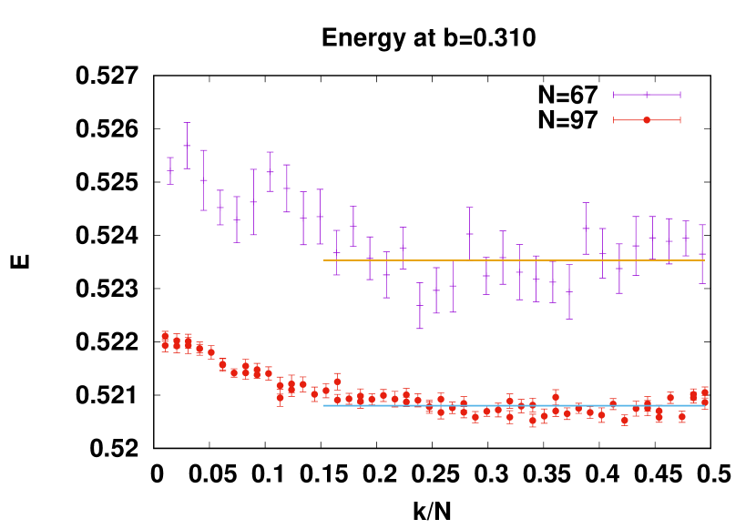
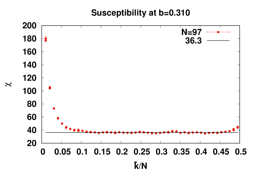
The pattern repeats itself for other values of $N$. As $N$ increases the left peak becomes narrower but at the value $k=\bar{k}=1$ actually increases. This is consistent with the observation of Ref. Profumo:2002cm . For completeness we give the values obtained for all our values of $N$. The susceptibility at $k=\bar{k}=1$ takes the values 50, 91, 102, 127, 137, 172, 180 and 226 for the sequence of values $N$=23, 43, 53, 61, 67, 89, 97 and 137. The growth seems to go as $N$ at smaller values, which then reduces to $\sim N^{1/2}$.

What is the origin of the peak? For the purpose of answering the question, we analyzed the correlator at the maximum distance $N/2$: $\bar{G}_{R}(N/2)$. For a gapped theory it should go to zero when $N$ grows. A non-zero asymptotic value reflects a non-vanishing expectation value. With the standard definition a non-zero expectation value gives a susceptibility diverging with the volume (in our case $N^{2}$). It is possible to subtract this constant piece and define a new susceptibility. Indeed, if we take our result and subtract $CN^{2}\bar{G}_{R}(N/2)$ with $1<C<1.025$ we eliminate the peak for all values of $N$.

Our prescription is, however, much simpler and compliant with the one adopted for the 2+1 and 3+1 dimensional gauge theories GonzalezArroyo:2010ss -Perez:2013dra . As explained in the introduction one should take the continuum limit keeping both $k/N$ and $\bar{k}/N$ bigger than a certain threshold which is roughly equal to 0.1. Indeed, a better way to select the adequate values of $k$ is to constrain the quantity $Z_{\mathrm{min}}(N,k)$, defined by Eq. (1), to be larger than that same value. A good test that this criteria eliminates the problems associated with the non-zero expectation value is to plot $\bar{G}_{R}(N/2)$ as a function of $N$. Our data give a neat exponential fall-off of the form $0.278\exp{(-0.176N/2)}$ until the moment that this value is smaller than the statistical errors ($N\sim 97$). The fall-off is the characteristic one for a gapped theory with no expectation value.

In conclusion, we emphasize that, also for the two-dimensional principal chiral model, it is convenient to adopt the same criteria for flux selection as advocated in Ref. GonzalezArroyo:2010ss . As mentioned in the introduction, for the 2+1 dimensional case Chamizo:2016msz -newtwoplusone we observed that this choice avoids the presence of symmetry-breaking phase transitions at $N$ large. However, even if no transition is present it is still very important for practical purposes to reduce the size of the finite $N$ corrections. In the following sections we will adopt this criteria and we will explore the behaviour of the reduced model at large $N$ both on the lattice and in the continuum limit.

4 Validity of reduction at large $N$

In this section we make a precision study of the validity of the volume independence hypothesis for the case of the two-dimensional principal chiral model. A successful test was already done in Ref. Profumo:2002cm for 3 and 4 dimensions. The test for the 2-dimensional model failed for the reasons explained in the previous section. Having identified the source of the problem we will retake the original goal. Notice, that it is not only a question of proving the validity but also a way to estimate the errors associated to finite $N$. Our study is very similar to the one done by the present authors Gonzalez-Arroyo:2014dua for Wilson loops on the TEK model.

Sticking first to the value b=0.31 of the lattice coupling, we summarize our results in Fig. 2. The left plot focuses on the internal energy $E$ and the right one on the susceptibility $\chi$. The data points labelled as AVERAGES correspond to the results mentioned on the previous section averaged over all values of the flux $k$ satisfying the criteria $Z_{\mathrm{min}}(N,k)\geq 0.15$. We have also added other measurements performed at single flux values but satisfying the same criteria. The $N$-dependence of the results shows two regimes. One up to values of the order of $N=50$ which is rather flat, and one for larger values which is consistent with a $1/N^{2}$ linear dependence. Extrapolating the results to infinite $N$ we get $E_{\infty}=0.5190(2)$ and $\chi_{\infty}=34.4(2)$. These values are consistent with the values obtained by previous authors from extrapolation in the ordinary lattice model (0.519 and 34.1(2) respectively). We have also made our own high-precision simulation in a $64\times 64$ lattice at $N=64$ and periodic boundary conditions. Our results are $E=0.519004(13)$ and $\chi=34.67(4)$. Thus, within the precision of our results (a permille and a percent respectively) we have verified that the reduced model tends to the infinite volume lattice model at large $N$.

(a) Internal Energy.

(b) Susceptibility.

Figure 2: $N$ dependence of physical quantities at $b=0.31$. Points labeled AVERAGES are obtained for the TRPCM averaging over various values of $k$. The single flux correspond to other measurements at fixed value of $k$. The points labeled $L=2,3$ are obtained for an $L\times L$ lattice with twisted boundary conditions.

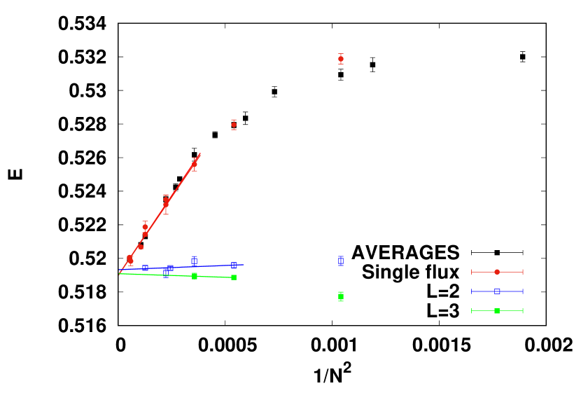
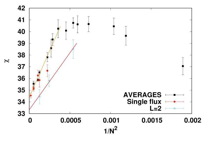
We have also studied the coupling value $b=0.32$. In that case we did not scan all values of $k$ but simply chose appropriate ones according to our criteria. In particular we studied several values of $N$ (43, 53, 67, 89, 97, 131, 137, 233). The results of the energy could be fitted (with good chi square) by the function $E=0.485758(15)+2.7(2)/N^{2}$. This matches with the rough estimate $0.485$ given in Ref. Profumo:2002cm . The situation for the susceptibility is not that good. A good fit to a linear function in $1/N^{2}$ is only possible for $N>67$. The extrapolated result at $N=\infty$ is 63.4(6) which is not too far from the estimate of 65 provided earlierProfumo:2002cm . The coefficient of $1/N^{2}$ being huge ($\sim 120000$). Although our results for the reduced model do not seem to be in conflict with those of the ordinary lattice model, a more precise comparison would require more statistics for the ordinary model simulation.

As mentioned in Ref. Profumo:2002cm the $N$-dependence is rather strong compared with that of the ordinary model. To a large extent this is because the $N$-dependence takes the role of the volume dependence which for the ordinary model is much stronger. For example, the value of the energy for the ordinary model with $N=43$ on a $6\times 6$ lattice with periodic boundary conditions is 0.4889, which is much further away from the infinite volume result than any of twisted results. In any case, it is clear that taking twisted boundary conditions pays off. For example, one can study a model reduced to a $2\times 2$ box with twisted boundary conditions (a matrix model of 4 matrices instead of 1). In that case the corresponding values of the energy and susceptibility also appear in the plot under the label $L=2$. The plot also contains (under the label $L=3$) the results obtained on a $3\times 3$ lattice with twisted boundary conditions. For the energy the $L=2$ data are independent on $N$ within errors. This is in part accidental, as there is a compensation of finite volume errors which tend to raise the value with the genuine finite $N$ corrections of the ordinary SU(N) model which tend to decrease it. In particular, we mention that the results at $N=64$ but using twisted boundary conditions with $k=19$ on a $2\times 2$ lattice gives $E=0.51946(5)$ and $\chi=35.8(5)$, and in a $3\times 3$ lattice $E=0.51918(10)$ and $\chi=35.94(35)$. At $b=0.32$ we also studied the twisted model on a $2\times 2$ lattice and N=67. The energy becomes $E=0.48569(5)$ and the susceptibility becomes $\chi=70.2(9)$.

Our comment about the ”partially reduced” model could be of practical importance for simulations. The larger number of degrees of freedom might pay off. This also neutralizes a similar criticism presented by Profumo and Vicari. For example, they studied a lower value of $b$ ($b=0.28$). In that case, they observed convergence of the reduced model results towards the ordinary model at large $N$. However, they observed that in the coefficient of the $1/N^{2}$ corrections was two orders of magnitude larger for the reduced model. For example, they obtained at $N=30$ a value of the susceptibility of $9.49(3)$ to be compared with the large $N$ result estimated to be 7.02(2). We have performed the measurement on a $2\times 2$ twisted box with flux $k=11$ and we obtained $7.09(5)$. The correction then is then not much bigger than the one of the ordinary model.

5 Continuum limit

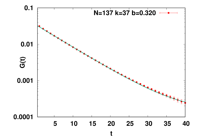
In this section we will study the reduced model in the continuum limit and compare it with the exact results that we have for this model. To be precise we will concentrate on the calculation of the mass gap $m$ extracted from the zero-momentum projection of the propagator $\bar{G}_{R}(t)$. For that purpose we simulated the reduced model for various values of $b$ ranging from $b=0.3$ up to $0.37$ and various values of $N$ (67,89, 97 and 137). We will concentrate here on the $N=137$ data for which we have a much higher statistics. In that case we generated 120000 configurations separated by 100 sweeps between each two. We did this for two different fluxes $k=37$ and $50$. For each configuration we computed the zero-momentum correlator $\bar{G}_{R}(t)$ with errors estimated by jacknife. As a sample of the quality of the data we show in Fig. 3(a) the correlator for $b=0.32$ and $k=37$. The data is then fitted to a 3 parameter formula as follows:

$$A+B\exp(-Mt).$$ (22)

In this way we obtain a lattice mass $M$ as a function of $b$. Using the fitting range $5\leq t\leq 25$ we obtain good fits with chi square per degree of freedom smaller than 1. The corresponding fit for $b=0.32$ is shown as a solid line in Fig. 3(a).

According to the scaling analysis explained earlier, we consider that our lattice mass $M$ equals $ma_{E}(b)$, where $a_{E}$ is given in Eq. (13). Substituting we obtain

$$M=\frac{m}{\Lambda_{E}}F(b_{E})$$ (23)

which according to scaling should hold asymptotically for large $b$. In Fig. 3(b) we plot the ratio $M/F(b_{E})$ obtained from our data in the weak coupling region ($b>0.306$; The $b_{E}$ scheme is singular below). The result is remarkably constant to within $3\%$ in the whole range. This is quite non-trivial as $F(b_{E})$ is three times larger in lower edge than in the upper edge of the displayed region. Furthermore, the constant is predicted to be

$$\frac{m}{\Lambda_{E}}=\frac{m}{\Lambda_{\overline{MS}}}\ \frac{\Lambda_{\overline{MS}}}{\Lambda_{L}}\ \frac{\Lambda_{L}}{\Lambda_{E}}=16\sqrt{\frac{\pi}{e}}\ \frac{\sin(\pi/N)}{\pi/N}\,\exp\{\pi\frac{N^{2}-1}{4N^{2}}\}=37.72.$$ (24)

This value is displayed as the orange line in the figure. The agreement is remarkable. Nonetheless, it must be mentioned that our result has systematic errors which are estimated to be of order $5\%$. This comes from changes in the fitting range and the choice of $k$. Smaller values of $N$ give similar results but the plateau is shorter.

(a) Correlator $\bar{G}_{R}(t)$.

(b) Determination of $m/\Lambda_{E}$. The horizontal line is the continuum prediction.

Figure 3: Analysis of the correlator and scaling.

A few comments on our result are necessary. The first concerns the constant term $A$ in the fitting formula. This term is needed to get high precision fits for $b>0.31$. This constant term actually grows as $b$ grows. Comparing similar fits for smaller values of $N$, one sees that the constant decreases with $N$. This is presumably also related with the non-zero value of $\mathrm{Tr}(U)$ observed at even larger values of $b$. Indeed, its phase takes a longer time to jump to different values, which demands impractically long simulations in order to see $\mathrm{Tr}(U)$ averaging out to zero. The phenomenon is not a phase transition because for finite $N$ there cannot be phase transitions and indeed at fixed $b$ the phenomenon is ameliorated when $N$ grows. It can be regarded as a phenomenon similar to a topology freezing. A genuine large $N$ phase transition of our model, replicating the one of the principal chiral model takes place at smaller values of $b$, and will be the subject of the next section.

A final comment is that adding a second exponential one can fit all the correlation functions in the full range (including zero). The lowest mass is compatible with the values obtained before, and the additional mass is around 4 times bigger than this. The coupling to the state is around 0.1 times the corresponding one of the lower mass state.

6 Analysis of the large $N$ phase transition

More than twenty years ago, Campostrini, Rossi and Vicari Campostrini:1994ih studied the large $N$ behavior of the $SU(N)$ lattice chiral model by Monte Carlo simulations with $N$ in the range $9\leq N\leq 30$. They found that the specific heat has a peak around $b=0.306$, whose height grows as $N$ increases, suggesting that there is a large $N$ second order phase transition. The reduced model allows us to reach much bigger values of $N$ so we can analyze the existence and nature of the phase transition in greater depth. The purpose of this section is to present the results of our study of the TRPCM around $b=0.306$ with $N$ in the range $67\leq N\leq 233$.

Figure 4: Time history of the internal energy $E$ of the ordinary lattice chiral model.

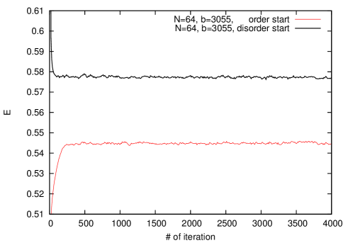
Apart from studying the TRPCM we also explored the ordinary lattice model on a $64\times 64$ lattice at $b=0.3055$ and $N=64$. In fig. 4 we show the time history of the internal energy $E$ starting from both ordered and disordered configurations. The pattern shows two different values for each starting configuration, suggesting that the phase transition is first order rather than second order. The amount of computer time required, due to the large number of degrees of freedom, limited the number of iterations of the model to 4000 in each case.

Figure 5: Time history of the internal energy $E$ of the TRPCM. Except $N=233$, the values of $E$ are shifted upward to make the figure readable.

Figure 6: Histogram of the internal energy $E$ of the TRPCM.

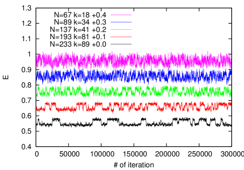
At $b=0.306$ we have run $1.2\times 10^{7}$ Monte Carlo iterations for the TRPCM with $N=67,89,137,193$ and 233. In Fig. 5, we show the time history of $E$ for the first 300000 iterations, plotting only the values every 100 iterations. The actual values have been displaced vertically to allow all values of $N$ to be put in the same plot. It is clear that at $N=67$, the fluctuations of the internal energy are much bigger than those of the ordinary lattice chiral model with $N=64$ shown in Fig. 4. This is expected since the Energy of the ordinary model is an average over the $64\times 64$ points of space.

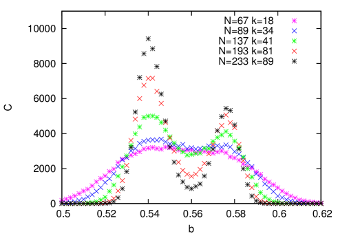
As we increase $N$ the dispersion of the internal energy of the TRPCM decreases and the existence of two different states becomes clear. This can be also seen by looking at the histogram of $E$ values displayed in fig. 6. The two peak structure becomes better defined as $N$ increases, while the peak positions do not seem to change much. This is all pointing towards the first order character of the transition.

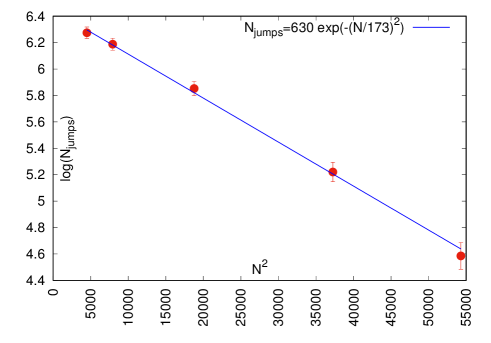
It is also clear from Fig. 5 that the number of flip-flops between both states is decreasing as $N$ increases. To quantify this phenomenon, we smoothen out the fluctuations by averaging the measurements in groups of 10. Then we count the number of jumps from one phase to the other $N_{jumps}$. The logarithm of the values are displayed versus $N^{2}$ in fig. 7, together with a linear fit to the data. This implies that the number of jumps decreases exponentially with the number of degrees of freedom of the system ($N^{2}$), or conversely that the tunneling times grow proportionally to the inverse of this number. This is precisely the expected behaviour for a large $N$ phase transition. Incidentally, the values are consistent with the presence of no jumps in the 4000 iterations of the ordinary model at $N=64$. To make a final check we performed $3\times 10^{6}$ iterations at $N=377$ with $k=233$ and found no flip-flops.

Figure 7: The logarithm of the number of flip-flop jumps $N_{jumps}$ between the two phases as a function of $N^{2}$ .

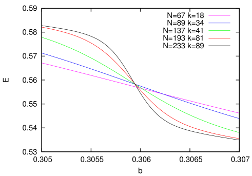
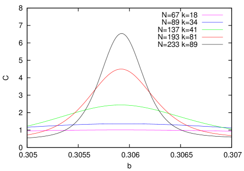
We also studied the $b$ dependence of $E$ and the specific heat $C=4b^{2}N^{2}(<E^{2}>-<E>^{2})$ close to the phase transition by the re-weighting method. Fig. 8 and 9 show the results of these analysis. If the transition is second order, the peak height of C should behave as $C_{max}(N)\sim N^{\alpha}$ with $\alpha$ the critical index characterizing a second order phase transition. However, $C_{max}(N)$ seems to be approaching a growth with the exponent $\alpha=2$ characteristic of a first order phase transition. Actually using the peak values for the two largest values of $N$ (233 and 193) the value of $\alpha$ is found to be $1.985$. At the same time the profile for $E$ approaches a step function.

Figure 8: $b$ dependence of the internal energy $E$ for $N=67,89,137,193$ and 233.

Figure 9: $b$ dependence of the specific heat $C$ for $N=67,89,137,193$ and 233.

If the large $N$ phase transition were of second order, the correlation length should diverge as we approach the phase transition. This is certainly not consistent with what we observe when coming from the ordered phase. From our data at $N=233$ our measured correlation lengths for $b=0.307,0.308,0.309$ and $0.310$ are (in lattice units) $3.82(2),4.12(4),4.45(10)$ and $4.61(20)$ respectively. Errors include systematics. We also determined the correlation length at $b=0.306$ from the ordered data at $N=377$ being $3.64(8)$.

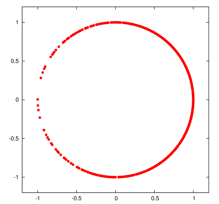
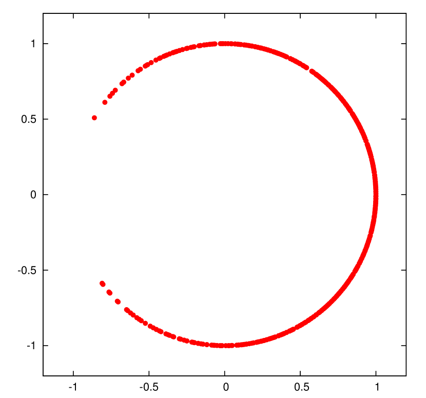
Given that the transition is first order one might wonder about the different behaviour of observables in the two phases, apart from the value of the energy $E$. For that purpose we calculated the eigenvalue distribution of $U\Gamma_{\mu}U^{\dagger}\Gamma_{\mu}^{\dagger}$ in both ordered and disordered states. To this end, we selected 30000th and 60000th $N=233$ configurations shown in Fig. 5. The eigenvalue distribution are shown in Fig. 10(a) for the disordered 30000th configuration and in Fig. 10(b) for the ordered 60000th configuration. It is clear that the eigenvalue distributions are quite different in the two phases.

(a) Disordered phase.

(b) Ordered phase.

Figure 10: Eigenvalue distribution of $U\Gamma_{\mu}U^{\dagger}\Gamma_{\mu}^{\dagger}$.

7 Conclusions and Outlook

In this paper we have re-examined the matrix model obtained by applying the twisted reduction procedure to the principal chiral model. Earlier, the two-dimensional model was found to give controversial results in its claim to be equivalent to the ordinary model at large $N$. Due to the new information acquired lately about similar issues of the reduced gauge theory model, we have been able to show that the difficulties can be avoided by choosing adequately the integer flux appearing in twisted boundary conditions. The criteria are very much the same as the ones found in gauge theories. Applying these guidelines we were able to show with great numerical precision that the results of the reduced and ordinary models agree within errors. Concerning the finite $N$ corrections its size also gets reduced by the choice of flux. An even stronger reduction is obtained by using only a partial reduction Narayanan:2003fc -GonzalezArroyo:2005dz to a twisted $2\times 2$ or $3\times 3$ box. It is beyond any doubt that using twisted boundary conditions in the study of this model pays off.

Our test of the reduced model has been extended to the continuum limit where it can be directly tested against exact results obtained for the principal chiral model. Our results also give conclusive evidence of scaling as dictated by the beta function of the model.

Finally, we have used the reduced model to investigate the interesting issue of the large $N$ phase transition of the principal chiral model. The larger values of $N$ that can be reached are an important benefit when studying this problem. Our conclusion is that the transition is actually of first order nature.

The simplicity of the TRPCM (a single unitary matrix model) makes it suitable for future studies including attempts of an exact solution. Several open problems, already mentioned in the introduction, could be analyzed.

References

- (1) E. Abdalla, M. C. B. Abdalla, A. Lima-Santos, Phys. Lett. B140 (1984) 71.
- (2) P. Wiegmann, Phys. Lett. B142 (1984) 173.
- (3) J. Balog, S. Naik, F. Niedermayer, P. Weisz, Phys. Rev. Lett. 69 (1992) 873.
- (4) M. Hasenbusch, S. Meyer, Phys. Rev. Lett. 68 (1992) 435.
- (5) P. Rossi, E. Vicari, Phys. Rev. D49 (1994) 1621 [hep-lat/9307014].
- (6) P. Rossi, E. Vicari, Phys. Rev. D49 (1994) 6072 Erratum: [Phys. Rev. D 50 (1994) 4718] Erratum: [Phys. Rev. D 55 (1997) 1698] [hep-lat/9401029].
- (7) F. Green, S. Samuel, Phys. Lett. B103 (1981) 110.
- (8) M. Campostrini, P. Rossi, E. Vicari, Phys. Rev. D52 (1995) 395 [hep-lat/9412102].
- (9) P. Orland, Phys. Rev. D 84 (2011) 105005 [arXiv:1108.0058 [hep-th]].
- (10) R. Narayanan, H. Neuberger, E. Vicari, JHEP 0804 (2008) 094 [arXiv:0803.3833 [hep-th]].
- (11) R. Narayanan, H. Neuberger, JHEP 0603 (2006) 064 [hep-th/0601210].
- (12) R. Narayanan, H. Neuberger, JHEP 0712 (2007) 066 [arXiv:0711.4551 [hep-th]].
- (13) A. Cherman, D. Dorigoni, G. V. Dunne and M. Ünsal, Phys. Rev. Lett. 112 (2014) 021601 [arXiv:1308.0127 [hep-th]].
- (14) T. Eguchi, H. Kawai, Phys. Rev. Lett. 48 (1982) 1063.
- (15) G. Bhanot, U. M. Heller, H. Neuberger, Phys. Lett. B113 (1982) 47.
- (16) A. Gonzalez-Arroyo, M. Okawa, Phys. Lett. B120 (1983) 174.
- (17) A. Gonzalez-Arroyo, M. Okawa, Phys. Rev. D27 (1983) 2397.
- (18) G. Parisi, Phys. Lett. B112 (1982) 463.
- (19) T. Eguchi and R. Nakayama, Phys. Lett. 122B (1983) 59.
- (20) A. Gonzalez-Arroyo, M. Okawa, Nucl. Phys. B247 (1984) 104.
- (21) S. R. Das and J. B. Kogut, Nucl. Phys. B 235 (1984) 521.
- (22) J. Ambjorn, Y. M. Makeenko, J. Nishimura and R. J. Szabo, JHEP 9911 (1999) 029 [hep-th/9911041].
- (23) A. Gonzalez-Arroyo and C. P. Korthals Altes, Phys. Lett. 131B (1983) 396.
- (24) S. Profumo, JHEP 0210 (2002) 035 [hep-th/0111285].
- (25) S. Profumo, E. Vicari, JHEP 0205 (2002) 014 [hep-th/0203155].
- (26) T. Ishikawa and M. Okawa, talk given at the Annual Meeting of the Physical Society of Japan, March 28-31, Sendai, Japan (2003).
- (27) W. Bietenholz, J. Nishimura, Y. Susaki and J. Volkholz, JHEP 0610 (2006) 042 [hep-th/0608072].
- (28) M. Teper, H. Vairinhos, Phys. Lett. B652 (2007) 359-369. [hep-th/0612097].
- (29) T. Azeyanagi, M. Hanada, T. Hirata, T. Ishikawa, JHEP 0801 (2008) 025 [arXiv:0711.1925 [hep-lat]].
- (30) A. Gonzalez-Arroyo, M. Okawa, JHEP 1007 (2010) 043 [arXiv:1005.1981 [hep-th]].
- (31) A. Gonzalez-Arroyo and M. Okawa, JHEP 1412 (2014) 106 [arXiv:1410.6405 [hep-lat]].
- (32) A. Gonzalez-Arroyo, M. Okawa, Phys.Lett. B718 (2013) 1524.
- (33) M. García Pérez, A. González-Arroyo and M. Okawa, JHEP 1309 (2013) 003 [arXiv:1307.5254 [hep-lat]].
- (34) M. Garcia Perez, A. Gonzalez-Arroyo and M. Okawa, Int. J. Mod. Phys. A 29 (2014) 1445001 [arXiv:1406.5655 [hep-th]].
- (35) F. Chamizo and A. Gonzalez-Arroyo, J. Phys. A 50 (2017) 265401 [arXiv:1610.07972 [hep-th]].
-
(36)
M. Garcia Perez, A. Gonzalez-Arroyo, M. Koren and M. Okawa,
” The spectrum of a 2+1 dimensional Yang-Mills theory on a twisted
spatial torus”
In preparation. - (37) A. M. Polyakov, Phys. Lett. B72 (1977) 224.
- (38) N. D. Mermin, H. Wagner, Phys. Rev. Lett. 17 (1966) 1133.
- (39) S. R. Coleman, Commun. Math. Phys. 31 (1973) 259.
- (40) P. Rossi, M. Campostrini and E. Vicari, Phys. Rept. 302 (1998) 143 [hep-lat/9609003].
- (41) A. McKane, M. Stone, Nucl. Phys. B163 (1980) 169.
- (42) J. Shigemitsu, J. B. Kogut, Nucl. Phys. B190 (1981) 365.
- (43) M. Campostrini, P. Rossi, E. Vicari, Phys. Rev. D52 (1995) 386 [hep-lat/9412101].
- (44) K. Fabricius and O. Haan, Phys. Lett. B 143 (1984) 459.
- (45) M. García Pérez, A. González-Arroyo, L Keegan, M. Okawa and A. Ramos, JHEP 1506 (2015) 193 [arXiv:1505.05784 [hep-lat]].
- (46) R. Narayanan and H. Neuberger, Phys. Rev. Lett. 91 (2003) 081601 [hep-lat/0303023].
- (47) A. Gonzalez-Arroyo, R. Narayanan and H. Neuberger, Phys. Lett. B 631 (2005) 133 [hep-lat/0509074].