Algorithm for Lens Calculations in the Geometrized Maxwell Theory

Abstract

Nowadays the geometric approach in optics is often used to find out media parameters based on propagation paths of the rays because in this case it is a direct problem. However inverse problem in the framework of geometrical optics is usually not given attention.

The aim of this work is to demonstrate the work of the proposed the algorithm in the framework of geometrical approach to optics for solving the problem of finding the propagation path of the electromagnetic radiation depending on environmental parameters. The methods of differential geometry are used for effective metrics construction for isotropic and anisotropic media. For effective metric space ray trajectories are obtained in the form of geodesic curves. The introduced algorithm is applied to well-known objects — Maxwell and Luneburg lenses. The similarity of results obtained by classical and geometric approach is demonstrated.

I Introduction

Geometrical approach to Maxwell’s equations has passed through several stages in its development. Initial interest was caused by the General theory of relativity. The works of L. I. Mandelstam, I. E. Tamm tamm:1924:jrpc::en ; tamm:1925:jrpc::en ; tamm:1925:mathann , W. Gordon gordon:1923 belong to this period. In the absence of practical applications the interest for this subject has gone. A new surge of interest arose during the Golden age of the theory of relativity (1960–1975). The works of J. Plebanski plebanski:1960:electromagnetic_waves , F. Felice felice:1971:as_optical_medium belong to this period. However, it should be note that in this period scientists failed to determine the application of developed theory.

A new outbreak of interest in the geometric approach emerged in the mid 2000 as a side effect of the interest in metamaterials smolyaninov:2011:metamaterial . We shell mention the studies of J. B. Pendry pendry:2006:controlling-em ; schurig:2006:ray-tracing and U. Leonhardt leonhardt:2006:mapping ; leonhardt:2009:light . These works gave rise to the whole direction — transformational optics foster:2015:spatial_transformations .

For the classical approach to optics the direct and inverse problems are usually formulated as follows:

• the direct problem: from the environment settings to obtain the path of electromagnetic waves propagation;

• the inverse problem: from given propagations paths of electromagnetic waves to obtain environments parameters.

For the geometric approach to optics these problems are swapped:

• the direct problem: for a given distribution paths of electromagnetic waves to obtain environment (medium) parameters;

• the inverse problem: from parameters of the environment to obtain the propagation path of electromagnetic waves.

Therefore, transformation optics works with direct problem of geometric optics (the inverse problem of classical optics).

Usually, in the framework of geometrical optics only a direct problem is solved, i.e. the task of finding the parameters of the environment from the propagation path of electromagnetic waves. This framework does not focuses on the inverse problem, i.e. finding the propagation path of electromagnetic waves according to the known parameters of the medium.

This work aims to consistently present the algorithm of lenses calculations with use of geometrical optics approach and demonstrate the convergence of our results with the results of the classical optics approach.

The structure of this paper is following. In section II the basic notation and conventions used in the article are given. In section III we describe the algorithm for inverse problem of geometrical optics. In paragraph IV we present examples of calculation of specific lenses. The results of numerical experiment are presented in graphical form.

II Notations and conventions

1. We will use the notation of abstract indices penrose-rindler:spinors::en . In this notation tensor as a complete object is denoted merely by an index (e.g., $x^{i}$). Its components are designated by underlined indices (e.g., $x^{\underline{\vphantom{j}{i}}\,}$).

2. We will adhere to the following agreements. Greek indices ($\alpha$, $\beta$) will refer to the four-dimensional space, in the component form it looks like: $\underline{\vphantom{j}{\alpha}}\,=\overline{0,3}$. Latin indices from the middle of the alphabet ($i$, $j$, $k$) will refer to the three-dimensional space, in the component form it looks like: $\underline{\vphantom{j}{i}}\,=\overline{1,3}$.

III The algorithm of solving the inverse problem of geometrical optics

Although geometrical optics deals with the direct problem of obtaining environmental parameters from rays propagation trajectories, it is possible to solve the inverse problem: calculation of lenses parameters.

Let us consider several options for solving the inverse problem geometrical optics, namely, the cases of isotropic and anisotropic media.

We will use the following algorithm for solving the inverse problem.

1. Inputs are the environmental parameters such as the permittivity $\varepsilon_{ij}$ and the permeability $\mu_{ij}$ and the refractive index $n_{ij}$. If we take into account specifics of the geometrization based on quadratic metric, we have to consider only the refractive index.

2. From physical considerations, we choose ansatz for the effective metric tensor $g_{\alpha\beta}$.

3. Based on this ansatz we obtain the general form of effective metric tensor $g_{\alpha\beta}$. This process is iterative. There is no guarantee that the chosen ansatz will give the opportunity to obtain metric tensor. In this case we have to choose another ansatz.

4. By substituting specific values of the parameters of the environment, we will receive a specific implementation of an effective metric tensor $g_{\alpha\beta}$.

Having an effective metric tensor, we can solve geometrical Maxwell equations and obtain the desired propagation path of electromagnetic waves kulyabov:2016:pcs ; kulyabov:2013:springer:cadabra . In this paper we will use the geometric optics approximation born-wolf:principles_optics::en ; bruns:1895 . For this case, the rays will be propagated along the geodesic curve ll:2::en ; mtw::en :

$$\derivative[2]{x^{\gamma}}{t}+\Gamma_{\alpha\beta}^{\gamma}\derivative{x^{\alpha}}{t}\derivative{x^{\beta}}{t}=0,$$ (1)

where $x^{\gamma}(t)$ are coordinates of geodesic curve. The Christoffel symbols are defined as follows:

$$\Gamma_{\alpha\beta}^{\gamma}=\frac{1}{2}g^{\gamma\delta}\quantity(\partialderivative{g_{\alpha\delta}}{x^{\beta}}+\partialderivative{g_{\beta\delta}}{x^{\alpha}}-\partialderivative{g_{\alpha\beta}}{x^{\delta}}).$$ (2)

For calculations we use the following expressions for geometrized material equations:

$$\begin{gathered}D^{i}=\varepsilon^{ij}E_{j}+{}^{(1)}\gamma^{i}_{j}B^{j},\\ H_{i}=(\mu^{-1})_{ij}B^{j}+{}^{(2)}\gamma^{j}_{i}E_{j},\\ \varepsilon^{\underline{\vphantom{j}{i}}\,\underline{\vphantom{j}{j}}\,}=-\sqrt{-g}\quantity(g^{00}g^{\underline{\vphantom{j}{i}}\,\underline{\vphantom{j}{j}}\,}\textendash g^{0\underline{\vphantom{j}{i}}\,}g^{0\underline{\vphantom{j}{j}}\,}),\\ (\mu^{-1})_{\underline{\vphantom{j}{i}}\,\underline{\vphantom{j}{j}}\,}=\sqrt{-g}\varepsilon_{\underline{\vphantom{j}{m}}\,\underline{\vphantom{j}{n}}\,\underline{\vphantom{j}{i}}\,}\varepsilon_{\underline{\vphantom{j}{k}}\,\underline{\vphantom{j}{l}}\,\underline{\vphantom{j}{j}}\,}g^{\underline{\vphantom{j}{n}}\,\underline{\vphantom{j}{k}}\,}g^{\underline{\vphantom{j}{m}}\,\underline{\vphantom{j}{l}}\,},\\ {}^{(1)}\gamma^{i}_{j}={}^{(2)}\gamma^{i}_{j}=\sqrt{-g}\varepsilon_{\underline{\vphantom{j}{k}}\,\underline{\vphantom{j}{l}}\,\underline{\vphantom{j}{j}}\,}g^{0\underline{\vphantom{j}{k}}\,}g^{\underline{\vphantom{j}{i}}\,\underline{\vphantom{j}{l}}\,}.\end{gathered}$$ (3)

Next, let us consider the isotropic and anisotropic cases.

III.1 Isotropic case

Consider the implementation of the inverse problem of geometrization for isotropic case. We will consider the case of diagonal metrics. All spatial diagonal components of the metric tensor are equal to each other. Thus, consider the following ansatz for the metric tensor:

$$\begin{gathered}g_{\underline{\vphantom{j}{\alpha}}\,\underline{\vphantom{j}{\beta}}\,}=\matrixquantity(a^{2}&0&0&0\\ 0&-b^{2}&0&0\\ 0&0&-b^{2}&0\\ 0&0&0&-b^{2}),\\ g^{\underline{\vphantom{j}{\alpha}}\,\underline{\vphantom{j}{\beta}}\,}=\matrixquantity(a^{-2}&0&0&0\\ 0&-b^{-2}&0&0\\ 0&0&-b^{-2}&0\\ 0&0&0&-b^{-2}),\\ \sqrt{-g}=ab^{3}.\end{gathered}$$ (4)

From relations (3) we can write down the expressions for the permittivity and the permeability:

$$\begin{gathered}\varepsilon^{\underline{\vphantom{j}{i}}\,\underline{\vphantom{j}{j}}\,}=ab^{3}a^{-2}\matrixquantity(b^{-2}&0&0\\ 0&b^{-2}&0\\ 0&0&b^{-2})=\frac{b}{a}\matrixquantity(1&0&0\\ 0&1&0\\ 0&0&1)=\frac{b}{a}\delta^{\underline{\vphantom{j}{i}}\,\underline{\vphantom{j}{j}}\,},\\ \quantity(\mu^{-1})_{\underline{\vphantom{j}{i}}\,\underline{\vphantom{j}{j}}\,}=ab^{3}\matrixquantity(b^{-4}&0&0\\ 0&b^{-4}&0\\ 0&0&b^{-4})=\frac{a}{b}\matrixquantity(1&0&0\\ 0&1&0\\ 0&0&1)=\frac{a}{b}\delta_{\underline{\vphantom{j}{i}}\,\underline{\vphantom{j}{j}}\,}.\end{gathered}$$ (5)

From equations (5) we can write the permittivity and the permeability in the following form:

$$\begin{gathered}\varepsilon^{\underline{\vphantom{j}{i}}\,\underline{\vphantom{j}{j}}\,}=\varepsilon\delta^{\underline{\vphantom{j}{i}}\,\underline{\vphantom{j}{j}}\,},\quad\varepsilon=\frac{b}{a},\\ \quantity(\mu^{-1})_{\underline{\vphantom{j}{i}}\,\underline{\vphantom{j}{j}}\,}=\frac{1}{\mu}\delta_{\underline{\vphantom{j}{i}}\,\underline{\vphantom{j}{j}}\,},\quad\mu=\frac{b}{a}.\end{gathered}$$ (6)

From (6) it is clear that remains one free parameter. Let the free parameter be $b$. Then let:

$$a=\frac{b}{\varepsilon}.$$ (7)

Then, based on the ansatz (4) we may write the metric tensor:

$$g_{\underline{\vphantom{j}{\alpha}}\,\underline{\vphantom{j}{\beta}}\,}=\matrixquantity(\frac{b^{2}}{\varepsilon^{2}}&0&0&0\\ 0&-b^{2}&0&0\\ 0&0&-b^{2}&0\\ 0&0&0&-b^{2}).$$ (8)

We will focus on Tamm tamm:1924:jrpc::en ; tamm:1925:jrpc::en ; tamm:1925:mathann approach. Let:

$$b^{2}=\sqrt{\mu}.$$ (9)

Then the metric tensor (8) we may rewrite:

$$g_{\underline{\vphantom{j}{\alpha}}\,\underline{\vphantom{j}{\beta}}\,}=\matrixquantity(\frac{\sqrt{\mu}}{\varepsilon^{2}}&0&0&0\\ 0&-\sqrt{\mu}&0&0\\ 0&0&-\sqrt{\mu}&0\\ 0&0&0&-\sqrt{\mu}).$$ (10)

Or, considering the ratio:

$$\varepsilon^{ij}\quantity(\mu^{-1})_{jk}=\delta^{i}_{k},$$ (11)

it is possible to rewrite (10) as

$$g_{\underline{\vphantom{j}{\alpha}}\,\underline{\vphantom{j}{\beta}}\,}=\matrixquantity(\frac{1}{\varepsilon\sqrt{\mu}}&0&0&0\\ 0&-\sqrt{\mu}&0&0\\ 0&0&-\sqrt{\mu}&0\\ 0&0&0&-\sqrt{\mu}).$$ (12)

This ratio coincides with the solution proposed by Tamm tamm:1925:mathann . The expression (10) or (12) sets the effective geometry of the environment.

III.2 Anisotropic case

Consider the simplest version of anisotropic medium. For this let us consider the following ansatz for the metric tensor:

$$\begin{gathered}g_{\underline{\vphantom{j}{\alpha}}\,\underline{\vphantom{j}{\beta}}\,}=\matrixquantity((a_{0})^{2}&0&0&0\\ 0&-(a_{1})^{2}&0&0\\ 0&0&-(a_{2})^{2}&0\\ 0&0&0&-(a_{3})^{2}),\\ g^{\underline{\vphantom{j}{\alpha}}\,\underline{\vphantom{j}{\beta}}\,}=\matrixquantity((a_{0})^{-2}&0&0&0\\ 0&-(a_{1})^{-2}&0&0\\ 0&0&-(a_{2})^{-2}&0\\ 0&0&0&-(a_{3})^{-2}),\\ \sqrt{-g}=a_{0}a_{1}a_{2}a_{3}.\end{gathered}$$ (13)

From relations (3) we may write down the expressions for the permittivity and the permeability:

$$\varepsilon^{\underline{\vphantom{j}{i}}\,\underline{\vphantom{j}{j}}\,}=a_{0}a_{1}a_{2}a_{3}(a_{0})^{-2}\matrixquantity((a_{1})^{-2}&0&0\\ 0&(a_{2})^{-2}&0\\ 0&0&(a_{3})^{-2})=\matrixquantity(\varepsilon_{1}&0&0\\ 0&\varepsilon_{1}&0\\ 0&0&\varepsilon_{1}),$$ (14)

$$\begin{multlined}\quantity(\mu^{-1})_{\underline{\vphantom{j}{i}}\,\underline{\vphantom{j}{j}}\,}={}\\ {}=a_{0}a_{1}a_{2}a_{3}\matrixquantity((a_{2})^{-2}(a_{3})^{-2}&0&0\\ 0&(a_{3})^{-2}(a_{1})^{-2}&0\\ 0&0&(a_{1})^{-2}(a_{2})^{-2})={}\\ {}=\matrixquantity(\frac{1}{\mu_{1}}&0&0\\ 0&\frac{1}{\mu_{2}}&0\\ 0&0&\frac{1}{\mu_{3}}).\end{multlined}\quantity(\mu^{-1})_{\underline{\vphantom{j}{i}}\,\underline{\vphantom{j}{j}}\,}={}\\ {}=a_{0}a_{1}a_{2}a_{3}\matrixquantity((a_{2})^{-2}(a_{3})^{-2}&0&0\\ 0&(a_{3})^{-2}(a_{1})^{-2}&0\\ 0&0&(a_{1})^{-2}(a_{2})^{-2})={}\\ {}=\matrixquantity(\frac{1}{\mu_{1}}&0&0\\ 0&\frac{1}{\mu_{2}}&0\\ 0&0&\frac{1}{\mu_{3}}).$$ (18)

From (14) and (18) the permittivity and the permeability are obtained as follows:

$$\begin{gathered}\varepsilon_{1}=\frac{\sqrt{-g}}{(a_{0})^{2}(a_{1})^{2}},\quad\varepsilon_{2}=\frac{\sqrt{-g}}{(a_{0})^{2}(a_{2})^{2}},\quad\varepsilon_{3}=\frac{\sqrt{-g}}{(a_{0})^{2}(a_{3})^{2}},\\ \mu_{1}=\frac{(a_{2})^{2}(a_{3})^{2}}{\sqrt{-g}},\quad\mu_{2}=\frac{(a_{3})^{2}(a_{1})^{2}}{\sqrt{-g}},\quad\mu_{3}=\frac{(a_{1})^{2}(a_{2})^{2}}{\sqrt{-g}}.\end{gathered}$$ (19)

From (19) we may write the following relations:

$$\begin{gathered}\mu_{2}\mu_{3}=\frac{(a_{3})^{2}(a_{1})^{2}}{\sqrt{-g}}\frac{(a_{1})^{2}(a_{2})^{2}}{\sqrt{-g}}=\frac{(a_{1})^{4}}{\sqrt{-g}}\frac{(a_{2})^{2}(a_{3})^{2}}{\sqrt{-g}}=\frac{(a_{1})^{4}}{\sqrt{-g}}\mu_{1},\\ \mu_{3}\mu_{1}=\frac{(a_{1})^{2}(a_{2})^{2}}{\sqrt{-g}}\frac{(a_{2})^{2}(a_{3})^{2}}{\sqrt{-g}}=\frac{(a_{2})^{4}}{\sqrt{-g}}\frac{(a_{3})^{2}(a_{1})^{2}}{\sqrt{-g}}=\frac{(a_{2})^{4}}{\sqrt{-g}}\mu_{2},\\ \mu_{1}\mu_{2}=\frac{(a_{2})^{2}(a_{3})^{2}}{\sqrt{-g}}\frac{(a_{3})^{2}(a_{1})^{2}}{\sqrt{-g}}=\frac{(a_{3})^{4}}{\sqrt{-g}}\frac{(a_{1})^{2}(a_{2})^{2}}{\sqrt{-g}}=\frac{(a_{3})^{4}}{\sqrt{-g}}\mu_{3}.\end{gathered}$$ (20)

Let us write out the coefficients:

$$\begin{gathered}a_{1}=\sqrt{\frac{\mu_{2}\mu_{3}}{\mu_{1}}},\\ a_{2}=\sqrt{\frac{\mu_{3}\mu_{1}}{\mu_{2}}},\\ a_{3}=\sqrt{\frac{\mu_{1}\mu_{2}}{\mu_{3}}}.\end{gathered}$$ (21)

Thus, (13) is changed to:

$$g_{\underline{\vphantom{j}{\alpha}}\,\underline{\vphantom{j}{\beta}}\,}=\matrixquantity(\frac{1}{\sqrt{\varepsilon_{1}\varepsilon_{2}\mu_{3}}}&0&0&0\\ 0&-\sqrt{\frac{\mu_{2}\mu_{3}}{\mu_{1}}}&0&0\\ 0&0&-\sqrt{\frac{\mu_{3}\mu_{1}}{\mu_{2}}}&0\\ 0&0&0&-\sqrt{\frac{\mu_{1}\mu_{2}}{\mu_{3}}}).$$ (22)

It is easy to see that in the isotropic case, the ratio (22) proceeds in the ratio of (12). The expression (22) sets the effective geometry of the environment.

IV Examples of lenses calculation in geometrical optics

For examples of calculations we use a widely known Maxwell (fish-eye) maxwell:1854:fish-eye , and Luneburg luneburg:1964 lenses. Also, these lenses are important because for them one may obtain analytical solutions. In addition, convergence of solutions in the classical and geometrical approaches could be used for verification.

IV.1 Maxwell lens

Maxwell lens maxwell:1854:fish-eye is constructed so that, in special case, when the rays emit from a point source located one side of the lens, they are focused at one point on the opposite side of the lens.

The refractive index $n$ changes from $2n_{0}$ in the centre up to $n_{0}$ at the surface:

$$n(r)=\begin{dcases}\frac{2n_{0}}{1+\quantity(\frac{r}{R})^{2}},&r\leqslant R,\\ n_{0},&r>R.\end{dcases}$$ (23)

Here $R$ is the radius of the sphere or cylinder. Also usually one consider $n_{0}=1$. Since in the method of the geometrization based on quadratic metric the permittivity and the permeability are equal, so we can write:

$$\begin{gathered}\varepsilon^{\underline{\vphantom{j}{i}}\,\underline{\vphantom{j}{j}}\,}=\mu^{\underline{\vphantom{j}{i}}\,\underline{\vphantom{j}{j}}\,},\\ \varepsilon^{\underline{\vphantom{j}{i}}\,\underline{\vphantom{j}{j}}\,}=\varepsilon\delta^{\underline{\vphantom{j}{i}}\,\underline{\vphantom{j}{j}}\,},\quad\mu^{\underline{\vphantom{j}{i}}\,\underline{\vphantom{j}{j}}\,}=\mu\delta^{\underline{\vphantom{j}{i}}\,\underline{\vphantom{j}{j}}\,},\\ n=\sqrt{\varepsilon\mu}=\varepsilon=\mu,\\ \varepsilon=\mu=\frac{2}{1+\quantity(\frac{r}{R})^{2}},\quad r\leqslant R,n_{0}:=1.\end{gathered}$$ (24)

Then, from (12), we get the following metric:

$$g_{\underline{\vphantom{j}{\alpha}}\,\underline{\vphantom{j}{\beta}}\,}=\matrixquantity(\quantity(\frac{2}{1+\quantity(\frac{r}{R})^{2}})^{-3/2}&0&0&0\\ 0&-\quantity(\frac{2}{1+\quantity(\frac{r}{R})^{2}})^{1/2}&0&0\\ 0&0&-\quantity(\frac{2}{1+\quantity(\frac{r}{R})^{2}})^{1/2}&0\\ 0&0&0&-\quantity(\frac{2}{1+\quantity(\frac{r}{R})^{2}})^{1/2}).$$ (25)

Then we can depict the trajectories of rays as geodesic curves in this space (see Fig. 1). This figure shows that the behavior of the trajectories of the rays coincides with the theoretically predicted results from classical optics maxwell:1854:fish-eye , that is, the rays, emerging from source on the surface of the lens, are focused at a point located on the the opposite surface of the lens.

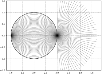
Figure 1: Ray trajectories as geodesic curves for Maxwell lens

IV.2 Luneburg Lens

Luneburg lens luneburg:1964 ; morgan:1958:luneberg_lens is the gradient lens. The refractive index changes depending on the distance from the center (spherical lens) or from the axis (cylindrical lens). With the passage of the lens the parallel rays are focused at one point on the surface of the lens. The rays emitted by a point source on the surface lenses form a parallel beam.

The refractive index $n$ changes from $\sqrt{2}n_{0}$ in the centre up to $n_{0}$ at the surface:

$$n(r)=\begin{dcases}n_{0}\sqrt{2-\quantity(\frac{r}{R})^{2}},&r\leqslant R,\\ n_{0},&r>R.\end{dcases}$$ (26)

Here $R$ is the radius of the sphere or cylinder. Also, usually one consider $n_{0}=1$.

Since in the method of the geometrization based on quadratic metric the permittivity and the permeability are equal, we can write:

$$\begin{gathered}\varepsilon^{\underline{\vphantom{j}{i}}\,\underline{\vphantom{j}{j}}\,}=\mu^{\underline{\vphantom{j}{i}}\,\underline{\vphantom{j}{j}}\,},\\ \varepsilon^{\underline{\vphantom{j}{i}}\,\underline{\vphantom{j}{j}}\,}=\varepsilon\delta^{\underline{\vphantom{j}{i}}\,\underline{\vphantom{j}{j}}\,},\quad\mu^{\underline{\vphantom{j}{i}}\,\underline{\vphantom{j}{j}}\,}=\mu\delta^{\underline{\vphantom{j}{i}}\,\underline{\vphantom{j}{j}}\,},\\ n=\sqrt{\varepsilon\mu}=\varepsilon=\mu,\\ \varepsilon=\mu=\sqrt{2-\quantity(\frac{r}{R})^{2}},\quad r\leqslant R,n_{0}:=1.\end{gathered}$$ (27)

Then, from (12), we get the following metric:

$$g_{\underline{\vphantom{j}{\alpha}}\,\underline{\vphantom{j}{\beta}}\,}=\matrixquantity(\quantity(2-\frac{r}{R})^{-3/4}&0&0&0\\ 0&-\quantity(2-\frac{r}{R})^{1/4}&0&0\\ 0&0&-\quantity(2-\frac{r}{R})^{1/4}&0\\ 0&0&0&-\quantity(2-\frac{r}{R})^{1/4}).$$ (28)

Then we can depict the trajectories of rays as geodesic curves in this space (see Fig. 2). This figure shows that the behavior of the trajectories of the rays coincides with the the theoretically prediction of classical optics morgan:1958:luneberg_lens . The rays, which emerge from a point source on the surface of the lens, form a parallel beam.

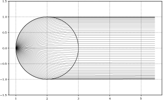
Figure 2: Ray trajectories as geodesic curves for Luneburg lens

V Conclusion

The authors proposed the algorithm for the calculation of the lenses in the framework of the geometrical approach to optics. The ansatzes for cases of isotropic and anisotropic media are proposed. For example, the widely known Luneburg and Maxwell lenses demonstrate a coincidence of the classical and geometric approaches. For simplicity the calculations were performed only for geometrical optics.

Unfortunately, it is not clear if the proposed approach for lens calculation on the basis of geometrical optics has any advantages over classical one. This question will be the subject of further research.

- (1) I. E. Tamm, Electrodynamics of an Anisotropic Medium in a Special Theory of Relativity, Russian Journal of Physical and Chemical Society. Part physical 56 (2-3) (1924) 248–262.
- (2) I. E. Tamm, Crystal Optics Theory of Relativity in Connection with Geometry Biquadratic Forms, Russian Journal of Physical and Chemical Society. Part physical 57 (3-4) (1925) 209–240.
- (3) I. E. Tamm, L. I. Mandelstam, Elektrodynamik der anisotropen Medien in der speziellen Relativitatstheorie, Mathematische Annalen 95 (1) (1925) 154–160.
- (4) W. Gordon, Zur Lichtfortpflanzung nach der Relativitätstheorie, Annalen der Physik 72 (1923) 421–456. doi:10.1002/andp.19233772202.
- (5) J. Plebanski, Electromagnetic Waves in Gravitational Fields, Physical Review 118 (5) (1960) 1396–1408. doi:10.1103/PhysRev.118.1396.
- (6) F. Felice, On the Gravitational Field Acting as an Optical Medium, General Relativity and Gravitation 2 (4) (1971) 347–357. doi:10.1007/BF00758153.
- (7) I. I. Smolyaninov, Metamaterial ‘Multiverse’, Journal of Optics 13 (2) (2011) 024004. arXiv:1005.1002, doi:10.1088/2040-8978/13/2/024004.
- (8) J. B. Pendry, D. Schurig, D. R. Smith, Controlling Electromagnetic Fields, Science 312 (5781) (2006) 1780–1782. doi:10.1126/science.1125907.
- (9) D. Schurig, J. B. Pendry, D. R. Smith, Calculation of Material Properties and Ray Tracing in Transformation Media, Optics express 14 (21) (2006) 9794–9804. arXiv:0607205, doi:10.1364/OE.14.009794.
- (10) U. Leonhardt, Optical Conformal Mapping, Science 312 (June) (2006) 1777–1780. arXiv:0602092, doi:10.1126/science.1218633.
- (11) U. Leonhardt, T. G. Philbin, Transformation Optics and the Geometry of Light, in: Progress in Optics, Vol. 53, 2009, pp. 69–152. arXiv:0805.4778v2, doi:10.1016/S0079-6638(08)00202-3.
- (12) R. Foster, P. Grant, Y. Hao, A. Hibbins, T. Philbin, R. Sambles, Spatial Transformations: from Tundamentals to Applications, Philosophical Transactions of the Royal Society A: Mathematical, Physical and Engineering Sciences 373 (2049) (2015) 20140365. doi:10.1098/rsta.2014.0365.
- (13) R. Penrose, W. Rindler, Spinors and Space-Time: Volume 1, Two-Spinor Calculus and Relativistic Fields, Vol. 1, Cambridge University Press, 1987. doi:10.1017/CBO9780511564048.
- (14) D. S. Kulyabov, Using two Types of Computer Algebra Systems to Solve Maxwell Optics Problems, Programming and Computer Software 42 (2) (2016) 77–83. arXiv:1605.00832, doi:10.1134/S0361768816020043.
- (15) A. V. Korol’kova, D. S. Kulyabov, L. A. Sevast’yanov, Tensor Computations in Computer Algebra Systems, Programming and Computer Software 39 (3) (2013) 135–142. arXiv:1402.6635, doi:10.1134/S0361768813030031.
- (16) M. Born, E. Wolf, Principles of Optics: Electromagnetic Theory of Propagation, Interference, and Diffraction of Light, 7th Edition, Cambridge University Press, Cambridge, 1999.
- (17) H. Bruns, Das Eikonal, Vol. 35, S. Hirzel, Leipzig, 1895.
- (18) L. D. Landau, E. M. Lifshitz, The Classical Theory of Fields, 4th Edition, Course of Theoretical Physics. Vol. 2, Butterworth-Heinemann, 1975.
- (19) C. W. Misner, K. S. Thorne, J. A. Wheeler, Gravitation, W. H. Freeman, San Francisco, 1973.
- (20) J. C. Maxwell, Solutions of Problems (prob. 3, vol. VIII, p. 188), The Cambridge and Dublin mathematical journal 9 (1854) 9–11.
- (21) R. K. Luneburg, Mathematical Theory of Optics, University of California Press, Berkeley & Los Angeles, 1964.
- (22) S. P. Morgan, General Solution of the Luneberg Lens Problem, Journal of Applied Physics 29 (9) (1958) 1358. doi:10.1063/1.1723441.