Linear Instability of Elliptic Rhombus Solutions to the Planar Four-body Problem

Abstract

In this paper, we study the linear stability of the elliptic rhombus solutions, which are the Keplerian homographic solution with the rhombus central configurations in the classical planar four-body problems. Using $\omega$-Maslov index theory and trace formula, we prove the linear instability of elliptic rhombus solutions if the shape parameter $u$ and the eccentricity of the elliptic orbit $e$ satisfy $(u,e)\in(1/\sqrt{3},u_{2})\times[0,\hat{f}(\frac{27}{4})^{-1/2})\cup(u_{2},1/u_{2})\times[0,1)\cup(1/u_{2},\sqrt{3})\times[0,\hat{f}(\frac{27}{4})^{-1/2})$ where $u_{2}\approx 0.6633$ and $\hat{f}(\frac{27}{4})^{-1/2}\approx 0.4454$. Motivated on numerical results of the linear stability to the elliptic Lagrangian solutions in [R. Martínez, A. Samà, and C. Simó, J. Diff. Equa., 226(2006): 619–651.], we further analytically prove the linear instability of elliptic rhombus solutions for $(u,e)\in(1/\sqrt{3},\sqrt{3})\times[0,1)$.

2010 MS classification: 58E05, 37J45, 34C25

Key words: linear stability, Morse index, $\omega$-Maslov index, hyperbolic region, elliptic rhombus solution, planar four-body problem.

Running title: Linear Instability of Elliptic Rhombus Solution.

1 Introduction

In the classical planar $N$-body problems of celestial mechanics, the position vectors of the $N$-particles are denoted by $q_{1},\dots,{q_{N}}\in{\bf R}^{2}$, and the masses are represented by $m_{1},\dots,{m_{N}}>0$. By Newton’s second law and the law of universal gravitation, the system of equations is

$$m_{i}\ddot{q_{i}}=\frac{\partial U}{\partial q_{i}},\quad i=1,{\dots,N},$$ (1.1)

where $U(q)=U(q_{1},{\dots,q_{N}})=\sum_{1\leq i<j\leq{N}}\frac{m_{i}m_{j}}{|q_{i}-q_{j}|}$ is the potential function and $|\cdot|$ is the standard norm of vector in ${\bf R}^{2}$. Suppose the configuration space is

$$\hat{\chi}:=\left\{q=(q_{1},{\dots,q_{N}})\in({\bf R}^{2})^{{N}}\left|\sum_{i=1}^{{N}}m_{i}q_{i}=0,q_{i}\neq q_{j},\forall i\neq j\right.\right\}.$$

For the period $T$, the corresponding action functional is

$$\mathbf{A}(q)=\int_{0}^{T}\left[\sum_{i=1}^{{N}}\frac{m_{i}|\dot{q}_{i}(t)|^{2}}{2}+U(q(t))\right]{\mathrm{d}}t,$$ (1.2)

which is defined on the loop space $W^{1,2}({\bf R}/T{\bf Z},\hat{\chi})$. The periodic solutions of (1.1) correspond to critical points of the action functional (1.2).

It is well-known that (1.1) can be reformulated as a Hamiltonian system. Let $p_{1},{\dots,p_{N}}\in{\bf R}^{2}$ be the momentum vectors of the particles respectively. The Hamiltonian system is given by

$$\dot{p}_{i}=-\frac{\partial H}{\partial q_{i}},\;\dot{q}_{i}=\frac{\partial H}{\partial p_{i}},\quad\mbox{for}\;i=1,{\dots,N},$$ (1.3)

with the Hamiltonian function

$$H(p,q)=\sum_{i=1}^{{N}}\frac{|p_{i}|^{2}}{2m_{i}}-U(q_{1},{\dots,q_{N}}).$$ (1.4)

One special class of periodic solutions to the planar $N$-body problem is the elliptic relative equilibrium (ERE for short) [18]. It is generated by a central configuration and the Keplerian motion. A central configuration is formed by $N$ position vectors $\left(q_{1},\ldots,q_{N}\right)=\left(a_{1},\ldots,a_{N}\right)$ which satisfy

$$-\lambda m_{i}q_{i}=\frac{\partial U}{\partial q_{i}},\forall\;1\leq i\leq N,$$ (1.5)

where $\lambda=U(a)/{I(a)}>0$ and $I(a)={\sum_{i=1}^{N}}m_{i}|a_{i}|^{2}$ is the moment of inertia. A planar central configuration of the $N$-body problem gives rise to a solution of (1.1) where each particle moves on a specific Keplerian orbit while the totality of the particles move according to a homothety motion. Namely, the motions of particles are homographic and the configuration is the same up to rotation and dilation (cf. Figure 1.1). If the Keplerian orbit is elliptic, then the solution is an equilibrium in pulsating coordinates. Readers may refer to [19] for detailed properties of the central configuration.

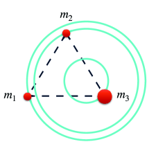
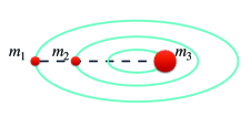
(a) The circular Lagrangian solution	(b) The elliptic Euler solution
(c) The elliptic rhombus solution	(d) The elliptic rhombus solution

Figure 1.1: We show three examples of the elliptic relative equilibria: the circular Lagrangian solution in (a), the elliptic Euler solution in (b), and the elliptic rhombus solution in (c) and (d). The blue lines represent the orbits of particles; and the dotted lines represent the central configurations: the equilateral triangle, the collinear configuration and the rhombus respectively. From (c) to (d), each particle moves counterclockwise in elliptic orbits and the totality of the particles move according to a homothety motion.

In this paper, we consider the linear stability of elliptic rhombus solutions to the planar four-body problem where the four particles form a rhombus central configuration. For four particles forming a convex quadrilateral central configuration, it is symmetric with respect to the diagonal if and only if two particles on the opposite sides of the diagonal possess equal masses [1]. Without loss of generality, suppose the masses of the four particles satisfy $m_{1}=m_{3}=m$, and $m_{2}=m_{4}=1$; and the positions satisfy $a=(a_{1}(u),a_{2}(u),a_{3}(u),a_{4}(u))^{T}$ (cf. (c) of Figure 1.1) where

$$a_{1}=\frac{1}{{\alpha}}(0,u),\;a_{2}=\frac{1}{{\alpha}}(1,0),\;a_{3}=\frac{1}{{\alpha}}(0,-u),\;a_{4}=\frac{1}{{\alpha}}(-1,0),$$ (1.6)

and ${\alpha}=\sqrt{2mu^{2}+2}$ is the re-scaling parameter. In short, the particles on the diagonal of the rhombus possess the same mass. By ${\alpha}=\sqrt{2mu^{2}+2}$, the moment of inertia $I(a)$ satisfies $I(a)=1$ and then ${\lambda}=U(a)$ in (1.5). By (1.5) and (5.10) of [14], $m$ and $u$ must satisfy

$$m=\frac{8u^{3}-u^{3}(1+u^{2})^{3/2}}{8u^{3}-(1+u^{2})^{3/2}},$$ (1.7)

where $1/\sqrt{3}<u<\sqrt{3}$. It has been proven that, for the given mass $m_{1}=m_{3}=m$ and $m_{2}=m_{4}=1$, the rhombus central configuration is unique [21]. The elliptic rhombus solution is one of the most intuitive ERE to the four-body problem because it is symmetric with respect to the two diagonals. Moreover, it is also one simple model of the double-ringed galaxy where the two bigger mass particles form the inner ring and the two smaller mass particles form the outer ring. For more details about the non-collinear symmetric central configuration of the four-body problem, readers may refer to [15] and [1] and the references therein.

The linear stability of the ERE is revealed by the eigenvalues of the linearized Poincaré map. Let ${\bf U}$ denote the unit circle in the complex plane. The ERE is linearly stable if the linearized Poincaré map is semi-simple and all its eigenvalues are on ${\bf U}$; it is linearly unstable if at least one pair of eigenvalues are not on ${\bf U}$; i.e., at least one pair of eigenvalues are hyperbolic. Since the nineteenth century [23], this has always been one of the active research topics in celestial mechanics, as it indicates the dynamics near these period orbits. Moreover, these results can be applied to the solar system and space mission design. For example, the sun, Jupiter and the Trojan asteroids form a Lagrangian configuration. Moreover, Chang’e 2 used the instability of ellipitic Euler solutions, which is formed by sun-Chang’e 2-earth, to travel to 4179 Toutatis and then into deep space.

However, it is difficult to obtain the linear stability of ERE, because the linearized Hamiltonian systems are non-autonomous, especially when the eccentricity of the orbit is not zero. In the three-body problems, many results related to linear stability have been obtained over the past decades by means of bifurcation theory [22], numerical methods [17] and the index theory [6, 3, 5, 25]. To the best of our knowledge, the ${\omega}$-Maslov index theory is the only analytical method to obtain the full picture of the stability and instability to the ERE, such as the elliptic Lagrangian solution (cf. (a) of Figure 1.1) [6, 3, 5], and the elliptic Euler solution (cf. (b) of Figure 1.1) [25, 26].

The stability of ERE when it comes to four-body problems is quite open. In 2017, Mansur, Offin and Lewis in [16] proved the instability of the constrained elliptic rhombus solution in reduced space. These authors used the minimizing property of the action functional and assumed the nondegeneracy of the variational problem. They then proved that the linearized Poincaré map possesses at least one pair of hyperbolic eigenvalues. If the orbits are circular, Ouyang and Xie obtained instability of the rhombus solution in the reduced space in [20]; i.e., the linearized Poincaré map possesses one pair of hyperbolic eigenvalues. For circular rhombus solutions of a homogeneous potential with degree $a$, Leandro in [9] obtained the condition for stability and instability with respect to $a$. Regarding the linear stability of other ERE to the four-body problem, readers may refer to [24], [2], and [10].

In this paper, we reduce the linearized linear Hamiltonian system with fundamental solution $\gamma_{0}(t)$ to three independent linear Hamiltonian systems of ${\gamma}_{1}(t)$, ${\gamma}_{u,e}(t)$ and $\eta_{u,e}(t)$ where ${\gamma}_{1}(t)$ corresponds to the Keplerian motion (cf. (2.29) below). This has been fully studied in [6]. The other two Hamiltonian systems of ${\gamma}_{u,e}(t)$ and $\eta_{u,e}(t)$ are the essential part for the stability where $u\in(1/\sqrt{3},\sqrt{3})$ is the shape parameter in (1.6) and $e\in[0,1)$ is the eccentricity of the elliptic orbit (cf. (2.30) and (2.31) below). We analyze the ${\omega}$-Maslov indices of ${\gamma}_{u,e}(t)$ and $\eta_{u,e}(t)$ using the ${\omega}$-Morse indices of the corresponding operators ${\cal A}(u,e)$ and ${\cal B}(u,e)$ (cf. (2.32) and (2.33) below). When $(u,e)\in\{1/\sqrt{3},u_{1}\}\times[0,1)$ (cf. $u_{1}$ in (ii) of Lemma 4.3 below), ${\cal A}(u,e)$ can be related to the linear stability of the elliptic Lagrangian solutions. We accordingly use the trace formula (cf. Theorem 1.8 of [5]) of the elliptic Lagrangian solutions to obtain the positive definiteness of ${\cal A}(u,e)$ in this region. Furthermore, the numerical results of the elliptic Lagrangian solutions (cf. Section 7 of [17]) can be used to extend the positive definiteness of ${\cal A}(u,e)$ to any eccentricity, i.e., $(u,e)\in\{1/\sqrt{3},u_{1}\}\times[0,1)$. The following lemma therefore holds:

Lemma 1.1.

• The operator ${\cal A}(u,e)$ is positive definite with zero nullity for any ${\omega}$-boundary condition and $(u,e)\in\{1/\sqrt{3}\}\times[0,\hat{f}(\frac{27}{4})^{-1/2})\cup\{{u_{1}}\}\times[0,\hat{f}({\beta}_{1})^{-1/2})$ where $\omega\in{\bf U}$ and $\hat{f}(\frac{27}{4})^{-1/2}\approx 0.4454$ and $\hat{f}({\beta}_{1})^{-1/2}\approx 0.4435$.

• The operator ${\cal A}(u,e)$ is positive definite with zero nullity for any ${\omega}$-boundary condition where $\omega\in{\bf U}$ and $(u,e)\in\{1/\sqrt{3},{u_{1}}\}\times[0,1)$.

We study the monotonicity of the operator ${\cal A}(u,e)$ and ${\cal B}(u,e)$ with respect to $u$ and compute their ${\omega}$-Morse indices. Together with Lemma 1.1 and the relationship between the ${\omega}$-Morse index and the ${\omega}$-Maslov index (cf. Lemma 2.4 below), we obtain the linear instability of the elliptic rhombus solution below, without the assumption on nondegeneracy.

Theorem 1.2.

• By (i) of Lemma 1.1, when $(u,e)\in(1/\sqrt{3},u_{2})\times[0,\hat{f}(\frac{27}{4})^{-1/2})\cup(u_{2},1/u_{2})\times[0,1)\cup(1/u_{2},\sqrt{3})\times[0,\hat{f}(\frac{27}{4})^{-1/2})$ where ${u_{2}}\approx 0.6633$, the linearized Poincaré map $\gamma_{0}(2\pi)$ possesses at least two pairs of hyperbolic eigenvalues; i.e., at least two pairs of eigenvalues are not on ${\bf U}$.

• By (ii) of Lemma 1.1, for $(u,e)\in(1/\sqrt{3},\sqrt{3})\times[0,1)$, ${\gamma}_{0}(2\pi)$ possesses four pairs of hyperbolic eigenvalues; i.e, all eigenvalues of the essential parts are hyperbolic.

We state this theorem separately because (i) of Theorem 1.2 is obtained by entirely analytical methods, while (ii) of Theorem 1.2 is the analytical results motivated by the numerical computations on elliptic Lagrangian solutions in [17].

The remainder of this paper is organized as follows. In Section 2, we reduce the linearized Hamiltonian system to three subsystems. In Section 3, we study the linear stability along three segments of the rectangle $(u,e)\in[1/\sqrt{3},\sqrt{3}]\times[0,1)$. In Section 4, we study the ${\omega}$-Maslov indices in the rectangle $(u,e)\in[1/\sqrt{3},\sqrt{3}]\times[0,1)$ and prove Theorem 1.2. We briefly review the ${\omega}$-Morse index and ${\omega}$-Maslov index theory in Section A of the Appendix and review the trace formula to yield the expression of $\hat{f}({\beta})$ in Section B of the Appendix.

2 Reduction of the Linearized Hamiltonian System

In this section, we use the symplectic reduction introduced in [18] to decompose the linearized Hamiltonian system into three independent Hamiltonian systems of ${\gamma}_{1}(t)$, ${\gamma}_{u,e}(t)$ and $\eta_{u,e}(t)$. The Hamiltonian system of ${\gamma}_{1}(t)$ in (2.29) corresponds to the Keplerian motion. The other two Hamiltonian systems of ${\gamma}_{u,e}(t)$ in (2.30) and $\eta_{u,e}(t)$ in (2.31) are called the essential parts whose linear stability will be discussed Section 3 and Section 4. After the reduction, we connect the two essential parts with the operators ${\cal A}(u,e)$ and ${\cal B}(u,e)$ respectively.

The Hessian of the potential $D^{2}U(q):=(B_{ij})_{4\times 4}$ at the central configuration $a$ is given by

$$\left.B_{ij}\right|_{q=a} :=\left.\frac{\partial^{2}U}{\partial q_{i}\partial q_{j}}\right|_{q=a}=\frac{m_{i}m_{j}}{|a_{i}-a_{j}|^{3}}\left(I-\frac{3(a_{j}-a_{i})(a_{j}-a_{i})^{T}}{|a_{i}-a_{j}|^{2}}\right),$$ (2.1)

$$\left.B_{ii}\right|_{q=a} :=\left.\frac{\partial^{2}U}{\partial q_{i}^{2}}\right|_{q=a}=\sum_{j\neq i}^{n}\frac{m_{i}m_{j}}{|a_{i}-a_{j}|^{3}}\left(-I+\frac{3(a_{i}-a_{j})(a_{i}-a_{j})^{T}}{|a_{i}-a_{j}|^{2}}\right).$$ (2.2)

By the symmetry of the configuration in (1.6), $a_{1}-a_{2}=a_{4}-a_{3}$ and $a_{2}-a_{3}=a_{1}-a_{4}$ hold. Via direct computations, we have $B_{12}=B_{34}$, $B_{14}=B_{23}$, and $B_{ij}=B_{ji}$ with $i\neq j$. Plugging (1.6) into (2.1), we have that

$${B_{12}} =\frac{{\alpha}^{3}m}{(1+u^{2})^{5/2}}\begin{pmatrix}u^{2}-2&3u\\ 3u&1-2u^{2}\end{pmatrix},\quad{B_{13}}=\frac{{\alpha}^{3}m^{2}}{8u^{3}}\begin{pmatrix}1&0\\ 0&-2\end{pmatrix},$$ (2.3)

$${B_{14}} =\frac{{\alpha}^{3}m}{(1+u^{2})^{5/2}}\begin{pmatrix}u^{2}-2&-3u\\ -3u&1-2u^{2}\end{pmatrix},\quad{B_{24}}=\frac{{\alpha}^{3}}{8}\begin{pmatrix}-2&0\\ 0&1\end{pmatrix}.$$ (2.4)

By $B_{ii}=-\sum_{j\neq i}B_{ij}$ in (2.1) and (2.2), it follows that

$$B_{11}=B_{33}= \frac{2{\alpha}^{3}m}{(1+u^{2})^{5/2}}\begin{pmatrix}2-u^{2}&0\\ 0&2u^{2}-1\end{pmatrix}+\frac{{\alpha}^{3}m^{2}}{8u^{3}}\begin{pmatrix}-1&0\\ 0&2\end{pmatrix};$$ (2.5)

$$B_{22}=B_{44}= \frac{2{\alpha}^{3}m}{(1+u^{2})^{5/2}}\left(\begin{matrix}2-u^{2}&0\\ 0&2u^{2}-1\end{matrix}\right)+\frac{{\alpha}^{3}}{8}\left(\begin{matrix}2&0\\ 0&-1\end{matrix}\right).$$ (2.6)

Suppose that

$$P=(p_{1},p_{2},p_{3},p_{4})^{T},Q=(q_{1},q_{2},q_{3},q_{4})^{T}.$$ (2.7)

We introduce the symplectic coordinate change from $(P,Q)^{T}$ to $(Y,X)^{T}$ by $P=A^{-T}Y$ and $Q=AX$, where $Y=(G,Z,W_{3},W_{4})^{T}$, $X=(g,z,w_{3},w_{4})^{T}$ and the matrix $A$ is given by

$$A=\begin{pmatrix}I&A_{12}&A_{13}&A_{14}\\ I&A_{22}&A_{23}&A_{24}\\ I&A_{32}&A_{33}&A_{34}\\ I&A_{42}&A_{43}&A_{44}\end{pmatrix}=\begin{pmatrix}1&0&0&-\frac{u}{{\alpha}}&-\frac{1}{\sqrt{2m+2}}&0&-\frac{1}{\sqrt{m}{\alpha}}&0\\ 0&1&\frac{u}{{\alpha}}&0&0&-\frac{1}{\sqrt{2m+2}}&0&-\frac{1}{\sqrt{m}{\alpha}}\\ 1&0&\frac{1}{{\alpha}}&0&\sqrt{\frac{m}{2m+2}}&0&0&\frac{u\sqrt{m}}{{\alpha}}\\ 0&1&0&\frac{1}{{\alpha}}&0&\sqrt{\frac{m}{2m+2}}&-\frac{u\sqrt{m}}{{\alpha}}&0\\ 1&0&0&\frac{u}{{\alpha}}&-\frac{1}{\sqrt{2m+2}}&0&\frac{1}{\sqrt{m}{\alpha}}&0\\ 0&1&-\frac{u}{{\alpha}}&0&0&-\frac{1}{\sqrt{2m+2}}&0&\frac{1}{\sqrt{m}{\alpha}}\\ 1&0&-\frac{1}{{\alpha}}&0&\sqrt{\frac{m}{2m+2}}&0&0&-\frac{u\sqrt{m}}{{\alpha}}\\ 0&1&0&-\frac{1}{{\alpha}}&0&\sqrt{\frac{m}{2m+2}}&\frac{u\sqrt{m}}{{\alpha}}&0\end{pmatrix}.$$ (2.8)

Via direct computations, we have $\tilde{J}A=A\tilde{J}$ and $A^{T}MA=I$ where $\tilde{J}={\rm diag}\{J_{2},J_{2},J_{2},J_{2}\}$, $J_{2}$ is the standard $2\times 2$ symplectic matrix, and $M={\rm diag}\{m_{1}I_{2},m_{2}I_{2},m_{3}I_{2},m_{4}I_{2}\}$. Through substitution of the new variables $(Y,X)^{T}$, the kinetic energy and the potential function are rewritten as

$$K= \frac{1}{2}(|G|^{2}+|Z|^{2}+|W_{3}|^{2}+|W_{4}|^{2}),$$ (2.9)

$$U(z,w_{3},w_{4})= \sum_{1<i\neq j<4}\frac{m_{i}m_{j}}{|(A_{i2}-A_{j2})z+\sum_{k=3}^{4}(A_{ik}-A_{jk})w_{k}|}.$$ (2.10)

By symplectic transformation, $z=z(t)$ is the Kepler elliptic orbit given through the true anomaly ${\theta}={\theta}(t)$,

$$r({\theta}(t))=|z(t)|=\frac{p}{1+e\cos{\theta}(t)},$$ (2.11)

where $p={l}(1-e^{2})$ and ${l}>0$ is the latus rectum of the ellipse. We paraphase the proposition of [18] (pp.271-273) and Proposition 2.1 of [26] in the case of $n=4$ and omit the proof.

Proposition 2.1.

There exists a symplectic coordinate change $\xi=(Z,W_{3},W_{4},z,w_{3},w_{4})^{T}\mapsto\bar{\xi}=(\bar{Z},\bar{W}_{3},\bar{W}_{4},\bar{z},\bar{w}_{3},\bar{w}_{4})^{T}$ such that, using the true anomaly ${\theta}$ as the variable, the resulting Hamiltonian function of the four-body problem in (1.4) is given by

$$H({\theta},\bar{Z},\bar{W}_{3},\bar{W}_{4},\bar{z},\bar{w}_{3},\bar{w}_{4})= \frac{1}{2}\left(|\bar{Z}|^{2}+\sum_{k=3}^{4}|\bar{W}_{k}|^{2}\right)+(\bar{z}^{T}J_{2}\bar{Z}+\sum_{k=3}^{4}\bar{w}_{k}^{T}J_{2}\bar{W}_{k})$$

$$+\frac{p-r({\theta})}{2p}\left(|\bar{z}|^{2}+\sum_{k=3}^{4}|\bar{w}_{k}|^{2}\right)-\frac{r({\theta})}{{\sigma}}U(\bar{z},\bar{w}_{3},\bar{w}_{4}),$$ (2.12)

where $r({\theta})=\frac{p}{1+e\cos{\theta}}$, $\mu{:=}U(a)=\frac{4m{\alpha}}{\sqrt{1+u^{2}}}+\frac{{\alpha}m^{2}}{2u}+\frac{{\alpha}}{2}$, ${\sigma}=(\mu p)^{1/4}$ and $p$ is given in (2.11).

Note that the elliptic rhombus solution $(P(t),Q(t))^{T}$ of (1.3) is in time $t$. Namely, $P(t)=M\dot{Q}(t)$ and $Q(t)=(r(t)R({\theta}(t))a_{1},r(t)R({\theta}(t))a_{2},r(t)R({\theta}(t))a_{3},r(t)R({\theta}(t))a_{4})^{T}$. By Proposition 2.1, $(P(t),Q(t))^{T}$ is transformed to the new solution $\xi_{0}{:=}(Y({\theta}),X({\theta}))^{T}$ in the variable true anomaly ${\theta}$ with respect to (2.12). In particular, $(Y({\theta}),X({\theta}))^{T}=(\bar{Z}({\theta}),\bar{W}_{3}({\theta}),\bar{W}_{4}({\theta}),\bar{z}({\theta}),\bar{w}_{3}({\theta}),\bar{w}_{4}({\theta}))^{T}$ with $G=g=0$. Moreover,

$$\xi_{0}=(0,\sigma,0,0,0,0,\sigma,0,0,0,0,0)^{T}\in{\bf R}^{12}.$$ (2.13)

For the sake of simplicity, we define for $u\in(1/\sqrt{3},\sqrt{3})$,

$${\varphi}_{1}(u):= 1+\frac{2(m+1){\alpha}^{3}(2-u^{2})}{\mu(1+u^{2})^{5/2}},$$ (2.14)

$${\varphi}_{2}(u):= 1+\frac{2(m+1){\alpha}^{3}(2u^{2}-1)}{\mu(1+u^{2})^{5/2}},$$ (2.15)

$$\psi_{1}(u):= 1+\frac{4{\alpha}}{\mu}\left(\frac{2m^{2}u^{4}+(6m-m^{2}-1)u^{2}+2}{(1+u^{2})^{5/2}}-\frac{mu^{2}}{8}-\frac{m}{8u^{3}}\right),$$ (2.16)

$$\psi_{2}(u):= 1+\frac{4{\alpha}}{\mu}\left(\frac{-m^{2}u^{4}+(2m^{2}-6m+2)u^{2}-1}{(1+u^{2})^{5/2}}+\frac{mu^{2}}{4}+\frac{m}{4u^{3}}\right).$$ (2.17)

Proposition 2.2.

The linearized Hamiltonian system of (2.12) at the elliptic rhombus solution $\xi_{0}$ is given by

$$\dot{{\gamma}_{0}}({\theta})=JB({\theta}){\gamma}_{0}({\theta}),$$ (2.18)

with $B({\theta})$ is given by

$$B({\theta})= H^{\prime\prime}({\theta},\bar{Z},\bar{W}_{3},\bar{W}_{4},\bar{z},\bar{w}_{3},\bar{w}_{4})|_{\bar{\xi}=\xi_{0}}$$ (2.19)

$$= \begin{pmatrix}I_{2}&O&O&\vline&-J&O&O\\ O&I_{2}&O&\vline&O&-J&O\\ O&O&I_{2}&\vline&O&O&-J\\ \hline\cr J&O&O&\vline&H_{\bar{z}\bar{z}}({\theta},\xi_{0})&O&O\\ O&J&O&\vline&O&H_{\bar{w}_{3}\bar{w}_{3}}({\theta},\xi_{0})&O\\ O&O&J&\vline&O&O&H_{\bar{w}_{4}\bar{w}_{4}}({\theta},\xi_{0})\\ \end{pmatrix},$$ (2.20)

and $H_{\bar{z}\bar{z}}({\theta},\xi_{0})$, $H_{\bar{w}_{3}\bar{w}_{3}}({\theta},\xi_{0})$, and $H_{\bar{w}_{4}\bar{w}_{4}}({\theta},\xi_{0})$ are given by

$$H_{\bar{z}\bar{z}}({\theta},\xi_{0})= \begin{pmatrix}-\frac{2-e\cos{\theta}}{1+e\cos{\theta}}&0\\ 0&1\end{pmatrix},$$ (2.21)

$${H_{\bar{w}_{3}\bar{w}_{3}}({\theta})=I-\frac{1}{1+e\cos{\theta}}\begin{pmatrix}{\varphi}_{1}&0\\ 0&{\varphi}_{2}\end{pmatrix}}, \quad{H_{\bar{w}_{4}\bar{w}_{4}}({\theta})=I-\frac{1}{1+e\cos{\theta}}\begin{pmatrix}\psi_{1}&0\\ 0&\psi_{2}\end{pmatrix},}$$ (2.22)

with ${\varphi}_{i}$ and $\psi_{i}$ are given by (2.14)–(2.17) respectively.

Proof.

We focus on $H_{\bar{z}\bar{z}}({\theta},\xi_{0})$, $H_{\bar{z}\bar{w}_{i}}({\theta},\xi_{0})$, $H_{\bar{z}\bar{w}_{4}}({\theta},\xi_{0})$, $H_{\bar{w}_{3}\bar{w}_{3}}({\theta},\xi_{0})$, $H_{\bar{w}_{3}\bar{w}_{4}}({\theta},\xi_{0})$, and $H_{\bar{w}_{4}\bar{w}_{4}}({\theta},\xi_{0})$. For simplicity, we omit all upper bars on the variables of $H$ in (2.12) in this proof.

By the transformation $Q=AX$, we obtain the second derivative of $H$ with respect to $z$ and $w_{i}$, which are

$$\begin{cases}H_{zz}=\frac{p-r}{p}I-\frac{r}{\sigma}U_{zz}(z,w_{3},w_{4});\,&\\ H_{zw_{l}}=H_{w_{l}z}=-\frac{r}{\sigma}U_{zw_{l}}(z,w_{3},w_{4}),&\mbox{for }l=3,4;\\ H_{w_{l}w_{l}}=\frac{p-r}{p}I-\frac{r}{\sigma}U_{w_{l}w_{l}}(z,w_{3},w_{4}),&\mbox{for }l=3,4;\\ H_{w_{l}w_{s}}=H_{w_{s}w_{l}}=-\frac{r}{\sigma}U_{w_{l}w_{s}}(z,w_{3},w_{4}),&\mbox{for }l,s=3,4,l\neq s.\end{cases}$$ (2.23)

For the sake of simplicity, let $K_{ij}=\frac{3(a_{i}-a_{j})(a_{i}-a_{j})^{T}}{|a_{i}-a_{j}|^{2}}-I$. Therefore, $K_{ij}=K_{ji}$. According to the definition of $\xi_{0}$ in (2.13), we have

$$\left.\frac{\partial^{2}U}{\partial z^{2}}\right|_{\xi_{0}}=\sum_{1\leq i<j\leq 4}\frac{m_{i}m_{j}}{\sigma^{3}|a_{i}-a_{j}|^{3}}(A_{i2}-A_{j2})^{T}K_{ij}(A_{i2}-A_{j2}){=}\frac{\mu}{\sigma^{3}}\begin{pmatrix}2&0\\ 0&-1\end{pmatrix}.$$

Via direct computations, $\left.\frac{\partial^{2}U}{\partial z\partial w_{s}}\right|_{\xi_{0}}$ is given by the following:

$$\left.\frac{\partial^{2}U}{\partial z\partial w_{s}}\right|_{\xi_{0}}= \sum_{1\leq i<j\leq 4}\frac{m_{i}m_{j}}{\sigma^{3}|a_{i}-a_{j}|^{3}}(A_{i2}-A_{j2})^{T}K_{ij}(A_{is}-A_{js})$$

$${=} \frac{1}{\sigma^{3}}\left(\sum_{i=1}^{4}\sum_{j=1,j\neq i}^{4}\frac{m_{i}m_{j}(A_{i2}-A_{j2})^{T}K_{ij}A_{is}}{|a_{i}-a_{j}|^{3}}\right)$$ (2.24)

$${=} \frac{\mu}{\sigma^{3}}\begin{pmatrix}2\left<c_{3},c_{2s-1}\right>_{M}&2\left<c_{3},c_{2s}\right>_{M}\\ -\left<c_{4},c_{2s-1}\right>_{M}&-\left<c_{4},c_{2s}\right>_{M}\end{pmatrix},$$ (2.25)

where $c_{i}$ is the i-th column of $A$ in (2.8) and the last equality holds because $a$ is the central configuration satisfying $\mu m_{i}a_{i}+\sum_{j=1,j\neq i}^{4}\frac{m_{i}m_{j}}{|a_{i}-a_{j}|^{3}}(a_{j}-a_{i})=0.$ By $A^{T}MA=I$, we have that $\left<c_{i},c_{j}\right>_{M}=0$ if $i\neq j$. It follows that

$$\frac{\partial^{2}U}{\partial z\partial w_{s}}\bigg{|}_{\xi_{0}}={O_{2\times 2}}.$$ (2.26)

By direct computations, $\left.\frac{\partial^{2}U}{\partial w_{l}\partial w_{s}}\right|_{\xi_{0}}$ can be simplified as follows:

$$\left.\frac{\partial^{2}U}{\partial w_{l}\partial w_{s}}\right|_{\xi_{0}}= \sum_{1\leq i<j\leq 4}\frac{m_{i}m_{j}}{\sigma^{3}|a_{i}-a_{j}|^{3}}(A_{il}-A_{jl})^{T}K_{ij}(A_{is}-A_{js})$$

$${=} \frac{1}{\sigma^{3}}\left(\sum_{i=1}^{4}A_{il}^{T}\sum_{j=1,j\neq i}^{4}-B_{ij}(A_{is}-A_{js})\right)$$

$$= \frac{1}{\sigma^{3}}\sum_{i=1}^{4}\sum_{j=1}^{4}A_{il}^{T}B_{ij}A_{js}.$$ (2.27)

By the definition of $A_{ij}$ in (2.8) and $B_{ij}$ in (2.3)–(2.6), we have the Hessian of $U$ which is given by

$$\left.\frac{\partial^{2}U}{\partial w_{3}^{2}}\right|_{\xi_{0}}=\frac{\mu}{\sigma^{3}}\begin{pmatrix}{\varphi}_{1}-1&0\\ 0&{\varphi}_{2}-1\end{pmatrix},\;\left.\frac{\partial^{2}U(X)}{\partial w_{3}\partial w_{4}}\right|_{\xi_{0}}={O_{2\times 2}},\;\left.\frac{\partial^{2}U}{\partial w_{4}^{2}}\right|_{\xi_{0}}=\frac{\mu}{\sigma^{3}}\begin{pmatrix}\psi_{1}-1&0\\ 0&\psi_{2}-1\end{pmatrix}.$$ (2.28)

It follows that $H_{zw_{i}}=H_{w_{i}z}=-\frac{r}{\sigma}U_{zw_{i}}(z,w_{3},w_{4})=O_{2\times 2}$ for $i=3,4,$ and $H_{w_{3}w_{4}}=H_{w_{4}w_{3}}=-\frac{r}{\sigma}U_{w_{3}w_{4}}(z,w_{3},w_{4})=O_{2\times 2}$. Since $\sigma^{4}=\mu p$ and $r=\frac{p}{1+e\cos{\theta}}$, $H_{zz}({\theta},\xi_{0})$, $H_{w_{3}w_{3}}({\theta},\xi_{0})$ and $H_{w_{4}w_{4}}({\theta},\xi_{0})$ can be obtained by (2.28). Then this proposition holds. ∎

Remark 2.3.

We have documented the detailed computations of this proof in Appendix C.

By Proposition 2.2, the Hamiltonian system (2.12) can be decomposed into three independent Hamiltonian systems, as follows.

$${\gamma}_{1}^{\prime}= JB_{0}{\gamma}_{1}=J{\begin{pmatrix}I&-J\\ J&H_{zz}\end{pmatrix}}{\gamma}_{1},$$ (2.29)

$${\gamma}^{\prime}_{u,e}= JB_{1}{\gamma}_{u,e}=J\begin{pmatrix}I&-J\\ J&H_{w_{3}w_{3}}\end{pmatrix}{\gamma}_{u,e},$$ (2.30)

$$\eta^{\prime}_{u,e}= JB_{2}\eta_{u,e}=J\begin{pmatrix}I&-J\\ J&H_{w_{4}w_{4}}\end{pmatrix}\eta_{u,e},$$ (2.31)

where $H_{zz}$, $H_{w_{3}w_{3}}(u,e)$ and $H_{w_{4}w_{4}}(u,e)$ are given by (2.21) and (2.22) respectively with $(u,e)\in(1/\sqrt{3},\sqrt{3})\times[0,1)$.

Note that the first system (2.29) is the Kepler two-body problem at the corresponding Kepler orbit. Its linearized Poincaré map satisfies that ${\gamma}_{1}=I_{2}\diamond N_{1}(1,1)$ by Proposition 3.6 of [6] or p. 1012 of [3].

The remainder of this paper is devoted to the linear stability of (2.30) and (2.31) for $(u,e)\in(1/\sqrt{3},\sqrt{3})\times[0,1)$. On $D({\omega},2\pi)=\{y\in W^{1,2}([0,T],{\bf C}^{n})\,|\,y(T)=\omega y(0)\}$, define

$${\cal A}(u,e):= -\frac{{\mathrm{d}}^{2}}{{\mathrm{d}}t^{2}}I_{2}-I_{2}+\frac{1}{2(1+e\cos t)}(({\varphi}_{1}+{\varphi}_{2})I_{2}+({\varphi}_{1}-{\varphi}_{2})S(t)),$$ (2.32)

$${\cal B}(u,e):= -\frac{{\mathrm{d}}^{2}}{{\mathrm{d}}t^{2}}I_{2}-I_{2}+\frac{1}{2(1+e\cos t)}((\psi_{1}+\psi_{2})I_{2}+(\psi_{1}-\psi_{2})S(t)),$$ (2.33)

where $S(t)=(\begin{smallmatrix}\cos 2t&\sin 2t\\ \sin 2t&-\cos 2t\end{smallmatrix})$. By the transformation introduced by Section 2.4 of [3], the relationship between the ${\omega}$-Morse indices of ${\cal A}(u,e)$ (resp. ${\cal B}(u,e)$) and the ${\omega}$-Maslov indices of ${\gamma}_{u,e}$ (resp. $\eta_{u,e}$) is given by the following lemma.

Lemma 2.4 (cf. p. 172 of [13]).

For any $(u,e)\in[1/\sqrt{3},\sqrt{3}]\times[0,1)$, the ${\omega}$-Morse indices $\phi_{\omega}({\cal A}(u,e))$ (resp. $\phi_{\omega}({\cal B}(u,e))$) and nullity $\nu_{{\omega}}({\cal A}(u,e))$ (resp. $\nu_{{\omega}}({\cal B}(u,e))$) on the domain $D({\omega},2\pi)$ satisfy

$$\phi_{{\omega}}({\cal A}_{u,e})=i_{{\omega}}(\xi_{u,e}),\quad\nu_{{\omega}}({\cal A}_{u,e})=\nu_{{\omega}}(\xi_{u,e}),\quad\forall{\omega}\in{\bf U}.$$ (2.34)

$$(\mbox{resp.}\; \phi_{{\omega}}({\cal B}_{u,e})=i_{{\omega}}(\eta_{u,e}),\quad\nu_{{\omega}}({\cal B}_{u,e})=\nu_{{\omega}}(\eta_{u,e}),\quad\forall{\omega}\in{\bf U}.)$$ (2.35)

More details on the ${\omega}$-Morse index and ${\omega}$-Maslov index will be provided in Section A of the Appendix.

3 The ${\omega}$-Morse Indices on Three Segments

In this section, we will compute the ${\omega}$-Morse indices of ${\cal A}(u,e)$ and ${\cal B}(u,e)$ on three segments $\{1/\sqrt{3},1,\sqrt{3}\}\times[0,1)$ of $(u,e)$.

Note that ${\varphi}_{i}$ and $\psi_{i}$ are both smooth functions of $u$ in the interval $1/\sqrt{3}<u<\sqrt{3}$, because $m$, $\mu$ and ${\alpha}$ are smooth in $u$. Furthermore, when $u$ tends to $1/\sqrt{3}$ or $\sqrt{3}$, we have $\lim_{u\to\sqrt{3}}{\varphi}_{1}(u)=\lim_{u\to 1/\sqrt{3}}{\varphi}_{2}(u)=\lim_{u\to\sqrt{3}}\psi_{1}(u)=\lim_{u\to 1/\sqrt{3}}\psi_{1}(u)=\frac{3}{4},$ and $\lim_{u\to 1/\sqrt{3}}{\varphi}_{1}(u)=\lim_{u\to\sqrt{3}}{\varphi}_{2}(u)=\lim_{u\to\sqrt{3}}\psi_{2}(u)=\lim_{u\to 1/\sqrt{3}}\psi_{2}(u)=\frac{9}{4}.$ We then extend the domain of $u$ to $[1/\sqrt{3},\sqrt{3}]$. By direct computations, we have that, for $1/\sqrt{3}\leq u\leq\sqrt{3}$,

$${\varphi}_{1}(u)={\varphi}_{2}(1/u),\quad\psi_{1}(u)=\psi_{1}(1/u),\quad\psi_{2}(u)=\psi_{2}(1/u).$$ (3.1)

Proposition 3.1.

For any given $(u,e)\in[1/\sqrt{3},\sqrt{3}]\times[0,1)$ and ${\omega}\in{\bf U}$, the ${\omega}$-Maslov indices and nullity of ${\gamma}_{u,e}$ (resp. $\eta_{u,e}$) satisfy the following:

$$i_{{\omega}}({\gamma}_{u,e})=i_{{\omega}}({\gamma}_{1/u,e}),\;\nu_{{\omega}}({\gamma}_{u,e})=\nu_{{\omega}}({\gamma}_{1/u,e}).$$ (3.2)

$$(\mbox{resp.}\; i_{{\omega}}(\eta_{u,e})=i_{{\omega}}(\eta_{1/u,e}),\;\nu_{{\omega}}(\eta_{u,e})=\nu_{{\omega}}(\eta_{1/u,e}).)$$ (3.3)

Proof.

Let $J_{4}={\rm diag}(J_{2},J_{2})$. Note that $J_{4}^{-1}B_{1}(u,e)J_{4}=B_{1}(1/u,e)$ by ${\varphi}_{1}(u)={\varphi}_{2}(1/u)$. It follows that $\frac{{\mathrm{d}}}{{\mathrm{d}}t}{\gamma}_{1/u,e}(t)=JB_{1}(1/u,e){\gamma}_{1/u,e}(t)=J_{4}^{-1}JB_{1}(u,e)J_{4}{\gamma}_{1/u,e}(t)$. Therefore, we have that ${\gamma}_{1/u,e}(t)=J_{4}^{-1}{\gamma}_{u,e}(t)J_{4}.$ For any ${\omega}\in{\bf U}$ and $(u,e)\in[1/\sqrt{3},\sqrt{3}]\times[0,1)$, it follows that (3.2) holds as $J_{4}$ is a symplectic matrix. Note that $\psi_{1}(u)=\psi_{1}(1/u)$ and $\psi_{2}(u)=\psi_{2}(1/u)$. It can thus be determined that (3.3) holds. Therefore, this proposition holds. ∎

Note that the four particles possess the same mass and the configuration is square if $u=1$. The ${\omega}$-Morse indices of this case have been discussed in [4]. We here paraphrase their results in our notations.

Theorem 3.2 (cf. Theorem 2 of [4]).

For any ${\omega}\in{\bf U}$ and $e\in[0,1)$, both ${\cal A}(1,e)$ and ${\cal B}(1,e)$ are positive definite on $\overline{D}({\omega},2\pi)$ with zero nullity; i.e., $\phi_{{\omega}}({\cal A}(1,e))=\phi_{{\omega}}({\cal B}(1,e))=0$ and $\nu_{{\omega}}({\cal A}(1,e))=\nu_{{\omega}}({\cal B}(1,e))=0$.

For $(u,e)\in\{\sqrt{3},1/\sqrt{3}\}\times[0,1)$, we have the ${\omega}$-Morse indices of ${\cal A}(u,e)$ and ${\cal B}(u,e)$, which are as follows.

Theorem 3.3.

• If $(u,e)\in\{1/\sqrt{3},\sqrt{3}\}\times[0,\hat{f}(\frac{27}{4})^{-1/2})$, for any ${\omega}\in{\bf U}$, the operators ${\cal A}(u,e)$ and ${\cal B}(u,e)$ are positive definite with zero nullity on the space $\bar{D}({\omega},2\pi)$; i.e., $\phi_{{\omega}}({\cal A}(u,e))=\phi_{{\omega}}({\cal B}(u,e))=0$, and $\nu_{{\omega}}({\cal A}(u,e))=\nu_{{\omega}}({\cal B}(u,e))=0$.

• By the numerical results in [17], when $(u,e)\in\{1/\sqrt{3},\sqrt{3}\}\times[0,1)$, the results of (i) hold.

Proof.

Via direct computations, we have

$$H_{w_{3}w_{3}}(1/\sqrt{3},e)=I-\frac{1}{4(1+e\cos{\theta})}\left(\begin{matrix}9&0\\ 0&3\end{matrix}\right),$$ (3.4)

$$H_{w_{3}w_{3}}(\sqrt{3},e)=H_{w_{4}w_{4}}(\sqrt{3},e)=I-\frac{1}{4(1+e\cos{\theta})}\left(\begin{matrix}3&0\\ 0&9\end{matrix}\right).$$ (3.5)

By (3.1), we have that $H_{w_{4}w_{4}}(\sqrt{3},e)=H_{w_{4}w_{4}}(1/\sqrt{3},e)$. Therefore, we have the corresponding ${\omega}$-Maslov indices and nullities satisfy

$$i_{{\omega}}({\gamma}_{1/\sqrt{3},e})=i_{{\omega}}({\gamma}_{\sqrt{3},e})=i_{{\omega}}(\eta_{\sqrt{3},e})=i_{{\omega}}(\eta_{1/\sqrt{3},e}),$$ (3.6)

$$\nu_{{\omega}}({\gamma}_{1/\sqrt{3},e})=\nu_{{\omega}}({\gamma}_{\sqrt{3},e})=\nu_{{\omega}}(\eta_{\sqrt{3},e})=\nu_{{\omega}}(\eta_{1/\sqrt{3},e}).$$ (3.7)

Note that ${\gamma}_{1/\sqrt{3},e}=\zeta_{\frac{27}{4},e}$ where $\zeta_{\frac{27}{4},e}$ is given in (B.3). By Theorem B.3, $\zeta_{\frac{27}{4},e}$ is hyperbolic if $0\leq e<\hat{f}(\frac{27}{4})^{-1/2}\approx 0.4454$ where $\hat{f}(\frac{27}{4})^{-1/2}$ is given by (B.10). It follows that $i_{{\omega}}({\gamma}_{1/\sqrt{3},e})=0$ if $0\leq e<\hat{f}(\frac{27}{4})^{-1/2}$. By Lemma 2.4 ${\cal A}(1/\sqrt{3},e)$ is positive definite with zero nullity if $0\leq e<\hat{f}(\frac{27}{4})^{-1/2}$. Together with (3.6) and (3.7), (i) of this theorem holds.

As can be seen from the numerical results in [17], $\zeta_{\frac{27}{4},e}(2\pi)$ is hyperbolic; therefore, $i_{{\omega}}({\gamma}_{1/\sqrt{3},e})=0$ and $\nu({\gamma}_{1/\sqrt{3},e})=0$ if $0\leq e<1$. By Lemma 2.4, $i_{{\omega}}({\gamma}_{1/\sqrt{3},e})=i_{{\omega}}(\zeta_{\frac{27}{4},e})=0$ and $\nu_{{\omega}}({\gamma}_{1/\sqrt{3},e})=\nu_{{\omega}}(\zeta_{\frac{27}{4},e})=0$ for any $e\in[0,1)$ and any ${\omega}\in{\bf U}$. Together with (3.6) and (3.7), (ii) of this theorem holds. ∎

4 The Instability in $[1/\sqrt{3},\sqrt{3}]\times[0,1)$

In this section, we compute the ${\omega}$-Morse indices and nullity of ${\cal A}(u,e)$ and ${\cal B}(u.e)$ when $(u,e)\in[1/\sqrt{3},\sqrt{3}]\times[0,1)$ by the monotonicity of the eigenvalues. We then obtain the ${\omega}$-Maslov indices of the two essential parts ${\gamma}_{u,e}$ and $\eta_{u,e}$ respectively by the relationship between ${\omega}$-Morse indices and ${\omega}$-Maslov indices in Lemma 2.4. Via the index theory, we will prove Theorem 1.2 in Section 4.2.

4.1 Some computations

We define $\Phi(u)$ and $\Psi(u)$ as follows.

$$\Phi(u):={\varphi}_{1}(u)-{\varphi}_{2}(u),\quad\Psi(u):=\psi_{1}(u)-\psi_{2}(u),$$ (4.1)

where $u\in{[}1/\sqrt{3},\sqrt{3}{]}$. As preparation, we first study the roots and monotonicity of $\Phi(u)$ and $\Psi(u)$ using Descartes’ rule of signs in Lemma 4.1 and its Corollary 4.2.

Lemma 4.1 (Descartes’rule of signs: cf. Theorem 4 of [8]).

The number of positive roots of $f(x)=0$ is either equal to the number of variations of sign presented by the coefficients of $f(x)$ or less than the number of variations by a positive even integer (a root of multiplicity $m$ is counted as $m$ roots). In particular, there is exactly one positive root if the coefficients present only one variation of sign.

Corollary 4.2.

Suppose that $f(x)=\sum_{j=0}^{n}f_{j}x^{j}$ is a polynomial with coefficients $f_{j}\in{\bf R}$.

• If $f_{j}>0$ for all $1\leq j\leq n$, $f(x)$ is always positive for all $x\in[0,\infty)$;

• if there exists a $j_{0}$ such that for $0\leq j\leq j_{0}$, $f_{j}>0$ (resp. $f_{j}<0$) and for $j_{0}+1\leq j\leq n$, $f_{j}<0$ (resp. $f_{j}>0$), then there exists an $x_{0}\in(0,\infty)$ such that $f(x_{0})=0$. Furthermore, we have $f(x)>0$ (resp. $f(x)<0$) for $x\in(0,x_{0})$ and $f(x)<0$ (resp. $f(x)>0$) for $x\in(x_{0},\infty)$.

Inspired by [8], we introduce the map $\rho(x;a,b)$ by

$$\rho(x;a,b)=\frac{bx+a}{x+1},$$ (4.2)

which maps the interval $(0,\infty)$ to $(a,b)$. We apply Corollary 4.2 to obtain the roots and monotonicity of $\Phi(u)$ and $\Psi(u)$ in Lemma 4.3 and Lemma 4.4 respectively.

Lemma 4.3.

• When $u\in[1/\sqrt{3},\sqrt{3}]$, $u=1$ is the unique root of $\Phi(u)=0$. Furthermore, $\Phi(u)>0$ when $1/\sqrt{3}\leq u<1$ and $\Phi(u)<0$ when $1<u\leq\sqrt{3}$.

• There exists a $u_{1}\approx 0.606169$ such that $\Phi(u)$ is increasing when $u\in(1/\sqrt{3},u_{1})\cup(1,1/u_{1})$, while $\Phi(u)$ is decreasing when $u\in(u_{1},1)\cup(1/u_{1},\sqrt{3})$.

Proof.

By (1.7), (2.14), and (2.15), $\Phi(u)$ can be written in $u$ explicitly, as follows:

$$\Phi(u)=\frac{24\left(1-u^{2}\right)\left(\sqrt{u^{2}+1}(u^{5}+u^{3}+u^{2}+1)-16u^{3}\right)}{\left(u^{2}+1\right)\left(u^{6}+3u^{4}-64u^{3}+3u^{2}+1\right)}.$$ (4.3)

Note that $\sqrt{u^{2}+1}(u^{5}+u^{3}+u^{2}+1)-16u^{3}<0$ and $u^{6}+3u^{4}-64u^{3}+3u^{2}+1<0$ for $u\in[1/\sqrt{3},\sqrt{3}]$. Therefore, $u=1$ is the unique root of $\Phi(u)=0$ in $[1/\sqrt{3},\sqrt{3}]$. Then, (i) of this lemma holds.

To study the monotoncity of $\Phi(u)$, we take the derivative of $\Phi(u)$ and obtain

$$\frac{{\mathrm{d}}\Phi}{{\mathrm{d}}u}=\frac{-24uF_{1}(u)}{(1+u^{2})^{5/2}(1+3u^{2}-64u^{3}+3u^{4}+u^{6})^{2}},$$ (4.4)

where $F_{1}(u)=A_{1}(u)\sqrt{1+u^{2}}+B_{1}(u)$ with $A_{1}(u)=\sum_{j=0}^{11}a_{1,j}u^{j}=48u^{11}-16u^{9}-\dots+48u$ and $B_{1}(u)=\sum_{j=0}^{13}b_{1,j}u^{j}=7u^{13}-195u^{12}+\dots+7$. The full expressions of $A_{1}(u)$ and $B_{1}(u)$ are provided by (C.18)-(C.20) of the Appendix.

Claim. There is one unique $u_{1}\in(1/\sqrt{3},1)$ such that $F_{1}(u)=0$ where $u_{1}\approx 0.606169$. Furthermore, $F_{1}(u)<0$ if $u\in(1/\sqrt{3},u_{1})$, and $F_{1}(u)>0$ if $u\in(u_{1},1)$.

If the claim holds, then $\frac{{\mathrm{d}}\Phi}{{\mathrm{d}}u}>0$ if $u\in(1/\sqrt{3},u_{1})$, and $\frac{{\mathrm{d}}\Phi}{{\mathrm{d}}u}<0$ if $u\in(u_{1},1)$. Note that $\Phi(u)=-\Phi(1/u)$ because ${\varphi}_{1}(u)={\varphi}_{2}(1/u)$. Therefore, (ii) of this lemma holds.

To prove the claim, we first consider the sign of $A_{1}(u)$ and $B_{1}(u)$ in $(1/\sqrt{3},1)$. Via the map $u=\rho(x;1/\sqrt{3},1)$, $A_{1}(\rho(x;1/\sqrt{3},1))$ is given by

$$A_{1}(\rho(x;1/\sqrt{3},1))=\frac{512}{243(x+1)^{11}}\sum_{j=0}^{11}\tilde{a}_{1,j}x^{j}{=\frac{512(1701x^{11}+1701\left(5+2\sqrt{3}\right)x^{10}+\dots+72)}{243(x+1)^{11}}},$$ (4.5)

where $\tilde{a}_{1,j}>0$ for $0\leq j\leq 11$. The full expression of $A_{1}(\rho(x))$ is given by (C.24) of the Appendix. By (i) of Corollary 4.2, $A_{1}(u)>0$ for all $u\in(1/\sqrt{3},1)$. Using the same method, one can prove that $B_{1}(u)<0$ when $u\in(1/\sqrt{3},1)$. We omit the computations of $B_{1}(\rho(x))$ here. To determine the sign of $F_{1}(u)$, we define $G_{1}(u):=A_{1}^{2}(u)(1+u^{2})-B_{1}^{2}(u).$ Again, via the map $u=\rho(x;1/\sqrt{3},1)$, we have

$$G_{1}(\rho(x;1/\sqrt{3},1))=\frac{8192\sum_{j=0}^{26}g_{1,j}x^{j}}{1594323(x+1)^{26}}{=\frac{8192\big{(}4374822312x^{26}+\dots+\left(408\sqrt{3}-1735\right)\big{)}}{1594323(x+1)^{26}}},$$ (4.6)

where $g_{1,j}<0$ for $0\leq j\leq 2$ and $g_{1,j}>0$ for ${3}\leq j\leq 26$. The full expression of $G_{1}(\rho(x))$ is given by by (C.37) of the Appendix. It follows that there is $x_{1}\in(0,\infty)$, such that for $x\in(0,x_{1})$, $G_{1}(\rho(x;1/\sqrt{3},1))<0$, while for $x\in(x_{1},\infty)$, $G_{1}(\rho(x;1/\sqrt{3},1))>0$. Namely, there is one unique $u_{1}=\rho^{-1}(x_{1})\in(1/\sqrt{3},1)$ such that $F_{1}(u_{1})=0$. By the intermediate value theorem, we obtain that $u_{1}\approx 0.606169$. ∎

Using the same method, we obtain the following results for $\Psi(u)$ in $u\in[1/\sqrt{3},1]$.

Lemma 4.4.

• When $u\in[1/\sqrt{3},1]$, $u=u_{2}$ is the unique root of $\Psi(u)=0$ with $u_{2}\approx 0.6633$. Furthermore, $\Psi(u)>0$ when $1/\sqrt{3}\leq u<u_{2}$ and $\Psi(u)<0$ when $u_{2}<u\leq 1$.

• The function $\Psi(u)$ is increasing when $u\in(1/\sqrt{3},1)$, while $\Psi(u)$ is decreasing when $u\in(1,\sqrt{3})$.

Proof.

The derivative of $\Psi(u)$ is given by

$$\frac{{\mathrm{d}}\Psi}{{\mathrm{d}}u}=\frac{48uF_{2}(u)}{\sqrt{u^{2}+1}\left(u^{6}+3u^{4}-64u^{3}+3u^{2}+1\right)^{2}\left(-8u^{3}+\sqrt{u^{2}+1}+\sqrt{u^{2}+1}u^{5}\right)^{2}},$$ (4.7)

where $F_{2}(u)=A_{2}(u)\sqrt{1+u^{2}}+B_{2}(u)$ with $A_{2}(u)=\sum_{j=1}^{19}a_{2,j}u^{j}{=24u^{19}-32u^{17}+\dots-24u}$ and $B_{2}(u)=\sum_{j=0}^{21}b_{2,j}u^{j}{=5u^{21}-192u^{20}+\dots-5}$. The full expressions of $A_{2}(u)$ and $B_{2}(u)$ are given by (C.39)-(C.42). Note that the denominator of $\frac{{\mathrm{d}}\Psi}{{\mathrm{d}}u}$ is positive if $u\in(1/\sqrt{3},1)$.

Claim. For $u\in(1/\sqrt{3},1)$, $F_{2}(u)>0$.

If the claim holds, we have $\frac{{\mathrm{d}}\Psi}{{\mathrm{d}}u}>0$ if $u\in(1/\sqrt{3},1)$ and $\frac{{\mathrm{d}}\Psi}{{\mathrm{d}}u}<0$ if $u\in(1,\sqrt{3})$. Note that $\Psi(1/\sqrt{3})=-\frac{3}{2}<0$ and $\Psi(1)=\frac{3}{7}\left(9-4\sqrt{2}\right)>0$. Again, by the intermediate value theorem, we have that $u_{2}\approx 0.6633$. By $\psi_{1}(u)=\psi_{1}(1/u)$ and $\psi_{2}(u)=\psi_{2}(1/u)$, we have that $\Psi(u)=\Psi(1/u)$. Then this lemma holds.

The remainder of the proof is devoted to proving the claim. Via the map $\rho(x;1/\sqrt{3},1)$, we obtain that $A_{2}(\rho(x;1/\sqrt{3},1))$ is given by

$$A_{2}(\rho(x))=\frac{256}{19683(x+1)^{19}}\sum_{j=0}^{18}\tilde{a}_{2,j}x^{j}{=\frac{256(1673055\left(\sqrt{3}-3\right)x^{18}-\dots-24\left(1356+55\sqrt{3}\right))}{19683(x+1)^{19}},}$$ (4.8)

where $\tilde{a}_{2,j}<0$ for $0\leq j\leq{18}$. The full expression of $A_{2}(\rho(x))$ is given by (C.51) in Appendix. It follows that $A_{2}(u)<0$ if $u\in[1/\sqrt{3},1)$. Using the same method, $B_{2}(\rho(x;1/\sqrt{3},1))>0$ if $u\in(1/\sqrt{3},1)$. We define $G_{2}(u):=A_{2}^{2}(u)(u^{2}+1)-B_{2}^{2}(u).$ Via the map $u=\rho(x;1/\sqrt{3},1)$, we have

$$G_{2}(\rho(x))= \frac{2048\sum_{j=0}^{40}g_{2,j}x^{j}}{10460353203(x+1)^{42}}$$ (4.10)

$$= {\frac{2048(26823148987150404\left(\sqrt{3}-2\right)x^{40}+\dots+77312\left(473388\sqrt{3}-1492753\right))}{10460353203(x+1)^{42}},}$$ (4.11)

where $g_{2,j}<0$ for all ${0}\leq j\leq 40$. The full expression of $G_{2}(\rho(x))$ is given by (C.91) of the Appendix. Therefore, $G_{2}(u)<0$ for all $u\in(1/\sqrt{3},1)$. It follows that $A_{2}^{2}(u)(u^{2}+1)<B_{2}^{2}(u)$ when $u\in(1/\sqrt{3},1)$. Accordingly, the Claim holds. ∎

The figures of $\Phi(u)$ and $\Psi(u)$ with $u\in[1/\sqrt{3},\sqrt{3}]$ are plotted in Figure 4.2 and Figure 4.2 respectively.

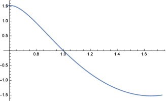
Figure 4.1: Figure of $\Phi(u)={\varphi}_{1}(u)-{\varphi}_{2}(u)$.

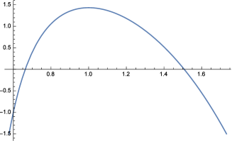
Figure 4.2: Figure of $\Psi(u)=\psi_{1}(u)-\psi_{2}(u)$.

4.2 The ${\omega}$-Maslov indices and instability in $[1/\sqrt{3},\sqrt{3}]\times[0,1)$

We first study the monotonicity of eigenvalues of ${\cal A}(u,e)$ and ${\cal B}(u,e)$ with respect to $u$. Together with the indices obtained in Section 3, we can obtain the indices of ${\cal A}(u,e)$ and ${\cal B}(u,e)$ for $(u,e)\in[1/\sqrt{3},\sqrt{3}]\times[0,1)$. We rewrite ${\cal A}(u,e)$ as follows:

$${\cal A}(u,e)=\begin{cases}({\varphi}_{1}-{\varphi}_{2})\bar{{\cal A}}(u,e),\ \mbox{ if }\ 1/\sqrt{3}\leq u<1;\\ ({\varphi}_{2}-{\varphi}_{1})\bar{{\cal A}}(u,e),\ \mbox{ if }\ 1<u\leq\sqrt{3},\end{cases}$$ (4.12)

where $\bar{{\cal A}}(u,e)$ is given by

$$\bar{{\cal A}}(u,e)=\begin{cases}\frac{{\cal A}(1,e)}{{\varphi}_{1}-{\varphi}_{2}}+\frac{S(t)}{2(1+e\cos t)},\;\mbox{{ if}}\;1/\sqrt{3}\leq u<1,\\ \frac{{\cal A}(1,e)}{{\varphi}_{2}-{\varphi}_{1}}-\frac{S(t)}{2(1+e\cos t)},\;\mbox{{ if}}\;1<u\leq\sqrt{3}.\end{cases}$$ (4.13)

By Lemma 4.3, $\Phi(u)={\varphi}_{1}(u)-{\varphi}_{2}(u)>0$ if $1/\sqrt{3}\leq u<1$ and $\Phi(u)<0$ if $1<u\leq\sqrt{3}$. Thus, $\phi_{{\omega}}({\cal A}(u,e))=\phi_{{\omega}}(\bar{{\cal A}}(u,e))$ and $\nu_{{\omega}}({\cal A}(u,e))=\nu_{{\omega}}(\bar{{\cal A}}(u,e))$. Accordingly, the index $\phi_{{\omega}}({\cal A}(u,e))$ can be obtained by computing $\phi_{{\omega}}(\bar{{\cal A}}(u,e))$. First, the monotonicity of $\phi_{{\omega}}(\bar{{\cal A}}(u,e))$ is given as follows.

Lemma 4.5.

• For each fixed $e\in[0,1)$ and any fixed $\omega\in{\bf U}$, the operator $\bar{{\cal A}}(u,e)$ is increasing in $u$ when $u\in(u_{1},1)\cup(1/u_{1},\sqrt{3})$ and is decreasing when $u\in(1/\sqrt{3},u_{1})\cup(1,1/u_{1})$ where $u_{1}$ is given in Lemma 4.3.

• For every eigenvalue ${\lambda}_{u_{0}}=0$ of $\bar{{\cal A}}(u_{0},e_{0})$ with ${\omega}\in{\bf U}$ for some $(u_{0},e_{0})\in[1/\sqrt{3},\sqrt{3}]\times[0,1)$, $\frac{{\mathrm{d}}}{{\mathrm{d}}u}{\lambda}_{u}|_{u=u_{0}}>0$ when $u_{0}\in(u_{1},1)\cup(1/u_{1},\sqrt{3}]$; and $\frac{{\mathrm{d}}}{{\mathrm{d}}u}{\lambda}_{u}|_{u=u_{0}}<0$ when $u_{0}\in[1/\sqrt{3},u_{1})\cup(1,1/u_{1})$.

Proof.

Via direct computations, we have $\frac{\partial}{\partial u}\bar{{\cal A}}(u,e)|_{u=u_{0}}=-\frac{{\cal A}(1,e)}{({\varphi}_{1}-{\varphi}_{2})^{2}}\frac{\partial\Phi}{\partial u}$ if $1/\sqrt{3}<u<1$, and $\frac{\partial}{\partial u}\bar{{\cal A}}(u,e)|_{u=u_{0}}=\frac{{\cal A}(1,e)}{({\varphi}_{2}-{\varphi}_{1})^{2}}\frac{\partial\Phi}{\partial u}$ if $1<u<\sqrt{3}.$ By the positive definiteness of ${\cal A}(1,e)$ in Theorem 3.2, both $\frac{{\cal A}(1,e)}{({\varphi}_{1}-{\varphi}_{2})^{2}}$ and $\frac{{\cal A}(1,e)}{({\varphi}_{2}-{\varphi}_{1})^{2}}$ are positive definite operators on $D({\omega},2\pi)$ for any ${\omega}\in{\bf U}$. By (3.2) and Lemma 4.3, $\frac{{\mathrm{d}}\Phi}{{\mathrm{d}}u}>0$ if $u\in(1/\sqrt{3},u_{1})\cup(1,1/u_{1})$, and $\frac{{\mathrm{d}}\Phi}{{\mathrm{d}}u}<0$ if $u\in(u_{1},1)\cup(1/u_{1},\sqrt{3})$. Therefore, we can determine that (i) of this lemma holds.

Let $x_{0}=x_{0}(t)$ with unit norm such that $\bar{{\cal A}}(u_{0},e_{0})x_{0}=0$. Fix $e_{0}$. Then, $\bar{{\cal A}}(u,e_{0})$ is an analytic path of strictly increasing self-adjoint operators with respect to $u$ if $u\in(u_{1},1)\cup(1/u_{1},\sqrt{3}]$ and is an analytic path of strictly decreasing self-adjoint operators with respect to $u$ if $u\in[1/\sqrt{3},u_{1})\cup(1,1/u_{1})$.

Following Kato ([7], p.120 and p.386), we can select a smooth path of unit norm eigenvectors $x_{u}$ with $x_{u_{0}}=x_{0}$ belonging to a smooth path of real eigenvalues ${\lambda}_{u}$ of the self-adjoint operator $\bar{{\cal A}}(u,e_{0})$ on $\overline{D}({\omega},2\pi)$ such that for small enough $|u-u_{0}|$, we have

$$\bar{{\cal A}}(u,e_{0})x_{u}=\lambda_{u}x_{u},$$ (4.14)

where $\lambda_{u_{0}}=0$. Taking inner product with $x_{u}$ on both sides of (4.14) and then differentiating it with respect to $u$ at $u_{0}$, we have

$$\frac{{\mathrm{d}}}{{\mathrm{d}}u}\lambda_{u}|_{u=u_{0}}= {\langle}\frac{\partial}{\partial u}\bar{A}(u,e_{0})x_{u},x_{u}{\rangle}|_{u=u_{0}}+2{\langle}\bar{A}(u,e_{0})x_{u},\frac{\partial}{\partial u}x_{u}{\rangle}|_{u=u_{0}}$$

$${=} \begin{cases}\frac{1}{({\varphi}_{1}-{\varphi}_{2})^{2}}\frac{\partial({\varphi}_{2}-{\varphi}_{1})}{\partial u}{\langle}{\cal A}(1,e)x_{0},x_{0}{\rangle},\quad\text{{ if}}\;1/\sqrt{3}<u<1,\\ \frac{1}{({\varphi}_{2}-{\varphi}_{1})^{2}}\frac{\partial({\varphi}_{1}-{\varphi}_{2})}{\partial u}{\langle}{\cal A}(1,e)x_{0},x_{0}{\rangle},\quad\text{{ if}}\;1<u<\sqrt{3},\end{cases}$$ (4.15)

where the last equality follows from the definition of $\bar{{\cal A}}(u,e)$. By (4.15) and the positive definiteness of ${\cal A}(1,e)$, $\frac{{\mathrm{d}}}{{\mathrm{d}}u}{\lambda}_{u}|_{u=u_{0}}>0$ if $u_{0}\in(u_{1},1)\cup(1/u_{1},\sqrt{3})$; and $\frac{{\mathrm{d}}}{{\mathrm{d}}u}{\lambda}_{u}|_{u=u_{0}}<0$ if $u_{0}\in(1/\sqrt{3},u_{1})\cup(1,1/u_{1})$. Thus, this lemma holds. ∎

Corollary 4.6.

For every given $e\in[0,1)$ and ${\omega}\in{\bf U}$, the index $\phi_{{\omega}}({\cal A}(u,e))$ is non-decreasing as $u$ increases from $u_{1}$ to $1$ and from $1/u_{1}$ to $\sqrt{3}$; and it is non-increasing as $u$ increases from $1/\sqrt{3}$ to $u_{1}$ and from $1$ to $1/u_{1}$. In particular, the index of $\phi_{{\omega}}({\cal A}(u,e))$ satisfies $\phi_{{\omega}}({\cal A}(u,e))\geq\phi_{{\omega}}({\cal A}(u_{1},e))$ for $u\in(1/\sqrt{3},1]$, and $\phi_{{\omega}}({\cal A}(u,e))\geq\phi_{{\omega}}({\cal A}(1/u_{1},e))$ for $u\in[1,\sqrt{3})$.

Proof.

For $u_{1}\leq u^{\prime}<u^{\prime\prime}<1$ and fixed $e\in[0,1)$, when $u$ increases from $u^{\prime}$ to $u^{\prime\prime}$, it is possible that the negative eigenvalues of $\bar{{\cal A}}(u^{\prime},e)$ pass through $0$ and become positive ones of $\bar{{\cal A}}(u^{\prime\prime},e)$; however, it is impossible that positive eigenvalues of $\bar{{\cal A}}(u^{\prime},e)$ pass through $0$ and become negative according to (ii) of Lemma 4.5. Similar arguments also hold if $u$ is in the intervals $(1/\sqrt{3},u_{1})$, $(1,1/u_{1})$, and $(1/u_{1},\sqrt{3})$. Therefore, this corollary holds. ∎

Next, we consider the ${\omega}$-Morse index and nullity of ${\cal A}(u,e)$ if $u=u_{1}$ and $u=1/u_{1}$.

Lemma 4.7.

• For any ${\omega}$ boundary condition, when $e\in[0,\hat{f}({\beta}_{1})^{-1/2})$, both the operators ${\cal A}(u_{1},e)$ and ${\cal A}(1/u_{1},e)$ are non-degenerate positive operators; i.e.,

  $$\phi_{{\omega}}({\cal A}(u_{1},e))=\phi_{{\omega}}({\cal A}(1/u_{1},e))=0,\;\nu_{{\omega}}({\cal A}(u_{1},e))=\nu_{{\omega}}({\cal A}(1/u_{1},e))=0.$$ (4.16)

• By the numerical results in [17], when $e\in[0,1)$, the results of (i) hold.

Proof.

Note that ${\cal A}(u_{1},e)$ is

$${\cal A}(u_{1},e)=-\frac{{\mathrm{d}}^{2}}{{\mathrm{d}}t^{2}}I_{2}-I_{2}+\frac{1}{2(1+e\cos t)}(({\varphi}_{1}(u_{1})+{\varphi}_{2}(u_{1}))I_{2}+({\varphi}_{1}(u_{1})-{\varphi}_{2}(u_{1}))S(t)).$$ (4.17)

where ${\varphi}_{1}(u_{1})+{\varphi}_{2}(u_{1})\approx 3.10002>3$ and ${\varphi}_{1}(u_{1})-{\varphi}_{2}(u_{1})\approx 1.52657$ by direct computations. Since $\frac{I_{2}}{2(1+e\cos t)}$ is a positive operator on $D({\omega},2\pi)$, we have

$${\cal A}(u_{1},e)>-\frac{{\mathrm{d}}^{2}}{{\mathrm{d}}t^{2}}I_{2}-I_{2}+\frac{1}{2(1+e\cos t)}(3I_{2}+({\varphi}_{1}(u_{1})-{\varphi}_{2}(u_{1}))S(t)).$$ (4.18)

Let ${\beta}_{1}:=9-({\varphi}_{1}(u_{1})-{\varphi}_{2}(u_{1}))^{2}.$ The numerical computations show that ${\beta}_{1}\approx 9-(1.52657)^{2}=6.66958$. By Theorem B.3, the $\zeta_{{\beta}_{1},e}(2\pi)$ is hyperbolic if $0\leq e<{\hat{f}({\beta}_{1})^{-1/2}}$ where $\hat{f}({\beta}_{1})$ is given by (B.10). It follows that the right-hand side of (4.18) is positive definite with zero nullity for any ${\omega}$ boundary condition. By (4.18), $\phi_{{\omega}}({\cal A}(u_{1},e))=0$, and $\nu_{{\omega}}({\cal A}(u_{1},e))=0$ for any ${\omega}\in{\bf U}$ and $0\leq e<\hat{f}({\beta}_{1})^{-1/2}$. By Proposition 3.1, it follows that $\phi_{{\omega}}({\cal A}(u_{1},e))=\phi_{{\omega}}({\cal A}(1/u_{1},e))$ and $\nu_{{\omega}}({\cal A}(u_{1},e))=\nu_{{\omega}}({\cal A}(1/u_{1},e))$. Therefore, we have (i) of this lemma.

The numerical results in [17] have shown that $\zeta_{{\beta}_{1},e}(2\pi)$ is hyperbolic. It follows that $\phi_{{\omega}}({\cal A}(u_{1},e))=0$ and $\nu_{{\omega}}({\cal A}(u_{1},e))=0$ for any $e\in[0,1)$ and ${\omega}\in{\bf U}$. It yields that (ii) of this lemma holds. ∎

The proof of Lemma 1.1 can be obtained directly, as follows.

Proof of Lemma 1.1.

By Theorem 3.3 and Lemma 4.7, we determine that Lemma 1.1 holds. ∎

Theorem 4.8.

• By (i) of Lemma 1.1, for any $(u,e)\in[1/\sqrt{3},\sqrt{3}]\times[0,\hat{f}({\beta}_{1})^{-1/2})$ and ${\omega}\in{\bf U}$, ${\cal A}(u,e)$ is a positive definite operator with zero nullity on the space $\overline{D}({\omega},2\pi)$; i.e., $\phi_{{\omega}}({\cal A}(u,e))=0$, and $\nu_{{\omega}}({\cal A}(u,e))=0.$

• By (ii) of Lemma 1.1, for any $(u,e)\in[1/\sqrt{3},\sqrt{3}]\times[0,1)$, the results of (i) hold.

Proof.

By Corollary 4.6, for any given $e\in[0,1)$, $\phi_{{\omega}}({\cal A}(u,e))\geq\phi_{{\omega}}({\cal A}(u_{1},e))>0$ when $u\in(1/\sqrt{3},1]$ and $\phi_{{\omega}}({\cal A}(u,e))\geq\phi_{{\omega}}({\cal A}(1/u_{1},e))>0$ when $u\in[1,\sqrt{3})$. By (i) of Lemma 4.7, for any $(u,e)\in[1/\sqrt{3},\sqrt{3}]\times[0,\hat{f}({\beta}_{1})^{-1/2})$, we have that $\phi_{{\omega}}({\cal A}(u,e))=0$ and $\nu_{{\omega}}({\cal A}(u,e))=0$. Then (i) of this theorem holds.

By (ii) of Lemma 4.7, we can obtain (ii) of this theorem holds, following the same argument. ∎

Remark 4.9.

As demonstrated by the discussion in Section 3, ${\cal A}(1,e)$ is a positive definite operator for $e\in[0,1)$. By the continuity of eigenvalues of ${\cal A}(1,e)$, there exists a $u_{*}\in(1/\sqrt{3},1)$ such that when $(u,e)\in(u_{*},1/u_{*})\times[0,1)$, ${\cal A}(u,e)$ is a positive definite operator with zero nullity.

We next study the operator ${\cal B}(u,e)$ following similar arguments as ${\cal A}(u,e)$. Since $\psi_{1}(u)=\psi_{1}(1/u)$ and $\psi_{2}(u)=\psi_{2}(1/u)$, we have ${\cal B}(u,e)={\cal B}(1/u,e)$ for $(u,e)\in[1/\sqrt{3},\sqrt{3}]\times[0,1)$. Therefore, we restrict our attention to $(u,e)\in[1/\sqrt{3},1]\times[0,1)$.

Via direct computations, we obtain that $\psi_{1}(u)+\psi_{2}(u)=3$ for any $u\in[1/\sqrt{3},\sqrt{3}]$. By Lemma 4.4, $\Psi(u_{2})=\psi_{1}(u_{2})-\psi_{2}(u_{2})=0$. It follows that ${\cal B}(u_{2},e)$ is given by the following:

$${\cal B}(u_{2},e)=-\frac{{\mathrm{d}}^{2}}{{\mathrm{d}}t^{2}}I_{2}-I_{2}+\frac{3}{2(1+e\cos t)}.$$ (4.19)

By Corollary 4.3 of [3], ${\cal B}(u_{2},e)$ is a positive definite operator with zero nullity for any ${\omega}$ boundary. We rewrite ${\cal B}(u,e)$ in (2.33) as follows:

$${\cal B}(u,e)=\begin{cases}(\psi_{2}-\psi_{1})\bar{{\cal B}}(u,e),\ \mbox{ if }\ 1/\sqrt{3}<u<u_{2},\\ (\psi_{1}-\psi_{2})\bar{{\cal B}}(u,e),\ \mbox{ if }\ u_{2}<u<1,\end{cases}$$ (4.20)

where $\bar{{\cal B}}(u,e)$ is given by

$$\bar{{\cal B}}(u,e)=\begin{cases}\frac{{\cal B}(u_{2},e)}{\psi_{2}-\psi_{1}}-\frac{S(t)}{2(1+e\cos t)},\;\mbox{{if}}\;1/\sqrt{3}<u<u_{2},\\ \frac{{\cal B}(u_{2},e)}{\psi_{1}-\psi_{2}}+\frac{S(t)}{2(1+e\cos t)},\;\mbox{{if}}\;u_{2}<u<1.\end{cases}$$ (4.21)

Then, $\frac{\partial}{\partial u}\bar{{\cal B}}(u,e)|_{u=u_{0}}=\frac{{\cal B}(u_{2},e)}{(\psi_{2}-\psi_{1})^{2}}\frac{{\mathrm{d}}\Psi}{{\mathrm{d}}u}$ if $1/\sqrt{3}\leq u<u_{2}$, and $\frac{\partial}{\partial u}\bar{{\cal B}}(u,e)|_{u=u_{0}}=-\frac{{\cal B}(u_{2},e)}{(\psi_{1}-\psi_{2})^{2}}\frac{{\mathrm{d}}\Psi}{{\mathrm{d}}u}$ if $u_{2}<u\leq 1$. By Lemma 4.4, we use a similar argument as in Lemma 4.5 and obtain the following lemma and corollary.

Lemma 4.10.

• For each fixed $e\in[0,1)$, the operator $\bar{{\cal B}}(u,e)$ is increasing when $u\in[1/\sqrt{3},u_{2})$ and is decreasing when $u\in(u_{2},1)$.

• For every eigenvalue ${\lambda}_{u_{0}}=0$ of $\bar{{\cal B}}(u_{0},e_{0})$ with ${\omega}\in{\bf U}$ for some $(u_{0},e_{0})\in(1/\sqrt{3},1)\times[0,1)$, $\frac{{\mathrm{d}}}{{\mathrm{d}}u}{\lambda}_{u}|_{u=u_{0}}>0$, if $u_{0}\in(1/\sqrt{3},u_{2})$ and $\frac{{\mathrm{d}}}{{\mathrm{d}}u}{\lambda}_{u}|_{u=u_{0}}<0$ if $u_{0}\in(u_{2},1)$.

Corollary 4.11.

For every fixed $e\in[0,1)$ and ${\omega}\in{\bf U}$, the index $\phi_{{\omega}}({\cal B}(u,e))$ is non-decreasing as $u$ increases from $1/\sqrt{3}$ to $u_{2}$ and is non-increasing as $u$ increases from $u_{2}$ to $1$. In particular, the index $\phi_{{\omega}}({\cal B}(u,e))$ satisfies $\phi_{{\omega}}({\cal B}(u,e))\geq\phi_{{\omega}}({\cal B}(1/\sqrt{3},e))$ when $u\in[1/\sqrt{3},u_{2})\cup(1/u_{2},\sqrt{3}]$ and $\phi_{{\omega}}({\cal B}(u,e))\geq\phi_{{\omega}}({\cal B}(1,e))$, when $u\in[u_{2},{1/u_{2}}]$.

Theorem 4.12.

• By (i) of Lemma 1.1, for any $(u,e)\in[1/\sqrt{3},u_{2})\times[0,\hat{f}(\frac{27}{4})^{-1/2})\cup[u_{2},1/u_{2}]\times[0,1)\cup(1/u_{2},\sqrt{3}]\times[0,\hat{f}(\frac{27}{4})^{-1/2})$, the operator ${\cal B}(u,e)$ is positive definite with zero nullity on the space $\overline{D}(2\pi,{\omega})$; i.e.,

  $$\phi_{{\omega}}({\cal B}(u,e))=0,\;\nu_{{\omega}}({\cal B}(u,e))=0.$$ (4.22)

• By (ii) of Lemma 1.1, when $(u,e)\in[1/\sqrt{3},\sqrt{3}]\times[0,1)$, the results of (i) hold.

Since the proof of Theorem 4.12 is similar to that of Theorem 4.8, we sketch the proof below.

Sketch of proof..

By Theorem 3.3 and Corollary 4.11, we have that (4.22) holds when $(u,e)\in[1/\sqrt{3},u_{2})\times[0,\hat{f}(\frac{27}{4})^{-1/2})\cup[u_{2},1/u_{2}]\times[0,1)\cup(1/u_{2},\sqrt{3}]\times[0,\hat{f}(\frac{27}{4})^{-1/2})$. By Theorem 3.2 and Corollary 4.11, (4.22) holds when $(u,e)\in[u_{2},1/u_{2}]\times[0,1)$. This shows that (i) of this theorem holds.

By Corollary 4.11, Theorem 3.2 and (ii) of Theorem 3.3, (4.22) holds when $(u,e)\in[1/\sqrt{3},\sqrt{3}]\times[0,1)$. Thus, (ii) of this theorem holds. ∎

Proof of Theorem 1.2..

By Lemma 2.4, we have that $i_{{\omega}}({\gamma}_{u,e})=\phi_{{\omega}}({\cal A}(u,e))$ and $\nu_{{\omega}}({\gamma}_{u,e})=\nu_{{\omega}}({\cal A}(u,e))$. By Theorem 4.8, we have for $(u,e)\in[1/\sqrt{3},\sqrt{3}]\times[0,\hat{f}({\beta}_{1})^{-1/2})$, $i_{{\omega}}({\gamma}_{u,e})=0$ and $\nu_{{\omega}}({\gamma}_{u,e})=0$ . By [13] (cf. pp. 179–183) and the proof of Theorem 1.4 in [3], all eigenvalues of the matrix ${\gamma}_{u,e}(2\pi)$ are hyperbolic; i.e., all eigenvalues are not on ${\bf U}$.

Again, by Lemma 2.4 and Theorem 4.12, it follows that $i_{{\omega}}(\eta_{u,e})=\phi_{{\omega}}({\cal B}(u,e))=0$ and $\nu_{{\omega}}(\eta_{u,e})=\nu_{{\omega}}({\cal B}(u,e))=0$ for $(u,e)\in[1/\sqrt{3},u_{2})\times[0,\hat{f}(\frac{27}{4})^{-1/2})\cup[u_{2},1/u_{2}]\times[0,1)\cup(1/u_{2},\sqrt{3}]\times[0,\hat{f}(\frac{27}{4})^{-1/2})$. Therefore, when $(u,e)\in[1/\sqrt{3},u_{2})\times[0,\hat{f}(\frac{27}{4})^{-1/2})\cup[u_{2},1/u_{2}]\times[0,1)\cup(1/u_{2},\sqrt{3}]\times[0,\hat{f}(\frac{27}{4})^{-1/2})$, all eigenvalues of $\eta_{u,e}(2\pi)$ are hyperbolic; i.e., all eigenvalues are not on ${\bf U}$.

The fundamental solution ${\gamma}_{0}(2\pi)$ of (2.18) satisfies ${\gamma}_{0}(2\pi)={\gamma}_{1}(2\pi)\diamond{\gamma}_{u,e}(2\pi)\diamond\eta_{u,e}(2\pi).$ Since ${\gamma}_{1}(2\pi)$ is elliptic with ${\gamma}_{1}(2\pi)=I_{2}\diamond N_{1}(1,1)$, we can determine that ${\gamma}_{0}(2\pi)$ is hyperbolic if ${\gamma}_{u,e}(2\pi)$ or $\eta_{u,e}(2\pi)$ is hyperbolic.

Note that $\hat{f}(\frac{27}{4})^{-1/2}>\hat{f}({\beta}_{1})^{-1/2}$ by (B.10). We have ${\gamma}_{u,e}(2\pi)$ possesses at least one pair of hyperbolic eigenvalues $(u,e)\in(1/\sqrt{3},u_{2})\times[0,\hat{f}(\frac{27}{4})^{-1/2})\cup(u_{2},1/u_{2})\times[0,1)\cup(1/u_{2},\sqrt{3})\times[0,\hat{f}(\frac{27}{4})^{-1/2})$. Thus, (i) of Theorem 1.2 holds.

By (ii) of Theorem 4.8 and (ii) of Theorem 4.12, both ${\gamma}_{u,e}(2\pi)$ and $\eta_{u,e}(2\pi)$ possess two pairs of hyperbolic eigenvalues for $(u,e)\in(1/\sqrt{3},\sqrt{3})\times[0,1)$. Following the same argument given above, we can determine that ${\gamma}_{0}(2\pi)$ possesses four pairs of hyperbolic eigenvalues when $(u,e)\in[1/\sqrt{3},\sqrt{3}]\times[0,1)$ by (ii) of Theorem 4.8 and (ii) of Theorem 4.12. ∎

Appendix

Appendix A The $\omega$-Maslov Indices and $\omega$-Morse Indices

Let $({\bf R}^{2n},\Omega)$ be the standard symplectic vector space with coordinates $(x_{1},...,x_{n}$, $y_{1},...,y_{n})$ and the symplectic form $\Omega=\sum_{i=1}^{n}dx_{i}\wedge dy_{i}$. Let $J=(\begin{smallmatrix}0&-I_{n}\\ I_{n}&0\end{smallmatrix})$ be the standard symplectic matrix, where $I_{n}$ is the identity matrix on ${\bf R}^{n}$. Given any two $2m_{k}\times 2m_{k}$ matrices of square block form $M_{k}=(\begin{smallmatrix}A_{k}&B_{k}\\ C_{k}&D_{k}\end{smallmatrix})$ with $k=1,2$, the symplectic sum of $M_{1}$ and $M_{2}$ is defined (cf. [11] and [13]) by the following $2(m_{1}+m_{2})\times 2(m_{1}+m_{2})$ matrix $M_{1}{\diamond}M_{2}$:

$$M_{1}{\diamond}M_{2}=\begin{pmatrix}A_{1}&0&B_{1}&0\\ 0&A_{2}&0&B_{2}\\ C_{1}&0&D_{1}&0\\ 0&C_{2}&0&D_{2}\end{pmatrix}.$$ (A.1)

For any two paths ${\gamma}_{j}\in{\cal P}_{\tau}(2n_{j})$ with $j=0$ and $1$, let ${\gamma}_{0}{\diamond}{\gamma}_{1}(t)={\gamma}_{0}(t){\diamond}{\gamma}_{1}(t)$ for all $t\in[0,\tau]$.

It is well known that that the fundamental solution ${\gamma}(t)$ of the linear Hamiltonian system with continuous symmetric periodic coefficients is a path in the symplectic matrix group ${\rm Sp}(2n)$, starting from the identity. In the Lagrangian case, when $n=2$, the Maslov-type index $i_{{\omega}}({\gamma})$ is defined by the usual homotopy intersection number about the hypersurface ${\rm Sp}(2n)^{0}=\{M\in{\rm Sp}(2n)\,|\,D_{{\omega}}(M)=0\}$ where $D_{{\omega}}(M)=(-1)^{n-1}\overline{{\omega}}^{n}\det(M-{\omega}I_{2n})$. Moreover, the nullity is defined by $\nu_{{\omega}}(M)=\dim_{{\bf C}}\ker_{{\bf C}}({\gamma}(2\pi)-{\omega}I_{2n})$. Please refer to [11, 12, 13] for more details on this index theory of symplectic matrix paths and periodic solutions of Hamiltonian systems.

For $T>0$, suppose that $x$ is a critical point of the functional

$$F(x)=\int_{0}^{T}L(t,x,\dot{x})dt,\qquad\forall\,\,x\in W^{1,2}({\bf R}/T{\bf Z},{\bf R}^{n}),$$

where $L\in C^{2}(({\bf R}/T{\bf Z})\times{\bf R}^{2n},{\bf R})$ and satisfies the Legendrian convexity condition $L_{p,p}(t,x,p)>0$. It is well known that $x$ satisfies the corresponding Euler-Lagrangian equation:

$$\frac{d}{dt}L_{p}(t,x,\dot{x})-L_{x}(t,x,\dot{x})=0,$$ (A.2)

$$x(0)=x(T),\qquad\dot{x}(0)=\dot{x}(T).$$ (A.3)

For such an extremal loop, define $P(t)=L_{p,p}(t,x(t),\dot{x}(t))$, $Q(t)=L_{x,p}(t,x(t),\dot{x}(t))$, $R(t)=L_{x,x}(t,x(t),\dot{x}(t))$. Note that $F\,^{\prime\prime}(x)=-\frac{d}{dt}(P\frac{d}{dt}+Q)+Q^{T}\frac{d}{dt}+R.$

For $\omega\in{\bf U}$, set $D(\omega,T)=\{y\in W^{1,2}([0,T],{\bf C}^{n})\,|\,y(T)=\omega y(0)\}.$ We define the $\omega$-Morse index $\phi_{\omega}(x)$ of $x$ to be the dimension of the largest negative definite subspace of $\langle F\,^{\prime\prime}(x)y_{1},y_{2}\rangle$, for all $y_{1},y_{2}\in D(\omega,T)$, where $\langle\cdot,\cdot\rangle$ is the inner product in $L^{2}$. For $\omega\in{\bf U}$, we also set $\overline{D}(\omega,T)=\{y\in W^{2,2}([0,T],{\bf C}^{n})\,|\,y(T)=\omega y(0),\dot{y}(T)={\omega}\dot{y}(0)\}.$ Then $F^{\prime\prime}(x)$ is a self-adjoint operator on $L^{2}([0,T],{\bf R}^{n})$ with domain $\overline{D}(\omega,T)$. We also define the nullity $\nu_{\omega}(x)$ by $\nu_{\omega}(x)=\dim\ker(F^{\prime\prime}(x))$.

On the other hand, $\tilde{x}(t)=(\partial L/\partial\dot{x}(t),x(t))^{T}$ is the solution of the corresponding Hamiltonian system of (A.2)-(A.3); moreover, its fundamental solution $\gamma(t)$ is given by $\dot{\gamma}(t)=JB(t)\gamma(t)$, where $\gamma(0)=I_{2n}$ and with $B(t)=(\begin{smallmatrix}P^{-1}(t)&-P^{-1}(t)Q(t)\\ -Q(t)^{T}P^{-1}(t)&Q(t)^{T}P^{-1}(t)Q(t)-R(t)\end{smallmatrix})$.

Lemma A.1 ([13], p.172).

For the $\omega$-Morse index $\phi_{\omega}(x)$ and nullity $\nu_{\omega}(x)$ of the solution $x=x(t)$ and the $\omega$-Maslov-type index $i_{\omega}(\gamma)$ and nullity $\nu_{\omega}(\gamma)$ of the symplectic path ${\gamma}$ corresponding to $\tilde{x}$, for any $\omega\in{\bf U}$ we have $\phi_{\omega}(x)=i_{\omega}(\gamma)$, and $\nu_{\omega}(x)=\nu_{\omega}(\gamma)$.

Appendix B A Brief Review of the Trace Formula.

In this section, we briefly review the trace formula introduced in [5]. Suppose that $Sym(k)$ represents the set of $k\times k$ real symmetric matrices. We consider the eigenvalue problem of Hamiltonian systems with periodical boundary condition as following.

$$\dot{z}(t)=J(B(t)+\lambda D(t))z(t),\quad z(0)=z(2\pi),$$ (B.1)

where $B(t),D(t)\in C([0.2\pi],Sym(k))$. Let ${A}=-J\frac{{\mathrm{d}}}{{\mathrm{d}}t}$, which is defined on a dense set of $E=L^{2}([0,T])$ with the domain $D_{S}=\left\{z(t)\in W^{1,2}\left([0,T];\mathbb{C}^{2n}\right)|z(0)=z(T)\right\}$. Note that the operator $A$ is self-adjoint with compact resolvent. For ${\lambda}\in\rho(A)$, the resolvent set of $A$, $({\lambda}-{A})^{-1}$ is Hilbert-Schmidt.

Suppose ${\gamma}_{{\lambda}}(t)$ is the fundamental solution of (B.1). To obtain the trace formula, we first define that $\hat{D}(t)={\gamma}_{0}^{T}(t)D(t){\gamma}_{0}(t)$. For $k\in{\bf N}$, let $M_{k}=\int^{2\pi}_{0}J\hat{D}(t_{1})\int^{t_{1}}_{0}J\hat{D}(t_{2})\cdots\int^{t_{k-1}}_{0}J\hat{D}(t_{k}){\mathrm{d}}t_{k}\cdots{\mathrm{d}}t_{2}{\mathrm{d}}t_{1}$, $\mathcal{M}(v)=M\left(M-\mathrm{e}^{vT}I_{2n}\right)^{-1}$, and $G_{k}(v)=M_{k}\cdot\mathcal{M}(v)$. Moreover, for $\nu\in{\bf C}$, $A-B-\nu J$ is invertible. Let $\mathcal{F}(v,B,D)=D(A-B-vJ)^{-1}$.

For the sake of simplicity, we abbreviate $\mathcal{F}(v,B,D)$ as $\mathcal{F}$. For $m\geq 2$, $\mathcal{F}_{m}$ are trace class operators. Note that ${\lambda}$ is a non-zero eigenvalue of system (B.1) if and only if $1/{\lambda}$ is an eigenvalue of $\mathcal{F}$. Therefore, if the sequence $\{{\lambda}_{i}\}$ is the set of non-zero eigenvalues of the system (B.1), $\operatorname{Tr}\left(\mathcal{F}^{m}\right)=\sum_{j}\frac{1}{\lambda_{j}^{m}},$ where the sum is taken for all eigenvalues ${\lambda}_{j}$ of $\mathcal{F}$ with counting the algebraic multiplicity.

Theorem B.1 (Theorem 1.1 and Corollary 1.3 of [5]).

We have

$$\operatorname{Tr}\left(\mathcal{F}^{2}\right)=\operatorname{Tr}\left[\left(M_{1}\mathcal{M}(\nu)\right)^{2}-2M_{2}\mathcal{M}(\nu)\right].$$

We define $D_{\beta,e}(t)=B_{\beta,e}(t)-B_{\beta,0}(t)=\frac{e\cos(t)}{1+e\cos(t)}K_{\beta}$ where $K_{{\beta}}={\rm diag}(\frac{3+\sqrt{9+{\beta}}}{2},\frac{3-\sqrt{9+{\beta}}}{2})$. Then, $A-B_{{\beta},e}=A-B_{{\beta},0}-D_{{\beta},e}$. Let $\cos^{\pm}(t)=(\cos(t)\pm|\cos(t)|/2)$ and denote $K_{\beta}^{\pm}=\cos^{\pm}(t)K_{\beta}$. These can be considered as two bounded self-adjoint operators by $A-\nu J-B_{\beta,0}-\frac{e}{1-e}K_{\beta}^{-}\geq A-\nu J-B_{\beta,e}\geq A-\nu J-B_{\beta,0}-eK_{\beta}^{+},$ where $\nu$ is a pure imaginary number. Equivalently, we have

$$\mathcal{A}(\beta,0,v)-\frac{e}{1-e}\cos^{-}(t)\hat{K}_{\beta,0}\geq\mathcal{A}(\beta,e,v)\geq\mathcal{A}(\beta,0,v)-e\cos^{+}(t)\hat{K}_{\beta,0}.$$ (B.2)

Lemma B.2 (Lemma 5.2 of [5]).

For an imaginary number $\nu$, such that $A-\nu J-B_{{\beta},0}$ is invertible, we have $\operatorname{Tr}\left[\mathcal{F}\left(\nu,B_{\beta,0},K_{\beta}^{+}\right)^{2}\right]=\operatorname{Tr}\left[\mathcal{F}\left(\nu,B_{\beta,0},K_{\beta}^{-}\right)^{2}\right]$.

Denote $f(\beta,\omega)=\operatorname{Tr}\left[\mathcal{F}\left({\nu},B_{\beta,0},K_{\beta}^{-}\right)^{2}\right]=\operatorname{Tr}\left(\mathcal{F}\left({\nu},B_{\beta,0},K_{\beta}^{+}\right)^{2}\right)$ which is a positive function. Via the trace formula, the linear stability of the Hamiltonian system $\zeta_{{\beta},e}$ is given in the following theorem, where $\zeta_{{\beta},e}$ is the solution of

$$\zeta_{{\beta},e}^{\prime}= J\begin{pmatrix}1&0&0&1\\ 0&1&-1&0\\ 0&-1&\frac{2e\cos t-1-\sqrt{9-\beta}}{2(1+e\cos t)}&0\\ 1&0&0&\frac{2e\cos t-1+\sqrt{9-\beta}}{2(1+e\cos t)}\end{pmatrix}\zeta_{{\beta},e}.$$ (B.3)

Theorem B.3 (Theorem 5.6 of [5]).

For ${\beta}\in(1,9]$, $\zeta_{{\beta},e}(2\pi)$ in (B.3) is hyperbolic if $0\leq e<\hat{f}({\beta})^{-1/2}$ where $\hat{f}(\beta)=\sup\{f(\beta,\omega),\omega\in{\bf U}\}$.

In our discussion, we only concern about the case of ${\beta}=\frac{27}{4}$. Then, By the Section 5.3 of [5], we can given the expression of $\hat{f}(\frac{27}{4})$. By letting ${\beta}=\frac{27}{4}$ and direct computations, we have Let

$$f(\beta,\omega)=\operatorname{Tr}\left(\mathcal{F}\left(v,B_{\beta,0},K_{\beta}^{-}\right)^{2}\right)=2f_{1}(\beta,\omega)-f_{2}(\beta,\omega),$$ (B.4)

where

$$f_{1}=\frac{1}{4}\sum_{m,n=1}^{4}\frac{\exp(2\pi i{\theta}_{n})P_{nm}P_{mn}\left(2\exp(\pi i({\theta}_{m}-{\theta}_{n}))+i\pi\left(({\theta}_{m}-{\theta}_{n})^{2}-1\right)({\theta}_{m}-{\theta}_{n})+2\right)}{\left(2\left(({\theta}_{m}-{\theta}_{n})^{2}-1\right)^{2}\right)(\exp(2\pi i{\theta}_{n})-\exp(2\pi iu))},$$

and

$$f_{2}=\frac{1}{4}\sum_{m,n=1}^{4}\frac{\exp(2\pi i{\theta}_{m})\exp(2\pi i{\theta}_{n})P_{nm}P_{mn}(\exp(-\pi i({\theta}_{m}-{\theta}_{n}))+\exp(\pi i({\theta}_{m}-{\theta}_{n}))+2)}{\left(({\theta}_{m}-{\theta}_{n})^{2}-1\right)^{2}(\exp(2\pi i{\theta}_{m})-\exp(2\pi iu))(\exp(2\pi i{\theta}_{n})-\exp(2\pi iu))},$$ (B.6)

with ${\theta}=\left(-\sqrt{\frac{1}{2}\left(1-\frac{i\sqrt{23}}{2}\right)},\sqrt{\frac{1}{2}\left(1+\frac{i\sqrt{23}}{2}\right)},\sqrt{\frac{1}{2}\left(1-\frac{i\sqrt{23}}{2}\right)},-\sqrt{\frac{1}{2}\left(1+\frac{i\sqrt{23}}{2}\right)}\right)$ and

$$P= (P_{mn})_{4\times 4}$$

$$= \left(\begin{array}[]{cccc}\frac{3i\sqrt{\frac{2}{23}-\frac{i}{\sqrt{23}}}\left(21i+\sqrt{23}\right)}{2\left(5i+\sqrt{23}\right)}&-\frac{3\sqrt[4]{3}\left(-1+\sqrt{3}\right)}{\sqrt{23}}&\frac{3i}{2}\sqrt{\frac{2}{23}-\frac{i}{\sqrt{23}}}&\frac{3\sqrt[4]{3}\left(1+\sqrt{3}\right)}{\sqrt{23}}\\ \frac{3\sqrt[4]{3}\left(-1+\sqrt{3}\right)}{\sqrt{23}}&\frac{3\sqrt{\frac{2}{23}+\frac{i}{\sqrt{23}}}\left(21+i\sqrt{23}\right)}{2\left(-5i+\sqrt{23}\right)}&\frac{3\sqrt[4]{3}\left(1+\sqrt{3}\right)}{\sqrt{23}}&\frac{-3i}{2}\sqrt{\frac{2}{23}+\frac{i}{\sqrt{23}}}\\ \frac{-3i}{2}\sqrt{\frac{2}{23}-\frac{i}{\sqrt{23}}}&\frac{3\sqrt[4]{3}\left(1+\sqrt{3}\right)}{\sqrt{23}}&\frac{3\sqrt{\frac{2}{23}-\frac{i}{\sqrt{23}}}\left(21-i\sqrt{23}\right)}{2\left(5i+\sqrt{23}\right)}&-\frac{3\sqrt[4]{3}\left(-1+\sqrt{3}\right)}{\sqrt{23}}\\ \frac{3\sqrt[4]{3}\left(1+\sqrt{3}\right)}{\sqrt{23}}&\frac{3i}{2}\sqrt{\frac{2}{23}+\frac{i}{\sqrt{23}}}&\frac{3\sqrt[4]{3}\left(-1+\sqrt{3}\right)}{\sqrt{23}}&-\frac{3i\sqrt{\frac{2}{23}+\frac{i}{\sqrt{23}}}\left(-21i+\sqrt{23}\right)}{2\left(-5i+\sqrt{23}\right)}\end{array}\right).$$

By the numerical computations of Mathematica, we have $\hat{f}(\frac{27}{4})=\sup\left\{f(\frac{27}{4},\omega),\omega\in{\bf U}\right\}\approx 5.03999$ and $\hat{f}({\beta}_{1})=\sup\left\{f({\beta}_{1},\omega),\omega\in{\bf U}\right\}\approx 5.08507$. It follows that

$$\hat{f}(\frac{27}{4})^{-\frac{1}{2}}\approx 0.4454,\;{\mbox{and}\;\hat{f}({\beta}_{1})^{-\frac{1}{2}}\approx 0.4435.}$$ (B.10)

Appendix C Necessary computations

C.1 Computations in reduction

By (2.3)-(2.6), (2.8) and direct computations, we have the following equations hold.

$$A^{T}_{13}B_{11}A_{13} =A^{T}_{33}B_{33}A_{33}=\frac{{\alpha}^{3}}{(m+1)(1+u^{2})^{5/2}}\left(\begin{matrix}2-u^{2}&0\\ 0&2u^{2}-1\end{matrix}\right)+\frac{{\alpha}^{3}m}{16u^{3}(m+1)}\begin{pmatrix}-1&0\\ 0&2\end{pmatrix},$$ (C.1)

$$A^{T}_{23}B_{22}A_{23} =A^{T}_{43}B_{44}A_{43}=\frac{{\alpha}^{3}m^{2}}{(m+1)(1+u^{2})^{5/2}}\left(\begin{matrix}2-u^{2}&0\\ 0&2u^{2}-1\end{matrix}\right)+\frac{{\alpha}^{3}m}{16(m+1)}\left(\begin{matrix}2&0\\ 0&-1\end{matrix}\right),$$ (C.2)

$$A^{T}_{33}B_{31}A_{13} =A^{T}_{13}B_{13}A_{33}=\frac{{\alpha}^{3}m}{16u^{3}(m+1)}\begin{pmatrix}1&0\\ 0&-2\end{pmatrix},$$ (C.3)

$$A^{T}_{23}B_{24}A_{43} =A^{T}_{43}B_{42}A_{23}=\frac{{\alpha}^{3}m}{16(m+1)}\begin{pmatrix}-2&0\\ 0&1\end{pmatrix},$$ (C.4)

$$A^{T}_{13}B_{12}A_{23} =A^{T}_{23}B_{21}A_{13}=A^{T}_{33}B_{34}A_{43}=A^{T}_{43}B_{43}A_{33}=\frac{-{\alpha}^{3}m}{(2m+2)(1+u^{2})^{5/2}}\begin{pmatrix}u^{2}-2&3u\\ 3u&1-2u^{2}\end{pmatrix},$$ (C.5)

$$A^{T}_{13}B_{14}A_{43} =A^{T}_{23}B_{23}A_{33}=A^{T}_{33}B_{32}A_{23}=A^{T}_{43}B_{41}A_{13}=\frac{-{\alpha}^{3}m}{(2m+2)(1+u^{2})^{5/2}}\begin{pmatrix}u^{2}-2&-3u\\ -3u&1-2u^{2}\end{pmatrix}.$$ (C.6)

Therefore, ${\sigma^{3}}\left.\frac{\partial^{2}U}{\partial w_{3}^{2}}\right|_{\xi_{0}}$ is given by

$${\sigma^{3}}\left.\frac{\partial^{2}U}{\partial w_{3}^{2}}\right|_{\xi_{0}}=\sum_{i=1}^{4}\sum_{j=1}^{4}A_{i3}^{T}B_{ij}A_{j3}=\frac{2(m+1){\alpha}^{3}}{(1+u^{2})^{5/2}}\begin{pmatrix}2-u^{2}&0\\ 0&2u^{2}-1\end{pmatrix}.$$ (C.7)

By (2.3)-(2.6), and (2.8), we have that $A^{T}_{14}B_{11}A_{13}=-A^{T}_{34}B_{33}A_{33}$, $A^{T}_{24}B_{22}A_{23}=-A^{T}_{44}B_{44}A_{43}$, $A^{T}_{34}B_{31}A_{13}=-A^{T}_{14}B_{13}A_{33}$, $A^{T}_{24}B_{24}A_{43}=-A^{T}_{44}B_{42}A_{23}$, $A^{T}_{24}B_{21}A_{13}=-A^{T}_{44}B_{43}A_{33}$, $A^{T}_{14}B_{12}A_{23}=-A^{T}_{34}B_{34}A_{43}$, $A^{T}_{44}B_{41}A_{13}=-A^{T}_{24}B_{23}A_{33}$, and $A^{T}_{34}B_{32}A_{23}=-A^{T}_{14}B_{14}A_{43}$. Therefore, $\frac{\partial^{2}U}{\partial w_{3}\partial w_{4}}$ is given by

$$\left.\frac{\partial^{2}U}{\partial w_{3}\partial w_{4}}\right|_{\xi_{0}}=\frac{1}{\sigma^{3}}\sum_{i=1}^{4}\sum_{j=1}^{4}A_{i4}^{T}B_{ij}A_{j3}=0.$$ (C.8)

By (2.3)-(2.6), and (2.8), we have that

$$A^{T}_{14}B_{11}A_{14}= A^{T}_{34}B_{33}A_{34}=\frac{2{\alpha}}{(1+u^{2})^{5/2}}\begin{pmatrix}2-u^{2}&0\\ 0&2u^{2}-1\end{pmatrix}+\frac{{\alpha}m}{8u^{3}}\begin{pmatrix}-1&0\\ 0&2\end{pmatrix},$$ (C.9)

$$A^{T}_{24}B_{22}A_{24}= A^{T}_{44}B_{44}A_{44}=\frac{2{\alpha}m^{2}u^{2}}{(1+u^{2})^{5/2}}\begin{pmatrix}2u^{2}-1&0\\ 0&2-u^{2}\end{pmatrix}+\frac{{\alpha}mu^{2}}{8}\begin{pmatrix}-1&0\\ 0&2\end{pmatrix},$$ (C.10)

$$A^{T}_{34}B_{31}A_{14}= A^{T}_{14}B_{13}A_{34}=\frac{{\alpha}m}{8u^{3}}\begin{pmatrix}-1&0\\ 0&2\end{pmatrix},$$ (C.11)

$$A^{T}_{24}B_{24}A_{44}= A^{T}_{44}B_{42}A_{24}=\frac{{\alpha}mu^{2}}{8}\begin{pmatrix}-1&0\\ 0&2\end{pmatrix},$$ (C.12)

$$A^{T}_{24}B_{21}A_{14}= A^{T}_{44}B_{43}A_{34}=\frac{{\alpha}mu}{(1+u^{2})^{5/2}}\begin{pmatrix}3u&1-2u^{2}\\ 2-u^{2}&-3u\end{pmatrix},$$ (C.13)

$$A^{T}_{14}B_{12}A_{24}= A^{T}_{34}B_{34}A_{44}=\frac{{\alpha}mu}{(1+u^{2})^{5/2}}\begin{pmatrix}3u&2-u^{2}\\ 1-2u^{2}&-3u\end{pmatrix},$$ (C.14)

$$A^{T}_{44}B_{41}A_{14}= A^{T}_{24}B_{23}A_{34}=\frac{{\alpha}mu}{(1+u^{2})^{5/2}}\begin{pmatrix}3u&2u^{2}-1\\ u^{2}-2&-3u\end{pmatrix},$$ (C.15)

$$A^{T}_{34}B_{32}A_{24}= A^{T}_{14}B_{14}A_{44}=\frac{{\alpha}mu}{(1+u^{2})^{5/2}}\begin{pmatrix}3u&u^{2}-2\\ 2u^{2}-1&-3u\end{pmatrix}.$$ (C.16)

Therefore, it follows that $\left.\frac{\partial^{2}U}{\partial w_{4}^{2}}\right|_{\xi_{0}}$ can be calculated as follows.

$$\left.\frac{\partial^{2}U}{\partial w_{4}^{2}}\right|_{\xi_{0}}=\frac{1}{\sigma^{3}}\sum_{i=1}^{4}\sum_{j=1}^{4}A_{i4}^{T}B_{ij}A_{j4}$$

$$= 4{\alpha}\begin{pmatrix}\frac{2m^{2}u^{4}+(6m-m^{2}-1)u^{2}+2}{\sigma^{3}(1+u^{2})^{5/2}}&0\\ 0&\frac{-m^{2}u^{4}+(2m^{2}-6m+2)u^{2}-1}{\sigma^{3}(1+u^{2})^{5/2}}\end{pmatrix}+\left(\frac{{\alpha}mu^{2}}{2\sigma^{3}}+\frac{{\alpha}m}{2u^{3}\sigma^{3}}\right)\begin{pmatrix}-1&0\\ 0&2\end{pmatrix}.$$ (C.17)

C.2 Computations for Section 4.1

The $A_{1}(u)$ and $B_{1}(u)$ in (4.4) are given by

$$A_{1}(u)= 48u^{11}-16u^{9}-288u^{7}+4096u^{6}-288u^{5}-16u^{3}+48u$$ (C.18)

$$B_{1}(u)= 7u^{13}-195u^{12}+32u^{11}-456u^{10}+55u^{9}-315u^{8}-24u^{7}$$ (C.19)

$$-24u^{6}-315u^{5}+55u^{4}-456u^{3}+32u^{2}-195u+7.$$ (C.20)

Via the $\rho(x;1/\sqrt{3},1)$, we have $A_{1}(\rho(x;1/\sqrt{3},1))$ in (LABEL:eqn:A1.x) and $G_{1}(\rho(x;1/\sqrt{3},1))$ in (LABEL:eqn:G1.x) are computed as follows which are written as $A_{1}(x)$ and $G_{1}(x)$ for short respectively.

$$A_{1}(x)= \frac{512}{243(x+1)^{11}}\bigg{(}1701x^{11}+1701\left(5+2\sqrt{3}\right)x^{10}+243\left(107+69\sqrt{3}\right)x^{9}$$ (C.21)

$$+54\left(1116+697\sqrt{3}\right)x^{8}+108\left(921+481\sqrt{3}\right)x^{7}+3240\left(32+17\sqrt{3}\right)x^{6}$$ (C.22)

$$+72\left(1015+606\sqrt{3}\right)x^{5}+72\left(530+327\sqrt{3}\right)x^{4}+72\left(214+111\sqrt{3}\right)x^{3}$$ (C.23)

$$+56\left(63+38\sqrt{3}\right)x^{2}+8\left(33+58\sqrt{3}\right)x+72\bigg{)}.$$ (C.24)

$$G_{1}(x)= \frac{8192}{1594323(x+1)^{26}}\bigg{(}4374822312x^{26}+18957563352\left(3+\sqrt{3}\right)x^{25}$$ (C.25)

$$+520812180\left(866+477\sqrt{3}\right)x^{24}+694416240\left(3897+2341\sqrt{3}\right)x^{23}$$ (C.26)

$$+12400290\left(983717+585668\sqrt{3}\right)x^{22}+45467730\left(925299+542105\sqrt{3}\right)x^{21}$$ (C.27)

$$+59049\left(1936341622+1128702525\sqrt{3}\right)x^{20}+196830\left(1280425179+746226007\sqrt{3}\right)x^{19}$$ (C.28)

$$+39366\left(11684481043+6803135226\sqrt{3}\right)x^{18}+26244\left(26831903319+15585493367\sqrt{3}\right)x^{17}$$ (C.29)

$$+26244\left(34740910850+20130464351\sqrt{3}\right)x^{16}+34992\left(28692380547+16598610931\sqrt{3}\right)x^{15}$$ (C.30)

$$+629856\left(1498570497+866026715\sqrt{3}\right)x^{14}+104976\left(7229814577+4174202223\sqrt{3}\right)x^{13}$$ (C.31)

$$+34992\left(14913041888+8599684273\sqrt{3}\right)x^{12}+46656\left(6560151831+3776714041\sqrt{3}\right)x^{11}$$ (C.32)

$$+23328\left(6530965619+3754179680\sqrt{3}\right)x^{10}+15552\left(4104338931+2358734963\sqrt{3}\right)x^{9}$$ (C.33)

$$+10368\left(2144440108+1235467449\sqrt{3}\right)x^{8}+3456\left(1829869887+1061313031\sqrt{3}\right)x^{7}$$ (C.34)

$$+6912\left(205323754+122296119\sqrt{3}\right)x^{6}+9216\left(25221087+16772587\sqrt{3}\right)x^{5}$$ (C.35)

$$+64512\left(348997+341989\sqrt{3}\right)x^{4}+24576\left(603+94552\sqrt{3}\right)x^{3}$$ (C.36)

$$+1536\left(186072\sqrt{3}-361409\right)x^{2}+2048\left(29158\sqrt{3}-67695\right)x+2048\left(408\sqrt{3}-1735\right)\bigg{)}.$$ (C.37)

The explicit expression of $A_{2}(u)$ and $B_{2}(u)$ are given by

$$A_{2}(u)= 24u^{19}-32u^{17}+3072u^{16}-240u^{15}+2176u^{14}+1248u^{13}+256u^{12}+2456u^{11}-2456u^{9}$$ (C.38)

$$-256u^{8}-1248u^{7}-2176u^{6}+240u^{5}-3072u^{4}+32u^{3}-24u.$$ (C.39)

$$B_{2}(u)= 5u^{21}-192u^{20}+20u^{19}-325u^{18}-354u^{17}-138u^{16}-684u^{15}-12278u^{14}+635u^{13}$$ (C.40)

$$-8856u^{12}+1629u^{11}-1629u^{10}+8856u^{9}-635u^{8}+12278u^{7}+684u^{6}+138u^{5}$$ (C.41)

$$+354u^{4}+325u^{3}-20u^{2}+192u-5.$$ (C.42)

The full expressions of $A_{2}(\rho(x;1/\sqrt{3},\sqrt{3}))$ in (LABEL:eqn:A2.x) and $G_{2}(\rho(x;1/\sqrt{3},1))$ in (4.11) are given as follows.

$$A_{2}(x)= \frac{256}{19683(x+1)^{19}}\bigg{(}1673055\left(\sqrt{3}-3\right)x^{18}-1673055\left(16+\sqrt{3}\right)x^{17}$$ (C.43)

$$-15309\left(8748+2365\sqrt{3}\right)x^{16}-8748\left(54085+22938\sqrt{3}\right)x^{15}$$ (C.44)

$$-1458\left(878943+449581\sqrt{3}\right)x^{14}-1458\left(1868222+1032839\sqrt{3}\right)x^{13}$$ (C.45)

$$-1458\left(3133022+1807433\sqrt{3}\right)x^{12}-2916\left(2113919+1237195\sqrt{3}\right)x^{11}$$ (C.46)

$$-729\left(9274109+5393633\sqrt{3}\right)x^{10}-81\left(74263636+42811775\sqrt{3}\right)x^{9}$$ (C.47)

$$-27\left(161103840+91881011\sqrt{3}\right)x^{8}-108\left(23487404+13364191\sqrt{3}\right)x^{7}$$ (C.48)

$$-108\left(10926020+6295589\sqrt{3}\right)x^{6}-108\left(4010646+2360443\sqrt{3}\right)x^{5}$$ (C.49)

$$-12\left(10157688+6234431\sqrt{3}\right)x^{4}-48\left(547777+333811\sqrt{3}\right)x^{3}$$ (C.50)

$$-8\left(532983+282235\sqrt{3}\right)x^{2}-8\left(62634+19865\sqrt{3}\right)x-24\left(1356+55\sqrt{3}\right)\bigg{)}.$$ (C.51)

$$G_{2}(x)= \frac{2048}{10460353203(x+1)^{42}}\bigg{(}26823148987150404\left(\sqrt{3}-2\right)x^{40}$$ (C.52)

$$+178820993247669360\left(\sqrt{3}-3\right)x^{39}-4783868198172\left(632471+55108\sqrt{3}\right)x^{38}$$ (C.53)

$$-30297831921756\left(604917+311855\sqrt{3}\right)x^{37}$$ (C.54)

$$-18983603961\left(6359770058+3994093557\sqrt{3}\right)x^{36}$$ (C.55)

$$-113901623766\left(6048994257+3722999821\sqrt{3}\right)x^{35}$$ (C.56)

$$-10847773692\left(295447182577+175574997199\sqrt{3}\right)x^{34}$$ (C.57)

$$-92206076382\left(133404433045+77682892227\sqrt{3}\right)x^{33}$$ (C.58)

$$-43046721\left(924632086658486+533682088259287\sqrt{3}\right)x^{32}$$ (C.59)

$$-229582512\left(481370060838339+277030342489007\sqrt{3}\right)x^{31}$$ (C.60)

$$-229582512\left(1162047803528497+668463104988638\sqrt{3}\right)x^{30}$$ (C.61)

$$-306110016\left(1847187899240208+1062979832208655\sqrt{3}\right)x^{29}$$ (C.62)

$$-9565938\left(110815426673961482+63804133205621085\sqrt{3}\right)x^{28}$$ (C.63)

$$-133923132\left(13202174817813583+7605259153947443\sqrt{3}\right)x^{27}$$ (C.64)

$$-38263752\left(68883422741030105+39698259921019147\sqrt{3}\right)x^{26}$$ (C.65)

$$-31886460\left(110536548966031527+63726830675306225\sqrt{3}\right)x^{25}$$ (C.66)

$$-3188646\left(1329734237545729358+766863451313248895\sqrt{3}\right)x^{24}$$ (C.67)

$$-4251528\left(1081637645137043217+623954075557747909\sqrt{3}\right)x^{23}$$ (C.68)

$$-2125764\left(2118607523784943873+1222432870359951680\sqrt{3}\right)x^{22}$$ (C.69)

$$-708588\left(5626525304810204247+3247228072620894733\sqrt{3}\right)x^{21}$$ (C.70)

$$-59049\left(54055857131056548946+31204463129777827433\sqrt{3}\right)x^{20}$$ (C.71)

$$-39366\left(58710617345509544601+33900143625852931733\sqrt{3}\right)x^{19}$$ (C.72)

$$-1495908\left(1011288620960205979+584088658405153945\sqrt{3}\right)x^{18}$$ (C.73)

$$-39366\left(22716653059720380705+13123873214190940759\sqrt{3}\right)x^{17}$$ (C.74)

$$-6561\left(72658106397070831054+41984273294189625523\sqrt{3}\right)x^{16}$$ (C.75)

$$-17496\left(13071390434794501071+7553448188248080331\sqrt{3}\right)x^{15}$$ (C.76)

$$-227448\left(432960233610748535+250138234267458118\sqrt{3}\right)x^{14}$$ (C.77)

$$-11664\left(3252061817953274847+1877641437667053059\sqrt{3}\right)x^{13}$$ (C.78)

$$-5832\left(2231924060457633298+1286858855721140269\sqrt{3}\right)x^{12}$$ (C.79)

$$-209952\left(18859061536046597+10843514014488323\sqrt{3}\right)x^{11}$$ (C.80)

$$-3888\left(272986265180332921+156118011013426552\sqrt{3}\right)x^{10}$$ (C.81)

$$-1296\left(192108282209587911+108743808564612157\sqrt{3}\right)x^{9}$$ (C.82)

$$-3888\left(13040102110600720+7239738461672087\sqrt{3}\right)x^{8}$$ (C.83)

$$-1728\left(5142698545061229+2750051476357313\sqrt{3}\right)x^{7}$$ (C.84)

$$-1728\left(769367000738461+382107301230986\sqrt{3}\right)x^{6}$$ (C.85)

$$-12096\left(13879353836601+5996051406539\sqrt{3}\right)x^{5}$$ (C.86)

$$-576\left(30105475134068+10458505428683\sqrt{3}\right)x^{4}$$ (C.87)

$$-1152\left(1139989650973+347927488585\sqrt{3}\right)x^{3}$$ (C.88)

$$-51072\left(973914101+608735986\sqrt{3}\right)x^{2}$$ (C.89)

$$-16896\left(157648749\sqrt{3}-73066456\right)x$$ (C.90)

$$+77312\left(473388\sqrt{3}-1492753\right)\bigg{)}.$$ (C.91)

References

[1]
Alain Albouy, Yanning Fu, and Shanzhong Sun.
Symmetry of planar four-body convex central configurations.
Proc. R. Soc. Lond. Ser. A Math. Phys. Eng. Sci., 464(2093):1355–1365, 2008.
[2]
Xijun Hu, Yiming Long, and Yuwei Ou.
Linear stability of the elliptic relative equilibrium with (1+n)-gon
central configurations in planar n-body problem.
Nonlinearity, 33(3):1016–1045, 2020.
[3]
Xijun Hu, Yiming Long, and Shanzhong Sun.
Linear stability of elliptic Lagrangian solutions of the planar
three-body problem via index theory.
Arch. Ration. Mech. Anal., 213(3):993–1045, 2014.
[4]
Xijun Hu and Yuwei Ou.
An estimation for the hyperbolic region of elliptic Lagrangian
solutions in the planar three-body problem.
Regul. Chaotic Dyn. , 18(6):732–741, 2013.
[5]
Xijun Hu, Yuwei Ou, and Penghui Wang.
Trace formula for linear Hamiltonian systems with its applications
to elliptic Lagrangian solutions.
Arch. Ration. Mech. Anal., 216(1):313–357, 2015.
[6]
Xijun Hu and Shanzhong Sun.
Morse index and stability of elliptic Lagrangian solutions in the
planar three-body problem.
Adv. Math., 223(1):98–119, 2010.
[7]
Tosio Kato.
Perturbation theory for linear operators.
Springer Berlin Heidelberg, 1995.
[8]
Eduardo S. G. Leandro.
Finiteness and bifurcations of some symmetrical classes of central
configurations.
Arch. Ration. Mech. Anal., 167(2):147–177,
2003.
[9]
Eduardo S. G. Leandro.
Structure and stability of the rhombus family of relative equilibria
under general homogeneous forces.
J. Dynam. Differential Equations, 31(2):933–958, 2018.
[10]
Bowen Liu and Qinglong Zhou.
Linear stability of elliptic relative equilibria of restricted
four-body problem.
J. Diff. Equa., 269(6):4751–4798, 2020.
[11]
Yiming Long.
Bott formula of the Maslov-type index theory.
Pacific J. Math., 187(1):113–149, 1999.
[12]
Yiming Long.
Precise iteration formulae of the Maslov-type index theory and
ellipticity of closed characteristics.
Adv. Math., 154(1):76–131, 2000.
[13]
Yiming Long.
Index theory for symplectic paths with applications, volume 207
of Progress in Mathematics.
Birkhäuser Verlag, Basel, 2002.
[15]
Yiming Long and Shanzhong Sun.
Four-body central configurations with some equal masses.
Arch. Ration. Mech. Anal., 162(1):25–44, 2002.
[16]
Abdalla Mansur, Daniel Offin, and Mark Lewis.
Instability for a family of homographic periodic solutions in the
parallelogram four body problem.
Qual. Theory Dyn. Syst., 16(3):671–688, 2017.
[17]
Regina Martínez, Anna Samà, and Carles Simó.
Stability diagram for 4d linear periodic systems with applications to
homographic solutions.
J. Diff. Equa., 226(2):619–651, 2006.
[18]
Kenneth R. Meyer and Dieter S. Schmidt.
Elliptic relative equilibria in the -body problem.
J. Diff. Equa., 214(2):256–298, 2005.
[19]
Richard Moeckel.
On central configurations.
Math. Z., 205(1):499–517, 1990.
[20]
Tiancheng Ouyang and Zhifu. Xie.
Linear instability of Kepler orbits in the rhombus four-body problem.
Preprint, pages 1–14, 2005.
[21]
Ernesto Perez-Chavela and Manuele Santoprete.
Convex four-body central configurations with some equal masses.
Arch. Ration. Mech. Anal., 185(3):481–494,
2007.
[22]
Gareth E. Roberts.
Linear stability of the elliptic Lagrangian triangle solutions in the three-body problem.
J. Diff. Equa. 182(1):191–218, 2002
[23]
Edward Routh.
On Laplace’s three particles with a supplement on the stability or their motion.
Proc. Lond. Math. Soc., 6: 86–-97, 1875.
[24]
Qinglong Zhou.
Linear stability of elliptic relative equilibria of four-body problem
with two infinitesimal masses.
arXiv preprint arXiv:1908.01345, 2019.
[25]
Qinglong Zhou and Yiming Long.
Maslov-type indices and linear stability of elliptic Euler solutions
of the three-body problem.
Arch. Ration. Mech. Anal., 226(3):1249–1301,
2017.
[26]
Qinglong Zhou and Yiming Long.
The reduction of the linear stability of elliptic Euler-Moulton
solutions of the -body problem to those of 3-body problems.
Celestial Mech. Dynam. Astronom., 127(4):397–428, 2017.