Numerical Integration as an Initial Value Problem

Abstract

Numerical integration (NI) packages commonly used in scientific research are limited to returning the value of a definite integral at the upper integration limit, also commonly referred to as numerical quadrature. These quadrature algorithms are typically of a fixed accuracy and have only limited ability to adapt to the application. In this article, we will present a highly adaptive algorithm that not only can efficiently compute definite integrals encountered in physical problems but also can be applied to other problems such as indefinite integrals, integral equations and linear and non–linear eigenvalue problems. More specifically, a finite element based algorithm is presented that numerically solves first order ordinary differential equations (ODE) by propagating the solution function from a given initial value (lower integration value). The algorithm incorporates powerful techniques including, adaptive step size choice of elements, local error checking and enforces continuity of both the integral and the integrand across consecutive elements.

1 Introduction

Numerical integration(NI) is one of the most useful numerical tools that is routinely utilized in all scientific and engineering applications. There are general and specialized methods that efficiently compute definite integrals even for many pathological cases. Most of the integration algorithms are in software packages and are available in almost all scientific libraries. Ref. [1] is an excellent book on the subject containing a comprehensive reference to scientific articles and the accompanying software. However, as efficient and advanced as those quadrature algorithms are, and perhaps for this very reason, the techniques implemented in those algorithms do not necessarily carry over to treat other related numerical problems.

Applications pertinent to NI are usually a lot more complex than simply a value at a single point at the upper integration limit. A broader and versatile advantage can be gained if integration is viewed from its general mathematical perspective as a specific case of an initial value problem. In this paper, we present an algorithm that solves ODEs that, with a slight modification, can be used on many relevant applications, one of the most important of which being NI. As far as numerical quadrature is concerned, the efficiency of the method given here is comparable to the common NI packages available in scientific libraries. Moreover, the present method is so simple to use that it can be readily modified and applied to a broader spectrum of numerical applications as long as they can be set up as initial value problems.

The algorithm in question has recently been applied to a second order ODE to solve and treat a challenging system–namely, the soft Coulomb problem, where its versatility and power is self–evident [2]. In this work, we discuss in some detail how the same algorithm can be adapted to solve a first-order ODE and thereby apply it, in a purely mathematical setting, to the calculation of the numerical integral of a given function. Illustrative examples that are best solved by the present method, and thereby highlight its important features, will also be included.

2 Description of Algorithm

The main intent of this paper is to present a finite element algorithm that numerically approximates a solution function $y$ to the following first order ODE

$$\frac{{\rm{d}}}{{\rm{d}}x}y(x)=f(x)$$ (1)

with a given initial condition $y(x=a)=y_{a}$, where, both $y_{a}$ and $a$ are assumed to be finite. Generally, $f(x)$ can be a simple function of $y$ such that the above equation may be a linear or non–linear eigenvalue problem. $f$ can also be a kernel function of homogeneous or inhomogeneous integral equation [3]. Particularly, if $f(x)$ is a predetermined simple function and $y_{a}=0$, then the above equation will be equivalent to a single integral given by

$$y(x)=\int_{a}^{x}f(t)\,{\rm{d}}t.$$ (2)

Begin the numerical solution to eq. (1) by breaking the x–axis into finite elements and mapping into a local variable $\tau$ with domain $-1\leq\tau\leq 1$ defined by a linear transformation given below.

$$x=x_{i}+q_{i}(\tau+1),\qquad x_{i}\leq x\leq x_{i+1}$$ (3)

Here, $i=1,2,\ldots,i_{\rm{max}}$ labels the elements with $x_{1}=a$, while $q_{i}=(x_{i+1}-x_{i})/2$ is half the size of the element. In terms of the local variable eq. (1) can be re–written as

$$\frac{{\rm{d}}}{{\rm{d}}\tau}\bar{y}(\tau)=q\bar{f}(\tau).$$ (4)

The over–bar indicates the appropriate change in functional form while the element index $i$ is dropped for simplification of notation. At this point, we will expand $\bar{y}(\tau)$ in a polynomial basis set as follows.

$$\bar{y}(\tau)=\sum_{\mu=0}^{M-1}u_{\mu}(\tau)B_{\mu}+s_{0}(\tau)q\bar{f}(-1)+\bar{y}(-1)$$ (5)

Notice that $\bar{f}(-1)\equiv f(x_{i})$ and similarly for $\bar{y}$. The main import of the above expansion is that it allows us to enforce continuity of both $f$ and $y$ across the boundary of two consecutive elements. This is because the basis functions $u$ and their derivatives (denoted by $s$) identically vanish at $-1$. These functions $u$ and $s$ are defined in terms of Legendre polynomials of the first kind $P$ [4] as

$$s_{\mu}(\tau)=\int_{-1}^{\tau}P_{\mu}(t)\,\rm{d}t,\qquad u_{\mu}(\tau)=\int_{-1}^{\tau}s_{\mu}(t)\,\rm{d}t.$$ (6)

They are discussed in [2] in more detail. These polynomials satisfy the following recurrence identities presented here for the first time. It is surprising to see how these relations remain three–term, with no surface values, despite the fact that the polynomials $s$ and $u$ are sequentially primitives of Legendre polynomials.

$$s_{0}(\tau) = \tau+1,\qquad s_{1}(\tau)=\frac{1}{2}(\tau^{2}-1)$$

$$(\mu+1)s_{\mu}(\tau) = (2\mu-1)\tau s_{\mu-1}(\tau)-(\mu-2)s_{\mu-2}(\tau)\qquad\mu\geq 2$$ (7)

$$u_{0}(\tau) = \frac{1}{2}(\tau+1)^{2},\qquad u_{1}(\tau)=\frac{1}{6}(\tau+1)^{2}(\tau-2)$$

$$(\mu+2)u_{\mu}(\tau) = (2\mu-1)\tau u_{\mu-1}(\tau)-(\mu-3)u_{\mu-2}(\tau)\qquad\mu\geq 2$$ (8)

The above two relations allow us to employ the Clenshaw recurrence formula [5] which is known to facilitate effective numerical evaluation of relevant summations as the one included in eq. (5).

Substituting the expansion given in eq. (5) into eq. (4), evaluating the resulting equation at Gauss–Legendre (GL) abscissas and after some rearrangement, we get the following set of simultaneous equations of size $M$,

$$\sum_{\mu=0}^{M-1}s_{\mu}(\tau_{\nu})B_{\mu}=q\left[\bar{f}(\tau_{\nu})-\bar{f}(-1)\right]$$ (9)

where, $\tau_{\nu}$ is a root of an $M^{\rm{th}}$ order Legendre polynomial. This technique, known as collocation method, is an alternate way of constructing a linear system of equations compared to the more familiar projection integrals. $s_{\mu}(\tau_{\nu})$ are now elements of a square matrix which, for a given size $M$, is constant and hence, merely needs to be constructed only once, LU decomposed and stored for all times. Thus solving for the unknown coefficients $B$ only involves back substitution. Construction of the right–hand side column, on the other hand, requires an evaluation of the function $f$ at $M+1$ points including at the beginning of the element. In the examples that follow we will denote the total number of function evaluations as $N$.

After the coefficients $B$ are calculated this way, the value of the integral at the end point of the element $i$ can be obtained by evaluating eq. (5) at $\tau=+1$. The result is simply

$$\bar{y}(+1)=2B_{0}-\frac{2}{3}B_{1}+2q\bar{f}(-1)+\bar{y}(-1).$$ (10)

One of the advantages of representing the solution in the form given in eq. (5) is that it allows us to evaluate the value of the integral at any continuous point inside the element. In this sense, $y$ is simply a function whose domain extends into all of the solved elements as the propagation proceeds. Hence, from a numerical perspective, this algorithm is best implemented by way of object–oriented programming in order to incorporate and preserve all the necessary quantities of all the elements in a hierarchy of derived variables. The integrand function $y(x)$, for instance, can be saved (as an object) for later use by including, among other quantities, the grid containing the coordinates of the steps $\left\{x_{i}\right\}_{i=1}^{i_{\rm{max}}}$. Then locating the index to which a given point $x$ belongs, is an interpolation exercise for which efficient codes already exist. See, for instance, subroutine hunt and its accompanying notes in ref. [5]. For a sorted array, as is our case, this search generally takes about $\log{}_{2}i_{\rm{max}}$ tries while further points within close proximity can be located rather easily.

An even more important advantage of this form of the solution is its suitability for estimation of the size of the next element via the method described in [2]. This adaptive step size choice relies on the knowledge of the derivatives of $y$ up to $4^{\rm{th}}$ order at the end of a previous element. Those derivatives can be directly computed from eq. (5). Instead of solving two quadratic equations as we did in the last paper, however, we will solve one cubic equation, which is more suited for the present purpose. The user is required to guess only the size of the very first element. Overestimation of the size of an element may cause an increase in the number of function evaluations, but there will be no compromise in the accuracy of the solution as it will be made clear in a moment.

One other attractive feature is that we can precisely measure the error of the calculated solution directly from eq. (4). Specifically, at the end of a solved element $i$, the error between the exact $f(x_{i+1})$ and the calculated

$$\frac{\rm{d}}{{\rm{d}}x}y(x)\biggr{|}_{x=x_{i+1}}=\frac{1}{q_{i}}\frac{\rm{d}}{{\rm{d}}\tau}\bar{y}(\tau)\biggr{|}_{\tau=+1}=\frac{2B_{0}}{q_{i}}+f(x_{i})$$ (11)

can be obtained. Notice that $f(x_{i+1})$ will be needed in the beginning point of the next element. If the resulting error is not satisfactory, a bisection step will be taken to reduce the size of the element by moving the upper limit $x_{i+1}$ closer to $x_{i}$ and re–solving. The main purpose of the adaptive step size choice is then to estimate a priory an optimum step size, thereby reducing the number of bisections and/or the number of function evaluations necessary. Since this error is that of the integrand $f$, and not of the integral $y$, it is not necessary to demand this error be as small as the machine precision. The reason is, higher derivatives of $y$ computed from eq. (5) will successively deteriorate in accuracy as the order increases. In a $16$ digit calculation a relative error of $10^{-4}-10^{-7}$ in $f(x_{i+1})$ often suffices, depending on how smooth the integrand is, for calculating the solution function $y$ correctly to within $\mathcal{O}(-14)$. Other quadrature methods do not directly take the integrand into account in their error estimation. They often use a formula, an outcome usually of a non–trivial analytic derivation, that estimates the upper bound of a residual term for a specific order [6].

In the present algorithm, the number of basis functions is kept constant. Other methods such as Clenshaw–Curtis quadrature, take advantage of a convenient property of the roots of Chebyshev polynomials that allows for conserving preceding function evaluations whenever the order of expansion is doubled. But this recursive doubling of basis set size is not necessarily effective as far as improving the accuracy of the integration is concerned. The reason is, for a given working precision, there is usually only a limited range of an optimum number of basis functions, say $10-16$, whose half or double is either too small or excessive. Rather, a more effective way is to estimate an adaptive step size, fix an optimum order of expansion, and reduce the size of the element whenever necessary - which is what is done here.

Implementation of the algorithm starts by fixing the size of the first step $q_{1}$ and the size of the linear system $M$. Also, define $f(a)=f(x_{1})$. The rest of the procedure is sketched below.

1. Construct the right–hand side of eq. (9) by evaluating the function $\bar{f}(\tau_{\nu})$ at the GL nodes.

2. Calculate the solution coefficients $B$ by back substitution.

3. Calculate the error between the two sides of eq. (2) at the end point using eq. (11) for the left–hand side and by evaluating $f(x_{i+1})$ directly. Retain the value of $f(x_{i+1})$ which will be needed at the beginning of the next element.

4. If the error is not satisfactory, reduce $q_{i}\rightarrow q_{i}/2$ and go to step (1).

5. Otherwise calculate $y$ as per eq. (10) and its higher derivatives at $\tau=1$ using eq. (5) and estimate the size of the next step $q_{i+1}$ using the method presented in [2].

6. For finite domain systems with an upper limit $b$, make sure the resulting step size does not stride beyond $b$. i.e., take $q_{i+1}\leftarrow min(q_{i+1},(b-x_{i+1})/2)$. For open integrals on the other hand, keep propagating until the value of the integral $y$ converges.

Finally, we may sometimes prefer not to evaluate the function $f(a)$ at the lower limit of the integration. A good example is an integrand containing singular terms at the origin. In those instances, only for the very first element, the main expansion given in eq. (5) can be altered to be in terms of the $s$ polynomials as follows.

$$\bar{y}(\tau)=\sum_{\mu=0}^{M-1}s_{\mu}(\tau)B_{\mu}+\bar{y}(-1)$$ (12)

The rest of the propagation can then resume normally and the other modifications that follow can be worked out straightforwardly.

3 Numerical Examples

We will now consider illustrative examples that demonstrate the typical behavior of the numerical algorithm discussed above. All of the examples chosen are difficult to calculate with an accuracy close to working precision, without breaking the range of integration into smaller intervals. Whenever applicable, comparisons will be made with DQAG [7], which is one of the integration subroutines compiled in QUADPACK . DQAG is an adaptive method that keeps bisecting the element with highest error estimate until the value of the overall integration is achieved to within the desired error.

In all of the examples that follow, the error at the end of the elements has been determined by

$$\left|\frac{2B_{0}}{q_{i}}+f(x_{i})-f(x_{i+1})\right|\leq\left|f(x_{i+1})\right|\delta_{\rm{rel}}+\delta_{\rm{abs}}$$ (13)

where, $\delta_{\rm{abs}}$ and $\delta_{\rm{rel}}$ denote the absolute and relative errors respectively. The values of $\delta_{\rm{rel}}\approx 2.22\times 10^{-4}$ and $\delta_{\rm{abs}}\approx 2.22\times 10^{-19}$ will be used unless otherwise specified. The size of the first step is fixed to be 0.5–that is $q_{1}=0.25$ and the number of basis functions used is $M=13$.

DQAG, on the other hand, has been run with absolute and relative errors of $\delta_{\rm{rel}}=\delta_{\rm{abs}}\approx 1.11\times 10^{-13}$ and the lowest order ($key=1$) has been used in order to keep the number of function evaluations at a minimum so as to provide a fair comparison. Our program is written in modern C++ and run on a late 2013, 2.8 GHz Intel Core i7 MacBook Pro laptop computer with Apple LLVM 8.1 compiler.

3.1 Closed Integral

We consider the $15$ closed integrals studied in  [8]. These integrals exhibit different properties and were chosen by Bailey et al. to test three other methods of NI. Herein we attempt all of them and report the output. Table 1 shows the results for numerical values of those integrals calculated using the present method as well as DQAG.

Table 1: Results for $15$ closed integrals taken from [8]. The values of the integral $y(b)$ from the present method are shown in the second column. $\delta_{\rm{rel}}$ and $N$ of both the present method and DQAG are also shown.

label	$y(b)$	$\delta_{\rm{rel}}$	$\delta_{\rm{rel}}$ (DQAG)	$N$	$N$ (DQAG)
$1$	0.250 000 000 000 000	1.110[-16]	0.000	29	15
$2$	0.210 657 251 225 807	0.000	1.318[-16]	29	45
$3$	1.905 238 690 482 68	0.000	0.000	191	15
$4$	0.514 041 895 890 071	0.000	0.000	29	45
$5$	-0.444 444 444 444 445	8.743[-16]	3.747[-16]	871	885
$6$	0.785 398 163 397 448	1.414[-16]	2.827[-16]	974	795
$7$	1.198 140 227 142 81	6.337[-9]	6.159[-9]	2129	1725
$8$	1.999 999 999 999 98	8.438[-15]	4.441[-16]	922	1545
$9$	-1.088 793 045 151 79	9.993[-15]	2.855[-15]	1243	1335
$10$	2.221 441 454 672 65	6.485[-9]	2.907[-9]	2032	1725
$11$	1.570 796 326 794 90	0.000	0.000	29	105
$12$	1.772 453 840 168 93	6.057[-9]	5.929[-9]	2439	1455
$13$	1.253 314 137 315 62	9.514[-14]	0.000	96	255
$14$	0.500 000 000 000 001	1.110[-15]	0.000	231	375
$15$	1.570 796 326 794 90	1.414[-16]	2.218[-11]	1523	210

$\delta_{\rm{rel}}$ with respect to the exact values, and a number of function evaluations $N$ are also indicated. $\delta_{\rm{rel}}$ and $N$ of the output from DQAG are also shown for comparison. The two methods are essentially, qualitatively similar in performance. Notice that the labels of the integrals are taken from the article  [8].

Lets take a closer look at one of the integrals (index 6) in order to demonstrate the behavior of our algorithm. Example 6 has an integration limits $[0,1]$ and an integrand $f$ given below.

$$f(x)=\sqrt{1-x^{2}},\qquad 0\leq x\leq 1$$ (14)

The integral of the above function is

$$y(x)=\frac{1}{2}\left[x\sqrt{1-x^{2}}+\arcsin(x)\right].$$ (15)

with $y(1)=\pi/4$. Both functions $f$ and $y$ are plotted in Fig. 1.

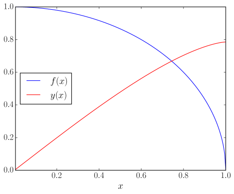
Figure 1: (Color online) Plots of the functions given in Eqs. (14) and (15). $f$ varies very rapidly towards the upper integration limit causing numerical difficulty.

The calculated value of the integral is $y(1)=0.785398163397448$ which has a $\delta_{\rm{rel}}$ of $\approx 1.414\times 10^{-16}$ compared to the exact value. It took $N=974$ function evaluations and $i_{\rm{max}}=35$ steps to propagate the integral $y$ from $0$ to $1$, where the size of the first step was set to $0.5$ as mentioned above. As can be seen from Fig. (2), the step sizes chosen by our algorithm kept decreasing to as low as $2.22\times 10^{-11}$, which is consistent with the singularity of the derivative of the integrand $f$ at the upper integration limit.

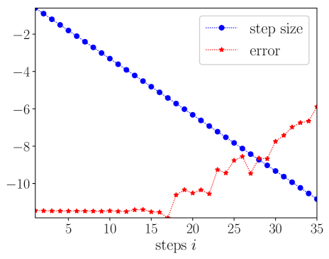
Figure 2: (Color online) Step size of the finite elements (blue .) and $\delta_{\rm{rel}}$ of the integral at the end of the elements (red *) are shown. The algorithm spends more time and picks up more errors towards the upper integration limit. Vertical axis values are $\log{}_{10}$ of the actual.

Fig. (2) also shows relative errors of the integral $y$ at the end of all the elements in comparison with the exact values from eq. (15).

Clearly, the maximum error occurs at the last step near $1$, which is what motivated our choice of this example. Rapidly changing functions, such as those with integrable singularity, are generally troublesome to the algorithm because the step size may not be small enough and/or the order of polynomials high enough to accommodate portions of the integrand with (nearly) vertical shape.

In comparison, DQAG takes $795$ function evaluations and calculates the integral with a $\delta_{\rm{rel}}$ of $2.827\times 10^{-16}$.

3.2 Nonlinear Problem

Bender et al. have studied the following interesting nonlinear eigenvalue problem for which the numerical solution can be very challenging [9].

$$\frac{{\rm{d}}}{{\rm{d}}x}y(x)=\cos\left[\pi xy(x)\right],\qquad x\geq 0$$ (16)

Since this is a nonlinear equation, it has to be solved in an iterative fashion as:

$$\frac{{\rm{d}}}{{\rm{d}}x}y_{\sigma+1}(x)=f_{\sigma}(x),\qquad\sigma=1,2,\ldots$$ (17)

where $f_{\sigma}(x)=\cos\left[\pi xy_{\sigma}(x)\right]$ and $\sigma$ labels the levels of the iteration. Notice that at any stage of the iteration only the values of $f$ at the GL nodes are required. The first iterate of array $f_{1}$ is seeded from the solution vector $B$ of the final result in the preceding element. This is not only convenient but also an excellent approximation because the adaptive step choice implemented here is based on the assumption that the solution function between two consecutive elements remains constant up to a fourth order Taylor series expansion. The first element has been started by setting all the elements of the solution vector $B$ to unity. Apparently, only for this problem, the first two steps of the procedure given in Section 2, must be repeated until the iteration in eq. (17) converges.

The results of our calculation for $y(x),x\in[0,24]$, are plotted in fig. 3 for initial values at the origin $y_{a}=n,n=1,2,\ldots,10$.

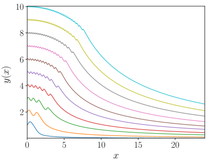
Figure 3: (Color online) Calculated solution functions to eq. (16) for $0\leq x\leq 24$ with initial condition $y_{a}=1,2,\ldots,10$ are shown. The functions are oscillatory near the origin before they evolve into an asymptotic discrete bundle.

Similar plots have been reported in ref. [9] which are a result of point–wise convergent calculations. Our solution function, on the other hand, has been propagated from the origin outward. The very large number of steps the solution required for such a modest distance of $x=24$ is quite remarkable. Table 1 summarizes the output of our program.

Table 2: Results for $y(24)$ to eq. (16) for the respective initial conditions $y(0)$. The rest of the columns are: total number of steps, average step size, average number of functions evaluations per element and time elapsed.

$y(0)$	$y(24)$	$i_{\rm{max}}$	$2q_{\rm{ave}}\,(\times 10^{-5})$	$N_{\rm{ave}}$	$t\,[sec]$
$1$	0.020 844 865 419 015 3	1 633 376	1.469	254.338	63
$2$	0.104 224 327 270 128	1 701 378	1.411	253.336	66
$3$	0.270 983 253 633 302	1 908 989	1.257	251.829	73
$4$	0.437 742 187 280 245	2 068 413	1.160	250.609	79
$5$	0.687 880 611 222 152	2 397 070	1.001	249.380	91
$6$	0.938 019 076 811 230	2 636 633	0.9103	248.157	100
$7$	1.271 537 122 002 93	3 041 709	0.7890	247.071	116
$8$	1.688 434 875 810 57	3 586 933	0.6691	245.951	135
$9$	2.105 332 915 403 23	4 021 621	0.5968	244.952	151
$10$	2.605 611 041 676 66	4 626 563	0.5187	244.110	174

It took millions of steps, with an average step size as low as $\approx 5.187\times 10^{-6}$ and an average number of function evaluations up to $N_{\rm{ave}}\approx 254.3$ per element. Notice that this $N_{\rm{ave}}$ includes all the iterations, which, along with the brevity of the elapsed times shown, indicates the efficiency of our implementation.

We have also included the final numerical values at $y(24)$ for reference. For this example, the required error has been set lower as $\delta_{\rm{rel}}=3.0\times 10^{-9}$, for an obvious reason. In order to check the validity our results, we have re–run the program by still lowering the magnitude of the error to $\delta_{\rm{rel}}=3.0\times 10^{-10}$. With the lowered error, the indicated values of $y(24)$ vary by an amount no larger than $\sim 1.86\times 10^{-13}$. The computational times in the last column of the table also increased to as high as $470$ seconds. Maintaining this much accuracy after millions of steps, and in an iterative calculation, shows how robust our method is. This non–linear eigenvalue problem is computationally challenging indeed.

3.3 Double–Range Integrals

In this example, we consider a double integral for which one of the limits of the inner integral is identical to the variable of the outer integral. These types of integrals are common in studies of many particle dynamical systems involving Green’s functions or double range addition theorems such as the Laplace expansion. Particularly, we will look at the following integral, which is the most prominent radial integral that is encountered in calculations that involve exponential type orbitals or Geminals in a spherical coordinate system. It stems from the addition theorem for ${r_{12}}^{n}e^{-\alpha r_{12}}$ given in [10] and the resulting integrals are still topics of interest in recent research [11, 12, 13]. Let us define the integral as

$$I_{\lambda_{1}\lambda_{2}}^{\mu_{1}\mu_{2}}(\alpha_{1},\beta_{1},\alpha_{2},\beta_{2})=\int_{0}^{\infty}{\rm{d}}y\,e^{-\alpha_{1}y}y^{{\mu}_{1}}\hat{i}_{\lambda_{1}}(\beta_{1}y)\int_{y}^{\infty}{\rm{d}}x\,e^{-\alpha_{2}x}x^{{\mu}_{2}}\hat{k}_{\lambda_{2}}(\beta_{2}x)$$ (18)

where $\hat{i}$ and $\hat{k}$ are spherical modified Bessel functions of the first and second kind respectively [4]. The screening parameters $\alpha_{1},\beta_{1},\alpha_{2},\beta_{2}$ are positive real numbers while all of the indices $\mu_{1},\lambda_{1},\mu_{2},\lambda_{2}$ are integers. The correct composition of these parameters is such that both the inner and outer integrals remain finite as is the case in physical applications.

In order to propagate from the origin, both lower integration limits need to be set to zero. This can be attained by switching the order of the two integrals using the following identity which maintains identical $x$–$y$ region of integration [14].

$$\int_{0}^{\infty}{\rm{d}}y\,f(y)\int_{y}^{\infty}{\rm{d}}x\,g(x)\equiv\int_{0}^{\infty}{\rm{d}}x\,g(x)\int_{0}^{x}{\rm{d}}y\,f(y)$$ (19)

Hence, eq. (18) can be written as

$$I_{\lambda_{1}\lambda_{2}}^{\mu_{1}\mu_{2}}(\alpha_{1},\beta_{1},\alpha_{2},\beta_{2})=\int_{0}^{\infty}{\rm{d}}x\,e^{-\alpha_{2}x}x^{{\mu}_{2}}\hat{k}_{\lambda_{2}}(\beta_{2}x)J_{\lambda_{1}}^{\mu_{1}}(\alpha_{1},\beta_{1};x)$$ (20)

where, $J$ now represents the inner integral given below which needs to be propagated only once from the origin until the integral converges.

$$J_{\lambda_{1}}^{\mu_{1}}(\alpha_{1},\beta_{1};x)=\int_{0}^{x}{\rm{d}}y\,e^{-\alpha_{1}y}y^{{\mu}_{1}}\hat{i}_{\lambda_{1}}(\beta_{1}y),\qquad 0\leq x\leq x_{i_{\rm{max}}+1}$$ (21)

Here $x_{i_{\rm{max}}+1}$ signifies the end point of the last element where the result of the above integral converged to its value at infinity. Hence, beyond this point $J$ is considered to be constant function, i.e., $J(x)=J(x_{i_{\rm{max}}+1})$ for $x>x_{i_{\rm{max}}+1}$. Once the above integral is done and all the relevant parameters stored, it can be evaluated at any desired point $x>0$, which is a significant computational gain since the double integral $I$ given in eq. (18) has essentially been reduced to two simple integrals. This demonstrates one of the main advantages contained in the present algorithm.

Table 3 shows a sample calculation for the integral $I$ in eq. (20) for $\beta_{1},\beta_{2}\in\{0.5,1.0,2.0\}$.

Table 3: Exact and calculated values of the integral $I$ are shown for $\beta_{1}$ & $\beta_{2}\in\{0.5,1.0,2.0\}$. Columns 3 and 4 show the number of function evaluations $N$ taken in the integrals Eq. (20) and Eq. (19) respectively. Numbers in square bracket signify powers of ten.

$\beta_{1}$	$\beta_{2}$	N of $J$	N of $I$	I – calculated	I – exact
$0.5$	0.5	219	259	1.627 473 168 386 65 [27]	1.627 473 168 386 653 87 [27]
$0.5$	1.0	219	218	2.559 085 779 949 79 [22]	2.559 085 779 949 794 01 [22]
$0.5$	2.0	219	231	3.103 777 873 917 21 [17]	3.103 777 873 917 210 86 [17]
$1.0$	0.5	232	259	2.946 389 365 576 82 [23]	2.946 389 365 576 741 23 [23]
$1.0$	1.0	232	245	6.062 810 005 197 87 [18]	6.062 810 005 197 874 73 [18]
$1.0$	2.0	232	204	9.533 337 428 978 80 [13]	9.533 337 428 978 808 27 [13]
$2.0$	0.5	245	259	4.342 544 722 241 59 [19]	4.342 544 722 241 718 83 [19]
$2.0$	1.0	245	245	1.097 615 571 907 40 [15]	1.097 615 571 907 438 80 [15]
$2.0$	2.0	245	231	2.258 572 729 378 12 [10]	2.258 572 729 378 146 95 [10]

The rest of the parameters are set as $\lambda_{1}=-11,\mu_{1}=12,\lambda_{2}=-13,\mu_{2}=14,\alpha_{1}=2\beta_{1},\alpha_{2}=2\beta_{2}$. The Bessel functions $\hat{i}$ and $\hat{k}$ have been computed using the subroutines in GNU Scientific Library (GSL) . For the first element, eq. (12) has been used in order to avoid evaluation at the origin. We also have calculated the exact values of the integrals using Mathematica [15], the first 18 digits of which are displayed in the last column. Comparison with the the present calculated results reveals that the integral $I$ was done accurately. The table also further shows the total number of function evaluations $N$ for the inner and outer integrals.

4 Conclusion

There are many physical applications that can be modeled as initial value problems and the methods available to compute them are equally diverse. No single algorithm is known to address all of them at once, and hence, researchers usually digress from their main area of interest so as to familiarize themselves with many of the computational options. The present algorithm is by no means capable of solving all initial value problems, but it comes pragmatically close, especially for most physical applications. This is possible because it produces solutions on finite elements whose size is chosen to locally, checks the validity of the solution, and communicates the solution function and its first derivative to the next element, maintaining continiuity of both. More importantly, it can be applied on any ODE because it is easy to implement and modify, especially with the proper use of object–oriented programming techniques. The basis functions $u$ and $s$ discussed above are based on Legendre polynomials. In the future, we will use other classic orthogonal polynomials such as Chebyshev or Jacobi to determine if further advantages can be gained.

5 Acknowledgement

DHG and CAW were partially supported by the Department of Energy, National Nuclear Security Administration, under Award Number(s) DE-NA0002630. CAW was also supported in part by the Defense Threat Reduction Agency.

6 REFERENCES

References

-
[1]
P. Davis, P. Rabinowitz,
Methods of Numerical
Integration, Dover Books on Mathematics Series, Dover Publications, 2007.
URL https://books.google.com/books?id=gGCKdqka0HAC -
[2]
D. H. Gebremedhin, C. A. Weatherford,
Calculations for
the one-dimensional soft coulomb problem and the hard coulomb limit, Phys.
Rev. E 89 (2014) 053319.
doi:10.1103/PhysRevE.89.053319.
URL http://link.aps.org/doi/10.1103/PhysRevE.89.053319 -
[3]
P. Kythe, P. Puri,
Computational Methods
for Linear Integral Equations, Birkhäuser Boston, 2002.
URL https://books.google.com/books?id=CmX1aHur7jcC - [4] G. B. Arfken, H. J. Weber, F. E. Harris, Mathematical Methods for Physicists, Sixth Edition: A Comprehensive Guide, 6th Edition, Academic Press, 2005.
- [5] W. H. Press, S. A. Teukolsky, W. T. Vetterling, B. P. Flannery, Numerical Recipes in FORTRAN (2Nd Ed.): The Art of Scientific Computing, Cambridge University Press, New York, NY, USA, 1992.
-
[6]
S. Ehrich, Applications
and Computation of Orthogonal Polynomials: Conference at the Mathematical
Research Institute Oberwolfach, Germany March 22–28, 1998, Birkhäuser
Basel, Basel, 1999, Ch. Stieltjes Polynomials and the Error of Gauss-Kronrod
Quadrature Formulas, pp. 57–77.
doi:10.1007/978-3-0348-8685-7\_4.
URL http://dx.doi.org/10.1007/978-3-0348-8685-7_4 -
[7]
R. Piessens, E. d. Doncker-Kapenga, C. Überhuber, D. Kahaner,
Quadpack, Springer
Series in Computational Mathematics, Springer-Verlag Berlin Heidelberg, 1983.
URL http://www.springer.com/us/book/9783540125532 -
[8]
D. H. Bailey, K. Jeyabalan, X. S. Li,
A comparison of three
high-precision quadrature schemes, Experimental Mathematics 14 (3) (2005)
317–329.
arXiv:http://dx.doi.org/10.1080/10586458.2005.10128931, doi:10.1080/10586458.2005.10128931.
URL http://dx.doi.org/10.1080/10586458.2005.10128931 -
[9]
C. M. Bender, A. Fring, J. Komijani,
Nonlinear eigenvalue
problems, Journal of Physics A: Mathematical and Theoretical 47 (23) (2014)
235204.
URL http://stacks.iop.org/1751-8121/47/i=23/a=235204 -
[10]
D. Gebremedhin, C. Weatherford,
Canonical two-range addition
theorem for slater-type orbitals, International Journal of Quantum Chemistry
113 (1) (2013) 71–75.
doi:10.1002/qua.24319.
URL http://dx.doi.org/10.1002/qua.24319 -
[11]
L. G. Jiao, Y. K. Ho,
Computation
of two-electron screened coulomb potential integrals in hylleraas basis
sets, Computer Physics Communications 188 (2015) 140 – 147.
doi:http://dx.doi.org/10.1016/j.cpc.2014.11.019.
URL http://www.sciencedirect.com/science/article/pii/S0010465514004020 -
[12]
J. F. Rico, R. López, G. Ramírez, I. Ema,
Repulsion integrals
involving slater-type functions and yukawa potential, Theoretical Chemistry
Accounts 132 (1) (2012) 1–9.
doi:10.1007/s00214-012-1304-x.
URL http://dx.doi.org/10.1007/s00214-012-1304-x -
[13]
J. J. Fern ndez, R. L pez, I. Ema, G. Ram rez, J. Fern ndez Rico,
Auxiliary functions for molecular
integrals with slater-type orbitals. i. translation methods, International
Journal of Quantum Chemistry 106 (9) (2006) 1986–1997.
doi:10.1002/qua.21002.
URL http://dx.doi.org/10.1002/qua.21002 - [14] S. Hassani, Mathematical Methods: For Students of Physics and Related Fields, Undergraduate Texts in Contemporary Physics, Springer New York, 2000.
- [15] Mathematica, Version 7.0 1.0, Wolfram Research, Champaign, Illinois, 2009.