Nonlinear coupling of photons via a collective mode of transparent superconductor
V. M. Akulin
Laboratoire Aimé Cotton, CNRS (UPR 3321), Bâtiment 505, 91405 Orsay
Cedex, France.
Institute for Information Transmission Problems of the Russian Academy of
Science, Bolshoy Karetny per. 19, Moscow, 127994, Russia.
Laboratoire J.-V. Poncelet CNRS (UMI 2615) Bolshoi Vlassievsky per. 11,
Moscow, 119002 Russia.
Abstract
At the first glance, the expression ”transparent superconductor” may seem an
oxymoron. Still, the first principle calculationsNakanishi Exp e 2 / m superscript 𝑒 2 𝑚 e^{2}/m μ 𝜇 \mu c m 𝑐 𝑚 cm
pacs: 03.65.-w Quantum mechanics, 42.65.Wi Nonlinear waveguides, 78.20.Bh Theory,
models, and numerical simulation.
† † preprint: ω k ′ ω k subscript 𝜔 superscript 𝑘 ′ subscript 𝜔 𝑘 \omega_{k^{\prime}}\omega_{k}
Interaction of photons mediated by atomic or condensed-matter electrons gets
stronger when the latter are in a collective or a cooperativeDicke Abrikosov Kulik Klein Nakanishi p 𝑝 p C u A l O 2 𝐶 𝑢 𝐴 𝑙 subscript 𝑂 2 CuAlO_{2}
The non-relativistic Pauli equation for an electron in an external quantized
electromagnetic field suggests the interaction term in the form− e m c p → ^ A → ^ + e 2 A → ^ 2 2 m c 2 𝑒 𝑚 𝑐 ^ → 𝑝 ^ → 𝐴 superscript 𝑒 2 superscript ^ → 𝐴 2 2 𝑚 superscript 𝑐 2 -\frac{e}{mc}\widehat{\overrightarrow{p}}\widehat{\overrightarrow{A}}+\frac{e^{2}\widehat{\overrightarrow{A}}^{2}}{2mc^{2}}
A → ^ ( r → ) = ∑ k c π ℏ v ω k ( a ^ k u → k ( r → ) + a ^ k + u → k ∗ ( r → ) ) ^ → 𝐴 → 𝑟 subscript 𝑘 𝑐 𝜋 Planck-constant-over-2-pi 𝑣 subscript 𝜔 𝑘 subscript ^ 𝑎 𝑘 subscript → 𝑢 𝑘 → 𝑟 superscript subscript ^ 𝑎 𝑘 superscript subscript → 𝑢 𝑘 ∗ → 𝑟 \widehat{\overrightarrow{A}}(\overrightarrow{r})=\sum_{k}\sqrt{\frac{c\pi\hbar v}{\omega_{k}}}\left(\widehat{a}_{k}\overrightarrow{u}_{k}\left(\overrightarrow{r}\right)+\widehat{a}_{k}^{+}\overrightarrow{u}_{k}^{\ast}\left(\overrightarrow{r}\right)\right) (1)
is given in terms of photon frequency ω k subscript 𝜔 𝑘 \omega_{k} v 𝑣 v UFN a ^ k + superscript subscript ^ 𝑎 𝑘 \widehat{a}_{k}^{+} a ^ k subscript ^ 𝑎 𝑘 \widehat{a}_{k} u → k ( r → ) subscript → 𝑢 𝑘 → 𝑟 \overrightarrow{u}_{k}\left(\overrightarrow{r}\right) ∫ u → k u → k ∗ 𝑑 V = 1 subscript → 𝑢 𝑘 superscript subscript → 𝑢 𝑘 ∗ differential-d 𝑉 1 \int\overrightarrow{u}_{k}\overrightarrow{u}_{k}^{\ast}dV=1
From the viewpoint of the relativistic Dirac equation, the pondermotor term
e 2 A → ^ 2 / 2 m c 2 superscript 𝑒 2 superscript ^ → 𝐴 2 2 𝑚 superscript 𝑐 2 e^{2}\widehat{\overrightarrow{A}}^{2}/2mc^{2} MichaFedorov − e m c p → ^ A → ^ 𝑒 𝑚 𝑐 ^ → 𝑝 ^ → 𝐴 -\frac{e}{mc}\widehat{\overrightarrow{p}}\widehat{\overrightarrow{A}} e 2 A → ^ 2 / 2 m c 2 superscript 𝑒 2 superscript ^ → 𝐴 2 2 𝑚 superscript 𝑐 2 e^{2}\widehat{\overrightarrow{A}}^{2}/2mc^{2} ∼ similar-to \sim v F / c subscript 𝑣 𝐹 𝑐 v_{F}/c I
For a multi-electron system with the electron density n e subscript 𝑛 𝑒 n_{e} n e e 2 A → 2 / 2 m c 2 ≡ ( ω p / ω k ) 2 E → 2 / 8 π subscript 𝑛 𝑒 superscript 𝑒 2 superscript → 𝐴 2 2 𝑚 superscript 𝑐 2 superscript subscript 𝜔 𝑝 subscript 𝜔 𝑘 2 superscript → 𝐸 2 8 𝜋 n_{e}e^{2}\overrightarrow{A}^{2}/2mc^{2}\equiv\left(\omega_{p}/\omega_{k}\right)^{2}\overrightarrow{E}^{2}/8\pi ω p = 4 π n e e 2 / m subscript 𝜔 𝑝 4 𝜋 subscript 𝑛 𝑒 superscript 𝑒 2 𝑚 \omega_{p}=\sqrt{4\pi n_{e}e^{2}/m} ω k < ω p subscript 𝜔 𝑘 subscript 𝜔 𝑝 \omega_{k}<\omega_{p} λ p ∼ 2 π ω k / c ( ω p / ω k ) 2 − 1 similar-to subscript 𝜆 𝑝 2 𝜋 subscript 𝜔 𝑘 𝑐 superscript subscript 𝜔 𝑝 subscript 𝜔 𝑘 2 1 \lambda_{p}\sim 2\pi\omega_{k}/c\sqrt{\left(\omega_{p}/\omega_{k}\right)^{2}-1} λ p subscript 𝜆 𝑝 \lambda_{p} ω k subscript 𝜔 𝑘 \omega_{k} ω k ′ subscript 𝜔 superscript 𝑘 ′ \omega_{k^{\prime}}
n ^ e e 2 π ℏ v 2 m c ∑ k ; k ′ a ^ k a ^ k ′ + u → k ′ ∗ ( r → ) u → k ( r → ) + h . c . ω k ′ ω k , \widehat{n}_{e}\frac{e^{2}\pi\hbar v}{2mc}\sum_{k;k^{\prime}}\frac{\widehat{a}_{k}\widehat{a}_{k^{\prime}}^{+}\overrightarrow{u}_{k^{\prime}}^{\ast}\left(\overrightarrow{r}\right)\overrightarrow{u}_{k}\left(\overrightarrow{r}\right)+h.c.}{\sqrt{\omega_{k^{\prime}}\omega_{k}}}, (2)
one can retain only the terms oscillating at the photon frequency difference,
which can be tuned close to the resonance with collective modes of the
superconductor. Here n ^ e = ψ ^ † ( r → ) ψ ^ ( r → ) subscript ^ 𝑛 𝑒 superscript ^ 𝜓 † → 𝑟 ^ 𝜓 → 𝑟 \widehat{n}_{e}=\widehat{\psi}^{{\dagger}}(\overrightarrow{r})\widehat{\psi}(\overrightarrow{r}) ψ ^ † ( r → ) superscript ^ 𝜓 † → 𝑟 \widehat{\psi}^{{\dagger}}(\overrightarrow{r}) ψ ^ ( r → ) ^ 𝜓 → 𝑟 \widehat{\psi}(\overrightarrow{r}) h . c . formulae-sequence ℎ 𝑐 h.c.
Consider now such a system for the case of a superconductor at zero
temperature in a static sub-critical magnetic field given by the vector
potential A → s t subscript → 𝐴 𝑠 𝑡 \overrightarrow{A}_{st} ω k ≅ ω subscript 𝜔 𝑘 𝜔 \omega_{k}\cong\omega ω k ′ ≅ ω + δ ω subscript 𝜔 superscript 𝑘 ′ 𝜔 𝛿 𝜔 \omega_{k^{\prime}}\cong\omega+\delta\omega ℏ δ ω Planck-constant-over-2-pi 𝛿 𝜔 \hbar\delta\omega Δ ( r → ) Δ → 𝑟 \Delta(\overrightarrow{r}) m = 1 𝑚 1 m=1 ℏ = 1 Planck-constant-over-2-pi 1 \hbar=1 e = 1 𝑒 1 e=1 − g 𝑔 -g
H ^ ^ 𝐻 \displaystyle\widehat{H} = ∫ d V [ 1 2 ψ ^ s † ( r → ) ( p → ^ − A → ^ s t / c ) 2 ψ ^ s ( r → ) \displaystyle=\int dV\left[\frac{1}{2}\widehat{\psi}_{s}^{{\dagger}}(\overrightarrow{r})\left(\widehat{\overrightarrow{p}}-\widehat{\overrightarrow{A}}_{st}/c\right)^{2}\widehat{\psi}_{s}(\overrightarrow{r})\right. (3)
− 1 2 Δ ^ ( r → ) ψ ^ s † ( r → ) ψ ^ − s † ( r → ) − 1 2 Δ ^ † ( r → ) ψ ^ s ( r → ) ψ ^ − s ( r → ) 1 2 ^ Δ → 𝑟 superscript subscript ^ 𝜓 𝑠 † → 𝑟 superscript subscript ^ 𝜓 𝑠 † → 𝑟 1 2 superscript ^ Δ † → 𝑟 subscript ^ 𝜓 𝑠 → 𝑟 subscript ^ 𝜓 𝑠 → 𝑟 \displaystyle-\frac{1}{2}\widehat{\Delta}(\overrightarrow{r})\widehat{\psi}_{s}^{{\dagger}}(\overrightarrow{r})\widehat{\psi}_{-s}^{{\dagger}}(\overrightarrow{r})-\frac{1}{2}\widehat{\Delta}^{{\dagger}}(\overrightarrow{r})\widehat{\psi}_{s}(\overrightarrow{r})\widehat{\psi}_{-s}(\overrightarrow{r})
+ 1 2 g Δ ^ † ( r → ) Δ ^ ( r → ) + π v 2 c ψ ^ s † ( r → ) ψ ^ s ( r → ) × ∑ k ; k ′ 1 2 𝑔 superscript ^ Δ † → 𝑟 ^ Δ → 𝑟 𝜋 𝑣 2 𝑐 superscript subscript ^ 𝜓 𝑠 † → 𝑟 subscript ^ 𝜓 𝑠 → 𝑟 subscript 𝑘 superscript 𝑘 ′
\displaystyle+\frac{1}{2g}\widehat{\Delta}^{{\dagger}}(\overrightarrow{r})\widehat{\Delta}(\overrightarrow{r})+\frac{\pi v}{2c}\widehat{\psi}_{s}^{{\dagger}}(\overrightarrow{r})\widehat{\psi}_{s}(\overrightarrow{r})\times\sum_{k;k^{\prime}}
a ^ k a ^ k ′ + u → k ′ ∗ ( r → ) u → k ( r → ) + h . c . ω k ′ ω k ] + ∑ k ω k ( a ^ k + a ^ k + 1 2 ) \displaystyle\left.\frac{\widehat{a}_{k}\widehat{a}_{k^{\prime}}^{+}\overrightarrow{u}_{k^{\prime}}^{\ast}\left(\overrightarrow{r}\right)\overrightarrow{u}_{k}\left(\overrightarrow{r}\right)+h.c.}{\sqrt{\omega_{k^{\prime}}\omega_{k}}}\right]+\sum_{k}\omega_{k}\left(\widehat{a}_{k}^{+}\widehat{a}_{k}+\frac{1}{2}\right)
where summation over the spin subscripts s = ± 𝑠 plus-or-minus s=\pm ± 1 / 2 plus-or-minus 1 2 \pm 1/2
In the case where photons are out of resonance with the superconductor
excitations, the interaction among them can be considered as the second order
perturbation, such that the photon part of the Hamiltonian adopts the form
H ^ = ∑ k ω k ( a ^ k + a ^ k + 1 2 ) + ∑ k k ′ χ k , k ′ , k ′ , k ( δ ω ) a ^ k a ^ k ′ + a ^ k ′ a ^ k + , ^ 𝐻 subscript 𝑘 subscript 𝜔 𝑘 superscript subscript ^ 𝑎 𝑘 subscript ^ 𝑎 𝑘 1 2 subscript 𝑘 superscript 𝑘 ′ subscript 𝜒 𝑘 superscript 𝑘 ′ superscript 𝑘 ′ 𝑘
𝛿 𝜔 subscript ^ 𝑎 𝑘 superscript subscript ^ 𝑎 superscript 𝑘 ′ subscript ^ 𝑎 superscript 𝑘 ′ superscript subscript ^ 𝑎 𝑘 \widehat{H}=\sum_{k}\omega_{k}\left(\widehat{a}_{k}^{+}\widehat{a}_{k}+\frac{1}{2}\right)+\sum_{kk^{\prime}}\chi_{k,k^{\prime},k^{\prime},k}\left(\delta\omega\right)\widehat{a}_{k}\widehat{a}_{k^{\prime}}^{+}\widehat{a}_{k^{\prime}}\widehat{a}_{k}^{+}, (4)
which implies that the nonlinear coupling of photons occur via the linear
susceptibility of the multielectronic system to the pondermotor perturbation
A → ^ 2 / 2 c 2 superscript ^ → 𝐴 2 2 superscript 𝑐 2 \widehat{\overrightarrow{A}}^{2}/2c^{2} χ k , k ′ , k ′ , k subscript 𝜒 𝑘 superscript 𝑘 ′ superscript 𝑘 ′ 𝑘
\chi_{k,k^{\prime},k^{\prime},k}
It is convenient to invoke a standard technique – the Feynmann integration
over the anticommuting electron fields and classical fields for the order
parameterKleinert
χ k , k ′ , k ′ , k = ∂ 2 ∂ α ∂ α ∗ ln Z ( α ∗ , α ) , subscript 𝜒 𝑘 superscript 𝑘 ′ superscript 𝑘 ′ 𝑘
superscript 2 𝛼 superscript 𝛼 ∗ 𝑍 superscript 𝛼 ∗ 𝛼 \chi_{k,k^{\prime},k^{\prime},k}=\frac{\partial^{2}}{\partial\alpha\partial\alpha^{\ast}}\ln Z\left(\alpha^{\ast},\alpha\right), (5)
where the ”partition function” Z 𝑍 Z
Z = ∫ e i S D ψ + ∗ D ψ + D ψ − ∗ D ψ − D Δ 1 ∗ D Δ 1 D Δ 2 ∗ D Δ 2 𝑍 superscript 𝑒 𝑖 𝑆 𝐷 superscript subscript 𝜓 ∗ 𝐷 subscript 𝜓 𝐷 superscript subscript 𝜓 ∗ 𝐷 subscript 𝜓 𝐷 superscript subscript Δ 1 ∗ 𝐷 subscript Δ 1 𝐷 superscript subscript Δ 2 ∗ 𝐷 subscript Δ 2 Z=\int e^{iS}D\psi_{+}^{\ast}D\psi_{+}D\psi_{-}^{\ast}D\psi_{-}D\Delta_{1}^{\ast}D\Delta_{1}D\Delta_{2}^{\ast}D\Delta_{2} (6)
with the action
S 𝑆 \displaystyle S = ∫ ( ψ + ∗ ψ + ∗ ψ − ψ − ) M ^ ( ψ + ψ + ψ − ∗ ψ − ∗ ) d ω ~ 2 d 3 k ~ absent superscript subscript 𝜓 ∗ superscript subscript 𝜓 ∗ subscript 𝜓 subscript 𝜓 ^ 𝑀 subscript 𝜓 subscript 𝜓 superscript subscript 𝜓 ∗ superscript subscript 𝜓 ∗ 𝑑 ~ 𝜔 2 superscript 𝑑 3 ~ 𝑘 \displaystyle=\int\left(\begin{array}[c]{cccc}\psi_{+}^{\ast}&\psi_{+}^{\ast}&\psi_{-}&\psi_{-}\end{array}\right)\widehat{M}\left(\begin{array}[c]{c}\psi_{+}\\
\psi_{+}\\
\psi_{-}^{\ast}\\
\psi_{-}^{\ast}\end{array}\right)\frac{d\widetilde{\omega}}{2}d^{3}\widetilde{k} (12)
+ ∫ 1 2 g δ Δ ∗ ( ω , k → ) δ Δ ( ω , k ~ → ) 𝑑 ω ~ d 3 k ~ . 1 2 𝑔 𝛿 superscript Δ ∗ 𝜔 → 𝑘 𝛿 Δ 𝜔 → ~ 𝑘 differential-d ~ 𝜔 superscript 𝑑 3 ~ 𝑘 \displaystyle+\int\frac{1}{2g}\delta\Delta^{\ast}(\omega,\overrightarrow{k})\delta\Delta(\omega,\overrightarrow{\widetilde{k}})d\widetilde{\omega}d^{3}\widetilde{k}. (13)
The Hamiltonian Eq.(3 M ^ ^ 𝑀 \widehat{M} Expr
( δ ω + ω ~ − ϵ 1 α ∗ u → k ∗ u → k ′ − Δ 1 − Δ α u → k ′ ∗ u → k ω ~ − ϵ 2 − Δ − Δ 2 − Δ ∗ 1 − Δ ∗ ω ~ + ϵ 3 − α u → k ′ ∗ u → k − Δ ∗ − Δ 2 ∗ − α ∗ u → k ∗ u → k ′ δ ω + ω ~ + ϵ 4 ) . \left(\begin{array}[c]{cccc}\delta\omega+\widetilde{\omega}-\text{$\epsilon_{1}$}&\alpha^{\ast}\overrightarrow{u}_{k}^{\ast}\overrightarrow{u}_{k^{\prime}}&-\Delta\text{${}_{1}$}&-\Delta\\
\alpha\overrightarrow{u}_{k^{\prime}}^{\ast}\overrightarrow{u}_{k}&\widetilde{\omega}-\text{$\epsilon_{2}$}&-\Delta&-\Delta_{2}\\
-\Delta^{\ast}\text{${}_{1}$}&-\text{$\Delta^{\ast}$}&\widetilde{\omega}+\text{$\epsilon_{3}$}&-\alpha\overrightarrow{u}_{k^{\prime}}^{\ast}\overrightarrow{u}_{k}\\
-\text{$\Delta^{\ast}$}&-\Delta_{2}^{\ast}&-\alpha^{\ast}\overrightarrow{u}_{k}^{\ast}\overrightarrow{u}_{k^{\prime}}&\delta\omega+\widetilde{\omega}+\text{$\epsilon_{4}$}\end{array}\right). (14)
Here α 𝛼 \alpha α ∗ superscript 𝛼 ∗ \alpha^{\ast} a ^ k a ^ k ′ + subscript ^ 𝑎 𝑘 superscript subscript ^ 𝑎 superscript 𝑘 ′ \widehat{a}_{k}\widehat{a}_{k^{\prime}}^{+} a ^ k ′ a ^ k + subscript ^ 𝑎 superscript 𝑘 ′ superscript subscript ^ 𝑎 𝑘 \widehat{a}_{k^{\prime}}\widehat{a}_{k}^{+} ϵ 2 , ϵ 3 subscript italic-ϵ 2 subscript italic-ϵ 3
\epsilon_{2},\epsilon_{3} ϵ 1 , ϵ 4 subscript italic-ϵ 1 subscript italic-ϵ 4
\epsilon_{1},\epsilon_{4} π v 2 c ω k 𝜋 𝑣 2 𝑐 subscript 𝜔 𝑘 \ \sqrt{\frac{\pi v}{2c\omega_{k}}} u → k subscript → 𝑢 𝑘 \overrightarrow{u}_{k} Δ 1 subscript Δ 1 \Delta_{1} Δ 2 subscript Δ 2 \Delta_{2} Δ Δ \Delta II
It is expedient to discuss the gap parameters of Eq.(14 Δ ( r → ) Δ → 𝑟 \Delta(\overrightarrow{r}) δ Δ = Δ 1 ( r → ) + Δ 2 ( r → ) 𝛿 Δ subscript Δ 1 → 𝑟 subscript Δ 2 → 𝑟 \delta\Delta=\Delta_{1}(\overrightarrow{r})+\Delta_{2}(\overrightarrow{r}) Leggett 2 | Δ | 2 Δ 2\left|\Delta\right| χ k , k ′ , k ′ , k subscript 𝜒 𝑘 superscript 𝑘 ′ superscript 𝑘 ′ 𝑘
\chi_{k,k^{\prime},k^{\prime},k} Δ 2 subscript Δ 2 \Delta_{2} Δ Δ \Delta Δ 1 subscript Δ 1 \Delta_{1} ∗
Figure 1: Degenerate tube modes L = ± 1 𝐿 plus-or-minus 1 L=\pm 1 n = 2.26 𝑛 2.26 n=2.26 R o u t / R i n n = 1.15 subscript 𝑅 𝑜 𝑢 𝑡 subscript 𝑅 𝑖 𝑛 𝑛 1.15 R_{out}/R_{inn}=1.15 u θ subscript 𝑢 𝜃 u_{\theta} u r subscript 𝑢 𝑟 u_{r} u r subscript 𝑢 𝑟 u_{r} u z subscript 𝑢 𝑧 u_{z} R i n n ω c n 2 − 1 subscript 𝑅 𝑖 𝑛 𝑛 𝜔 𝑐 superscript 𝑛 2 1 R_{inn}\frac{\omega}{c}\sqrt{n^{2}-1} k c ω − 1 n − 1 𝑘 𝑐 𝜔 1 𝑛 1 \frac{\frac{kc}{\omega}-1}{n-1} ω 0 subscript 𝜔 0 \omega_{0} k 𝑘 k k ′ superscript 𝑘 ′ k^{\prime}
Consider this situation for a specific setting shown in Fig.1 R 𝑅 R d ≪ λ p much-less-than 𝑑 subscript 𝜆 𝑝 d\ll\lambda_{p} n 𝑛 n r , θ , z 𝑟 𝜃 𝑧
r,\theta,z θ → L → 𝜃 𝐿 \theta\rightarrow L z → k → 𝑧 𝑘 z\rightarrow k u → k ( r → ) subscript → 𝑢 𝑘 → 𝑟 \overrightarrow{u}_{k}\left(\overrightarrow{r}\right) u → k ′ ( r → ) subscript → 𝑢 superscript 𝑘 ′ → 𝑟 \overrightarrow{u}_{k^{\prime}}\left(\overrightarrow{r}\right)
π v 2 l c ω k u → k ( r , z , θ ) 𝜋 𝑣 2 𝑙 𝑐 subscript 𝜔 𝑘 subscript → 𝑢 𝑘 𝑟 𝑧 𝜃 \displaystyle\sqrt{\frac{\pi v}{2lc\omega_{k}}}\overrightarrow{u}_{k}\left(r,z,\theta\right) = ( u z ( r ) u r ( r ) u θ ( r ) ) e − i ω t + i k z + i L θ absent subscript 𝑢 𝑧 𝑟 subscript 𝑢 𝑟 𝑟 subscript 𝑢 𝜃 𝑟 superscript 𝑒 𝑖 𝜔 𝑡 𝑖 𝑘 𝑧 𝑖 𝐿 𝜃 \displaystyle=\left(\begin{array}[c]{c}u_{z}\left(r\right)\\
u_{r}\left(r\right)\\
u_{\theta}\left(r\right)\end{array}\right)e^{-i\omega t+ikz+iL\theta} (18)
(19)
π v 2 l c ω k ′ u → k ′ ( r , z , θ ) 𝜋 𝑣 2 𝑙 𝑐 subscript 𝜔 superscript 𝑘 ′ subscript → 𝑢 superscript 𝑘 ′ 𝑟 𝑧 𝜃 \displaystyle\sqrt{\frac{\pi v}{2lc\omega_{k^{\prime}}}}\overrightarrow{u}_{k^{\prime}}\left(r,z,\theta\right) = ( u z ′ ( r ) u r ′ ( r ) u θ ′ ( r ) ) e − i ω ′ t + i k ′ z + i L ′ θ absent superscript subscript 𝑢 𝑧 ′ 𝑟 superscript subscript 𝑢 𝑟 ′ 𝑟 superscript subscript 𝑢 𝜃 ′ 𝑟 superscript 𝑒 𝑖 superscript 𝜔 ′ 𝑡 𝑖 superscript 𝑘 ′ 𝑧 𝑖 superscript 𝐿 ′ 𝜃 \displaystyle=\left(\begin{array}[c]{c}u_{z}^{\prime}\left(r\right)\\
u_{r}^{\prime}\left(r\right)\\
u_{\theta}^{\prime}\left(r\right)\end{array}\right)e^{-i\omega^{\prime}t+ik^{\prime}z+iL^{\prime}\theta} (23)
that correspond to two modes chosen to have close group velocities v 𝑣 v v ′ superscript 𝑣 ′ v^{\prime} π v 2 c ω k 𝜋 𝑣 2 𝑐 subscript 𝜔 𝑘 \sqrt{\frac{\pi v}{2c\omega_{k}}} l 𝑙 l u z ( r ) = − b q Z L ( r q ) / 2 k subscript 𝑢 𝑧 𝑟 𝑏 𝑞 subscript 𝑍 𝐿 𝑟 𝑞 2 𝑘 u_{z}\left(r\right)=-bqZ_{L}\left(rq\right)/2k u θ ( r ) = b L Z L ( r q ) / r q − a Z L ′ ( r q ) subscript 𝑢 𝜃 𝑟 𝑏 𝐿 subscript 𝑍 𝐿 𝑟 𝑞 𝑟 𝑞 𝑎 superscript subscript 𝑍 𝐿 ′ 𝑟 𝑞 u_{\theta}\left(r\right)=bLZ_{L}\left(rq\right)/rq-aZ_{L}^{\prime}\left(rq\right) u r ( r ) = a i L Z L ( r q ) / r q − b i Z L ′ ( r q ) subscript 𝑢 𝑟 𝑟 𝑎 𝑖 𝐿 subscript 𝑍 𝐿 𝑟 𝑞 𝑟 𝑞 𝑏 𝑖 superscript subscript 𝑍 𝐿 ′ 𝑟 𝑞 u_{r}\left(r\right)=aiLZ_{L}\left(rq\right)/rq-biZ_{L}^{\prime}\left(rq\right) Z L = K L subscript 𝑍 𝐿 subscript 𝐾 𝐿 Z_{L}=K_{L} Z L = I L subscript 𝑍 𝐿 subscript 𝐼 𝐿 Z_{L}=I_{L} Z L = γ J L + ϰ Y L subscript 𝑍 𝐿 𝛾 subscript 𝐽 𝐿 italic-ϰ subscript 𝑌 𝐿 Z_{L}=\gamma J_{L}+\varkappa Y_{L} ∫ 2 π r | u | 2 𝑑 r = 1 2 𝜋 𝑟 superscript 𝑢 2 differential-d 𝑟 1 \int 2\pi r\left|u\right|^{2}dr=1 q 𝑞 q k 2 − ω k 2 c − 2 superscript 𝑘 2 superscript subscript 𝜔 𝑘 2 superscript 𝑐 2 \sqrt{k^{2}-\omega_{k}^{2}c^{-2}} n 2 ω k 2 c − 2 − k 2 superscript 𝑛 2 superscript subscript 𝜔 𝑘 2 superscript 𝑐 2 superscript 𝑘 2 \sqrt{n^{2}\omega_{k}^{2}c^{-2}-k^{2}} ω k ( k ) subscript 𝜔 𝑘 𝑘 \omega_{k}\left(k\right) ω k ′ ( k ′ ) subscript 𝜔 superscript 𝑘 ′ superscript 𝑘 ′ \omega_{k^{\prime}}\left(k^{\prime}\right) III
For the electron energies, the cylindrical symmetry implies
ϵ f ( L ~ , k ~ ) = p r 2 2 + k ~ 2 2 + ( L ~ − L ¯ ) 2 R 2 − μ , subscript italic-ϵ 𝑓 ~ 𝐿 ~ 𝑘 superscript subscript 𝑝 𝑟 2 2 superscript ~ 𝑘 2 2 superscript ~ 𝐿 ¯ 𝐿 2 superscript 𝑅 2 𝜇 \text{$\epsilon_{f}$}(\widetilde{L},\widetilde{k})=\frac{p_{r}^{2}}{2}+\frac{\widetilde{k}^{2}}{2}+\frac{\left(\widetilde{L}-\overline{L}\right)^{2}}{R^{2}}-\mu, (24)
where k ~ ~ 𝑘 \widetilde{k} L ~ ~ 𝐿 \widetilde{L} p r subscript 𝑝 𝑟 p_{r} μ 𝜇 \mu A → s t subscript → 𝐴 𝑠 𝑡 \overrightarrow{A}_{st} L ¯ ¯ 𝐿 \overline{L} L ¯ ¯ 𝐿 \overline{L}
If a magnetic field corresponding to L ¯ = Λ ¯ 𝐿 Λ \overline{L}=\Lambda Δ Δ \Delta e i 2 Λ θ superscript 𝑒 𝑖 2 Λ 𝜃 e^{i2\Lambda\theta} L ¯ ¯ 𝐿 \overline{L} L ¯ ¯ 𝐿 \overline{L} Δ ( r → ) Δ → 𝑟 \Delta(\overrightarrow{r})
Now one can explicitly find the energies
ϵ 1 subscript italic-ϵ 1 \epsilon_{1} = ϵ f ( L ~ + δ L , k ~ + δ k ) absent subscript italic-ϵ 𝑓 ~ 𝐿 𝛿 𝐿 ~ 𝑘 𝛿 𝑘 \displaystyle=\epsilon_{f}(\widetilde{L}+\delta\text{$L$},\widetilde{k}+\delta\text{$k$})
ϵ 2 subscript italic-ϵ 2 \epsilon_{2} = ϵ f ( L ~ , k ~ ) absent subscript italic-ϵ 𝑓 ~ 𝐿 ~ 𝑘 \displaystyle=\epsilon_{f}(\widetilde{L},\widetilde{k})
ϵ 3 subscript italic-ϵ 3 \epsilon_{3} = ϵ f ( 2 Λ − L ~ , − k ~ ) absent subscript italic-ϵ 𝑓 2 Λ ~ 𝐿 ~ 𝑘 \displaystyle=\epsilon_{f}(2\Lambda-\widetilde{L},-\widetilde{k})
ϵ 4 subscript italic-ϵ 4 \epsilon_{4} = ϵ f ( 2 Λ − L ~ − δ L , − k ~ − δ k ) , absent subscript italic-ϵ 𝑓 2 Λ ~ 𝐿 𝛿 𝐿 ~ 𝑘 𝛿 𝑘 \displaystyle=\epsilon_{f}(2\Lambda-\widetilde{L}-\delta\text{$L$},-\widetilde{k}-\delta\text{$k$}), (25)
entering Eq.(14
δ Δ = Δ 1 e i z δ k − i t δ ω + i θ ( δ L + 2 Λ ) + Δ 2 e − i z δ k + i t δ ω − i θ ( δ L − 2 Λ ) 2 π d R l , 𝛿 Δ subscript Δ 1 superscript 𝑒 𝑖 𝑧 𝛿 𝑘 𝑖 𝑡 𝛿 𝜔 𝑖 𝜃 𝛿 𝐿 2 Λ subscript Δ 2 superscript 𝑒 𝑖 𝑧 𝛿 𝑘 𝑖 𝑡 𝛿 𝜔 𝑖 𝜃 𝛿 𝐿 2 Λ 2 𝜋 𝑑 𝑅 𝑙 \delta\Delta=\frac{\Delta_{1}e^{iz\delta k-it\delta\omega+i\theta\left(\delta L+2\Lambda\right)}+\Delta_{2}e^{-iz\delta k+it\delta\omega-i\theta\left(\delta L-2\Lambda\right)}}{\sqrt{2\pi dRl}}, (26)
normalized to the layer volume. Here δ k = k − k ′ 𝛿 𝑘 𝑘 superscript 𝑘 ′ \delta k=k-k^{\prime} δ L = L − L ′ 𝛿 𝐿 𝐿 superscript 𝐿 ′ \delta L=L-L^{\prime} Δ 1 , 2 subscript Δ 1 2
\Delta_{1,2} 14
Further a bit cumbersome but completely straightforward calculations can be
sketched as follows. Integration over the anticommuting fields ψ 𝜓 \psi
Z = ∫ e ∫ d ω ~ 2 Tr [ log ( det M ^ ) ] + i Δ 1 ∗ Δ 1 + Δ 2 ∗ Δ 2 2 g 𝑑 Δ 1 … 𝑑 Δ 2 ∗ , 𝑍 superscript 𝑒 𝑑 ~ 𝜔 2 Tr delimited-[] ^ 𝑀 𝑖 superscript subscript Δ 1 ∗ subscript Δ 1 superscript subscript Δ 2 ∗ subscript Δ 2 2 𝑔 differential-d subscript Δ 1 … differential-d superscript subscript Δ 2 ∗ Z=\int e^{\int\frac{d\widetilde{\omega}}{2}\mathrm{Tr}\left[\log\left(\det\widehat{M}\right)\right]+i\frac{\Delta_{1}^{\ast}\Delta_{1}+\Delta_{2}^{\ast}\Delta_{2}}{2g}}d\Delta_{1}\ldots d\Delta_{2}^{\ast}, (27)
where the first term in the exponent at the right hand side serves as an
action for the variables Δ 1 subscript Δ 1 \Delta_{1} Δ 2 subscript Δ 2 \Delta_{2} M ^ ^ 𝑀 \widehat{M} 14 25 d ω ~ 𝑑 ~ 𝜔 d\widetilde{\omega}
∫ 𝑑 ω ~ Tr [ log ( det M ^ ) ] ≃ ( α Δ 1 Δ 2 ∗ ) ℳ ~ ^ ( α ∗ Δ 1 ∗ Δ 2 ) similar-to-or-equals differential-d ~ 𝜔 Tr delimited-[] ^ 𝑀 𝛼 subscript Δ 1 superscript subscript Δ 2 ∗ ^ ~ ℳ superscript 𝛼 ∗ superscript subscript Δ 1 ∗ subscript Δ 2 \int d\widetilde{\omega}\mathrm{Tr}\left[\log\left(\det\widehat{M}\right)\right]\simeq\left(\begin{array}[c]{ccc}\alpha&\Delta_{1}&\Delta_{2}^{\ast}\end{array}\right)\widehat{\widetilde{\mathcal{M}}}\left(\begin{array}[c]{c}\alpha^{\ast}\\
\Delta_{1}^{\ast}\\
\Delta_{2}\end{array}\right) (28)
with
ℳ ~ ^ = ( ℳ ~ α , α − ℳ ~ Δ , α ℳ ~ Δ , α − ℳ ~ Δ , α ℳ ~ Δ , Δ ℳ ~ Δ , Δ ¯ ℳ ~ Δ , α ℳ ~ Δ , Δ ¯ ℳ ~ Δ , Δ ) , ^ ~ ℳ subscript ~ ℳ 𝛼 𝛼
subscript ~ ℳ Δ 𝛼
subscript ~ ℳ Δ 𝛼
subscript ~ ℳ Δ 𝛼
subscript ~ ℳ Δ Δ
subscript ~ ℳ Δ ¯ Δ
subscript ~ ℳ Δ 𝛼
subscript ~ ℳ Δ ¯ Δ
subscript ~ ℳ Δ Δ
\widehat{\widetilde{\mathcal{M}}}=\left(\begin{array}[c]{ccc}\widetilde{\mathcal{M}}_{\alpha,\alpha}&-\widetilde{\mathcal{M}}_{\Delta,\alpha}&\widetilde{\mathcal{M}}_{\Delta,\alpha}\\
-\widetilde{\mathcal{M}}_{\Delta,\alpha}&\widetilde{\mathcal{M}}_{\Delta,\Delta}&\widetilde{\mathcal{M}}_{\Delta,\overline{\Delta}}\\
\widetilde{\mathcal{M}}_{\Delta,\alpha}&\widetilde{\mathcal{M}}_{\Delta,\overline{\Delta}}&\widetilde{\mathcal{M}}_{\Delta,\Delta}\end{array}\right), (29)
where the matrix elements
ℳ ~ α , α = − 2 i ν O p ℐ 1 ℳ ~ Δ , Δ = i ν O o ( ℐ 2 + ℐ 4 ) ℳ ~ Δ , α = − i ν O p o ℐ 3 ℳ ~ Δ , Δ ¯ = i ν O o ℐ 4 subscript ~ ℳ 𝛼 𝛼
2 𝑖 𝜈 subscript 𝑂 𝑝 subscript ℐ 1 subscript ~ ℳ Δ Δ
𝑖 𝜈 subscript 𝑂 𝑜 subscript ℐ 2 subscript ℐ 4 subscript ~ ℳ Δ 𝛼
𝑖 𝜈 subscript 𝑂 𝑝 𝑜 subscript ℐ 3 subscript ~ ℳ Δ ¯ Δ
𝑖 𝜈 subscript 𝑂 𝑜 subscript ℐ 4 \begin{array}[c]{c}\widetilde{\mathcal{M}}_{\alpha,\alpha}=-2i\nu O_{p}\mathcal{I}_{1}\\
\widetilde{\mathcal{M}}_{\Delta,\Delta}=i\nu O_{o}\left(\mathcal{I}_{2}+\mathcal{I}_{4}\right)\\
\widetilde{\mathcal{M}}_{\Delta,\alpha}=-i\nu O_{po}\mathcal{I}_{3}\\
\widetilde{\mathcal{M}}_{\Delta,\overline{\Delta}}=i\nu O_{o}\mathcal{I}_{4}\end{array} (30)
are given in terms of the integrals
ℐ 1 ( Ω ) = ( ∫ D [ J ] ( cosh ( ξ − ς ) + 1 ) d ξ d ς Ω + cosh ξ + cosh ς ) + ℐ 2 ( Ω ) = ( ∫ D [ J ] ( − e ξ + ς − 1 ) d ξ d ς Ω + cosh ξ + cosh ς ) + ℐ 3 ( Ω ) = ( ∫ D [ J ] ( e ξ + e ς ) d ξ d ς Ω + cosh ξ + cosh ς ) − ℐ 4 ( Ω ) = ( ∫ D [ J ] d ξ d ς Ω + cosh ξ + cosh ς ) + , subscript ℐ 1 Ω subscript subscript 𝐷 delimited-[] 𝐽 𝜉 𝜍 1 𝑑 𝜉 𝑑 𝜍 Ω 𝜉 𝜍 subscript ℐ 2 Ω subscript subscript 𝐷 delimited-[] 𝐽 superscript 𝑒 𝜉 𝜍 1 𝑑 𝜉 𝑑 𝜍 Ω 𝜉 𝜍 subscript ℐ 3 Ω subscript subscript 𝐷 delimited-[] 𝐽 superscript 𝑒 𝜉 superscript 𝑒 𝜍 𝑑 𝜉 𝑑 𝜍 Ω 𝜉 𝜍 subscript ℐ 4 Ω subscript subscript 𝐷 delimited-[] 𝐽 𝑑 𝜉 𝑑 𝜍 Ω 𝜉 𝜍 \begin{array}[c]{c}\mathcal{I}_{1}\left(\Omega\right)=\left(\int\limits_{D\left[J\right]}\frac{(\cosh(\xi-\varsigma)+1)d\xi d\varsigma}{\Omega+\cosh\xi+\cosh\varsigma}\right)_{+}\\
\mathcal{I}_{2}\left(\Omega\right)=\left(\int\limits_{D\left[J\right]}\frac{\left(-e^{\xi+\varsigma}-1\right)d\xi d\varsigma}{\Omega+\cosh\xi+\cosh\varsigma}\right)_{+}\\
\mathcal{I}_{3}\left(\Omega\right)=\left(\int\limits_{D\left[J\right]}\frac{\left(e^{\xi}+e^{\varsigma}\right)d\xi d\varsigma}{\Omega+\cosh\xi+\cosh\varsigma}\right)_{-}\\
\mathcal{I}_{4}\left(\Omega\right)=\left(\int\limits_{D\left[J\right]}\frac{d\xi d\varsigma}{\Omega+\cosh\xi+\cosh\varsigma}\right)_{+},\end{array} (31)
and where the subscripts ± plus-or-minus \pm Ω = ± δ L ( Λ − L ¯ ) / R 2 − Δ ω | Δ | Ω plus-or-minus 𝛿 𝐿 Λ ¯ 𝐿 superscript 𝑅 2 Δ 𝜔 Δ \Omega=\pm\frac{\delta L(\Lambda-\overline{L})/R^{2}-\Delta\omega}{\left|\Delta\right|} ℐ j ( Ω ) subscript ℐ 𝑗 Ω \mathcal{I}_{j}\left(\Omega\right) | Ω | = 2 Ω 2 \left|\Omega\right|=2
The other quantities entering Eq.(30
O p subscript 𝑂 𝑝 \displaystyle O_{p} = ( π v / c ) 2 2 ω k ′ ω k π R d ( u → k ∗ ( R ) ⋅ u → k ′ ( R ) ) 2 l absent superscript 𝜋 𝑣 𝑐 2 2 subscript 𝜔 superscript 𝑘 ′ subscript 𝜔 𝑘 𝜋 𝑅 𝑑 superscript ⋅ superscript subscript → 𝑢 𝑘 ∗ 𝑅 subscript → 𝑢 superscript 𝑘 ′ 𝑅 2 𝑙 \displaystyle=\frac{\left(\pi v/c\right)^{2}}{2\omega_{k^{\prime}}\omega_{k}}\frac{\pi Rd\left(\overrightarrow{u}_{k}^{\ast}\left(R\right)\cdot\overrightarrow{u}_{k^{\prime}}\left(R\right)\right)^{2}}{l}
O p o subscript 𝑂 𝑝 𝑜 \displaystyle O_{po} = π v / c 2 ω k ω k ′ π R d ( u → k ∗ ( R ) ⋅ u → k ′ ( R ) ) l absent 𝜋 𝑣 𝑐 2 subscript 𝜔 𝑘 subscript 𝜔 superscript 𝑘 ′ 𝜋 𝑅 𝑑 ⋅ superscript subscript → 𝑢 𝑘 ∗ 𝑅 subscript → 𝑢 superscript 𝑘 ′ 𝑅 𝑙 \displaystyle=\frac{\pi v/c}{\sqrt{2\omega_{k}\omega_{k^{\prime}}}}\frac{\sqrt{\pi Rd}\left(\overrightarrow{u}_{k}^{\ast}\left(R\right)\cdot\overrightarrow{u}_{k^{\prime}}\left(R\right)\right)}{\sqrt{l}}
O o subscript 𝑂 𝑜 \displaystyle O_{o} = 1 absent 1 \displaystyle=1
with the restored pre-factors. Since the integrals Eq.(31 28 Tr [ … ] → ∑ L ~ ∫ … n e d V d p r d k ~ R ( 2 π ) 3 → Tr delimited-[] … subscript ~ 𝐿 … subscript 𝑛 𝑒 𝑑 𝑉 𝑑 subscript 𝑝 𝑟 𝑑 ~ 𝑘 𝑅 superscript 2 𝜋 3 \mathrm{Tr}\left[\ldots\right]\rightarrow\sum_{\widetilde{L}}\int\ldots\frac{n_{e}dVdp_{r}d\widetilde{k}}{R\left(2\pi\right)^{3}}
ν = | Δ | n e 8 π δ L 2 R 2 + δ k 2 𝜈 Δ subscript 𝑛 𝑒 8 𝜋 superscript 𝛿 𝐿 2 superscript 𝑅 2 superscript 𝛿 𝑘 2 \nu=\frac{\left|\text{$\Delta$}\right|n_{e}}{8\pi\sqrt{\frac{\text{$\delta L$}^{2}}{R^{2}}+\text{$\delta k$}^{2}}}
in Eq.(30 J 𝐽 J
p r , k ~ → { ξ = arcsinh ϵ 2 ( p r , k ~ ) + ϵ 3 ( p r , k ~ ) 2 | Δ | ς = arcsinh ϵ 1 ( p r , k ~ ) + ϵ 4 ( p r , k ~ ) 2 | Δ | → subscript 𝑝 𝑟 ~ 𝑘
cases 𝜉 arcsinh subscript italic-ϵ 2 subscript 𝑝 𝑟 ~ 𝑘 subscript italic-ϵ 3 subscript 𝑝 𝑟 ~ 𝑘 2 Δ 𝜍 arcsinh subscript italic-ϵ 1 subscript 𝑝 𝑟 ~ 𝑘 subscript italic-ϵ 4 subscript 𝑝 𝑟 ~ 𝑘 2 Δ p_{r},\widetilde{k}\rightarrow\left\{\begin{array}[c]{c}\xi=\mathrm{arcsinh}\frac{\epsilon_{2}\left(p_{r},\widetilde{k}\right)+\epsilon_{3}\left(p_{r},\widetilde{k}\right)}{2\left|\Delta\right|}\\
\varsigma=\mathrm{arcsinh}\frac{\epsilon_{1\left(p_{r},\widetilde{k}\right)}+\epsilon_{4\left(p_{r},\widetilde{k}\right)}}{2\left|\Delta\right|}\end{array}\right.
summed over the angular momentum and divided by cosh ζ cosh ξ 𝜁 𝜉 \cosh\zeta\cosh\xi 2 | Δ | 2 Δ 2\left|\Delta\right| d ξ d ς 𝑑 𝜉 𝑑 𝜍 d\xi d\varsigma D [ J ] 𝐷 delimited-[] 𝐽 D\left[J\right] J 𝐽 J
The domain D [ J ] 𝐷 delimited-[] 𝐽 D\left[J\right] ξ 𝜉 \xi ς 𝜍 \varsigma μ ~ = μ | Δ | − ( L ¯ − Λ ) 2 2 R 2 | Δ | ~ 𝜇 𝜇 Δ superscript ¯ 𝐿 Λ 2 2 superscript 𝑅 2 Δ \widetilde{\mu}=\frac{\mu}{\left|\Delta\right|}-\frac{(\overline{L}-\Lambda)^{2}}{2R^{2}\left|\Delta\right|} κ = | Δ | 4 ( δ k 2 + δ L 2 / R 2 ) 𝜅 Δ 4 𝛿 superscript 𝑘 2 𝛿 superscript 𝐿 2 superscript 𝑅 2 \kappa=\frac{\left|\Delta\right|}{4\left(\delta\text{$k^{2}+\delta L^{2}/R^{2}$}\right)} ξ + ς 2 𝜉 𝜍 2 \frac{\xi+\varsigma}{2} 31 ξ − ς 𝜉 𝜍 \xi-\varsigma ξ − ς 𝜉 𝜍 \xi-\varsigma IV
After having performed Gaussian integration Eq.(27 28 5
χ k , k ′ , k ¯ ′ , k ¯ = − | Δ | n e d ( u → k ∗ ( R ) ⋅ u → k ′ ( R ) ) 2 ( v / c ) 2 32 l R ω k ′ ω k δ L 2 / R 2 + δ k 2 h ( Ω ) subscript 𝜒 𝑘 superscript 𝑘 ′ superscript ¯ 𝑘 ′ ¯ 𝑘
Δ subscript 𝑛 𝑒 𝑑 superscript ⋅ superscript subscript → 𝑢 𝑘 ∗ 𝑅 subscript → 𝑢 superscript 𝑘 ′ 𝑅 2 superscript 𝑣 𝑐 2 32 𝑙 𝑅 subscript 𝜔 superscript 𝑘 ′ subscript 𝜔 𝑘 superscript 𝛿 𝐿 2 superscript 𝑅 2 superscript 𝛿 𝑘 2 ℎ Ω \chi_{k,k^{\prime},\overline{k}^{\prime},\overline{k}}=\frac{-\left|\text{$\Delta$}\right|n_{e}d\left(\overrightarrow{u}_{k}^{\ast}\left(R\right)\cdot\overrightarrow{u}_{k^{\prime}}\left(R\right)\right)^{2}\left(v/c\right)^{2}}{32lR\omega_{k^{\prime}}\omega_{k}\sqrt{\text{$\delta L$}^{2}/R^{2}+\text{$\delta k$}^{2}}}h\left(\Omega\right) (32)
which couples photons with the wave-vectors k , k ′ , k ¯ ′ , k ¯ 𝑘 superscript 𝑘 ′ superscript ¯ 𝑘 ′ ¯ 𝑘
k,k^{\prime},\overline{k}^{\prime},\overline{k} k − k ′ = k ¯ − k ¯ ′ = δ k 𝑘 superscript 𝑘 ′ ¯ 𝑘 superscript ¯ 𝑘 ′ 𝛿 𝑘 k-k^{\prime}=\overline{k}-\overline{k}^{\prime}=\delta k L − L ′ = L ¯ − L ¯ ′ = δ L 𝐿 superscript 𝐿 ′ ¯ 𝐿 superscript ¯ 𝐿 ′ 𝛿 𝐿 L-L^{\prime}=\overline{L}-\overline{L}^{\prime}=\delta L
h ( Ω ) = ℐ 1 ( Ω ) + ( 1 − δ δ L 0 ) ℐ 3 2 ( Ω ) ℐ 2 ( Ω ) + 4 π δ k 2 + δ L 2 / R 2 Δ g n e ℎ Ω subscript ℐ 1 Ω 1 superscript subscript 𝛿 𝛿 𝐿 0 superscript subscript ℐ 3 2 Ω subscript ℐ 2 Ω 4 𝜋 𝛿 superscript 𝑘 2 𝛿 superscript 𝐿 2 superscript 𝑅 2 Δ 𝑔 subscript 𝑛 𝑒 h\left(\Omega\right)=\mathcal{I}_{1}\left(\Omega\right)+\frac{\left(1-\delta_{\delta L}^{0}\right)\mathcal{I}_{3}^{2}\left(\Omega\right)}{\mathcal{I}_{2}\left(\Omega\right)+\frac{4\pi\sqrt{\delta\text{$k^{2}+\delta L^{2}/R^{2}$}}}{\Delta gn_{e}}} (33)
is given in terms of the integrals Eq.(31 δ i j superscript subscript 𝛿 𝑖 𝑗 \delta_{i}^{j} δ L = 0 𝛿 𝐿 0 \delta L=0 Δ 1 , 2 subscript Δ 1 2
\Delta_{1,2} Δ Δ \Delta Δ 2 , 1 ∗ superscript subscript Δ 2 1
∗ \Delta_{2,1}^{\ast}
For a particular case specified in the figure caption, the calculations
Eqs.(32 33 2
Figure 2: Collective resonance of χ δ L subscript 𝜒 𝛿 𝐿 \chi_{\delta L} 3 3 3 μ 𝜇 \mu T c = 40 subscript 𝑇 𝑐 40 T_{c}=40 n e = 2.57 × 10 23 subscript 𝑛 𝑒 2.57 superscript 10 23 n_{e}=2.57\times 10^{23} c m − 3 𝑐 superscript 𝑚 3 cm^{-3} Δ = 2.2 × 10 − 4 Δ 2.2 superscript 10 4 \Delta=2.2\times 10^{-4} [ a . u ] delimited-[] formulae-sequence 𝑎 𝑢 \left[a.u\right] 150 150 150 n m 𝑛 𝑚 nm λ p subscript 𝜆 𝑝 \lambda_{p} 0.01 0.01 0.01 T s 𝑇 𝑠 Ts R o u t / R i n n = 1.15 subscript 𝑅 𝑜 𝑢 𝑡 subscript 𝑅 𝑖 𝑛 𝑛 1.15 R_{out}/R_{inn}=1.15 n = 2.26 𝑛 2.26 n=2.26 λ = 1 𝜆 1 \lambda=1 μ 𝜇 \mu | ( u k ∗ ( R ) ⋅ u k ′ ( R ) ) | = 0.4 ⋅ superscript subscript 𝑢 𝑘 ∗ 𝑅 subscript 𝑢 superscript 𝑘 ′ 𝑅 0.4 \left|\left(u_{k}^{\ast}\left(R\right)\cdot u_{k^{\prime}}\left(R\right)\right)\right|=0.4 R = 1.05 R i n n 𝑅 1.05 subscript 𝑅 𝑖 𝑛 𝑛 R=1.05R_{inn} δ ω = ω − ω ′ 𝛿 𝜔 𝜔 superscript 𝜔 ′ \delta\omega=\omega-\omega^{\prime} l / 2 π δ v 𝑙 2 𝜋 𝛿 𝑣 l/2\pi\delta v δ v = 1.33 × 10 − 2 c 𝛿 𝑣 1.33 superscript 10 2 𝑐 \delta v=1.33\times 10^{-2}c 38 π 𝜋 \pi
One sees a strong resonance of the nonlinear susceptibility around the
position of the collective mode, where the denominator in Eq.(33
g n e Δ ≲ 4 π δ k 2 + δ L 2 / R 2 | ℐ 2 ( Ω = 0 ) | , less-than-or-similar-to 𝑔 subscript 𝑛 𝑒 Δ 4 𝜋 𝛿 superscript 𝑘 2 𝛿 superscript 𝐿 2 superscript 𝑅 2 subscript ℐ 2 Ω 0 gn_{e}\Delta\lesssim\frac{4\pi\sqrt{\delta\text{$k^{2}+\delta L^{2}/R^{2}$}}}{\left|\mathcal{I}_{2}\left(\Omega=0\right)\right|}, (34)
which depends on the superconducting tube radius and the chosen mods. Due to
the logarithmic character of the dependence ℐ 2 ( Ω ) subscript ℐ 2 Ω \mathcal{I}_{2}\left(\Omega\right) | Ω | = 2 Ω 2 \left|\Omega\right|=2 34 34 ℐ 2 ( Ω = 0 ) ≃ 10 similar-to-or-equals subscript ℐ 2 Ω 0 10 \mathcal{I}_{2}\left(\Omega=0\right)\simeq 10 V
For the case of two different degenerate tube modes each of which carries just
a single photon in a linear combination of the left L = − 1 𝐿 1 L=-1 L = 1 𝐿 1 L=1 δ k = k ( ω ) − k ′ ( ω ) + O ( δ ω c ) 𝛿 𝑘 𝑘 𝜔 superscript 𝑘 ′ 𝜔 𝑂 𝛿 𝜔 𝑐 \delta k=k\left(\omega\right)-k^{\prime}\left(\omega\right)+O\left(\frac{\delta\omega}{c}\right)
| Φ ⟩ = ∑ L , L ′ = ± 1 ∫ 𝑑 z 𝑑 z ′ Φ L , L ′ ( t , z , z ′ ) a ^ † ( z ) a ^ ′ † ( z ′ ) | 0 ⟩ , ket Φ subscript 𝐿 superscript 𝐿 ′
plus-or-minus 1 differential-d 𝑧 differential-d superscript 𝑧 ′ subscript Φ 𝐿 superscript 𝐿 ′
𝑡 𝑧 superscript 𝑧 ′ superscript ^ 𝑎 † 𝑧 superscript ^ 𝑎 ′ †
superscript 𝑧 ′ ket 0 \left|\Phi\right\rangle=\sum_{L,L^{\prime}=\pm 1}\int dzdz^{\prime}\Phi_{L,L^{\prime}}(t,z,z^{\prime})\widehat{a}^{{\dagger}}\left(z\right)\widehat{a}^{\prime{\dagger}}\left(z^{\prime}\right)\left|0\right\rangle, (35)
given in terms of the operators a ^ † ( z ) = ∑ k a ^ k † e − i k z / l superscript ^ 𝑎 † 𝑧 subscript 𝑘 superscript subscript ^ 𝑎 𝑘 † superscript 𝑒 𝑖 𝑘 𝑧 𝑙 \widehat{a}^{{\dagger}}\left(z\right)=\sum_{k}\widehat{a}_{k}^{{\dagger}}e^{-ikz}/\sqrt{l} a ^ ′ † ( z ) = ∑ k a ^ k ′ † e i k ′ z / l superscript ^ 𝑎 ′ †
𝑧 subscript 𝑘 superscript subscript ^ 𝑎 superscript 𝑘 ′ † superscript 𝑒 𝑖 superscript 𝑘 ′ 𝑧 𝑙 \widehat{a}^{\prime{\dagger}}\left(z\right)=\sum_{k}\widehat{a}_{k^{\prime}}^{{\dagger}}e^{ik^{\prime}z}/\sqrt{l} 4 ω k → v k → subscript 𝜔 𝑘 𝑣 𝑘 \omega_{k}\rightarrow vk ω k ′ → v ′ k ′ → subscript 𝜔 superscript 𝑘 ′ superscript 𝑣 ′ superscript 𝑘 ′ \omega_{k^{\prime}}\rightarrow v^{\prime}k^{\prime} Φ i , j ( t , z , z ′ ) subscript Φ 𝑖 𝑗
𝑡 𝑧 superscript 𝑧 ′ \Phi_{i,j}(t,z,z^{\prime})
0 0 \displaystyle 0 = ( i ∂ ^ + χ − 2 l δ z − z ′ ) Φ − 1 , − 1 ( t , z , z ′ ) absent 𝑖 ^ subscript 𝜒 2 𝑙 subscript 𝛿 𝑧 superscript 𝑧 ′ subscript Φ 1 1
𝑡 𝑧 superscript 𝑧 ′ \displaystyle=\left(i\widehat{\partial}+\chi_{-2}l\delta_{z-z^{\prime}}\right)\Phi_{-1,-1}(t,z,z^{\prime})
0 0 \displaystyle 0 = ( i ∂ ^ + χ 2 l δ z − z ′ ) Φ 1 , 1 ( t , z , z ′ ) absent 𝑖 ^ subscript 𝜒 2 𝑙 subscript 𝛿 𝑧 superscript 𝑧 ′ subscript Φ 1 1
𝑡 𝑧 superscript 𝑧 ′ \displaystyle=\left(i\widehat{\partial}+\chi_{2}l\delta_{z-z^{\prime}}\right)\Phi_{1,1}(t,z,z^{\prime})
0 0 \displaystyle 0 = ( i ∂ ^ + χ 0 l δ z − z ′ ) ( Φ 1 , − 1 ( t , z , z ′ ) + Φ − 1 , 1 ( t , z , z ′ ) ) absent 𝑖 ^ subscript 𝜒 0 𝑙 subscript 𝛿 𝑧 superscript 𝑧 ′ subscript Φ 1 1
𝑡 𝑧 superscript 𝑧 ′ subscript Φ 1 1
𝑡 𝑧 superscript 𝑧 ′ \displaystyle=\left(i\widehat{\partial}+\chi_{0}l\delta_{z-z^{\prime}}\right)\left(\Phi_{1,-1}(t,z,z^{\prime})+\Phi_{-1,1}(t,z,z^{\prime})\right)
0 0 \displaystyle 0 = i ∂ ^ Φ 1 , − 1 ( t , z , z ′ ) − i ∂ ^ Φ − 1 , 1 ( t , z , z ′ ) = 0 , absent 𝑖 ^ subscript Φ 1 1
𝑡 𝑧 superscript 𝑧 ′ 𝑖 ^ subscript Φ 1 1
𝑡 𝑧 superscript 𝑧 ′ 0 \displaystyle=i\widehat{\partial}\Phi_{1,-1}(t,z,z^{\prime})-i\widehat{\partial}\Phi_{-1,1}(t,z,z^{\prime})=0, (36)
where i ∂ ^ = − i ∂ ∂ t − i v ∂ ∂ z − i v ′ ∂ ∂ z ′ 𝑖 ^ 𝑖 𝑡 𝑖 𝑣 𝑧 𝑖 superscript 𝑣 ′ superscript 𝑧 ′ i\widehat{\partial}=-i\frac{\partial}{\partial t}-iv\frac{\partial}{\partial z}-iv^{\prime}\frac{\partial}{\partial z^{\prime}} δ z − z ′ subscript 𝛿 𝑧 superscript 𝑧 ′ \delta_{z-z^{\prime}} χ 𝜒 \chi δ L 𝛿 𝐿 \delta L 32 VI
The general solution of the equation ( i ∂ ^ + A δ z − z ′ ) Φ ( t , z , z ′ ) = 0 𝑖 ^ 𝐴 subscript 𝛿 𝑧 superscript 𝑧 ′ Φ 𝑡 𝑧 superscript 𝑧 ′ 0 \left(i\widehat{\partial}+A\delta_{z-z^{\prime}}\right)\Phi(t,z,z^{\prime})=0
Φ ( t , z , z ′ ) = Φ ( z − v t , z ′ − v ′ t ) e − i Θ z − z ′ A 2 δ v , Φ 𝑡 𝑧 superscript 𝑧 ′ Φ 𝑧 𝑣 𝑡 superscript 𝑧 ′ superscript 𝑣 ′ 𝑡 superscript 𝑒 𝑖 subscript Θ 𝑧 superscript 𝑧 ′ 𝐴 2 𝛿 𝑣 \Phi(t,z,z^{\prime})=\Phi(z-vt,z^{\prime}-v^{\prime}t)e^{-i\Theta_{z-z^{\prime}}\frac{A}{2\delta v}}, (37)
where Θ z − z ′ subscript Θ 𝑧 superscript 𝑧 ′ \Theta_{z-z^{\prime}} δ v = v − v ′ 𝛿 𝑣 𝑣 superscript 𝑣 ′ \delta v=v-v^{\prime} φ δ L = − χ δ L l / 2 δ v subscript 𝜑 𝛿 𝐿 subscript 𝜒 𝛿 𝐿 𝑙 2 𝛿 𝑣 \varphi_{\delta L}=-\chi_{\delta L}l/2\delta v Φ i , j ( t → ∞ ) = U i , j k , l Φ k , l ( t → − ∞ ) subscript Φ 𝑖 𝑗
→ 𝑡 superscript subscript 𝑈 𝑖 𝑗
𝑘 𝑙
subscript Φ 𝑘 𝑙
→ 𝑡 \Phi_{i,j}\left(t\rightarrow\infty\right)=U_{i,j}^{k,l}\Phi_{k,l}\left(t\rightarrow-\infty\right) ( Φ − 1 , − 1 , Φ 1 , − 1 , Φ − 1 , 1 , Φ 1 , 1 ) subscript Φ 1 1
subscript Φ 1 1
subscript Φ 1 1
subscript Φ 1 1
\left(\Phi_{-1,-1},\Phi_{1,-1},\Phi_{-1,1},\Phi_{1,1}\right)
U ^ = ( e i φ − 2 0 0 0 0 e i φ 0 + 1 2 e i φ 0 − 1 2 0 0 e i φ 0 − 1 2 e i φ 0 + 1 2 0 0 0 0 e i φ 2 ) . ^ 𝑈 superscript 𝑒 𝑖 subscript 𝜑 2 0 0 0 0 superscript 𝑒 𝑖 subscript 𝜑 0 1 2 superscript 𝑒 𝑖 subscript 𝜑 0 1 2 0 0 superscript 𝑒 𝑖 subscript 𝜑 0 1 2 superscript 𝑒 𝑖 subscript 𝜑 0 1 2 0 0 0 0 superscript 𝑒 𝑖 subscript 𝜑 2 \widehat{U}=\left(\begin{array}[c]{cccc}e^{i\varphi_{-2}}&0&0&0\\
0&\frac{e^{i\varphi_{0}}+1}{2}&\frac{e^{i\varphi_{0}}-1}{2}&0\\
0&\frac{e^{i\varphi_{0}}-1}{2}&\frac{e^{i\varphi_{0}}+1}{2}&0\\
0&0&0&e^{i\varphi_{2}}\end{array}\right). (38)
Numbers are the most fascinating result of the consideration performed. For
the parameters specified in the caption of Fig.2 δ ω = 0.033 ω 𝛿 𝜔 0.033 𝜔 \delta\omega=0.033\omega 38 φ − 2 ≃ π / 2 similar-to-or-equals subscript 𝜑 2 𝜋 2 \varphi_{-2}\simeq\pi/2 φ 2 ≃ − π / 2 similar-to-or-equals subscript 𝜑 2 𝜋 2 \varphi_{2}\simeq-\pi/2 φ 0 < π / 40 subscript 𝜑 0 𝜋 40 \varphi_{0}<\pi/40 U ^ ^ 𝑈 \widehat{U} Δ l ∼ 1 m m similar-to Δ 𝑙 1 𝑚 𝑚 \Delta l\sim 1mm Δ l / δ v Δ 𝑙 𝛿 𝑣 \Delta l/\delta v l / v 𝑙 𝑣 l/v l ≳ 45 m m greater-than-or-equivalent-to 𝑙 45 𝑚 𝑚 l\gtrsim 45mm Δ l Δ 𝑙 \Delta l
Concluding, one can conjecture that the strong chiral optical nonlinearity is
a common property of the transparent superconductor tubes in magnetic fields
that have the parameters close to the dependence suggested by
Eq.(34
I am deeply grateful to Andrey Varlamov for the discussion and his comments.
I Appendix
In fact,e m c p → ^ A → ^ 1 ℏ ω k 𝑒 𝑚 𝑐 ^ → 𝑝 ^ → 𝐴 1 Planck-constant-over-2-pi subscript 𝜔 𝑘 \frac{e}{mc}\widehat{\overrightarrow{p}}\widehat{\overrightarrow{A}}\frac{1}{\hbar\omega_{k}} e m c p → ^ A → ^ ∼ ⟨ p ^ ⟩ 2 ℏ ω k similar-to 𝑒 𝑚 𝑐 ^ → 𝑝 ^ → 𝐴 superscript delimited-⟨⟩ ^ 𝑝 2 Planck-constant-over-2-pi subscript 𝜔 𝑘 \frac{e}{mc}\widehat{\overrightarrow{p}}\widehat{\overrightarrow{A}}\sim\frac{\left\langle\widehat{p}\right\rangle^{2}}{\hbar\omega_{k}} ( e m c ) 2 A → ^ 2 superscript 𝑒 𝑚 𝑐 2 superscript ^ → 𝐴 2 \left(\frac{e}{mc}\right)^{2}\widehat{\overrightarrow{A}}^{2} ⟨ p ^ ⟩ delimited-⟨⟩ ^ 𝑝 \left\langle\widehat{p}\right\rangle p F subscript 𝑝 𝐹 p_{F} k ℏ 𝑘 Planck-constant-over-2-pi k\hbar δ E ∼ p F ℏ k m similar-to 𝛿 𝐸 subscript 𝑝 𝐹 Planck-constant-over-2-pi 𝑘 𝑚 \delta E\sim\frac{p_{F}\hbar k}{m} δ E d ln 4 3 π p F 3 d 1 2 m p F 2 𝛿 𝐸 𝑑 4 3 𝜋 superscript subscript 𝑝 𝐹 3 𝑑 1 2 𝑚 superscript subscript 𝑝 𝐹 2 \delta E\frac{d\ln\frac{4}{3}\pi p_{F}^{3}}{d\frac{1}{2m}p_{F}^{2}} ⟨ p → ^ ⟩ 2 ∼ 1 3 ⟨ p ^ ⟩ 2 ∼ similar-to superscript delimited-⟨⟩ ^ → 𝑝 2 1 3 superscript delimited-⟨⟩ ^ 𝑝 2 similar-to absent \left\langle\widehat{\overrightarrow{p}}\right\rangle^{2}\sim\frac{1}{3}\left\langle\widehat{p}\right\rangle^{2}\sim 1 3 p F 2 × p F ℏ k m d ln 4 3 π p F 3 d 1 2 m p F 2 ∼ 1 3 p F 2 × 2 p F ℏ k 2 p F d ln 4 3 π p F 3 d p F similar-to 1 3 superscript subscript 𝑝 𝐹 2 subscript 𝑝 𝐹 Planck-constant-over-2-pi 𝑘 𝑚 𝑑 4 3 𝜋 superscript subscript 𝑝 𝐹 3 𝑑 1 2 𝑚 superscript subscript 𝑝 𝐹 2 1 3 superscript subscript 𝑝 𝐹 2 2 subscript 𝑝 𝐹 Planck-constant-over-2-pi 𝑘 2 subscript 𝑝 𝐹 𝑑 4 3 𝜋 superscript subscript 𝑝 𝐹 3 𝑑 subscript 𝑝 𝐹 \frac{1}{3}p_{F}^{2}\times\frac{p_{F}\hbar k}{m}\frac{d\ln\frac{4}{3}\pi p_{F}^{3}}{d\frac{1}{2m}p_{F}^{2}}\sim\frac{1}{3}p_{F}^{2}\times 2\frac{p_{F}\hbar k}{2p_{F}}\frac{d\ln\frac{4}{3}\pi p_{F}^{3}}{dp_{F}} ∼ p F 2 × ℏ k p F ∼ p F ℏ k similar-to absent superscript subscript 𝑝 𝐹 2 Planck-constant-over-2-pi 𝑘 subscript 𝑝 𝐹 similar-to subscript 𝑝 𝐹 Planck-constant-over-2-pi 𝑘 \sim p_{F}^{2}\times\frac{\hbar k}{p_{F}}\sim p_{F}\hbar k ⟨ p ^ ⟩ 2 ℏ ω k ( e m c ) 2 A → ^ 2 ∼ p F k m ω k e 2 m c 2 A → ^ 2 ∼ v F c e 2 m c 2 A → ^ 2 similar-to superscript delimited-⟨⟩ ^ 𝑝 2 Planck-constant-over-2-pi subscript 𝜔 𝑘 superscript 𝑒 𝑚 𝑐 2 superscript ^ → 𝐴 2 subscript 𝑝 𝐹 𝑘 𝑚 subscript 𝜔 𝑘 superscript 𝑒 2 𝑚 superscript 𝑐 2 superscript ^ → 𝐴 2 similar-to subscript 𝑣 𝐹 𝑐 superscript 𝑒 2 𝑚 superscript 𝑐 2 superscript ^ → 𝐴 2 \frac{\left\langle\widehat{p}\right\rangle^{2}}{\hbar\omega_{k}}\left(\frac{e}{mc}\right)^{2}\widehat{\overrightarrow{A}}^{2}\sim\frac{p_{F}k}{m\omega_{k}}\frac{e^{2}}{mc^{2}}\widehat{\overrightarrow{A}}^{2}\sim\frac{v_{F}}{c}\frac{e^{2}}{mc^{2}}\widehat{\overrightarrow{A}}^{2}
II Appendix
With the help of the anticommutation relations for the field operators the
Hamiltonian is going to be set to the form consistent with Eq.(13 A → s t subscript → 𝐴 𝑠 𝑡 \overrightarrow{A}_{st}
H ^ ^ 𝐻 \displaystyle\widehat{H} = ∫ d k { ω k ( a ^ k + a ^ k + 1 2 ) + 1 g Δ ^ † ( k ) Δ ^ ( k ) + 1 2 ψ ^ + † ( k ) ( k − A → s t / c ) 2 ψ ^ + ( k ) + 1 2 ψ ^ − † ( k ) ( k − A → s t / c ) 2 ψ ^ − ( k ) \displaystyle=\int dk{\Large\{}\omega_{k}\left(\widehat{a}_{k}^{+}\widehat{a}_{k}+\frac{1}{2}\right)+\frac{1}{g}\widehat{\Delta}^{{\dagger}}(k)\widehat{\Delta}(k)+\frac{1}{2}\widehat{\psi}_{+}^{{\dagger}}(k)\left(k-\overrightarrow{A}_{st}/c\right)^{2}\widehat{\psi}_{+}(k)+\frac{1}{2}\widehat{\psi}_{-}^{{\dagger}}(k)\left(k-\overrightarrow{A}_{st}/c\right)^{2}\widehat{\psi}_{-}(k)
+ ∫ d k ′ [ − 1 2 Δ ^ ( k − k ′ ) ( ψ ^ + † ( k ) ψ ^ − † ( − k ′ ) − ψ ^ − † ( k ) ψ ^ + † ( − k ′ ) ) − 1 2 Δ ^ † ( k − k ′ ) ( ψ ^ + ( k ) ψ ^ − ( − k ′ ) − ψ ^ − ( k ) ψ ^ + ( − k ′ ) ) \displaystyle+\int dk^{\prime}{\LARGE[}-\frac{1}{2}\widehat{\Delta}(k-k^{\prime})\left(\widehat{\psi}_{+}^{{\dagger}}(k)\widehat{\psi}_{-}^{{\dagger}}(-k^{\prime})-\widehat{\psi}_{-}^{{\dagger}}(k)\widehat{\psi}_{+}^{{\dagger}}(-k^{\prime})\right)-\frac{1}{2}\widehat{\Delta}^{{\dagger}}(k-k^{\prime})\left(\widehat{\psi}_{+}(k)\widehat{\psi}_{-}(-k^{\prime})-\widehat{\psi}_{-}(k)\widehat{\psi}_{+}(-k^{\prime})\right)
+ ∫ d k ′′ d k ′′′ δ ( k − k ′ − k ′′ + k ′′′ ) a ^ k ′′ a ^ k ′′′ + u → k ′′ ∗ u → k ′′′ + h . c . ω k ′′′ ω k ′′ ( π v 2 c ψ ^ + † ( k ) ψ ^ + ( k ′ ) + π v 2 c ψ ^ − † ( k ) ψ ^ − ( k ′ ) ) ] } . \displaystyle+\int dk^{\prime\prime}dk^{\prime\prime\prime}\delta\left(k-k^{\prime}-k^{\prime\prime}+k^{\prime\prime\prime}\right)\frac{\widehat{a}_{k^{\prime\prime}}\widehat{a}_{k^{\prime\prime\prime}}^{+}\overrightarrow{u}_{k^{\prime\prime}}^{\ast}\overrightarrow{u}_{k^{\prime\prime\prime}}+h.c.}{\sqrt{\omega_{k^{\prime\prime\prime}}\omega_{k^{\prime\prime}}}}{\LARGE(}\frac{\pi v}{2c}\widehat{\psi}_{+}^{{\dagger}}(k)\widehat{\psi}_{+}(k^{\prime})+\frac{\pi v}{2c}\widehat{\psi}_{-}^{{\dagger}}(k)\widehat{\psi}_{-}(k^{\prime}){\LARGE)]}{\Large\}.}
The anticommutation yields
H ^ ^ 𝐻 \displaystyle\widehat{H} = ∫ d k { ω k ( a ^ k + a ^ k + 1 2 ) + 1 g Δ ^ † ( k ) Δ ^ ( k ) + 1 2 ψ ^ + † ( k ) ( k − A → s t / c ) 2 ψ ^ + ( k ) + 1 2 ψ ^ − † ( k ) ( k − A → s t / c ) 2 ψ ^ − ( k ) \displaystyle=\int dk{\Large\{}\omega_{k}\left(\widehat{a}_{k}^{+}\widehat{a}_{k}+\frac{1}{2}\right)+\frac{1}{g}\widehat{\Delta}^{{\dagger}}(k)\widehat{\Delta}(k)+\frac{1}{2}\widehat{\psi}_{+}^{{\dagger}}(k)\left(k-\overrightarrow{A}_{st}/c\right)^{2}\widehat{\psi}_{+}(k)+\frac{1}{2}\widehat{\psi}_{-}^{{\dagger}}(k)\left(k-\overrightarrow{A}_{st}/c\right)^{2}\widehat{\psi}_{-}(k)
+ ∫ d k ′ [ − 1 2 ( Δ ^ ( k − k ′ ) ψ ^ + † ( k ) ψ ^ − † ( − k ′ ) − Δ ^ ( k − k ′ ) ψ ^ + † ( − k ′ ) ψ ^ − † ( k ) ) \displaystyle+\int dk^{\prime}{\LARGE[}-\frac{1}{2}\left(\widehat{\Delta}(k-k^{\prime})\widehat{\psi}_{+}^{{\dagger}}(k)\widehat{\psi}_{-}^{{\dagger}}(-k^{\prime})-\widehat{\Delta}(k-k^{\prime})\widehat{\psi}_{+}^{{\dagger}}(-k^{\prime})\widehat{\psi}_{-}^{{\dagger}}(k)\right)
− 1 2 ( − Δ ^ † ( k − k ′ ) ψ ^ − ( − k ′ ) ψ ^ + ( k ) + Δ ^ † ( k − k ′ ) ψ ^ − ( k ) ψ ^ + ( − k ′ ) ) 1 2 superscript ^ Δ † 𝑘 superscript 𝑘 ′ subscript ^ 𝜓 superscript 𝑘 ′ subscript ^ 𝜓 𝑘 superscript ^ Δ † 𝑘 superscript 𝑘 ′ subscript ^ 𝜓 𝑘 subscript ^ 𝜓 superscript 𝑘 ′ \displaystyle-\frac{1}{2}\left(-\widehat{\Delta}^{{\dagger}}(k-k^{\prime})\widehat{\psi}_{-}(-k^{\prime})\widehat{\psi}_{+}(k)+\widehat{\Delta}^{{\dagger}}(k-k^{\prime})\widehat{\psi}_{-}(k)\widehat{\psi}_{+}(-k^{\prime})\right)
+ ∫ d k ′′ d k ′′′ δ ( k − k ′ − k ′′ + k ′′′ ) a ^ k ′′ a ^ k ′′′ + u → k ′′ ∗ u → k ′′′ + h . c . ω k ′′′ ω k ′′ ( π v 2 c ψ ^ + † ( k ) ψ ^ + ( k ′ ) − π v 2 c ψ ^ − ( k ′ ) ψ ^ − † ( k ) ) ] } . \displaystyle+\int dk^{\prime\prime}dk^{\prime\prime\prime}\delta\left(k-k^{\prime}-k^{\prime\prime}+k^{\prime\prime\prime}\right)\frac{\widehat{a}_{k^{\prime\prime}}\widehat{a}_{k^{\prime\prime\prime}}^{+}\overrightarrow{u}_{k^{\prime\prime}}^{\ast}\overrightarrow{u}_{k^{\prime\prime\prime}}+h.c.}{\sqrt{\omega_{k^{\prime\prime\prime}}\omega_{k^{\prime\prime}}}}{\LARGE(}\frac{\pi v}{2c}\widehat{\psi}_{+}^{{\dagger}}(k)\widehat{\psi}_{+}(k^{\prime})-\frac{\pi v}{2c}\widehat{\psi}_{-}(k^{\prime})\widehat{\psi}_{-}^{{\dagger}}(k){\LARGE)]}{\Large\}.}
Now one changes the integration variables k → k ¯ → 𝑘 ¯ 𝑘 k\rightarrow\overline{k} k ′ → k ¯ ′ → superscript 𝑘 ′ superscript ¯ 𝑘 ′ k^{\prime}\rightarrow\overline{k}^{\prime}
H ^ ^ 𝐻 \displaystyle\widehat{H} = ∫ d k { ω k ( a ^ k + a ^ k + 1 2 ) + 1 g Δ ^ † ( k ) Δ ^ ( k ) + 1 2 ψ ^ + † ( k ) ( k − A → s t / c ) 2 ψ ^ + ( k ) + 1 2 ψ ^ − † ( k ) ( k − A → s t / c ) 2 ψ ^ − ( k ) \displaystyle=\int dk{\Large\{}\omega_{k}\left(\widehat{a}_{k}^{+}\widehat{a}_{k}+\frac{1}{2}\right)+\frac{1}{g}\widehat{\Delta}^{{\dagger}}(k)\widehat{\Delta}(k)+\frac{1}{2}\widehat{\psi}_{+}^{{\dagger}}(k)\left(k-\overrightarrow{A}_{st}/c\right)^{2}\widehat{\psi}_{+}(k)+\frac{1}{2}\widehat{\psi}_{-}^{{\dagger}}(k)\left(k-\overrightarrow{A}_{st}/c\right)^{2}\widehat{\psi}_{-}(k)
+ ∫ d k ′ [ − 1 2 ( Δ ^ ( k − k ¯ ′ ) ψ ^ + † ( k ) ψ ^ − † ( − k ¯ ′ ) + Δ ^ ( k ′ − k ¯ ) ψ ^ + † ( k ′ ) ψ ^ − † ( − k ¯ ) ) \displaystyle+\int dk^{\prime}{\LARGE[}-\frac{1}{2}\left(\widehat{\Delta}(k-\overline{k}^{\prime})\widehat{\psi}_{+}^{{\dagger}}(k)\widehat{\psi}_{-}^{{\dagger}}(-\overline{k}^{\prime})+\widehat{\Delta}(k^{\prime}-\overline{k})\widehat{\psi}_{+}^{{\dagger}}(k^{\prime})\widehat{\psi}_{-}^{{\dagger}}(-\overline{k})\right)
− 1 2 ( − Δ ^ † ( k − k ¯ ′ ) ψ ^ − ( − k ¯ ′ ) ψ ^ + ( k ) − Δ ^ † ( k ′ − k ¯ ) ψ ^ − ( − k ¯ ) ψ ^ + ( k ′ ) ) 1 2 superscript ^ Δ † 𝑘 superscript ¯ 𝑘 ′ subscript ^ 𝜓 superscript ¯ 𝑘 ′ subscript ^ 𝜓 𝑘 superscript ^ Δ † superscript 𝑘 ′ ¯ 𝑘 subscript ^ 𝜓 ¯ 𝑘 subscript ^ 𝜓 superscript 𝑘 ′ \displaystyle-\frac{1}{2}\left(-\widehat{\Delta}^{{\dagger}}(k-\overline{k}^{\prime})\widehat{\psi}_{-}(-\overline{k}^{\prime})\widehat{\psi}_{+}(k)-\widehat{\Delta}^{{\dagger}}(k^{\prime}-\overline{k})\widehat{\psi}_{-}(-\overline{k})\widehat{\psi}_{+}(k^{\prime})\right)
+ ∫ d k ′′ d k ′′′ δ ( k − k ′ − k ′′ + k ′′′ ) a ^ k ′′ a ^ k ′′′ + u → k ′′ ∗ u → k ′′′ + h . c . ω k ′′′ ω k ′′ ( π v 2 c ψ ^ + † ( k ) ψ ^ + ( k ′ ) − π v 2 c ψ ^ − ( k ′ ) ψ ^ − † ( k ) ) ] } , \displaystyle+\int dk^{\prime\prime}dk^{\prime\prime\prime}\delta\left(k-k^{\prime}-k^{\prime\prime}+k^{\prime\prime\prime}\right)\frac{\widehat{a}_{k^{\prime\prime}}\widehat{a}_{k^{\prime\prime\prime}}^{+}\overrightarrow{u}_{k^{\prime\prime}}^{\ast}\overrightarrow{u}_{k^{\prime\prime\prime}}+h.c.}{\sqrt{\omega_{k^{\prime\prime\prime}}\omega_{k^{\prime\prime}}}}{\LARGE(}\frac{\pi v}{2c}\widehat{\psi}_{+}^{{\dagger}}(k)\widehat{\psi}_{+}(k^{\prime})-\frac{\pi v}{2c}\widehat{\psi}_{-}(k^{\prime})\widehat{\psi}_{-}^{{\dagger}}(k){\LARGE)]}{\Large\},}
and arrives to the matrix form
( ψ ^ + † ( k ′ ) ψ ^ + † ( k ) ψ ^ − ( − k ¯ ) ψ ^ − ( − k ¯ ′ ) ) × \displaystyle\left(\begin{array}[c]{cccc}\widehat{\psi}_{+}^{{\dagger}}(k^{\prime})&\widehat{\psi}_{+}^{{\dagger}}(k)&\widehat{\psi}_{-}(-\overline{k})&\widehat{\psi}_{-}(-\overline{k}^{\prime})\end{array}\right)\times
( 1 2 ( k ′ − A → s t / c ) 2 π v 2 c u → k ′′ ∗ u → k ′′′ a ^ k ′′ a ^ k ′′′ + ω k ′′′ ω k ′′ 1 2 Δ ^ ( k ′ − k ¯ ) 1 2 Δ ^ ( S ) π v 2 c u → k ′′ u → k ′′′ ∗ a ^ k ′′ + a ^ k ′′′ ω k ′′′ ω k ′′ 1 2 ( k − A → s t / c ) 2 1 2 Δ ^ ( S ) 1 2 Δ ^ ( k − k ¯ ′ ) 1 2 Δ ^ † ( k ′ − k ¯ ) 1 2 Δ ^ † ( S ) − 1 2 ( − k ¯ − A → s t / c ) 2 − π v 2 c u → k ′′ u → k ′′′ ∗ a ^ k ′′ + a ^ k ′′′ ω k ′′′ ω k ′′ 1 2 Δ ^ † ( S ) 1 2 Δ ^ † ( k − k ¯ ′ ) − π v 2 c u → k ′′ ∗ u → k ′′′ a ^ k ′′ a ^ k ′′′ + ω k ′′′ ω k ′′ − 1 2 ( − k ¯ ′ − A → s t / c ) 2 ) ( ψ ^ + ( k ′ ) ψ ^ + ( k ) ψ ^ − † ( − k ¯ ) ψ ^ − † ( − k ′ ¯ ) ) 1 2 superscript superscript 𝑘 ′ subscript → 𝐴 𝑠 𝑡 𝑐 2 𝜋 𝑣 2 𝑐 superscript subscript → 𝑢 superscript 𝑘 ′′ ∗ subscript → 𝑢 superscript 𝑘 ′′′ subscript ^ 𝑎 superscript 𝑘 ′′ superscript subscript ^ 𝑎 superscript 𝑘 ′′′ subscript 𝜔 superscript 𝑘 ′′′ subscript 𝜔 superscript 𝑘 ′′ 1 2 ^ Δ superscript 𝑘 ′ ¯ 𝑘 1 2 ^ Δ 𝑆 𝜋 𝑣 2 𝑐 subscript → 𝑢 superscript 𝑘 ′′ superscript subscript → 𝑢 superscript 𝑘 ′′′ ∗ superscript subscript ^ 𝑎 superscript 𝑘 ′′ subscript ^ 𝑎 superscript 𝑘 ′′′ subscript 𝜔 superscript 𝑘 ′′′ subscript 𝜔 superscript 𝑘 ′′ 1 2 superscript 𝑘 subscript → 𝐴 𝑠 𝑡 𝑐 2 1 2 ^ Δ 𝑆 1 2 ^ Δ 𝑘 superscript ¯ 𝑘 ′ 1 2 superscript ^ Δ † superscript 𝑘 ′ ¯ 𝑘 1 2 superscript ^ Δ † 𝑆 1 2 superscript ¯ 𝑘 subscript → 𝐴 𝑠 𝑡 𝑐 2 𝜋 𝑣 2 𝑐 subscript → 𝑢 superscript 𝑘 ′′ superscript subscript → 𝑢 superscript 𝑘 ′′′ ∗ superscript subscript ^ 𝑎 superscript 𝑘 ′′ subscript ^ 𝑎 superscript 𝑘 ′′′ subscript 𝜔 superscript 𝑘 ′′′ subscript 𝜔 superscript 𝑘 ′′ 1 2 superscript ^ Δ † 𝑆 1 2 superscript ^ Δ † 𝑘 superscript ¯ 𝑘 ′ 𝜋 𝑣 2 𝑐 superscript subscript → 𝑢 superscript 𝑘 ′′ ∗ subscript → 𝑢 superscript 𝑘 ′′′ subscript ^ 𝑎 superscript 𝑘 ′′ superscript subscript ^ 𝑎 superscript 𝑘 ′′′ subscript 𝜔 superscript 𝑘 ′′′ subscript 𝜔 superscript 𝑘 ′′ 1 2 superscript superscript ¯ 𝑘 ′ subscript → 𝐴 𝑠 𝑡 𝑐 2 subscript ^ 𝜓 superscript 𝑘 ′ subscript ^ 𝜓 𝑘 superscript subscript ^ 𝜓 † ¯ 𝑘 superscript subscript ^ 𝜓 † ¯ superscript 𝑘 ′ \displaystyle\left(\begin{array}[c]{cccc}\frac{1}{2}\left(k^{\prime}-\overrightarrow{A}_{st}/c\right)^{2}&\frac{\pi v}{2c}\frac{\overrightarrow{u}_{k^{\prime\prime}}^{\ast}\overrightarrow{u}_{k^{\prime\prime\prime}}\widehat{a}_{k^{\prime\prime}}\widehat{a}_{k^{\prime\prime\prime}}^{+}}{\sqrt{\omega_{k^{\prime\prime\prime}}\omega_{k^{\prime\prime}}}}&\frac{1}{2}\widehat{\Delta}(k^{\prime}-\overline{k})&\frac{1}{2}\widehat{\Delta}(S)\\
\frac{\pi v}{2c}\frac{\overrightarrow{u}_{k^{\prime\prime}}\overrightarrow{u}_{k^{\prime\prime\prime}}^{\ast}\widehat{a}_{k^{\prime\prime}}^{+}\widehat{a}_{k^{\prime\prime\prime}}}{\sqrt{\omega_{k^{\prime\prime\prime}}\omega_{k^{\prime\prime}}}}&\frac{1}{2}\left(k-\overrightarrow{A}_{st}/c\right)^{2}&\frac{1}{2}\widehat{\Delta}(S)&\frac{1}{2}\widehat{\Delta}(k-\overline{k}^{\prime})\\
\frac{1}{2}\widehat{\Delta}^{{\dagger}}(k^{\prime}-\overline{k})&\frac{1}{2}\widehat{\Delta}^{{\dagger}}(S)&-\frac{1}{2}\left(-\overline{k}-\overrightarrow{A}_{st}/c\right)^{2}&-\frac{\pi v}{2c}\frac{\overrightarrow{u}_{k^{\prime\prime}}\overrightarrow{u}_{k^{\prime\prime\prime}}^{\ast}\widehat{a}_{k^{\prime\prime}}^{+}\widehat{a}_{k^{\prime\prime\prime}}}{\sqrt{\omega_{k^{\prime\prime\prime}}\omega_{k^{\prime\prime}}}}\\
\frac{1}{2}\widehat{\Delta}^{{\dagger}}(S)&\frac{1}{2}\widehat{\Delta}^{{\dagger}}(k-\overline{k}^{\prime})&-\frac{\pi v}{2c}\frac{\overrightarrow{u}_{k^{\prime\prime}}^{\ast}\overrightarrow{u}_{k^{\prime\prime\prime}}\widehat{a}_{k^{\prime\prime}}\widehat{a}_{k^{\prime\prime\prime}}^{+}}{\sqrt{\omega_{k^{\prime\prime\prime}}\omega_{k^{\prime\prime}}}}&-\frac{1}{2}\left(-\overline{k}^{\prime}-\overrightarrow{A}_{st}/c\right)^{2}\end{array}\right)\left(\begin{array}[c]{c}\widehat{\psi}_{+}(k^{\prime})\\
\widehat{\psi}_{+}(k)\\
\widehat{\psi}_{-}^{{\dagger}}(-\overline{k})\\
\widehat{\psi}_{-}^{{\dagger}}(-\overline{k^{\prime}})\end{array}\right)
for the fermionic part. Now the replacement k ¯ ′ → k ′ + S → superscript ¯ 𝑘 ′ superscript 𝑘 ′ 𝑆 \overline{k}^{\prime}\rightarrow k^{\prime}+S k ¯ → k + S → ¯ 𝑘 𝑘 𝑆 \overline{k}\rightarrow k+S
ω k ( a ^ k + a ^ k + 1 2 ) − 1 2 g Δ ^ † ( k → ) Δ ^ ( k → ) + ( ψ ^ + † ( k ′ ) ψ ^ + † ( k ) ψ ^ − ( − k − S ) ψ ^ − ( − k ′ − S ) ) × \displaystyle\omega_{k}\left(\widehat{a}_{k}^{+}\widehat{a}_{k}+\frac{1}{2}\right)-\frac{1}{2g}\widehat{\Delta}^{{\dagger}}(\overrightarrow{k})\widehat{\Delta}(\overrightarrow{k})+\left(\begin{array}[c]{cccc}\widehat{\psi}_{+}^{{\dagger}}(k^{\prime})&\widehat{\psi}_{+}^{{\dagger}}(k)&\widehat{\psi}_{-}(-k-S)&\widehat{\psi}_{-}(-k^{\prime}-S)\end{array}\right)\times
( 1 2 ( k ′ − A s t / c ) 2 π v 2 c u → k ′′ ∗ u → k ′′′ a ^ k ′′ a ^ k ′′′ + ω k ′′′ ω k ′′ 1 2 Δ ^ ( k ′ − k − S ) 1 2 Δ ^ ( S ) π v 2 c u → k ′′ u → k ′′′ ∗ a ^ k ′′ + a ^ k ′′′ ω k ′′′ ω k ′′ 1 2 ( k − A s t / c ) 2 1 2 Δ ^ ( S ) − 1 2 Δ ^ ( k − k ′ − S ) − 1 2 Δ ^ † ( k ′ − k − S ) 1 2 Δ ^ † ( S ) − 1 2 ( − k − S − A → s t / c ) 2 − π v 2 c u → k ′′ u → k ′′′ ∗ a ^ k ′′ + a ^ k ′′′ ω k ′′′ ω k ′′ 1 2 Δ ^ † ( S ) 1 2 Δ ^ † ( k − k ′ − S ) − π v 2 c u → k ′′ ∗ u → k ′′′ a ^ k ′′ a ^ k ′′′ + ω k ′′′ ω k ′′ − 1 2 ( − k ′ − S − A → s t / c ) 2 ) ( ψ ^ + ( k ′ ) ψ ^ + ( k ) ψ ^ − † ( − k − S ) ψ ^ − † ( − k ′ − S ) ) , 1 2 superscript superscript 𝑘 ′ subscript 𝐴 𝑠 𝑡 𝑐 2 𝜋 𝑣 2 𝑐 superscript subscript → 𝑢 superscript 𝑘 ′′ ∗ subscript → 𝑢 superscript 𝑘 ′′′ subscript ^ 𝑎 superscript 𝑘 ′′ superscript subscript ^ 𝑎 superscript 𝑘 ′′′ subscript 𝜔 superscript 𝑘 ′′′ subscript 𝜔 superscript 𝑘 ′′ 1 2 ^ Δ superscript 𝑘 ′ 𝑘 𝑆 1 2 ^ Δ 𝑆 𝜋 𝑣 2 𝑐 subscript → 𝑢 superscript 𝑘 ′′ superscript subscript → 𝑢 superscript 𝑘 ′′′ ∗ superscript subscript ^ 𝑎 superscript 𝑘 ′′ subscript ^ 𝑎 superscript 𝑘 ′′′ subscript 𝜔 superscript 𝑘 ′′′ subscript 𝜔 superscript 𝑘 ′′ 1 2 superscript 𝑘 subscript 𝐴 𝑠 𝑡 𝑐 2 1 2 ^ Δ 𝑆 1 2 ^ Δ 𝑘 superscript 𝑘 ′ 𝑆 1 2 superscript ^ Δ † superscript 𝑘 ′ 𝑘 𝑆 1 2 superscript ^ Δ † 𝑆 1 2 superscript 𝑘 𝑆 subscript → 𝐴 𝑠 𝑡 𝑐 2 𝜋 𝑣 2 𝑐 subscript → 𝑢 superscript 𝑘 ′′ superscript subscript → 𝑢 superscript 𝑘 ′′′ ∗ superscript subscript ^ 𝑎 superscript 𝑘 ′′ subscript ^ 𝑎 superscript 𝑘 ′′′ subscript 𝜔 superscript 𝑘 ′′′ subscript 𝜔 superscript 𝑘 ′′ 1 2 superscript ^ Δ † 𝑆 1 2 superscript ^ Δ † 𝑘 superscript 𝑘 ′ 𝑆 𝜋 𝑣 2 𝑐 superscript subscript → 𝑢 superscript 𝑘 ′′ ∗ subscript → 𝑢 superscript 𝑘 ′′′ subscript ^ 𝑎 superscript 𝑘 ′′ superscript subscript ^ 𝑎 superscript 𝑘 ′′′ subscript 𝜔 superscript 𝑘 ′′′ subscript 𝜔 superscript 𝑘 ′′ 1 2 superscript superscript 𝑘 ′ 𝑆 subscript → 𝐴 𝑠 𝑡 𝑐 2 subscript ^ 𝜓 superscript 𝑘 ′ subscript ^ 𝜓 𝑘 superscript subscript ^ 𝜓 † 𝑘 𝑆 superscript subscript ^ 𝜓 † superscript 𝑘 ′ 𝑆 \displaystyle\left(\begin{array}[c]{cccc}\frac{1}{2}\left(k^{\prime}-A_{st}/c\right)^{2}&\frac{\pi v}{2c}\frac{\overrightarrow{u}_{k^{\prime\prime}}^{\ast}\overrightarrow{u}_{k^{\prime\prime\prime}}\widehat{a}_{k^{\prime\prime}}\widehat{a}_{k^{\prime\prime\prime}}^{+}}{\sqrt{\omega_{k^{\prime\prime\prime}}\omega_{k^{\prime\prime}}}}&\frac{1}{2}\widehat{\Delta}(k^{\prime}-k-S)&\frac{1}{2}\widehat{\Delta}(S)\\
\frac{\pi v}{2c}\frac{\overrightarrow{u}_{k^{\prime\prime}}\overrightarrow{u}_{k^{\prime\prime\prime}}^{\ast}\widehat{a}_{k^{\prime\prime}}^{+}\widehat{a}_{k^{\prime\prime\prime}}}{\sqrt{\omega_{k^{\prime\prime\prime}}\omega_{k^{\prime\prime}}}}&\frac{1}{2}\left(k-A_{st}/c\right)^{2}&\frac{1}{2}\widehat{\Delta}(S)&-\frac{1}{2}\widehat{\Delta}(k-k^{\prime}-S)\\
-\frac{1}{2}\widehat{\Delta}^{{\dagger}}(k^{\prime}-k-S)&\frac{1}{2}\widehat{\Delta}^{{\dagger}}(S)&-\frac{1}{2}\left(-k-S-\overrightarrow{A}_{st}/c\right)^{2}&-\frac{\pi v}{2c}\frac{\overrightarrow{u}_{k^{\prime\prime}}\overrightarrow{u}_{k^{\prime\prime\prime}}^{\ast}\widehat{a}_{k^{\prime\prime}}^{+}\widehat{a}_{k^{\prime\prime\prime}}}{\sqrt{\omega_{k^{\prime\prime\prime}}\omega_{k^{\prime\prime}}}}\\
\frac{1}{2}\widehat{\Delta}^{{\dagger}}(S)&\frac{1}{2}\widehat{\Delta}^{{\dagger}}(k-k^{\prime}-S)&-\frac{\pi v}{2c}\frac{\overrightarrow{u}_{k^{\prime\prime}}^{\ast}\overrightarrow{u}_{k^{\prime\prime\prime}}\widehat{a}_{k^{\prime\prime}}\widehat{a}_{k^{\prime\prime\prime}}^{+}}{\sqrt{\omega_{k^{\prime\prime\prime}}\omega_{k^{\prime\prime}}}}&-\frac{1}{2}\left(-k^{\prime}-S-\overrightarrow{A}_{st}/c\right)^{2}\end{array}\right)\left(\begin{array}[c]{c}\widehat{\psi}_{+}(k^{\prime})\\
\widehat{\psi}_{+}(k)\\
\widehat{\psi}_{-}^{{\dagger}}(-k-S)\\
\widehat{\psi}_{-}^{{\dagger}}(-k^{\prime}-S)\end{array}\right),
where S 𝑆 S
For the photon with the wavenumber difference k ′′′ − k ′′ → δ k → superscript 𝑘 ′′′ superscript 𝑘 ′′ 𝛿 𝑘 k^{\prime\prime\prime}-k^{\prime\prime}\rightarrow\delta k k → k ~ → 𝑘 ~ 𝑘 k\rightarrow\widetilde{k} k ′ → k ~ + δ k → superscript 𝑘 ′ ~ 𝑘 𝛿 𝑘 k^{\prime}\rightarrow\widetilde{k}+\delta k k ′′′ → k ′ → k + δ k → superscript 𝑘 ′′′ superscript 𝑘 ′ → 𝑘 𝛿 𝑘 k^{\prime\prime\prime}\rightarrow k^{\prime}\rightarrow k+\delta k k ′′ → k → superscript 𝑘 ′′ 𝑘 k^{\prime\prime}\rightarrow k
1 2 g Δ ^ † ( δ k − S ) Δ ^ ( δ k − S ) + 1 2 g Δ ^ † ( − δ k − S ) Δ ^ ( − δ k − S ) + ω k ( a ^ k + a ^ k + 1 2 ) + ω k + δ k ( a ^ k + δ k + a ^ k + δ k + 1 2 ) 1 2 𝑔 superscript ^ Δ † 𝛿 𝑘 𝑆 ^ Δ 𝛿 𝑘 𝑆 1 2 𝑔 superscript ^ Δ † 𝛿 𝑘 𝑆 ^ Δ 𝛿 𝑘 𝑆 subscript 𝜔 𝑘 superscript subscript ^ 𝑎 𝑘 subscript ^ 𝑎 𝑘 1 2 subscript 𝜔 𝑘 𝛿 𝑘 superscript subscript ^ 𝑎 𝑘 𝛿 𝑘 subscript ^ 𝑎 𝑘 𝛿 𝑘 1 2 \displaystyle\frac{1}{2g}\widehat{\Delta}^{{\dagger}}(\delta k-S)\widehat{\Delta}(\delta k-S)+\frac{1}{2g}\widehat{\Delta}^{{\dagger}}(-\delta k-S)\widehat{\Delta}(-\delta k-S)+\omega_{k}\left(\widehat{a}_{k}^{+}\widehat{a}_{k}+\frac{1}{2}\right)+\omega_{k+\delta k}\left(\widehat{a}_{k+\delta k}^{+}\widehat{a}_{k+\delta k}+\frac{1}{2}\right)
+ 1 2 ( ψ ^ + † ( k ~ + δ k ) ψ ^ + † ( k ~ ) ψ ^ − + ( − k ~ − S ) ψ ^ − + ( − k ~ − δ k − S ) ) × \displaystyle+\frac{1}{2}\left(\begin{array}[c]{cccc}\widehat{\psi}_{+}^{{\dagger}}(\widetilde{k}+\delta k)&\widehat{\psi}_{+}^{{\dagger}}(\widetilde{k})&\widehat{\psi}_{-+}(-\widetilde{k}-S)&\widehat{\psi}_{-+}(-\widetilde{k}-\delta k-S)\end{array}\right)\times
( ( k ~ + δ k − A s t c ) 2 π v c u → k ∗ u → k + δ k a ^ k a ^ k + δ k + ω k + δ k ω k Δ ^ ( δ k − S ) Δ ^ ( S ) π v c u → k u → k + δ k ∗ a ^ k + a ^ k + δ k ω k + δ k ω k ( k ~ − A s t c ) 2 Δ ^ ( S ) Δ ^ ( − δ k − S ) Δ ^ † ( δ k − S ) Δ ^ † ( S ) − ( − k ~ − S − A s t c ) 2 − π v c u → k u → k + δ k ∗ a ^ k + a ^ k + δ k ω k + δ k ω k Δ ^ † ( S ) Δ ^ † ( − δ k − S ) − π v c u → k ∗ u → k + δ k a ^ k a ^ k + δ k + ω k + δ k ω k − ( − k ~ − δ k − S − A s t c ) 2 ) ( ψ ^ + ( k ~ + δ k ) ψ ^ + ( k ~ ) ψ ^ − † ( − k ~ − S ) ψ ^ − † ( − k ~ − δ k − S ) ) . superscript ~ 𝑘 𝛿 𝑘 subscript 𝐴 𝑠 𝑡 𝑐 2 𝜋 𝑣 𝑐 superscript subscript → 𝑢 𝑘 ∗ subscript → 𝑢 𝑘 𝛿 𝑘 subscript ^ 𝑎 𝑘 superscript subscript ^ 𝑎 𝑘 𝛿 𝑘 subscript 𝜔 𝑘 𝛿 𝑘 subscript 𝜔 𝑘 ^ Δ 𝛿 𝑘 𝑆 ^ Δ 𝑆 𝜋 𝑣 𝑐 subscript → 𝑢 𝑘 superscript subscript → 𝑢 𝑘 𝛿 𝑘 ∗ superscript subscript ^ 𝑎 𝑘 subscript ^ 𝑎 𝑘 𝛿 𝑘 subscript 𝜔 𝑘 𝛿 𝑘 subscript 𝜔 𝑘 superscript ~ 𝑘 subscript 𝐴 𝑠 𝑡 𝑐 2 ^ Δ 𝑆 ^ Δ 𝛿 𝑘 𝑆 superscript ^ Δ † 𝛿 𝑘 𝑆 superscript ^ Δ † 𝑆 superscript ~ 𝑘 𝑆 subscript 𝐴 𝑠 𝑡 𝑐 2 𝜋 𝑣 𝑐 subscript → 𝑢 𝑘 superscript subscript → 𝑢 𝑘 𝛿 𝑘 ∗ superscript subscript ^ 𝑎 𝑘 subscript ^ 𝑎 𝑘 𝛿 𝑘 subscript 𝜔 𝑘 𝛿 𝑘 subscript 𝜔 𝑘 superscript ^ Δ † 𝑆 superscript ^ Δ † 𝛿 𝑘 𝑆 𝜋 𝑣 𝑐 superscript subscript → 𝑢 𝑘 ∗ subscript → 𝑢 𝑘 𝛿 𝑘 subscript ^ 𝑎 𝑘 superscript subscript ^ 𝑎 𝑘 𝛿 𝑘 𝜔 𝑘 𝛿 𝑘 subscript 𝜔 𝑘 superscript ~ 𝑘 𝛿 𝑘 𝑆 subscript 𝐴 𝑠 𝑡 𝑐 2 subscript ^ 𝜓 ~ 𝑘 𝛿 𝑘 subscript ^ 𝜓 ~ 𝑘 superscript subscript ^ 𝜓 † ~ 𝑘 𝑆 superscript subscript ^ 𝜓 † ~ 𝑘 𝛿 𝑘 𝑆 \displaystyle\left(\begin{array}[c]{cccc}\left(\widetilde{k}+\delta k-\frac{A_{st}}{c}\right)^{2}&\frac{\pi v}{c}\frac{\overrightarrow{u}_{k}^{\ast}\overrightarrow{u}_{k+\delta k}\widehat{a}_{k}\widehat{a}_{k+\delta k}^{+}}{\sqrt{\omega_{k+\delta k}\omega_{k}}}&\widehat{\Delta}(\delta k-S)&\widehat{\Delta}(S)\\
\frac{\pi v}{c}\frac{\overrightarrow{u}_{k}\overrightarrow{u}_{k+\delta k}^{\ast}\widehat{a}_{k}^{+}\widehat{a}_{k+\delta k}}{\sqrt{\omega_{k+\delta k}\omega_{k}}}&\left(\widetilde{k}-\frac{A_{st}}{c}\right)^{2}&\widehat{\Delta}(S)&\widehat{\Delta}(-\delta k-S)\\
\widehat{\Delta}^{{\dagger}}(\delta k-S)&\widehat{\Delta}^{{\dagger}}(S)&-\left(-\widetilde{k}-S-\frac{A_{st}}{c}\right)^{2}&-\frac{\pi v}{c}\frac{\overrightarrow{u}_{k}\overrightarrow{u}_{k+\delta k}^{\ast}\widehat{a}_{k}^{+}\widehat{a}_{k+\delta k}}{\sqrt{\omega_{k+\delta k}\omega_{k}}}\\
\widehat{\Delta}^{{\dagger}}(S)&\widehat{\Delta}^{{\dagger}}(-\delta k-S)&-\frac{\pi v}{c}\frac{\overrightarrow{u}_{k}^{\ast}\overrightarrow{u}_{k+\delta k}\widehat{a}_{k}\widehat{a}_{k+\delta k}^{+}}{\sqrt{\omega k+\delta k\omega_{k}}}&-\left(-\widetilde{k}-\delta k-S-\frac{A_{st}}{c}\right)^{2}\end{array}\right)\left(\begin{array}[c]{c}\widehat{\psi}_{+}(\widetilde{k}+\delta k)\\
\widehat{\psi}_{+}(\widetilde{k})\\
\widehat{\psi}_{-}^{{\dagger}}(-\widetilde{k}-S)\\
\widehat{\psi}_{-}^{{\dagger}}(-\widetilde{k}-\delta k-S)\end{array}\right).
Before the cooling, the magnetic field potential is given as A s t c → Λ → subscript 𝐴 𝑠 𝑡 𝑐 Λ \frac{A_{st}}{c}\rightarrow\Lambda ( k ~ − Λ ) 2 = ( − k ~ − S − Λ ) 2 superscript ~ 𝑘 Λ 2 superscript ~ 𝑘 𝑆 Λ 2 \left(\widetilde{k}-\Lambda\right)^{2}=\left(-\widetilde{k}-S-\Lambda\right)^{2} S = − 2 Λ 𝑆 2 Λ S=-2\Lambda
1 2 g Δ ^ † ( δ k − S ) Δ ^ ( δ k − S ) + 1 2 g Δ ^ † ( − δ k − S ) Δ ^ ( − δ k − S ) + ω k ( a ^ k + a ^ k + 1 2 ) + ω k + δ k ( a ^ k + δ k + a ^ k + δ k + 1 2 ) 1 2 𝑔 superscript ^ Δ † 𝛿 𝑘 𝑆 ^ Δ 𝛿 𝑘 𝑆 1 2 𝑔 superscript ^ Δ † 𝛿 𝑘 𝑆 ^ Δ 𝛿 𝑘 𝑆 subscript 𝜔 𝑘 superscript subscript ^ 𝑎 𝑘 subscript ^ 𝑎 𝑘 1 2 subscript 𝜔 𝑘 𝛿 𝑘 superscript subscript ^ 𝑎 𝑘 𝛿 𝑘 subscript ^ 𝑎 𝑘 𝛿 𝑘 1 2 \displaystyle\frac{1}{2g}\widehat{\Delta}^{{\dagger}}(\delta k-S)\widehat{\Delta}(\delta k-S)+\frac{1}{2g}\widehat{\Delta}^{{\dagger}}(-\delta k-S)\widehat{\Delta}(-\delta k-S)+\omega_{k}\left(\widehat{a}_{k}^{+}\widehat{a}_{k}+\frac{1}{2}\right)+\omega_{k+\delta k}\left(\widehat{a}_{k+\delta k}^{+}\widehat{a}_{k+\delta k}+\frac{1}{2}\right) (39)
+ 1 2 ( ψ ^ + † ( k ~ + δ k ) ψ ^ + † ( k ~ ) ψ ^ − ( − k ~ − S ) ψ ^ − ( − k ~ − δ k − S ) ) × \displaystyle+\frac{1}{2}\left(\begin{array}[c]{cccc}\widehat{\psi}_{+}^{{\dagger}}(\widetilde{k}+\delta k)&\widehat{\psi}_{+}^{{\dagger}}(\widetilde{k})&\widehat{\psi}_{-}(-\widetilde{k}-S)&\widehat{\psi}_{-}(-\widetilde{k}-\delta k-S)\end{array}\right)\times (41)
( ( k ~ + δ k − A s t c ) 2 π v c u → k ∗ u → k + δ k a ^ k a ^ k + δ k + ω k + δ k ω k Δ ^ ( δ k + 2 Λ ) Δ ^ ( − 2 Λ ) π v c u → k u → k + δ k ∗ a ^ k + a ^ k + δ k ω k + δ k ω k ( k ~ − A s t c ) 2 Δ ^ ( − 2 Λ ) Δ ^ ( − δ k + 2 Λ ) Δ ^ † ( δ k + 2 Λ ) Δ ^ † ( − 2 Λ ) − ( − k ~ + 2 Λ − A s t c ) 2 − π v c u → k u → k + δ k ∗ a ^ k + a ^ k + δ k ω k + δ k ω k Δ ^ † ( − 2 Λ ) Δ ^ † ( − δ k + 2 Λ ) − π v c u → k ∗ u → k + δ k a ^ k a ^ k + δ k + ω k + δ k ω k − ( − k ~ − δ k + 2 Λ − A s t c ) 2 ) ( ψ ^ + ( k ~ + δ k ) ψ ^ + ( k ~ ) ψ ^ − † ( − k ~ + 2 Λ ) ψ ^ − † ( − k ~ − δ k + 2 Λ ) ) superscript ~ 𝑘 𝛿 𝑘 subscript 𝐴 𝑠 𝑡 𝑐 2 𝜋 𝑣 𝑐 superscript subscript → 𝑢 𝑘 ∗ subscript → 𝑢 𝑘 𝛿 𝑘 subscript ^ 𝑎 𝑘 superscript subscript ^ 𝑎 𝑘 𝛿 𝑘 subscript 𝜔 𝑘 𝛿 𝑘 subscript 𝜔 𝑘 ^ Δ 𝛿 𝑘 2 Λ ^ Δ 2 Λ 𝜋 𝑣 𝑐 subscript → 𝑢 𝑘 superscript subscript → 𝑢 𝑘 𝛿 𝑘 ∗ superscript subscript ^ 𝑎 𝑘 subscript ^ 𝑎 𝑘 𝛿 𝑘 subscript 𝜔 𝑘 𝛿 𝑘 subscript 𝜔 𝑘 superscript ~ 𝑘 subscript 𝐴 𝑠 𝑡 𝑐 2 ^ Δ 2 Λ ^ Δ 𝛿 𝑘 2 Λ superscript ^ Δ † 𝛿 𝑘 2 Λ superscript ^ Δ † 2 Λ superscript ~ 𝑘 2 Λ subscript 𝐴 𝑠 𝑡 𝑐 2 𝜋 𝑣 𝑐 subscript → 𝑢 𝑘 superscript subscript → 𝑢 𝑘 𝛿 𝑘 ∗ superscript subscript ^ 𝑎 𝑘 subscript ^ 𝑎 𝑘 𝛿 𝑘 subscript 𝜔 𝑘 𝛿 𝑘 subscript 𝜔 𝑘 superscript ^ Δ † 2 Λ superscript ^ Δ † 𝛿 𝑘 2 Λ 𝜋 𝑣 𝑐 superscript subscript → 𝑢 𝑘 ∗ subscript → 𝑢 𝑘 𝛿 𝑘 subscript ^ 𝑎 𝑘 superscript subscript ^ 𝑎 𝑘 𝛿 𝑘 𝜔 𝑘 𝛿 𝑘 subscript 𝜔 𝑘 superscript ~ 𝑘 𝛿 𝑘 2 Λ subscript 𝐴 𝑠 𝑡 𝑐 2 subscript ^ 𝜓 ~ 𝑘 𝛿 𝑘 subscript ^ 𝜓 ~ 𝑘 superscript subscript ^ 𝜓 † ~ 𝑘 2 Λ superscript subscript ^ 𝜓 † ~ 𝑘 𝛿 𝑘 2 Λ \displaystyle\left(\begin{array}[c]{cccc}\left(\widetilde{k}+\delta k-\frac{A_{st}}{c}\right)^{2}&\frac{\pi v}{c}\frac{\overrightarrow{u}_{k}^{\ast}\overrightarrow{u}_{k+\delta k}\widehat{a}_{k}\widehat{a}_{k+\delta k}^{+}}{\sqrt{\omega_{k+\delta k}\omega_{k}}}&\widehat{\Delta}(\delta k+2\Lambda)&\widehat{\Delta}(-2\Lambda)\\
\frac{\pi v}{c}\frac{\overrightarrow{u}_{k}\overrightarrow{u}_{k+\delta k}^{\ast}\widehat{a}_{k}^{+}\widehat{a}_{k+\delta k}}{\sqrt{\omega_{k+\delta k}\omega_{k}}}&\left(\widetilde{k}-\frac{A_{st}}{c}\right)^{2}&\widehat{\Delta}(-2\Lambda)&\widehat{\Delta}(-\delta k+2\Lambda)\\
\widehat{\Delta}^{{\dagger}}(\delta k+2\Lambda)&\widehat{\Delta}^{{\dagger}}(-2\Lambda)&-\left(-\widetilde{k}+2\Lambda-\frac{A_{st}}{c}\right)^{2}&-\frac{\pi v}{c}\frac{\overrightarrow{u}_{k}\overrightarrow{u}_{k+\delta k}^{\ast}\widehat{a}_{k}^{+}\widehat{a}_{k+\delta k}}{\sqrt{\omega_{k+\delta k}\omega_{k}}}\\
\widehat{\Delta}^{{\dagger}}(-2\Lambda)&\widehat{\Delta}^{{\dagger}}(-\delta k+2\Lambda)&-\frac{\pi v}{c}\frac{\overrightarrow{u}_{k}^{\ast}\overrightarrow{u}_{k+\delta k}\widehat{a}_{k}\widehat{a}_{k+\delta k}^{+}}{\sqrt{\omega k+\delta k\omega_{k}}}&-\left(-\widetilde{k}-\delta k+2\Lambda-\frac{A_{st}}{c}\right)^{2}\end{array}\right)\left(\begin{array}[c]{c}\widehat{\psi}_{+}(\widetilde{k}+\delta k)\\
\widehat{\psi}_{+}(\widetilde{k})\\
\widehat{\psi}_{-}^{{\dagger}}(-\widetilde{k}+2\Lambda)\\
\widehat{\psi}_{-}^{{\dagger}}(-\widetilde{k}-\delta k+2\Lambda)\end{array}\right) (50)
This expression implies that after the cooling the magnetic field has been
changed and now it is given by the vector potential A s t c subscript 𝐴 𝑠 𝑡 𝑐 \frac{A_{st}}{c} Λ Λ \Lambda A s t subscript 𝐴 𝑠 𝑡 A_{st}
Also note, that the main role of the ”frozen” part of the magnetic potential
Λ Λ \Lambda Δ ^ ( δ k + 2 Λ ) ^ Δ 𝛿 𝑘 2 Λ \widehat{\Delta}(\delta k+2\Lambda) Δ ^ ( − δ k + 2 Λ ) ^ Δ 𝛿 𝑘 2 Λ \widehat{\Delta}(-\delta k+2\Lambda) Δ ^ + ( δ k ) = Δ ^ ( − δ k ) superscript ^ Δ 𝛿 𝑘 ^ Δ 𝛿 𝑘 \widehat{\Delta}^{+}(\delta k)=\widehat{\Delta}(-\delta k)
The matrix Eq.(14 13 M ^ = i ∂ t − H ^ ^ 𝑀 𝑖 subscript 𝑡 ^ 𝐻 \widehat{M}=i\partial_{t}-\widehat{H} 39 ψ 𝜓 \psi
i ∂ t → ( δ ω + ω ~ 0 0 0 0 ω ~ 0 0 0 0 ω ~ 0 0 0 0 δ ω + ω ~ ) , → 𝑖 subscript 𝑡 𝛿 𝜔 ~ 𝜔 0 0 0 0 ~ 𝜔 0 0 0 0 ~ 𝜔 0 0 0 0 𝛿 𝜔 ~ 𝜔 i\partial_{t}\rightarrow\left(\begin{array}[c]{cccc}\delta\omega+\widetilde{\omega}&0&0&0\\
0&\widetilde{\omega}&0&0\\
0&0&\widetilde{\omega}&0\\
0&0&0&\delta\omega+\widetilde{\omega}\end{array}\right),
which only allows for the energy shift δ ω 𝛿 𝜔 \delta\omega 2 2 2 3 3 3 1 1 1 4 4 4 Kleinert
III Appendix
The relations between the magnetic field and the vector potential components
in cylindrical coordinates read
B r subscript 𝐵 𝑟 \displaystyle B_{r} = 1 r ∂ ∂ θ A z − ∂ ∂ z A θ , absent 1 𝑟 𝜃 subscript 𝐴 𝑧 𝑧 subscript 𝐴 𝜃 \displaystyle=\frac{1}{r}\frac{\partial}{\partial\theta}A_{z}-\frac{\partial}{\partial z}A_{\theta},
B θ subscript 𝐵 𝜃 \displaystyle B_{\theta} = ∂ ∂ z A r − ∂ ∂ r A z , absent 𝑧 subscript 𝐴 𝑟 𝑟 subscript 𝐴 𝑧 \displaystyle=\frac{\partial}{\partial z}A_{r}-\frac{\partial}{\partial r}A_{z},
B z subscript 𝐵 𝑧 \displaystyle B_{z} = 1 r ∂ ∂ r ( r A θ ) − ∂ r ∂ θ A r . absent 1 𝑟 𝑟 𝑟 subscript 𝐴 𝜃 𝑟 𝜃 subscript 𝐴 𝑟 \displaystyle=\frac{1}{r}\frac{\partial}{\partial r}\left(rA_{\theta}\right)-\frac{\partial}{r\partial\theta}A_{r}.
Outside the tube the fields satisfying the wave equation are
A r subscript 𝐴 𝑟 \displaystyle A_{r} = [ i 2 D ¯ m r q K m ( r q ) − i 2 D K m ′ ( r q ) ] e i ( ω t − k z − m θ ) absent delimited-[] 𝑖 2 ¯ 𝐷 𝑚 𝑟 𝑞 subscript 𝐾 𝑚 𝑟 𝑞 𝑖 2 𝐷 superscript subscript 𝐾 𝑚 ′ 𝑟 𝑞 superscript 𝑒 𝑖 𝜔 𝑡 𝑘 𝑧 𝑚 𝜃 \displaystyle=\left[\frac{i}{2}\overline{D}\frac{m}{rq}K_{m}\left(rq\right)-\frac{i}{2}DK_{m}^{\prime}\left(rq\right)\right]e^{i\left(\omega t-kz-m\theta\right)}
A θ subscript 𝐴 𝜃 \displaystyle A_{\theta} = [ 1 2 D m r q K m ( r q ) − 1 2 D ¯ K m ′ ( r q ) ] e i ( ω t − k z − m θ ) absent delimited-[] 1 2 𝐷 𝑚 𝑟 𝑞 subscript 𝐾 𝑚 𝑟 𝑞 1 2 ¯ 𝐷 superscript subscript 𝐾 𝑚 ′ 𝑟 𝑞 superscript 𝑒 𝑖 𝜔 𝑡 𝑘 𝑧 𝑚 𝜃 \displaystyle=\left[\frac{1}{2}D\frac{m}{rq}K_{m}\left(rq\right)-\frac{1}{2}\overline{D}K_{m}^{\prime}\left(rq\right)\right]e^{i\left(\omega t-kz-m\theta\right)}
A z subscript 𝐴 𝑧 \displaystyle A_{z} = − q 2 k D K m ( r q ) e i ( ω t − k z − m θ ) absent 𝑞 2 𝑘 𝐷 subscript 𝐾 𝑚 𝑟 𝑞 superscript 𝑒 𝑖 𝜔 𝑡 𝑘 𝑧 𝑚 𝜃 \displaystyle=\frac{-q}{2k}DK_{m}\left(rq\right)e^{i\left(\omega t-kz-m\theta\right)}
B r subscript 𝐵 𝑟 \displaystyle B_{r} = [ i 2 D ω 2 k m r q K m ( r q ) − i 2 D ¯ k K m ′ ( r q ) ] e i ( ω t − k z − m θ ) absent delimited-[] 𝑖 2 𝐷 superscript 𝜔 2 𝑘 𝑚 𝑟 𝑞 subscript 𝐾 𝑚 𝑟 𝑞 𝑖 2 ¯ 𝐷 𝑘 superscript subscript 𝐾 𝑚 ′ 𝑟 𝑞 superscript 𝑒 𝑖 𝜔 𝑡 𝑘 𝑧 𝑚 𝜃 \displaystyle=\left[\frac{i}{2}D\frac{\omega^{2}}{k}\frac{m}{rq}K_{m}\left(rq\right)-\frac{i}{2}\overline{D}kK_{m}^{\prime}\left(rq\right)\right]e^{i\left(\omega t-kz-m\theta\right)}
B θ subscript 𝐵 𝜃 \displaystyle B_{\theta} = [ 1 2 D ¯ k m r q K m ( r q ) − 1 2 ω 2 k D K m ′ ( r q ) ] e i ( ω t − k z − m θ ) absent delimited-[] 1 2 ¯ 𝐷 𝑘 𝑚 𝑟 𝑞 subscript 𝐾 𝑚 𝑟 𝑞 1 2 superscript 𝜔 2 𝑘 𝐷 superscript subscript 𝐾 𝑚 ′ 𝑟 𝑞 superscript 𝑒 𝑖 𝜔 𝑡 𝑘 𝑧 𝑚 𝜃 \displaystyle=\left[\frac{1}{2}\overline{D}\frac{km}{rq}K_{m}\left(rq\right)-\frac{1}{2}\frac{\omega^{2}}{k}DK_{m}^{\prime}\left(rq\right)\right]e^{i\left(\omega t-kz-m\theta\right)}
B z subscript 𝐵 𝑧 \displaystyle B_{z} = − q 2 D ¯ K m ( r q ) e i ( ω t − k z − m θ ) absent 𝑞 2 ¯ 𝐷 subscript 𝐾 𝑚 𝑟 𝑞 superscript 𝑒 𝑖 𝜔 𝑡 𝑘 𝑧 𝑚 𝜃 \displaystyle=-\frac{q}{2}\overline{D}K_{m}\left(rq\right)e^{i\left(\omega t-kz-m\theta\right)}
where q = k 2 − ( ω c ) 2 𝑞 superscript 𝑘 2 superscript 𝜔 𝑐 2 q=\sqrt{k^{2}-\left(\frac{\omega}{c}\right)^{2}} K m ( x ) subscript 𝐾 𝑚 𝑥 K_{m}\left(x\right) x → ∞ → 𝑥 x\rightarrow\infty D 𝐷 D D ¯ ¯ 𝐷 \overline{D} e i ( ω t − k z − m θ ) superscript 𝑒 𝑖 𝜔 𝑡 𝑘 𝑧 𝑚 𝜃 e^{i\left(\omega t-kz-m\theta\right)}
A r subscript 𝐴 𝑟 \displaystyle A_{r} = i 2 A ¯ m r q I m ( r q ) − i 2 A I m ′ ( r q ) absent 𝑖 2 ¯ 𝐴 𝑚 𝑟 𝑞 subscript 𝐼 𝑚 𝑟 𝑞 𝑖 2 𝐴 superscript subscript 𝐼 𝑚 ′ 𝑟 𝑞 \displaystyle=\frac{i}{2}\overline{A}\frac{m}{rq}I_{m}\left(rq\right)-\frac{i}{2}AI_{m}^{\prime}\left(rq\right)
A θ subscript 𝐴 𝜃 \displaystyle A_{\theta} = 1 2 A m r q I m ( r q ) − 1 2 A ¯ I m ′ ( r q ) absent 1 2 𝐴 𝑚 𝑟 𝑞 subscript 𝐼 𝑚 𝑟 𝑞 1 2 ¯ 𝐴 superscript subscript 𝐼 𝑚 ′ 𝑟 𝑞 \displaystyle=\frac{1}{2}A\frac{m}{rq}I_{m}\left(rq\right)-\frac{1}{2}\overline{A}I_{m}^{\prime}\left(rq\right)
A z subscript 𝐴 𝑧 \displaystyle A_{z} = − q 2 k A I m ( r q ) absent 𝑞 2 𝑘 𝐴 subscript 𝐼 𝑚 𝑟 𝑞 \displaystyle=\frac{-q}{2k}AI_{m}\left(rq\right)
B r subscript 𝐵 𝑟 \displaystyle B_{r} = i 2 A ω 2 k m r q I m ( r q ) − i 2 A ¯ k I m ′ ( r q ) absent 𝑖 2 𝐴 superscript 𝜔 2 𝑘 𝑚 𝑟 𝑞 subscript 𝐼 𝑚 𝑟 𝑞 𝑖 2 ¯ 𝐴 𝑘 superscript subscript 𝐼 𝑚 ′ 𝑟 𝑞 \displaystyle=\frac{i}{2}A\frac{\omega^{2}}{k}\frac{m}{rq}I_{m}\left(rq\right)-\frac{i}{2}\overline{A}kI_{m}^{\prime}\left(rq\right)
B θ subscript 𝐵 𝜃 \displaystyle B_{\theta} = 1 2 A ¯ k m r q I m ( r q ) − 1 2 A ω 2 k I m ′ ( r q ) absent 1 2 ¯ 𝐴 𝑘 𝑚 𝑟 𝑞 subscript 𝐼 𝑚 𝑟 𝑞 1 2 𝐴 superscript 𝜔 2 𝑘 superscript subscript 𝐼 𝑚 ′ 𝑟 𝑞 \displaystyle=\frac{1}{2}\overline{A}\frac{km}{rq}I_{m}\left(rq\right)-\frac{1}{2}A\frac{\omega^{2}}{k}I_{m}^{\prime}\left(rq\right)
B z subscript 𝐵 𝑧 \displaystyle B_{z} = − q 2 A ¯ I m ( r q ) , absent 𝑞 2 ¯ 𝐴 subscript 𝐼 𝑚 𝑟 𝑞 \displaystyle=-\frac{q}{2}\overline{A}I_{m}\left(rq\right),
where the constants are A 𝐴 A A ¯ ¯ 𝐴 \overline{A} I m ( r q ) subscript 𝐼 𝑚 𝑟 𝑞 I_{m}\left(rq\right) x = 0 𝑥 0 x=0
A r subscript 𝐴 𝑟 \displaystyle A_{r} = 1 2 ( − B ε Y m ′ ( r p ) + B ¯ ε m r p Y m ( r p ) − C ε J m ′ ( r p ) + C ¯ ε m r p J m ( r p ) ) absent 1 2 𝐵 𝜀 superscript subscript 𝑌 𝑚 ′ 𝑟 𝑝 ¯ 𝐵 𝜀 𝑚 𝑟 𝑝 subscript 𝑌 𝑚 𝑟 𝑝 𝐶 𝜀 superscript subscript 𝐽 𝑚 ′ 𝑟 𝑝 ¯ 𝐶 𝜀 𝑚 𝑟 𝑝 subscript 𝐽 𝑚 𝑟 𝑝 \displaystyle=\frac{1}{2}(-B\varepsilon Y_{m}^{\prime}\left(rp\right)+\overline{B}\varepsilon\frac{m}{rp}Y_{m}\left(rp\right)-C\varepsilon J_{m}^{\prime}\left(rp\right)+\overline{C}\varepsilon\frac{m}{rp}J_{m}\left(rp\right))
A θ subscript 𝐴 𝜃 \displaystyle A_{\theta} = 1 2 ( − B ¯ Y m ′ ( r p ) + B m r p Y m ( r p ) − C ¯ J m ′ ( r p ) + C m r p J m ( r p ) ) absent 1 2 ¯ 𝐵 superscript subscript 𝑌 𝑚 ′ 𝑟 𝑝 𝐵 𝑚 𝑟 𝑝 subscript 𝑌 𝑚 𝑟 𝑝 ¯ 𝐶 superscript subscript 𝐽 𝑚 ′ 𝑟 𝑝 𝐶 𝑚 𝑟 𝑝 subscript 𝐽 𝑚 𝑟 𝑝 \displaystyle=\frac{1}{2}(-\overline{B}Y_{m}^{\prime}\left(rp\right)+B\frac{m}{rp}Y_{m}\left(rp\right)-\overline{C}J_{m}^{\prime}\left(rp\right)+C\frac{m}{rp}J_{m}\left(rp\right))
A z subscript 𝐴 𝑧 \displaystyle A_{z} = 1 2 p k B Y m ( r p ) + 1 2 p k C J m ( r p ) absent 1 2 𝑝 𝑘 𝐵 subscript 𝑌 𝑚 𝑟 𝑝 1 2 𝑝 𝑘 𝐶 subscript 𝐽 𝑚 𝑟 𝑝 \displaystyle=\frac{1}{2}\frac{p}{k}BY_{m}\left(rp\right)+\frac{1}{2}\frac{p}{k}CJ_{m}\left(rp\right)
B r subscript 𝐵 𝑟 \displaystyle B_{r} = 1 2 ( − B ¯ k Y m ′ ( r p ) + B n 2 ω 2 k c 2 m r p Y m ( r p ) − C ¯ k J m ′ ( r p ) + C n 2 ω 2 k c 2 m r p J m ( r p ) ) absent 1 2 ¯ 𝐵 𝑘 superscript subscript 𝑌 𝑚 ′ 𝑟 𝑝 𝐵 superscript 𝑛 2 superscript 𝜔 2 𝑘 superscript 𝑐 2 𝑚 𝑟 𝑝 subscript 𝑌 𝑚 𝑟 𝑝 ¯ 𝐶 𝑘 superscript subscript 𝐽 𝑚 ′ 𝑟 𝑝 𝐶 superscript 𝑛 2 superscript 𝜔 2 𝑘 superscript 𝑐 2 𝑚 𝑟 𝑝 subscript 𝐽 𝑚 𝑟 𝑝 \displaystyle=\frac{1}{2}(-\overline{B}kY_{m}^{\prime}\left(rp\right)+B\frac{n^{2}\omega^{2}}{kc^{2}}\frac{m}{rp}Y_{m}\left(rp\right)-\overline{C}kJ_{m}^{\prime}\left(rp\right)+C\frac{n^{2}\omega^{2}}{kc^{2}}\frac{m}{rp}J_{m}\left(rp\right))
B θ subscript 𝐵 𝜃 \displaystyle B_{\theta} = 1 2 ( B ¯ k 1 μ ¯ m r p Y m ( r p ) − 1 μ n 2 ω 2 k c 2 B Y m ′ ( r p ) + C ¯ k 1 μ ¯ m r p J m ( r p ) − 1 μ ¯ n 2 ω 2 k c 2 C J m ′ ( r p ) ) absent 1 2 ¯ 𝐵 𝑘 1 ¯ 𝜇 𝑚 𝑟 𝑝 subscript 𝑌 𝑚 𝑟 𝑝 1 𝜇 superscript 𝑛 2 superscript 𝜔 2 𝑘 superscript 𝑐 2 𝐵 superscript subscript 𝑌 𝑚 ′ 𝑟 𝑝 ¯ 𝐶 𝑘 1 ¯ 𝜇 𝑚 𝑟 𝑝 subscript 𝐽 𝑚 𝑟 𝑝 1 ¯ 𝜇 superscript 𝑛 2 superscript 𝜔 2 𝑘 superscript 𝑐 2 𝐶 superscript subscript 𝐽 𝑚 ′ 𝑟 𝑝 \displaystyle=\frac{1}{2}(\overline{B}k\frac{1}{\overline{\mu}}\frac{m}{rp}Y_{m}\left(rp\right)-\frac{1}{\mu}\frac{n^{2}\omega^{2}}{kc^{2}}BY_{m}^{\prime}\left(rp\right)+\overline{C}k\frac{1}{\overline{\mu}}\frac{m}{rp}J_{m}\left(rp\right)-\frac{1}{\overline{\mu}}\frac{n^{2}\omega^{2}}{kc^{2}}CJ_{m}^{\prime}\left(rp\right))
1 μ ¯ B z 1 ¯ 𝜇 subscript 𝐵 𝑧 \displaystyle\frac{1}{\overline{\mu}}B_{z} = 1 μ ¯ 1 2 p B ¯ Y m ( r p ) + 1 μ ¯ 1 2 p C ¯ J m ( r p ) , absent 1 ¯ 𝜇 1 2 𝑝 ¯ 𝐵 subscript 𝑌 𝑚 𝑟 𝑝 1 ¯ 𝜇 1 2 𝑝 ¯ 𝐶 subscript 𝐽 𝑚 𝑟 𝑝 \displaystyle=\frac{1}{\overline{\mu}}\frac{1}{2}p\overline{B}Y_{m}\left(rp\right)+\frac{1}{\overline{\mu}}\frac{1}{2}p\overline{C}J_{m}\left(rp\right),
where J m ( x ) subscript 𝐽 𝑚 𝑥 J_{m}\left(x\right) Y m ( x ) subscript 𝑌 𝑚 𝑥 Y_{m}\left(x\right) C 𝐶 C C ¯ ¯ 𝐶 \overline{C} B 𝐵 B B ¯ ¯ 𝐵 \overline{B} p = ( n ω c ) 2 − k 2 𝑝 superscript 𝑛 𝜔 𝑐 2 superscript 𝑘 2 p=\sqrt{\left(n\frac{\omega}{c}\right)^{2}-k^{2}} n = μ ¯ ε 𝑛 ¯ 𝜇 𝜀 n=\sqrt{\overline{\mu}\varepsilon} μ ¯ ¯ 𝜇 \overline{\mu} ε 𝜀 \varepsilon
Conditions of the tangential fields continuity at the inner R i n n = R 1 subscript 𝑅 𝑖 𝑛 𝑛 subscript 𝑅 1 R_{inn}=R_{1} R o u t = R 2 subscript 𝑅 𝑜 𝑢 𝑡 subscript 𝑅 2 R_{out}=R_{2}
( 1 0 p q Y m ( R 1 p ) 0 p q J m ( R 1 p ) 0 0 0 0 0 p q Y m ( R 2 p ) 0 p q J m ( R 2 p ) 0 1 0 0 1 0 1 μ p q Y m ( R 1 p ) 0 1 μ p q J m ( R 1 p ) 0 0 0 0 0 1 μ p q Y m ( R 2 p ) 0 1 μ p q J m ( R 2 p ) 0 1 − m R 1 q I m ′ ( R 1 q ) I m ( R 1 q ) m R 1 p Y m ( R 1 p ) − Y m ′ ( R 1 p ) m R 1 p J m ( R 1 p ) − J m ′ ( R 1 p ) 0 0 0 0 m R 2 p Y m ( R 2 p ) − Y m ′ ( R 2 p ) m R 2 p J m ( R 2 p ) − J m ′ ( R 2 p ) − m R 2 q K m ′ ( R 2 q ) K m ( R 2 q ) ω 2 k c 2 I m ′ ( R 1 q ) I m ( R 1 q ) − k m R 1 q − 1 μ n 2 ω 2 k c 2 Y m ′ ( R 1 p ) 1 μ k m R 1 p Y m ( R 1 p ) − 1 μ n 2 ω 2 k c 2 J m ′ ( R 1 p ) 1 μ k m R 1 p J m ( R 1 p ) 0 0 0 0 − 1 μ n 2 ω 2 k c 2 Y m ′ ( R 2 p ) k 1 μ m R 2 p Y m ( R 2 p ) − 1 μ n 2 ω 2 k c 2 J m ′ ( R 2 p ) k 1 μ m R 2 p J m ( R 2 p ) ω 2 k c 2 K m ′ ( R 2 q ) K m ( R 2 q ) − k m R 2 q ) 1 0 𝑝 𝑞 subscript 𝑌 𝑚 subscript 𝑅 1 𝑝 0 𝑝 𝑞 subscript 𝐽 𝑚 subscript 𝑅 1 𝑝 0 0 0 0 0 𝑝 𝑞 subscript 𝑌 𝑚 subscript 𝑅 2 𝑝 0 𝑝 𝑞 subscript 𝐽 𝑚 subscript 𝑅 2 𝑝 0 1 0 0 1 0 1 𝜇 𝑝 𝑞 subscript 𝑌 𝑚 subscript 𝑅 1 𝑝 0 1 𝜇 𝑝 𝑞 subscript 𝐽 𝑚 subscript 𝑅 1 𝑝 0 0 0 0 0 1 𝜇 𝑝 𝑞 subscript 𝑌 𝑚 subscript 𝑅 2 𝑝 0 1 𝜇 𝑝 𝑞 subscript 𝐽 𝑚 subscript 𝑅 2 𝑝 0 1 𝑚 subscript 𝑅 1 𝑞 superscript subscript 𝐼 𝑚 ′ subscript 𝑅 1 𝑞 subscript 𝐼 𝑚 subscript 𝑅 1 𝑞 𝑚 subscript 𝑅 1 𝑝 subscript 𝑌 𝑚 subscript 𝑅 1 𝑝 superscript subscript 𝑌 𝑚 ′ subscript 𝑅 1 𝑝 𝑚 subscript 𝑅 1 𝑝 subscript 𝐽 𝑚 subscript 𝑅 1 𝑝 superscript subscript 𝐽 𝑚 ′ subscript 𝑅 1 𝑝 0 0 0 0 𝑚 subscript 𝑅 2 𝑝 subscript 𝑌 𝑚 subscript 𝑅 2 𝑝 superscript subscript 𝑌 𝑚 ′ subscript 𝑅 2 𝑝 𝑚 subscript 𝑅 2 𝑝 subscript 𝐽 𝑚 subscript 𝑅 2 𝑝 superscript subscript 𝐽 𝑚 ′ subscript 𝑅 2 𝑝 𝑚 subscript 𝑅 2 𝑞 superscript subscript 𝐾 𝑚 ′ subscript 𝑅 2 𝑞 subscript 𝐾 𝑚 subscript 𝑅 2 𝑞 superscript 𝜔 2 𝑘 superscript 𝑐 2 superscript subscript 𝐼 𝑚 ′ subscript 𝑅 1 𝑞 subscript 𝐼 𝑚 subscript 𝑅 1 𝑞 𝑘 𝑚 subscript 𝑅 1 𝑞 1 𝜇 superscript 𝑛 2 superscript 𝜔 2 𝑘 superscript 𝑐 2 superscript subscript 𝑌 𝑚 ′ subscript 𝑅 1 𝑝 1 𝜇 𝑘 𝑚 subscript 𝑅 1 𝑝 subscript 𝑌 𝑚 subscript 𝑅 1 𝑝 1 𝜇 superscript 𝑛 2 superscript 𝜔 2 𝑘 superscript 𝑐 2 superscript subscript 𝐽 𝑚 ′ subscript 𝑅 1 𝑝 1 𝜇 𝑘 𝑚 subscript 𝑅 1 𝑝 subscript 𝐽 𝑚 subscript 𝑅 1 𝑝 0 0 0 0 1 𝜇 superscript 𝑛 2 superscript 𝜔 2 𝑘 superscript 𝑐 2 superscript subscript 𝑌 𝑚 ′ subscript 𝑅 2 𝑝 𝑘 1 𝜇 𝑚 subscript 𝑅 2 𝑝 subscript 𝑌 𝑚 subscript 𝑅 2 𝑝 1 𝜇 superscript 𝑛 2 superscript 𝜔 2 𝑘 superscript 𝑐 2 superscript subscript 𝐽 𝑚 ′ subscript 𝑅 2 𝑝 𝑘 1 𝜇 𝑚 subscript 𝑅 2 𝑝 subscript 𝐽 𝑚 subscript 𝑅 2 𝑝 superscript 𝜔 2 𝑘 superscript 𝑐 2 superscript subscript 𝐾 𝑚 ′ subscript 𝑅 2 𝑞 subscript 𝐾 𝑚 subscript 𝑅 2 𝑞 𝑘 𝑚 subscript 𝑅 2 𝑞 \displaystyle\left(\begin{array}[c]{cccccccc}1&0&\frac{p}{q}Y_{m}\left(R_{1}p\right)&0&\frac{p}{q}J_{m}\left(R_{1}p\right)&0&0&0\\
0&0&\frac{p}{q}Y_{m}\left(R_{2}p\right)&0&\frac{p}{q}J_{m}\left(R_{2}p\right)&0&1&0\\
0&1&0&\frac{1}{\mu}\frac{p}{q}Y_{m}\left(R_{1}p\right)&0&\frac{1}{\mu}\frac{p}{q}J_{m}\left(R_{1}p\right)&0&0\\
0&0&0&\frac{1}{\mu}\frac{p}{q}Y_{m}\left(R_{2}p\right)&0&\frac{1}{\mu}\frac{p}{q}J_{m}\left(R_{2}p\right)&0&1\\
-\frac{m}{R_{1}q}&\frac{I_{m}^{\prime}\left(R_{1}q\right)}{I_{m}\left(R_{1}q\right)}&\frac{m}{R_{1}p}Y_{m}\left(R_{1}p\right)&-Y_{m}^{\prime}\left(R_{1}p\right)&\frac{m}{R_{1}p}J_{m}\left(R_{1}p\right)&-J_{m}^{\prime}\left(R_{1}p\right)&0&0\\
0&0&\frac{m}{R_{2}p}Y_{m}\left(R_{2}p\right)&-Y_{m}^{\prime}\left(R_{2}p\right)&\frac{m}{R_{2}p}J_{m}\left(R_{2}p\right)&-J_{m}^{\prime}\left(R_{2}p\right)&-\frac{m}{R_{2}q}&\frac{K_{m}^{\prime}\left(R_{2}q\right)}{K_{m}\left(R_{2}q\right)}\\
\frac{\omega^{2}}{kc^{2}}\frac{I_{m}^{\prime}\left(R_{1}q\right)}{I_{m}\left(R_{1}q\right)}&-\frac{km}{R_{1}q}&-\frac{1}{\mu}\frac{n^{2}\omega^{2}}{kc^{2}}Y_{m}^{\prime}\left(R_{1}p\right)&\frac{1}{\mu}\frac{km}{R_{1}p}Y_{m}\left(R_{1}p\right)&-\frac{1}{\mu}\frac{n^{2}\omega^{2}}{kc^{2}}J_{m}^{\prime}\left(R_{1}p\right)&\frac{1}{\mu}\frac{km}{R_{1}p}J_{m}\left(R_{1}p\right)&0&0\\
0&0&-\frac{1}{\mu}\frac{n^{2}\omega^{2}}{kc^{2}}Y_{m}^{\prime}\left(R_{2}p\right)&k\frac{1}{\mu}\frac{m}{R_{2}p}Y_{m}\left(R_{2}p\right)&-\frac{1}{\mu}\frac{n^{2}\omega^{2}}{kc^{2}}J_{m}^{\prime}\left(R_{2}p\right)&k\frac{1}{\mu}\frac{m}{R_{2}p}J_{m}\left(R_{2}p\right)&\frac{\omega^{2}}{kc^{2}}\frac{K_{m}^{\prime}\left(R_{2}q\right)}{K_{m}\left(R_{2}q\right)}&-\frac{km}{R_{2}q}\end{array}\right)
× ( A I m ( R 1 q ) A ¯ I m ( R 1 q ) B B ¯ C C ¯ D K m ( r q ) D ¯ K m ( R 2 q ) ) , absent 𝐴 subscript 𝐼 𝑚 subscript 𝑅 1 𝑞 ¯ 𝐴 subscript 𝐼 𝑚 subscript 𝑅 1 𝑞 𝐵 ¯ 𝐵 𝐶 ¯ 𝐶 𝐷 subscript 𝐾 𝑚 𝑟 𝑞 ¯ 𝐷 subscript 𝐾 𝑚 subscript 𝑅 2 𝑞 \displaystyle\times\left(\begin{array}[c]{c}AI_{m}\left(R_{1}q\right)\\
\overline{A}I_{m}\left(R_{1}q\right)\\
B\\
\overline{B}\\
C\\
\overline{C}\\
DK_{m}\left(rq\right)\\
\overline{D}K_{m}\left(R_{2}q\right)\end{array}\right),
which should give zero vector for nonzero ( A , A ¯ , … D , D ¯ ) 𝐴 ¯ 𝐴 … 𝐷 ¯ 𝐷 \left(A,\overline{A},\ldots D,\overline{D}\right) A , … , D ¯ 𝐴 … ¯ 𝐷
A,\ldots,\overline{D} k ( ω ) 𝑘 𝜔 k\left(\omega\right)
In the following figure
Phase velocities n = 2.26 𝑛 2.26 n=2.26 R 2 / R 1 = 1.15 subscript 𝑅 2 subscript 𝑅 1 1.15 R_{2}/R_{1}=1.15 R 1 = 3 μ subscript 𝑅 1 3 𝜇 R_{1}=3\mu λ 1 = 1 μ subscript 𝜆 1 1 𝜇 \lambda_{1}=1\mu λ 2 = 0.9992 μ subscript 𝜆 2 0.9992 𝜇 \lambda_{2}=0.9992\mu w = R i n n ω c n 2 − 1 𝑤 subscript 𝑅 𝑖 𝑛 𝑛 𝜔 𝑐 superscript 𝑛 2 1 w=R_{inn}\frac{\omega}{c}\sqrt{n^{2}-1} b = k c ω − 1 n − 1 𝑏 𝑘 𝑐 𝜔 1 𝑛 1 b=\frac{\frac{kc}{\omega}-1}{n-1}
one sees dependences k ( ω ) 𝑘 𝜔 k\left(\omega\right) m = ± 1 𝑚 plus-or-minus 1 m=\pm 1
Group velocities n = 2.26 𝑛 2.26 n=2.26 w = R i n n ω c n 2 − 1 𝑤 subscript 𝑅 𝑖 𝑛 𝑛 𝜔 𝑐 superscript 𝑛 2 1 w=R_{inn}\frac{\omega}{c}\sqrt{n^{2}-1} v / c 𝑣 𝑐 v/c
one sees the corresponding group velocities and the frequencies where the
group velocities of different modes coincide.
Field distribution for the components of vector potential corresponding to a
point close to the point of the group velocity coincidence of the first and
the second modes given by the corresponding coefficients are shown in the
following figure
Vector potential components for the first mode: the radial -blue, the azimutal
component -brown, and the longitudinal component - green. Numbers at the plot
are the coordinates w 𝑤 w b 𝑏 b
and the figure
Vector potential components for the second mode: the radial -blue, the
azimutal component -brown, and the longitudinal component - green. Numbers at
the plot are the coordinates w 𝑤 w b 𝑏 b
for the first and the second modes, respectively. The mode fields are
normalized by the requirement ∫ ( u → k ∗ ( R ) ⋅ u → k ( R ) ) R 𝑑 R = 1 ⋅ superscript subscript → 𝑢 𝑘 ∗ 𝑅 subscript → 𝑢 𝑘 𝑅 𝑅 differential-d 𝑅 1 \int\left(\overrightarrow{u}_{k}^{\ast}\left(R\right)\cdot\overrightarrow{u}_{k}\left(R\right)\right)RdR=1
One can equally find the scalar product of the vector potential of the first
mode by that of the second one. The following figure
Scalar product of mode vector potentials as a function of the radius. The
maximum product − 0.4 0.4 -0.4 R = 1.05 R i n n 𝑅 1.05 subscript 𝑅 𝑖 𝑛 𝑛 R=1.05\ R_{inn} δ ω 𝛿 𝜔 \delta\omega 0 , 96 m m 0 96 𝑚 𝑚
0,96mm w 𝑤 w b 𝑏 b ∫ ( u → k ∗ ( R ) ⋅ u → k ′ ( R ) ) R 𝑑 R = 1 ⋅ superscript subscript → 𝑢 𝑘 ∗ 𝑅 subscript → 𝑢 superscript 𝑘 ′ 𝑅 𝑅 differential-d 𝑅 1 \int\left(\overrightarrow{u}_{k}^{\ast}\left(R\right)\cdot\overrightarrow{u}_{k^{\prime}}\left(R\right)\right)RdR=1 R i n n = 1 subscript 𝑅 𝑖 𝑛 𝑛 1 R_{inn}=1
shows the dependence of the scalar product on the radius. Note that the
integral ∫ ( u → k ∗ ( R ) ⋅ u → k ′ ( R ) ) R 𝑑 R ⋅ superscript subscript → 𝑢 𝑘 ∗ 𝑅 subscript → 𝑢 superscript 𝑘 ′ 𝑅 𝑅 differential-d 𝑅 \int\left(\overrightarrow{u}_{k}^{\ast}\left(R\right)\cdot\overrightarrow{u}_{k^{\prime}}\left(R\right)\right)RdR ω = ω ′ 𝜔 superscript 𝜔 ′ \omega=\omega^{\prime}
IV Appendix E
One considers the action integrand
L g = ln [ det ( δ ω + ω ~ − ϵ 1 α ∗ u → k ∗ u → k ′ − Δ 1 − Δ α u → k ′ ∗ u → k ω ~ − ϵ 2 − Δ − Δ 2 − Δ ∗ 1 − Δ ∗ ω ~ + ϵ 3 − α u → k ′ ∗ u → k − Δ ∗ − Δ 2 ∗ − α ∗ u → k ∗ u → k ′ δ ω + ω ~ + ϵ 4 ) ] . Lg=\ln\left[\det\left(\begin{array}[c]{cccc}\delta\omega+\widetilde{\omega}-\text{$\epsilon_{1}$}&\alpha^{\ast}\overrightarrow{u}_{k}^{\ast}\overrightarrow{u}_{k^{\prime}}&-\Delta\text{${}_{1}$}&-\Delta\\
\alpha\overrightarrow{u}_{k^{\prime}}^{\ast}\overrightarrow{u}_{k}&\widetilde{\omega}-\text{$\epsilon_{2}$}&-\Delta&-\Delta_{2}\\
-\Delta^{\ast}\text{${}_{1}$}&-\text{$\Delta^{\ast}$}&\widetilde{\omega}+\text{$\epsilon_{3}$}&-\alpha\overrightarrow{u}_{k^{\prime}}^{\ast}\overrightarrow{u}_{k}\\
-\text{$\Delta^{\ast}$}&-\Delta_{2}^{\ast}&-\alpha^{\ast}\overrightarrow{u}_{k}^{\ast}\overrightarrow{u}_{k^{\prime}}&\delta\omega+\widetilde{\omega}+\text{$\epsilon_{4}$}\end{array}\right)\right]. (51)
nd performs the Taylor expansion
( α ∗ u → k ∗ u → k ′ Δ 1 2 π d R l Δ 2 ∗ 2 π d R l ) ( ∂ 2 L g ∂ α ∗ u → k ∗ u → k ′ ∂ α u → k ′ ∗ u → k ∂ 2 L g ∂ Δ 1 ∗ ∂ α u → k ′ ∗ u → k ∂ 2 L g ∂ Δ 2 ∂ α u → k ′ ∗ u → k ∂ 2 L g ∂ α ∗ u → k ∗ u → k ′ ∂ Δ 1 ∂ 2 L g ∂ Δ 1 ∗ ∂ Δ 1 ∂ 2 L g ∂ Δ 2 ∂ Δ 1 ∂ 2 L g ∂ α ∗ u → k ∗ u → k ′ ∂ Δ ∗ 2 ∂ 2 L g ∂ Δ 1 ∗ ∂ Δ ∗ 2 ∂ 2 L g ∂ Δ 2 ∂ Δ ∗ 2 ) ( α u → k ′ ∗ u → k Δ 1 ∗ 2 π d R l Δ 2 2 π d R l ) . \left(\begin{array}[c]{ccc}\alpha^{\ast}\overrightarrow{u}_{k}^{\ast}\overrightarrow{u}_{k^{\prime}}&\frac{\Delta_{1}}{\sqrt{2\pi dRl}}&\frac{\Delta_{2}^{\ast}}{\sqrt{2\pi dRl}}\end{array}\right)\left(\begin{array}[c]{ccc}\frac{\partial^{2}Lg}{\partial\alpha^{\ast}\overrightarrow{u}_{k}^{\ast}\overrightarrow{u}_{k^{\prime}}\partial\alpha\overrightarrow{u}_{k^{\prime}}^{\ast}\overrightarrow{u}_{k}}&\frac{\partial^{2}Lg}{\partial\Delta_{1}^{\ast}\partial\alpha\overrightarrow{u}_{k^{\prime}}^{\ast}\overrightarrow{u}_{k}}&\frac{\partial^{2}Lg}{\partial\Delta_{2}\partial\alpha\overrightarrow{u}_{k^{\prime}}^{\ast}\overrightarrow{u}_{k}}\\
\frac{\partial^{2}Lg}{\partial\alpha^{\ast}\overrightarrow{u}_{k}^{\ast}\overrightarrow{u}_{k^{\prime}}\partial\Delta\text{${}_{1}$}}&\frac{\partial^{2}Lg}{\partial\Delta_{1}^{\ast}\partial\Delta\text{${}_{1}$}}&\frac{\partial^{2}Lg}{\partial\Delta_{2}\partial\Delta\text{${}_{1}$}}\\
\frac{\partial^{2}Lg}{\partial\alpha^{\ast}\overrightarrow{u}_{k}^{\ast}\overrightarrow{u}_{k^{\prime}}\partial\Delta^{\ast}\text{${}_{2}$}}&\frac{\partial^{2}Lg}{\partial\Delta_{1}^{\ast}\partial\Delta^{\ast}\text{${}_{2}$}}&\frac{\partial^{2}Lg}{\partial\Delta_{2}\partial\Delta^{\ast}\text{${}_{2}$}}\end{array}\right)\left(\begin{array}[c]{c}\alpha\overrightarrow{u}_{k^{\prime}}^{\ast}\overrightarrow{u}_{k}\\
\frac{\Delta_{1}^{\ast}}{\sqrt{2\pi dRl}}\\
\frac{\Delta_{2}}{\sqrt{2\pi dRl}}\end{array}\right). (52)
Explicit form of the matrix reads
∂ 2 L g ∂ … ∂ … superscript 2 𝐿 𝑔 … … \displaystyle\frac{\partial^{2}Lg}{\partial\ldots\partial\ldots} = ( ∂ 2 L g ∂ α ∗ u → k ∗ u → k ′ ∂ α u → k ′ ∗ u → k ∂ 2 L g ∂ Δ 1 ∗ ∂ α u → k ′ ∗ u → k ∂ 2 L g ∂ Δ 2 ∂ α u → k ′ ∗ u → k ∂ 2 L g ∂ α ∗ u → k ∗ u → k ′ ∂ Δ 1 ∂ 2 L g ∂ Δ 1 ∗ ∂ Δ 1 ∂ 2 L g ∂ Δ 2 ∂ Δ 1 ∂ 2 L g ∂ α ∗ u → k ∗ u → k ′ ∂ Δ ∗ 2 ∂ 2 L g ∂ Δ 1 ∗ ∂ Δ ∗ 2 ∂ 2 L g ∂ Δ 2 ∂ Δ ∗ 2 ) \displaystyle=\left(\begin{array}[c]{ccc}\frac{\partial^{2}Lg}{\partial\alpha^{\ast}\overrightarrow{u}_{k}^{\ast}\overrightarrow{u}_{k^{\prime}}\partial\alpha\overrightarrow{u}_{k^{\prime}}^{\ast}\overrightarrow{u}_{k}}&\frac{\partial^{2}Lg}{\partial\Delta_{1}^{\ast}\partial\alpha\overrightarrow{u}_{k^{\prime}}^{\ast}\overrightarrow{u}_{k}}&\frac{\partial^{2}Lg}{\partial\Delta_{2}\partial\alpha\overrightarrow{u}_{k^{\prime}}^{\ast}\overrightarrow{u}_{k}}\\
\frac{\partial^{2}Lg}{\partial\alpha^{\ast}\overrightarrow{u}_{k}^{\ast}\overrightarrow{u}_{k^{\prime}}\partial\Delta\text{${}_{1}$}}&\frac{\partial^{2}Lg}{\partial\Delta_{1}^{\ast}\partial\Delta\text{${}_{1}$}}&\frac{\partial^{2}Lg}{\partial\Delta_{2}\partial\Delta\text{${}_{1}$}}\\
\frac{\partial^{2}Lg}{\partial\alpha^{\ast}\overrightarrow{u}_{k}^{\ast}\overrightarrow{u}_{k^{\prime}}\partial\Delta^{\ast}\text{${}_{2}$}}&\frac{\partial^{2}Lg}{\partial\Delta_{1}^{\ast}\partial\Delta^{\ast}\text{${}_{2}$}}&\frac{\partial^{2}Lg}{\partial\Delta_{2}\partial\Delta^{\ast}\text{${}_{2}$}}\end{array}\right) (56)
≡ ( L g α , α Δ | Δ | L g Δ 1 , α Δ ∗ | Δ | L g Δ 2 , α Δ ∗ | Δ | L g Δ 1 , α L g Δ 1 , Δ 1 Δ ∗ 2 | Δ | 2 L g Δ 1 , Δ 2 Δ | Δ | L g Δ 2 , α Δ 2 | Δ | 2 L g Δ 1 , Δ 2 L g Δ 2 , Δ 2 ) absent 𝐿 subscript 𝑔 𝛼 𝛼
Δ Δ 𝐿 subscript 𝑔 subscript Δ 1 𝛼
superscript Δ ∗ Δ 𝐿 subscript 𝑔 subscript Δ 2 𝛼
superscript Δ ∗ Δ 𝐿 subscript 𝑔 subscript Δ 1 𝛼
𝐿 subscript 𝑔 subscript Δ 1 subscript Δ 1
superscript Δ ∗ absent 2 superscript Δ 2 𝐿 subscript 𝑔 subscript Δ 1 subscript Δ 2
Δ Δ 𝐿 subscript 𝑔 subscript Δ 2 𝛼
superscript Δ 2 superscript Δ 2 𝐿 subscript 𝑔 subscript Δ 1 subscript Δ 2
𝐿 subscript 𝑔 subscript Δ 2 subscript Δ 2
\displaystyle\equiv\left(\begin{array}[c]{ccc}Lg_{\alpha,\alpha}&\frac{\Delta}{\left|\Delta\right|}Lg_{\Delta_{1},\alpha}&\frac{\Delta^{\ast}}{\left|\Delta\right|}Lg_{\Delta_{2},\alpha}\\
\frac{\Delta^{\ast}}{\left|\Delta\right|}Lg_{\Delta_{1},\alpha}&Lg_{\Delta_{1},\Delta_{1}}&\frac{\Delta^{\ast 2}}{\left|\Delta\right|^{2}}Lg_{\Delta_{1},\Delta_{2}}\\
\frac{\Delta}{\left|\Delta\right|}Lg_{\Delta_{2},\alpha}&\frac{\Delta^{2}}{\left|\Delta\right|^{2}}Lg_{\Delta_{1},\Delta_{2}}&Lg_{\Delta_{2},\Delta_{2}}\end{array}\right) (60)
where
L g α , α 𝐿 subscript 𝑔 𝛼 𝛼
\displaystyle Lg_{\alpha,\alpha} = − 2 ω ~ 2 + ( ϵ 1 + ϵ 2 − ϵ 3 − ϵ 4 ) ω ~ + 2 | Δ | 2 − ϵ 1 ϵ 2 − ϵ 3 ϵ 4 + δ ω ( ϵ 2 − ϵ 3 − 2 ω ~ ) ( | Δ | 2 + ( ϵ 2 − ω ~ ) ( ϵ 3 + ω ~ ) ) ( | Δ | 2 − ( δ ω − ϵ 1 + ω ~ ) ( δ ω + ϵ 4 + ω ~ ) ) absent 2 superscript ~ 𝜔 2 subscript italic-ϵ 1 subscript italic-ϵ 2 subscript italic-ϵ 3 subscript italic-ϵ 4 ~ 𝜔 2 superscript Δ 2 subscript italic-ϵ 1 subscript italic-ϵ 2 subscript italic-ϵ 3 subscript italic-ϵ 4 𝛿 𝜔 subscript italic-ϵ 2 subscript italic-ϵ 3 2 ~ 𝜔 superscript Δ 2 subscript italic-ϵ 2 ~ 𝜔 subscript italic-ϵ 3 ~ 𝜔 superscript Δ 2 𝛿 𝜔 subscript italic-ϵ 1 ~ 𝜔 𝛿 𝜔 subscript italic-ϵ 4 ~ 𝜔 \displaystyle=\frac{-2\widetilde{\omega}^{2}+(\text{$\epsilon_{1}$}+\text{$\epsilon_{2}$}-\text{$\epsilon_{3}$}-\text{$\epsilon_{4}$})\widetilde{\omega}+2\left|\Delta\right|^{2}-\text{$\epsilon_{1}\epsilon_{2}$}-\text{$\epsilon_{3}\epsilon_{4}$}+\delta\omega(\text{$\epsilon_{2}$}-\text{$\epsilon_{3}$}-2\widetilde{\omega})}{(\left|\Delta\right|^{2}+(\text{$\epsilon_{2}$}-\widetilde{\omega})(\text{$\epsilon_{3}$}+\widetilde{\omega}))(\left|\Delta\right|^{2}-(\delta\omega-\text{$\epsilon_{1}$}+\widetilde{\omega})(\delta\omega+\epsilon_{4}+\widetilde{\omega}))}
L g Δ 1 , Δ 1 𝐿 subscript 𝑔 subscript Δ 1 subscript Δ 1
\displaystyle Lg_{\Delta_{1},\Delta_{1}} = ( ϵ 2 − ω ) ( δ ω + ϵ 4 + ω ~ ) ( | Δ | 2 + ( ϵ 2 − ω ~ ) ( ϵ 3 + ω ~ ) ) ( | Δ | 2 − ( δ ω − ϵ 1 + ω ~ ) ( δ ω + ϵ 4 + ω ~ ) ) absent subscript italic-ϵ 2 𝜔 𝛿 𝜔 subscript italic-ϵ 4 ~ 𝜔 superscript Δ 2 subscript italic-ϵ 2 ~ 𝜔 subscript italic-ϵ 3 ~ 𝜔 superscript Δ 2 𝛿 𝜔 subscript italic-ϵ 1 ~ 𝜔 𝛿 𝜔 subscript italic-ϵ 4 ~ 𝜔 \displaystyle=\frac{(\text{$\epsilon_{2}$}-\omega)(\delta\omega+\text{$\epsilon_{4}$}+\widetilde{\omega})}{(\left|\Delta\right|^{2}+(\text{$\epsilon_{2}$}-\widetilde{\omega})(\text{$\epsilon_{3}$}+\widetilde{\omega}))(\left|\Delta\right|^{2}-(\delta\omega-\text{$\epsilon_{1}$}+\widetilde{\omega})(\delta\omega+\epsilon_{4}+\widetilde{\omega}))}
L g Δ 2 , Δ 2 𝐿 subscript 𝑔 subscript Δ 2 subscript Δ 2
\displaystyle Lg_{\Delta_{2},\Delta_{2}} = − ( δ ω − ϵ 1 + ω ) ( ϵ 3 + ω ~ ) ( | Δ | 2 + ( ϵ 2 − ω ~ ) ( ϵ 3 + ω ~ ) ) ( | Δ | 2 − ( δ ω − ϵ 1 + ω ~ ) ( δ ω + ϵ 4 + ω ~ ) ) absent 𝛿 𝜔 subscript italic-ϵ 1 𝜔 subscript italic-ϵ 3 ~ 𝜔 superscript Δ 2 subscript italic-ϵ 2 ~ 𝜔 subscript italic-ϵ 3 ~ 𝜔 superscript Δ 2 𝛿 𝜔 subscript italic-ϵ 1 ~ 𝜔 𝛿 𝜔 subscript italic-ϵ 4 ~ 𝜔 \displaystyle=\frac{-(\delta\omega-\text{$\epsilon_{1}$}+\omega)(\text{$\epsilon_{3}$}+\widetilde{\omega})}{(\left|\Delta\right|^{2}+(\text{$\epsilon_{2}$}-\widetilde{\omega})(\text{$\epsilon_{3}$}+\widetilde{\omega}))(\left|\Delta\right|^{2}-(\delta\omega-\text{$\epsilon_{1}$}+\widetilde{\omega})(\delta\omega+\epsilon_{4}+\widetilde{\omega}))}
L g Δ 1 , α 𝐿 subscript 𝑔 subscript Δ 1 𝛼
\displaystyle Lg_{\Delta_{1},\alpha} = | Δ | ( δ ω + ϵ 2 + ϵ 4 ) ( | Δ | 2 + ( ϵ 2 − ω ~ ) ( ϵ 3 + ω ~ ) ) ( | Δ | 2 − ( δ ω − ϵ 1 + ω ~ ) ( δ ω + ϵ 4 + ω ~ ) ) absent Δ 𝛿 𝜔 subscript italic-ϵ 2 subscript italic-ϵ 4 superscript Δ 2 subscript italic-ϵ 2 ~ 𝜔 subscript italic-ϵ 3 ~ 𝜔 superscript Δ 2 𝛿 𝜔 subscript italic-ϵ 1 ~ 𝜔 𝛿 𝜔 subscript italic-ϵ 4 ~ 𝜔 \displaystyle=\frac{\left|\Delta\right|(\delta\omega+\text{$\epsilon_{2}$}+\text{$\epsilon_{4}$})}{(\left|\Delta\right|^{2}+(\text{$\epsilon_{2}$}-\widetilde{\omega})(\text{$\epsilon_{3}$}+\widetilde{\omega}))(\left|\Delta\right|^{2}-(\delta\omega-\text{$\epsilon_{1}$}+\widetilde{\omega})(\delta\omega+\epsilon_{4}+\widetilde{\omega}))}
L g Δ 2 , α 𝐿 subscript 𝑔 subscript Δ 2 𝛼
\displaystyle Lg_{\Delta_{2},\alpha} = | Δ | ( − δ ω + ϵ 1 + ϵ 3 ) ( | Δ | 2 + ( ϵ 2 − ω ~ ) ( ϵ 3 + ω ~ ) ) ( | Δ | 2 − ( δ ω − ϵ 1 + ω ~ ) ( δ ω + ϵ 4 + ω ~ ) ) absent Δ 𝛿 𝜔 subscript italic-ϵ 1 subscript italic-ϵ 3 superscript Δ 2 subscript italic-ϵ 2 ~ 𝜔 subscript italic-ϵ 3 ~ 𝜔 superscript Δ 2 𝛿 𝜔 subscript italic-ϵ 1 ~ 𝜔 𝛿 𝜔 subscript italic-ϵ 4 ~ 𝜔 \displaystyle=\frac{\left|\text{$\Delta$}\right|(-\delta\omega+\text{$\epsilon_{1}$}+\text{$\epsilon_{3}$})}{(\left|\Delta\right|^{2}+(\text{$\epsilon_{2}$}-\widetilde{\omega})(\text{$\epsilon_{3}$}+\widetilde{\omega}))(\left|\Delta\right|^{2}-(\delta\omega-\text{$\epsilon_{1}$}+\widetilde{\omega})(\delta\omega+\epsilon_{4}+\widetilde{\omega}))}
L g Δ 1 , Δ 2 𝐿 subscript 𝑔 subscript Δ 1 subscript Δ 2
\displaystyle Lg_{\Delta_{1},\Delta_{2}} = − | Δ | 2 ( | Δ | 2 + ( ϵ 2 − ω ~ ) ( ϵ 3 + ω ~ ) ) ( | Δ | 2 − ( δ ω − ϵ 1 + ω ~ ) ( δ ω + ϵ 4 + ω ~ ) ) absent superscript Δ 2 superscript Δ 2 subscript italic-ϵ 2 ~ 𝜔 subscript italic-ϵ 3 ~ 𝜔 superscript Δ 2 𝛿 𝜔 subscript italic-ϵ 1 ~ 𝜔 𝛿 𝜔 subscript italic-ϵ 4 ~ 𝜔 \displaystyle=\frac{-\left|\Delta\right|^{2}}{(\left|\Delta\right|^{2}+(\text{$\epsilon_{2}$}-\widetilde{\omega})(\text{$\epsilon_{3}$}+\widetilde{\omega}))(\left|\Delta\right|^{2}-(\delta\omega-\text{$\epsilon_{1}$}+\widetilde{\omega})(\delta\omega+\epsilon_{4}+\widetilde{\omega}))} (61)
One finds roots of the denominator and cast it in the form of product
( ω ~ − | Δ | 2 + ( ϵ 2 + ϵ 3 2 ) 2 + ϵ 3 − ϵ 2 2 − i o ) ( ω ~ + | Δ | 2 + ( ϵ 2 + ϵ 3 2 ) 2 + ϵ 3 − ϵ 2 2 + i o ) ~ 𝜔 superscript Δ 2 superscript subscript italic-ϵ 2 subscript italic-ϵ 3 2 2 subscript italic-ϵ 3 subscript italic-ϵ 2 2 𝑖 𝑜 ~ 𝜔 superscript Δ 2 superscript subscript italic-ϵ 2 subscript italic-ϵ 3 2 2 subscript italic-ϵ 3 subscript italic-ϵ 2 2 𝑖 𝑜 \displaystyle\left(\widetilde{\omega}-\sqrt{\left|\Delta\right|^{2}+\left(\frac{\text{$\epsilon_{2}+\epsilon_{3}$}}{2}\right)^{2}}\text{$+$}\frac{\text{$\epsilon_{3}$}-\text{$\epsilon_{2}$}}{2}-io\right)\left(\widetilde{\omega}+\sqrt{\left|\Delta\right|^{2}+\left(\frac{\text{$\epsilon_{2}+\epsilon_{3}$}}{2}\right)^{2}}\text{$+$}\frac{\text{$\epsilon_{3}$}-\text{$\epsilon_{2}$}}{2}+io\right)
( ω ~ − | Δ | 2 + ( ϵ 1 + ϵ 4 2 ) 2 + δ ω + ϵ 4 − ϵ 1 2 − i o ) ( ω ~ + | Δ | 2 + ( ϵ 1 + ϵ 4 2 ) 2 + δ ω + ϵ 4 − ϵ 1 2 + i o ) , ~ 𝜔 superscript Δ 2 superscript subscript italic-ϵ 1 subscript italic-ϵ 4 2 2 𝛿 𝜔 subscript italic-ϵ 4 subscript italic-ϵ 1 2 𝑖 𝑜 ~ 𝜔 superscript Δ 2 superscript subscript italic-ϵ 1 subscript italic-ϵ 4 2 2 𝛿 𝜔 subscript italic-ϵ 4 subscript italic-ϵ 1 2 𝑖 𝑜 \displaystyle\left(\widetilde{\omega}-\sqrt{\left|\Delta\right|^{2}+\left(\frac{\text{$\epsilon_{1}+\epsilon_{4}$}}{2}\right)^{2}}+\delta\omega\text{$+$}\frac{\text{$\epsilon_{4}$}-\text{$\epsilon_{1}$}}{2}-io\right)\left(\widetilde{\omega}+\sqrt{\left|\Delta\right|^{2}+\left(\frac{\text{$\epsilon_{1}+\epsilon_{4}$}}{2}\right)^{2}}+\delta\omega\text{$+$}\frac{\text{$\epsilon_{4}$}-\text{$\epsilon_{1}$}}{2}+io\right),
allowing for the correct rule of the poles circumvention, which implies that
the virtual transition occur from the occupied states of the pairs below the
gap to the empty states of the pairs above the gap.
Putting apart the terms of Eq.(61 ( ω ~ − | Δ | 2 + ( ϵ 2 + ϵ 3 2 ) 2 + ϵ 3 − ϵ 2 2 − i o ) ~ 𝜔 superscript Δ 2 superscript subscript italic-ϵ 2 subscript italic-ϵ 3 2 2 subscript italic-ϵ 3 subscript italic-ϵ 2 2 𝑖 𝑜 \left(\widetilde{\omega}-\sqrt{\left|\Delta\right|^{2}+\left(\frac{\text{$\epsilon_{2}+\epsilon_{3}$}}{2}\right)^{2}}\text{$+$}\frac{\text{$\epsilon_{3}$}-\text{$\epsilon_{2}$}}{2}-io\right) × ( ω ~ + | Δ | 2 + ( ϵ 1 + ϵ 4 2 ) 2 + δ ω + ϵ 4 − ϵ 1 2 + i o ) absent ~ 𝜔 superscript Δ 2 superscript subscript italic-ϵ 1 subscript italic-ϵ 4 2 2 𝛿 𝜔 subscript italic-ϵ 4 subscript italic-ϵ 1 2 𝑖 𝑜 \times\left(\widetilde{\omega}+\sqrt{\left|\Delta\right|^{2}+\left(\frac{\text{$\epsilon_{1}+\epsilon_{4}$}}{2}\right)^{2}}+\delta\omega\text{$+$}\frac{\text{$\epsilon_{4}$}-\text{$\epsilon_{1}$}}{2}+io\right) ( ω ~ + | Δ | 2 + ( ϵ 2 + ϵ 3 2 ) 2 + ϵ 3 − ϵ 2 2 + i o ) ~ 𝜔 superscript Δ 2 superscript subscript italic-ϵ 2 subscript italic-ϵ 3 2 2 subscript italic-ϵ 3 subscript italic-ϵ 2 2 𝑖 𝑜 \left(\widetilde{\omega}+\sqrt{\left|\Delta\right|^{2}+\left(\frac{\text{$\epsilon_{2}+\epsilon_{3}$}}{2}\right)^{2}}\text{$+$}\frac{\text{$\epsilon_{3}$}-\text{$\epsilon_{2}$}}{2}+io\right) × \times ( ω ~ − | Δ | 2 + ( ϵ 1 + ϵ 4 2 ) 2 + δ ω + ϵ 4 − ϵ 1 2 − i o ) ~ 𝜔 superscript Δ 2 superscript subscript italic-ϵ 1 subscript italic-ϵ 4 2 2 𝛿 𝜔 subscript italic-ϵ 4 subscript italic-ϵ 1 2 𝑖 𝑜 \left(\widetilde{\omega}-\sqrt{\left|\Delta\right|^{2}+\left(\frac{\text{$\epsilon_{1}+\epsilon_{4}$}}{2}\right)^{2}}+\delta\omega\text{$+$}\frac{\text{$\epsilon_{4}$}-\text{$\epsilon_{1}$}}{2}-io\right) d ω ~ 𝑑 ~ 𝜔 d\widetilde{\omega}
M ~ ^ ^ ~ 𝑀 \displaystyle\widehat{\widetilde{M}} = ∫ 𝑑 ω ~ ∂ 2 ∂ … ∂ … L g absent differential-d ~ 𝜔 superscript 2 … … 𝐿 𝑔 \displaystyle=\int d\widetilde{\omega}\frac{\partial^{2}}{\partial\ldots\partial\ldots}Lg (62)
≡ ( M ~ α , α Δ | Δ | M ~ Δ 1 , α Δ ∗ | Δ | M ~ Δ 2 , α Δ ∗ | Δ | M ~ Δ 1 , α M ~ Δ 1 , Δ 1 Δ ∗ 2 | Δ | 2 M ~ Δ 1 , Δ 2 Δ | Δ | M ~ Δ 2 , α Δ 2 | Δ | 2 M ~ Δ 1 , Δ 2 M ~ Δ 2 , Δ 2 ) absent subscript ~ 𝑀 𝛼 𝛼
Δ Δ subscript ~ 𝑀 subscript Δ 1 𝛼
superscript Δ ∗ Δ subscript ~ 𝑀 subscript Δ 2 𝛼
superscript Δ ∗ Δ subscript ~ 𝑀 subscript Δ 1 𝛼
subscript ~ 𝑀 subscript Δ 1 subscript Δ 1
superscript Δ ∗ absent 2 superscript Δ 2 subscript ~ 𝑀 subscript Δ 1 subscript Δ 2
Δ Δ subscript ~ 𝑀 subscript Δ 2 𝛼
superscript Δ 2 superscript Δ 2 subscript ~ 𝑀 subscript Δ 1 subscript Δ 2
subscript ~ 𝑀 subscript Δ 2 subscript Δ 2
\displaystyle\equiv\left(\begin{array}[c]{ccc}\widetilde{M}_{\alpha,\alpha}&\frac{\Delta}{\left|\Delta\right|}\widetilde{M}_{\Delta_{1},\alpha}&\frac{\Delta^{\ast}}{\left|\Delta\right|}\widetilde{M}_{\Delta_{2},\alpha}\\
\frac{\Delta^{\ast}}{\left|\Delta\right|}\widetilde{M}_{\Delta_{1},\alpha}&\widetilde{M}_{\Delta_{1},\Delta_{1}}&\frac{\Delta^{\ast 2}}{\left|\Delta\right|^{2}}\widetilde{M}_{\Delta_{1},\Delta_{2}}\\
\frac{\Delta}{\left|\Delta\right|}\widetilde{M}_{\Delta_{2},\alpha}&\frac{\Delta^{2}}{\left|\Delta\right|^{2}}\widetilde{M}_{\Delta_{1},\Delta_{2}}&\widetilde{M}_{\Delta_{2},\Delta_{2}}\end{array}\right) (66)
with the matrix elements
M ~ α , α = − 2 i π ( 4 | Δ | 2 − ( ϵ 2 + ϵ 3 ) ( ϵ 1 + ϵ 4 ) + η 1 η 2 ) η 1 η 2 ( δ ϵ − 2 δ ω + η 1 + η 2 ) − 2 i π ( 4 | Δ | 2 − ( ϵ 2 + ϵ 3 ) ( ϵ 1 + ϵ 4 ) + η 1 η 2 ) η 1 η 2 ( − δ ϵ + 2 δ ω + η 1 + η 2 ) , M ~ Δ 1 , Δ 1 = − i π ( − ϵ 2 − ϵ 3 + η 1 ) ( − ϵ 1 − ϵ 4 + η 2 ) η 1 η 2 ( − δ ϵ + 2 δ ω + η 1 + η 2 ) − i π ( ϵ 2 + ϵ 3 + η 1 ) ( ϵ 1 + ϵ 4 + η 2 ) η 1 η 2 ( δ ϵ − 2 δ ω + η 1 + η 2 ) , M ~ Δ 2 , Δ 2 = − i π ( − ϵ 2 − ϵ 3 + η 1 ) ( − ϵ 1 − ϵ 4 + η 2 ) η 1 η 2 ( δ ϵ − 2 δ ω + η 1 + η 2 ) − i π ( ϵ 2 + ϵ 3 + η 1 ) ( ϵ 1 + ϵ 4 + η 2 ) η 1 η 2 ( 2 δ ω − δ ϵ + η 1 + η 2 ) , M ~ Δ 1 , α = 2 i π Δ ( − ϵ s + η 1 + η 2 ) η 1 η 2 ( − δ ϵ + 2 δ ω + η 1 + η 2 ) − 2 i π Δ ( ϵ s + η 1 + η 2 ) η 1 η 2 ( δ ϵ − 2 δ ω + η 1 + η 2 ) , M ~ Δ 2 , α = 2 i π | Δ | ( − ϵ s + η 1 + η 2 ) η 1 η 2 ( δ ϵ − 2 δ ω + η 1 + η 2 ) − 2 i π | Δ | ( ϵ s + η 1 + η 2 ) η 1 η 2 ( − δ ϵ + 2 δ ω + η 1 + η 2 ) , M ~ Δ 1 , Δ 2 = 4 i π | Δ | 2 η 1 η 2 ( δ ϵ − 2 δ ω + η 1 + η 2 ) + 4 i π | Δ | 2 η 1 η 2 ( − δ ϵ + 2 δ ω + η 1 + η 2 ) , subscript ~ 𝑀 𝛼 𝛼
2 𝑖 𝜋 4 superscript Δ 2 subscript italic-ϵ 2 subscript italic-ϵ 3 subscript italic-ϵ 1 subscript italic-ϵ 4 subscript 𝜂 1 subscript 𝜂 2 subscript 𝜂 1 subscript 𝜂 2 𝛿 italic-ϵ 2 𝛿 𝜔 subscript 𝜂 1 subscript 𝜂 2 2 𝑖 𝜋 4 superscript Δ 2 subscript italic-ϵ 2 subscript italic-ϵ 3 subscript italic-ϵ 1 subscript italic-ϵ 4 subscript 𝜂 1 subscript 𝜂 2 subscript 𝜂 1 subscript 𝜂 2 𝛿 italic-ϵ 2 𝛿 𝜔 subscript 𝜂 1 subscript 𝜂 2 subscript ~ 𝑀 subscript Δ 1 subscript Δ 1
𝑖 𝜋 subscript italic-ϵ 2 subscript italic-ϵ 3 subscript 𝜂 1 subscript italic-ϵ 1 subscript italic-ϵ 4 subscript 𝜂 2 subscript 𝜂 1 subscript 𝜂 2 𝛿 italic-ϵ 2 𝛿 𝜔 subscript 𝜂 1 subscript 𝜂 2 𝑖 𝜋 subscript italic-ϵ 2 subscript italic-ϵ 3 subscript 𝜂 1 subscript italic-ϵ 1 subscript italic-ϵ 4 subscript 𝜂 2 subscript 𝜂 1 subscript 𝜂 2 𝛿 italic-ϵ 2 𝛿 𝜔 subscript 𝜂 1 subscript 𝜂 2 subscript ~ 𝑀 subscript Δ 2 subscript Δ 2
𝑖 𝜋 subscript italic-ϵ 2 subscript italic-ϵ 3 subscript 𝜂 1 subscript italic-ϵ 1 subscript italic-ϵ 4 subscript 𝜂 2 subscript 𝜂 1 subscript 𝜂 2 𝛿 italic-ϵ 2 𝛿 𝜔 subscript 𝜂 1 subscript 𝜂 2 𝑖 𝜋 subscript italic-ϵ 2 subscript italic-ϵ 3 subscript 𝜂 1 subscript italic-ϵ 1 subscript italic-ϵ 4 subscript 𝜂 2 subscript 𝜂 1 subscript 𝜂 2 2 𝛿 𝜔 𝛿 italic-ϵ subscript 𝜂 1 subscript 𝜂 2 subscript ~ 𝑀 subscript Δ 1 𝛼
2 𝑖 𝜋 Δ subscript italic-ϵ 𝑠 subscript 𝜂 1 subscript 𝜂 2 subscript 𝜂 1 subscript 𝜂 2 𝛿 italic-ϵ 2 𝛿 𝜔 subscript 𝜂 1 subscript 𝜂 2 2 𝑖 𝜋 Δ subscript italic-ϵ 𝑠 subscript 𝜂 1 subscript 𝜂 2 subscript 𝜂 1 subscript 𝜂 2 𝛿 italic-ϵ 2 𝛿 𝜔 subscript 𝜂 1 subscript 𝜂 2 subscript ~ 𝑀 subscript Δ 2 𝛼
2 𝑖 𝜋 Δ subscript italic-ϵ 𝑠 subscript 𝜂 1 subscript 𝜂 2 subscript 𝜂 1 subscript 𝜂 2 𝛿 italic-ϵ 2 𝛿 𝜔 subscript 𝜂 1 subscript 𝜂 2 2 𝑖 𝜋 Δ subscript italic-ϵ 𝑠 subscript 𝜂 1 subscript 𝜂 2 subscript 𝜂 1 subscript 𝜂 2 𝛿 italic-ϵ 2 𝛿 𝜔 subscript 𝜂 1 subscript 𝜂 2 subscript ~ 𝑀 subscript Δ 1 subscript Δ 2
4 𝑖 𝜋 superscript Δ 2 subscript 𝜂 1 subscript 𝜂 2 𝛿 italic-ϵ 2 𝛿 𝜔 subscript 𝜂 1 subscript 𝜂 2 4 𝑖 𝜋 superscript Δ 2 subscript 𝜂 1 subscript 𝜂 2 𝛿 italic-ϵ 2 𝛿 𝜔 subscript 𝜂 1 subscript 𝜂 2 \begin{array}[c]{c}\widetilde{M}_{\alpha,\alpha}=-\frac{2i\pi\left(4\left|\Delta\right|^{2}-\left(\epsilon_{2}+\epsilon_{3}\right)\left(\epsilon_{1}+\epsilon_{4}\right)+\eta_{1}\eta_{2}\right)}{\eta_{1}\eta_{2}\left(\delta\epsilon-2\delta\omega+\eta_{1}+\eta_{2}\right)}-\frac{2i\pi\left(4\left|\Delta\right|^{2}-\left(\epsilon_{2}+\epsilon_{3}\right)\left(\epsilon_{1}+\epsilon_{4}\right)+\eta_{1}\eta_{2}\right)}{\eta_{1}\eta_{2}\left(-\delta\epsilon+2\delta\omega+\eta_{1}+\eta_{2}\right)},\\
\widetilde{M}_{\Delta_{1},\Delta_{1}}=-\frac{i\pi\left(-\epsilon_{2}-\epsilon_{3}+\eta_{1}\right)\left(-\epsilon_{1}-\epsilon_{4}+\eta_{2}\right)}{\eta_{1}\eta_{2}\left(-\delta\epsilon+2\delta\omega+\eta_{1}+\eta_{2}\right)}-\frac{i\pi\left(\epsilon_{2}+\epsilon_{3}+\eta_{1}\right)\left(\epsilon_{1}+\epsilon_{4}+\eta_{2}\right)}{\eta_{1}\eta_{2}\left(\delta\epsilon-2\delta\omega+\eta_{1}+\eta_{2}\right)},\\
\widetilde{M}_{\Delta_{2},\Delta_{2}}=-\frac{i\pi\left(-\epsilon_{2}-\epsilon_{3}+\eta_{1}\right)\left(-\epsilon_{1}-\epsilon_{4}+\eta_{2}\right)}{\eta_{1}\eta_{2}\left(\delta\epsilon-2\delta\omega+\eta_{1}+\eta_{2}\right)}-\frac{i\pi\left(\epsilon_{2}+\epsilon_{3}+\eta_{1}\right)\left(\epsilon_{1}+\epsilon_{4}+\eta_{2}\right)}{\eta_{1}\eta_{2}\left(2\delta\omega-\delta\epsilon+\eta_{1}+\eta_{2}\right)},\\
\widetilde{M}_{\Delta_{1},\alpha}=\frac{2i\pi\Delta\left(-\epsilon_{s}+\eta_{1}+\eta_{2}\right)}{\eta_{1}\eta_{2}\left(-\delta\epsilon+2\delta\omega+\eta_{1}+\eta_{2}\right)}-\frac{2i\pi\Delta\left(\epsilon_{s}+\eta_{1}+\eta_{2}\right)}{\eta_{1}\eta_{2}\left(\delta\epsilon-2\delta\omega+\eta_{1}+\eta_{2}\right)},\\
\widetilde{M}_{\Delta_{2},\alpha}=\frac{2i\pi\left|\Delta\right|\left(-\epsilon_{s}+\eta_{1}+\eta_{2}\right)}{\eta_{1}\eta_{2}\left(\delta\epsilon-2\delta\omega+\eta_{1}+\eta_{2}\right)}-\frac{2i\pi\left|\Delta\right|\left(\epsilon_{s}+\eta_{1}+\eta_{2}\right)}{\eta_{1}\eta_{2}\left(-\delta\epsilon+2\delta\omega+\eta_{1}+\eta_{2}\right)},\\
\widetilde{M}_{\Delta_{1},\Delta_{2}}=\frac{4i\pi\left|\Delta\right|^{2}}{\eta_{1}\eta_{2}\left(\delta\epsilon-2\delta\omega+\eta_{1}+\eta_{2}\right)}+\frac{4i\pi\left|\Delta\right|^{2}}{\eta_{1}\eta_{2}\left(-\delta\epsilon+2\delta\omega+\eta_{1}+\eta_{2}\right)},\end{array} (67)
where the combinations η 2 = 4 | Δ | 2 + ( ϵ 1 + ϵ 4 ) 2 \eta_{2}=\sqrt{4\left|\Delta\right|^{2}+\left(\epsilon_{1}+\epsilon_{4}\right){}^{2}} η 1 = 4 | Δ | 2 + ( ϵ 2 + ϵ 3 ) 2 \eta_{1}=\sqrt{4\left|\Delta\right|^{2}+\left(\epsilon_{2}+\epsilon_{3}\right){}^{2}} ϵ s = ϵ 1 + ϵ 2 + ϵ 3 + ϵ 4 subscript italic-ϵ 𝑠 subscript italic-ϵ 1 subscript italic-ϵ 2 subscript italic-ϵ 3 subscript italic-ϵ 4 \epsilon_{s}=\epsilon_{1}+\epsilon_{2}+\epsilon_{3}+\epsilon_{4} δ ϵ = ϵ 1 − ϵ 2 + ϵ 3 − ϵ 4 𝛿 italic-ϵ subscript italic-ϵ 1 subscript italic-ϵ 2 subscript italic-ϵ 3 subscript italic-ϵ 4 \delta\epsilon=\epsilon_{1}-\epsilon_{2}+\epsilon_{3}-\epsilon_{4}
Tracing in Eq.(27 67 ϵ i subscript italic-ϵ 𝑖 \epsilon_{i} p r subscript 𝑝 𝑟 p_{r} k ~ ~ 𝑘 \widetilde{k} L ~ ~ 𝐿 \widetilde{L}
ϵ f ( L ~ , k ~ ) = p r 2 2 + k ~ 2 2 + ( L ~ − L ¯ ) 2 2 R 2 − μ , subscript italic-ϵ 𝑓 ~ 𝐿 ~ 𝑘 superscript subscript 𝑝 𝑟 2 2 superscript ~ 𝑘 2 2 superscript ~ 𝐿 ¯ 𝐿 2 2 superscript 𝑅 2 𝜇 \text{$\epsilon_{f}$}(\widetilde{L},\widetilde{k})=\frac{p_{r}^{2}}{2}+\frac{\widetilde{k}^{2}}{2}+\frac{\left(\widetilde{L}-\overline{L}\right)^{2}}{2R^{2}}-\mu, (68)
one can take into account that δ ϵ = 2 δ L ( Λ − L ¯ ) / R 2 𝛿 italic-ϵ 2 𝛿 𝐿 Λ ¯ 𝐿 superscript 𝑅 2 \delta\epsilon=2\delta L(\Lambda-\overline{L})/R^{2} ξ 𝜉 \xi ς 𝜍 \varsigma L 𝐿 L ϵ 2 + ϵ 3 = 2 | Δ | sinh ξ subscript italic-ϵ 2 subscript italic-ϵ 3 2 Δ 𝜉 \epsilon_{2}+\epsilon_{3}=2\left|\Delta\right|\sinh\xi ϵ 1 + ϵ 4 = 2 | Δ | sinh ς subscript italic-ϵ 1 subscript italic-ϵ 4 2 Δ 𝜍 \epsilon_{1}+\epsilon_{4}=2\left|\Delta\right|\sinh\varsigma L ~ = L + Λ − δ L / 2 + | Δ | δ L ( sinh ς − sinh ξ ) δ k 2 + δ L 2 / R 2 ~ 𝐿 𝐿 Λ 𝛿 𝐿 2 Δ 𝛿 𝐿 𝜍 𝜉 𝛿 superscript 𝑘 2 𝛿 superscript 𝐿 2 superscript 𝑅 2 \widetilde{L}=L+\Lambda-\delta L/2+\frac{\left|\Delta\right|\delta L\left(\sinh\varsigma-\sinh\xi\right)}{\delta\text{$k^{2}+\delta L^{2}/R^{2}$}}
J = 4 R 2 | Δ | 2 cosh ζ cosh ξ ( 2 π ) 3 Γ − 4 L 2 ( δ L 2 + R 2 δ k 2 ) 𝐽 4 superscript 𝑅 2 superscript Δ 2 𝜁 𝜉 superscript 2 𝜋 3 Γ 4 superscript 𝐿 2 superscript 𝛿 𝐿 2 superscript 𝑅 2 superscript 𝛿 𝑘 2 J=\frac{4R^{2}\left|\text{$\Delta$}\right|^{2}\cosh\zeta\cosh\xi}{\left(2\pi\right)^{3}\sqrt{\Gamma-4L^{2}\left(\text{$\delta L$}^{2}+R^{2}\text{$\delta k$}^{2}\right)}} (69)
where
Γ = R 4 δ k 2 [ 4 | Δ | ( sinh ζ + sinh ξ − | Δ | δ L 2 R 2 + δ k 2 ( sinh ξ − sinh ζ ) 2 ) + ( 8 μ − δ k 2 − δ L 2 + 4 ( L ¯ − Λ ) 2 R 2 ) ] . Γ superscript 𝑅 4 superscript 𝛿 𝑘 2 delimited-[] 4 Δ 𝜁 𝜉 Δ superscript 𝛿 𝐿 2 superscript 𝑅 2 superscript 𝛿 𝑘 2 superscript 𝜉 𝜁 2 8 𝜇 superscript 𝛿 𝑘 2 superscript 𝛿 𝐿 2 4 superscript ¯ 𝐿 Λ 2 superscript 𝑅 2 \Gamma=R^{4}\text{$\delta k$}^{2}\left[4\left|\text{$\Delta$}\right|\left(\sinh\zeta+\sinh\xi-\frac{\left|\text{$\Delta$}\right|}{\frac{\text{$\delta L$}^{2}}{R^{2}}+\text{$\delta k$}^{2}}\left(\sinh\xi-\sinh\zeta\right)^{2}\right)+\left(8\mu-\text{$\delta k$}^{2}-\frac{\text{$\delta L$}^{2}+4(\overline{L}-\Lambda)^{2}}{R^{2}}\right)\right].
It includes the phase volume factor ( 2 π ) 3 superscript 2 𝜋 3 \left(2\pi\right)^{3} 2 2 2 p r subscript 𝑝 𝑟 p_{r}
The variable L 𝐿 L 69
J L ≡ ∫ d L R 4 R 2 | Δ | 2 cosh ζ cosh ξ ( 2 π ) 2 Γ − 4 L 2 ( δ L 2 + R 2 δ k 2 ) = ∫ d X 1 − X 2 2 | Δ | 2 cosh ζ cosh ξ ( 2 π ) 3 ( δ L 2 / R 2 + δ k 2 ) = | Δ | 2 cosh ζ cosh ξ ( 2 π ) 2 δ L 2 R 2 + δ k 2 . subscript 𝐽 𝐿 𝑑 𝐿 𝑅 4 superscript 𝑅 2 superscript Δ 2 𝜁 𝜉 superscript 2 𝜋 2 Γ 4 superscript 𝐿 2 superscript 𝛿 𝐿 2 superscript 𝑅 2 superscript 𝛿 𝑘 2 𝑑 𝑋 1 superscript 𝑋 2 2 superscript Δ 2 𝜁 𝜉 superscript 2 𝜋 3 superscript 𝛿 𝐿 2 superscript 𝑅 2 superscript 𝛿 𝑘 2 superscript Δ 2 𝜁 𝜉 superscript 2 𝜋 2 superscript 𝛿 𝐿 2 superscript 𝑅 2 superscript 𝛿 𝑘 2 J_{L}\equiv\int\frac{dL}{R}\frac{4R^{2}\left|\text{$\Delta$}\right|^{2}\cosh\zeta\cosh\xi}{\left(2\pi\right)^{2}\sqrt{\Gamma-4L^{2}\left(\text{$\delta L$}^{2}+R^{2}\text{$\delta k$}^{2}\right)}}=\int\frac{dX}{\sqrt{1-X^{2}}}\frac{2\left|\text{$\Delta$}\right|^{2}\cosh\zeta\cosh\xi}{\left(2\pi\right)^{3}\sqrt{\left(\text{$\delta L$}^{2}/R^{2}+\text{$\delta k$}^{2}\right)}}=\frac{\left|\text{$\Delta$}\right|^{2}\cosh\zeta\cosh\xi}{\left(2\pi\right)^{2}\sqrt{\frac{\text{$\delta L$}^{2}}{R^{2}}+\text{$\delta k$}^{2}}}. (70)
The contribution differs from zero only if Γ > 0 Γ 0 \Gamma>0 D [ J ] 𝐷 delimited-[] 𝐽 D\left[J\right] ζ 𝜁 \zeta ξ 𝜉 \xi 31
sinh ζ + sinh ξ − | Δ | δ L 2 R 2 + δ k 2 ( sinh ξ − sinh ζ ) 2 + 2 μ | Δ | > 0 , 𝜁 𝜉 Δ superscript 𝛿 𝐿 2 superscript 𝑅 2 superscript 𝛿 𝑘 2 superscript 𝜉 𝜁 2 2 𝜇 Δ 0 \sinh\zeta+\sinh\xi-\frac{\left|\text{$\Delta$}\right|}{\frac{\text{$\delta L$}^{2}}{R^{2}}+\text{$\delta k$}^{2}}\left(\sinh\xi-\sinh\zeta\right)^{2}+\frac{2\mu}{\left|\text{$\Delta$}\right|}>0, (71)
where the small term − δ k 𝛿 𝑘 -\delta k − 2 δ L 2 + 4 ( L ¯ − Λ ) 2 R 2 {}^{2}-\frac{\text{$\delta L$}^{2}+4(\overline{L}-\Lambda)^{2}}{R^{2}} μ 𝜇 \mu
For the variables ζ = A + B / 2 𝜁 𝐴 𝐵 2 \zeta=A+B/2 ξ = A − B / 2 𝜉 𝐴 𝐵 2 \xi=A-B/2 D [ J ] 𝐷 delimited-[] 𝐽 D[J] 71
2 cosh B 2 sinh A − 4 | Δ | δ L 2 R 2 + δ k 2 ( 1 + sinh 2 A ) sinh 2 B 2 + 2 μ | Δ | > 0 2 𝐵 2 𝐴 4 Δ superscript 𝛿 𝐿 2 superscript 𝑅 2 superscript 𝛿 𝑘 2 1 superscript 2 𝐴 superscript 2 𝐵 2 2 𝜇 Δ 0 2\cosh\frac{B}{2}\sinh A-\frac{4\left|\text{$\Delta$}\right|}{\frac{\text{$\delta L$}^{2}}{R^{2}}+\text{$\delta k$}^{2}}\left(1+\sinh^{2}A\right)\sinh^{2}\frac{B}{2}+\frac{2\mu}{\left|\text{$\Delta$}\right|}>0
and determines borders for the variable A 𝐴 A
cosh B 2 − cosh 2 B 2 + 16 κ 2 sinh 2 B 2 ( μ | Δ | 2 κ − sinh 2 B 2 ) 4 κ sinh 2 B 2 < sinh A < cosh B 2 + cosh 2 B 2 + 16 κ 2 sinh 2 B 2 ( μ | Δ | 2 κ − sinh 2 B 2 ) 4 κ sinh 2 B 2 , 𝐵 2 superscript 2 𝐵 2 16 superscript 𝜅 2 superscript 2 𝐵 2 𝜇 Δ 2 𝜅 superscript 2 𝐵 2 4 𝜅 superscript 2 𝐵 2 𝐴 𝐵 2 superscript 2 𝐵 2 16 superscript 𝜅 2 superscript 2 𝐵 2 𝜇 Δ 2 𝜅 superscript 2 𝐵 2 4 𝜅 superscript 2 𝐵 2 \frac{\cosh\frac{B}{2}-\sqrt{\cosh^{2}\frac{B}{2}+16\kappa^{2}\sinh^{2}\frac{B}{2}(\frac{\mu}{\left|\text{$\Delta$}\right|2\kappa}-\sinh^{2}\frac{B}{2})}}{4\kappa\sinh^{2}\frac{B}{2}}<\sinh A<\frac{\cosh\frac{B}{2}+\sqrt{\cosh^{2}\frac{B}{2}+16\kappa^{2}\sinh^{2}\frac{B}{2}(\frac{\mu}{\left|\text{$\Delta$}\right|2\kappa}-\sinh^{2}\frac{B}{2})}}{4\kappa\sinh^{2}\frac{B}{2}},
and this condition implies real borders, that is
cosh 2 B 2 + 16 κ 2 sinh 2 B 2 ( μ | Δ | 2 κ − sinh 2 B 2 ) > 0 , superscript 2 𝐵 2 16 superscript 𝜅 2 superscript 2 𝐵 2 𝜇 Δ 2 𝜅 superscript 2 𝐵 2 0 \cosh^{2}\frac{B}{2}+16\kappa^{2}\sinh^{2}\frac{B}{2}(\frac{\mu}{\left|\text{$\Delta$}\right|2\kappa}-\sinh^{2}\frac{B}{2})>0,
where κ = 2 | Δ | δ L 2 R 2 + δ k 2 𝜅 2 Δ superscript 𝛿 𝐿 2 superscript 𝑅 2 superscript 𝛿 𝑘 2 \kappa=\frac{2\left|\text{$\Delta$}\right|}{\frac{\text{$\delta L$}^{2}}{R^{2}}+\text{$\delta k$}^{2}} cosh 2 B 2 = 1 + sinh 2 B 2 superscript 2 𝐵 2 1 superscript 2 𝐵 2 \cosh^{2}\frac{B}{2}=1+\sinh^{2}\frac{B}{2}
8 κ μ | Δ | + 1 − 64 κ 2 + ( 8 κ μ | Δ | + 1 ) 2 32 κ 2 < sinh 2 B 2 < 8 κ μ | Δ | + 1 + 64 κ 2 + ( 8 κ μ | Δ | + 1 ) 2 32 κ 2 . 8 𝜅 𝜇 Δ 1 64 superscript 𝜅 2 superscript 8 𝜅 𝜇 Δ 1 2 32 superscript 𝜅 2 superscript 2 𝐵 2 8 𝜅 𝜇 Δ 1 64 superscript 𝜅 2 superscript 8 𝜅 𝜇 Δ 1 2 32 superscript 𝜅 2 \frac{8\kappa\frac{\mu}{\left|\text{$\Delta$}\right|}+1-\sqrt{64\kappa^{2}+\left(8\kappa\frac{\mu}{\left|\text{$\Delta$}\right|}+1\right)^{2}}}{32\kappa^{2}}<\sinh^{2}\frac{B}{2}<\frac{8\kappa\frac{\mu}{\left|\text{$\Delta$}\right|}+1+\sqrt{64\kappa^{2}+\left(8\kappa\frac{\mu}{\left|\text{$\Delta$}\right|}+1\right)^{2}}}{32\kappa^{2}}.
The left part is negative and hence this inequality always holds, while the
right part yields the integration domain over B 𝐵 B
The matrix elements Eq.(67
M ~ α , α = − J ~ ( 2 i π ( cosh ( ζ − ξ ) + 1 ) − Ω + cosh ζ + cosh ξ + 2 i π ( cosh ( ζ − ξ ) + 1 ) Ω + cosh ζ + cosh ξ ) M ~ Δ 1 , Δ 1 = M ~ Δ 2 , Δ 2 = − J ~ ( i π e − ζ − ξ Ω + cosh ζ + cosh ξ + i π e ζ + ξ − Ω + cosh ζ + cosh ξ ) M ~ Δ 1 , α = − M ~ Δ 2 , α = J ~ ( i π ( e − ζ + e − ξ ) Ω + cosh ζ + cosh ξ − i π ( e ζ + e ξ ) − Ω + cosh ζ + cosh ξ ) M ~ Δ 1 , Δ 2 = J ~ ( i π − Ω + cosh ζ + cosh ξ + i π Ω + cosh ζ + cosh ξ ) , subscript ~ 𝑀 𝛼 𝛼
~ 𝐽 2 𝑖 𝜋 𝜁 𝜉 1 Ω 𝜁 𝜉 2 𝑖 𝜋 𝜁 𝜉 1 Ω 𝜁 𝜉 subscript ~ 𝑀 subscript Δ 1 subscript Δ 1
subscript ~ 𝑀 subscript Δ 2 subscript Δ 2
~ 𝐽 𝑖 𝜋 superscript 𝑒 𝜁 𝜉 Ω 𝜁 𝜉 𝑖 𝜋 superscript 𝑒 𝜁 𝜉 Ω 𝜁 𝜉 subscript ~ 𝑀 subscript Δ 1 𝛼
subscript ~ 𝑀 subscript Δ 2 𝛼
~ 𝐽 𝑖 𝜋 superscript 𝑒 𝜁 superscript 𝑒 𝜉 Ω 𝜁 𝜉 𝑖 𝜋 superscript 𝑒 𝜁 superscript 𝑒 𝜉 Ω 𝜁 𝜉 subscript ~ 𝑀 subscript Δ 1 subscript Δ 2
~ 𝐽 𝑖 𝜋 Ω 𝜁 𝜉 𝑖 𝜋 Ω 𝜁 𝜉 \begin{array}[c]{c}\widetilde{M}_{\alpha,\alpha}=-\widetilde{J}\left(\frac{2i\pi(\cosh(\zeta-\xi)+1)}{-\Omega+\cosh\zeta+\cosh\xi}+\frac{2i\pi(\cosh(\zeta-\xi)+1)}{\Omega+\cosh\zeta+\cosh\xi}\right)\\
\widetilde{M}_{\Delta_{1},\Delta_{1}}=\widetilde{M}_{\Delta_{2},\Delta_{2}}=-\widetilde{J}\left(\frac{i\pi e^{-\zeta-\xi}}{\Omega+\cosh\zeta+\cosh\xi}+\frac{i\pi e^{\zeta+\xi}}{-\Omega+\cosh\zeta+\cosh\xi}\right)\\
\widetilde{M}_{\Delta_{1},\alpha}=-\widetilde{M}_{\Delta_{2},\alpha}=\widetilde{J}\left(\frac{i\pi\left(e^{-\zeta}+e^{-\xi}\right)}{\Omega+\cosh\zeta+\cosh\xi}-\frac{i\pi\left(e^{\zeta}+e^{\xi}\right)}{-\Omega+\cosh\zeta+\cosh\xi}\right)\\
\widetilde{M}_{\Delta_{1},\Delta_{2}}=\widetilde{J}\left(\frac{i\pi}{-\Omega+\cosh\zeta+\cosh\xi}+\frac{i\pi}{\Omega+\cosh\zeta+\cosh\xi}\right)\end{array}, (72)
where Ω = δ ϵ − 2 Δ ω 2 | Δ | = δ L ( Λ − L ¯ ) / R 2 − Δ ω Δ Ω 𝛿 italic-ϵ 2 Δ 𝜔 2 Δ 𝛿 𝐿 Λ ¯ 𝐿 superscript 𝑅 2 Δ 𝜔 Δ \Omega=\frac{\delta\epsilon-2\Delta\omega}{2\left|\text{$\Delta$}\right|}=\frac{\delta L(\Lambda-\overline{L})/R^{2}-\Delta\omega}{\Delta} 31
J ~ = J L 2 | Δ | cosh ζ cosh ξ = | Δ | 8 π 2 δ L 2 R 2 + δ k 2 ~ 𝐽 subscript 𝐽 𝐿 2 Δ 𝜁 𝜉 Δ 8 superscript 𝜋 2 superscript 𝛿 𝐿 2 superscript 𝑅 2 superscript 𝛿 𝑘 2 \widetilde{J}=\frac{J_{L}}{2\left|\text{$\Delta$}\right|\cosh\zeta\cosh\xi}=\frac{\left|\text{$\Delta$}\right|}{8\pi^{2}\sqrt{\frac{\text{$\delta L$}^{2}}{R^{2}}+\text{$\delta k$}^{2}}} (73)
originates from the Jacobian Eq.(70 ( 2 | Δ | ) − 1 superscript 2 Δ 1 \left(2\left|\text{$\Delta$}\right|\right)^{-1} Ω Ω \Omega
Now calculate the integrals
∫ D [ J ] 𝑑 ξ 𝑑 ς ( cosh ( ζ − ξ ) + 1 ) Ω + cosh ( ζ ) + cosh ( ξ ) = ∫ − b b 𝑑 B ∫ a − a + 𝑑 A cosh B + 1 Ω + 2 cosh A cosh B 2 ∫ D [ J ] 𝑑 ξ 𝑑 ς − ( e − ζ − ξ + 1 ) Ω + cosh ( ζ ) + cosh ( ξ ) = − ∫ − b b 𝑑 B ∫ a − a + 𝑑 A e − 2 A + 1 Ω + 2 cosh A cosh B 2 ∫ D [ J ] 𝑑 ξ 𝑑 ς ( e − ζ + e − ξ ) Ω + cosh ζ + cosh ξ = 2 ∫ − b b 𝑑 B ∫ a − a + 𝑑 A e A cosh B 2 Ω + 2 cosh A cosh B 2 a ± = arcsinh cosh B 2 ± cosh 2 B 2 + 16 κ 2 sinh 2 B 2 ( μ | Δ | 2 κ − sinh 2 B 2 ) 4 κ sinh 2 B 2 b = 2 a r c s i n h 64 κ 2 + ( 8 κ μ | Δ | + 1 ) 2 + 8 κ μ | Δ | + 1 32 κ 2 , subscript 𝐷 delimited-[] 𝐽 differential-d 𝜉 differential-d 𝜍 𝜁 𝜉 1 Ω 𝜁 𝜉 superscript subscript 𝑏 𝑏 differential-d 𝐵 superscript subscript subscript 𝑎 subscript 𝑎 differential-d 𝐴 𝐵 1 Ω 2 𝐴 𝐵 2 subscript 𝐷 delimited-[] 𝐽 differential-d 𝜉 differential-d 𝜍 superscript 𝑒 𝜁 𝜉 1 Ω 𝜁 𝜉 superscript subscript 𝑏 𝑏 differential-d 𝐵 superscript subscript subscript 𝑎 subscript 𝑎 differential-d 𝐴 superscript 𝑒 2 𝐴 1 Ω 2 𝐴 𝐵 2 subscript 𝐷 delimited-[] 𝐽 differential-d 𝜉 differential-d 𝜍 superscript 𝑒 𝜁 superscript 𝑒 𝜉 Ω 𝜁 𝜉 2 superscript subscript 𝑏 𝑏 differential-d 𝐵 superscript subscript subscript 𝑎 subscript 𝑎 differential-d 𝐴 superscript 𝑒 𝐴 𝐵 2 Ω 2 𝐴 𝐵 2 subscript 𝑎 plus-or-minus arcsinh plus-or-minus 𝐵 2 superscript 2 𝐵 2 16 superscript 𝜅 2 superscript 2 𝐵 2 𝜇 Δ 2 𝜅 superscript 2 𝐵 2 4 𝜅 superscript 2 𝐵 2 𝑏 2 a r c s i n h 64 superscript 𝜅 2 superscript 8 𝜅 𝜇 Δ 1 2 8 𝜅 𝜇 Δ 1 32 superscript 𝜅 2 \begin{array}[c]{c}\int\limits_{D[J]}d\xi d\varsigma\frac{(\cosh(\zeta-\xi)+1)}{\Omega+\cosh(\zeta)+\cosh(\xi)}=\int\limits_{-b}^{b}dB\int\limits_{a_{-}}^{a_{+}}dA\frac{\cosh B+1}{\Omega+2\cosh A\cosh\frac{B}{2}}\\
\int\limits_{D[J]}d\xi d\varsigma\frac{-\left(e^{-\zeta-\xi}+1\right)}{\Omega+\cosh(\zeta)+\cosh(\xi)}=-\int\limits_{-b}^{b}dB\int\limits_{a_{-}}^{a_{+}}dA\frac{e^{-2A}+1}{\Omega+2\cosh A\cosh\frac{B}{2}}\\
\int\limits_{D[J]}d\xi d\varsigma\frac{\left(e^{-\zeta}+e^{-\xi}\right)}{\Omega+\cosh\zeta+\cosh\xi}=2\int\limits_{-b}^{b}dB\int\limits_{a_{-}}^{a_{+}}dA\frac{e^{A}\cosh\frac{B}{2}}{\Omega+2\cosh A\cosh\frac{B}{2}}\\
a_{\pm}=\mathrm{arcsinh}\frac{\cosh\frac{B}{2}\pm\sqrt{\cosh^{2}\frac{B}{2}+16\kappa^{2}\sinh^{2}\frac{B}{2}(\frac{\mu}{\left|\text{$\Delta$}\right|2\kappa}-\sinh^{2}\frac{B}{2})}}{4\kappa\sinh^{2}\frac{B}{2}}\\
b=2\mathrm{arcsinh}\sqrt{\frac{\sqrt{64\kappa^{2}+\left(8\kappa\frac{\mu}{\left|\text{$\Delta$}\right|}+1\right)^{2}}+8\kappa\frac{\mu}{\left|\text{$\Delta$}\right|}+1}{32\kappa^{2}}}\end{array}, (74)
where D [ J ] 𝐷 delimited-[] 𝐽 D[J] 71 A 𝐴 A B 𝐵 B
4 ∫ − b b 𝑑 B arctan ( ( 2 cosh B 2 − Ω ) tanh A 2 4 cosh 2 B 2 − Ω 2 ) cosh 2 B 2 4 cosh 2 B 2 − Ω 2 | A = a − A = a + , ∫ − b b 𝑑 B ( Ω 2 arctan Ω + 2 e − A cosh B 2 4 cosh 2 B 2 − Ω 2 4 cosh 2 ( B 2 ) − Ω 2 cosh 2 B 2 + e − A cosh B 2 − Ω log ( Ω + 2 cosh A cosh B 2 ) − A 2 cosh 2 B 2 ) | A = a − A = a + , ∫ − b b 𝑑 B ( A + log ( Ω + 2 cosh A cosh B 2 ) − 2 Ω arctan Ω + 2 e A cosh B 2 4 cosh 2 B 2 − Ω 2 4 cosh 2 B 2 − Ω 2 ) | A = a − A = a + , evaluated-at 4 superscript subscript 𝑏 𝑏 differential-d 𝐵 2 𝐵 2 Ω 𝐴 2 4 superscript 2 𝐵 2 superscript Ω 2 superscript 2 𝐵 2 4 superscript 2 𝐵 2 superscript Ω 2 𝐴 subscript 𝑎 𝐴 subscript 𝑎 evaluated-at superscript subscript 𝑏 𝑏 differential-d 𝐵 superscript Ω 2 Ω 2 superscript 𝑒 𝐴 𝐵 2 4 superscript 2 𝐵 2 superscript Ω 2 4 superscript 2 𝐵 2 superscript Ω 2 superscript 2 𝐵 2 superscript 𝑒 𝐴 𝐵 2 Ω Ω 2 𝐴 𝐵 2 𝐴 2 superscript 2 𝐵 2 𝐴 subscript 𝑎 𝐴 subscript 𝑎 evaluated-at superscript subscript 𝑏 𝑏 differential-d 𝐵 𝐴 Ω 2 𝐴 𝐵 2 2 Ω Ω 2 superscript 𝑒 𝐴 𝐵 2 4 superscript 2 𝐵 2 superscript Ω 2 4 superscript 2 𝐵 2 superscript Ω 2 𝐴 subscript 𝑎 𝐴 subscript 𝑎 \begin{array}[c]{c}4\int\limits_{-b}^{b}dB\left.\frac{\arctan\left(\frac{\left(2\cosh\frac{B}{2}-\Omega\right)\tanh\frac{A}{2}}{\sqrt{4\cosh^{2}\frac{B}{2}-\Omega^{2}}}\right)\cosh^{2}\frac{B}{2}}{\sqrt{4\cosh^{2}\frac{B}{2}-\Omega^{2}}}\right|_{A=a_{-}}^{A=a_{+}},\\
\int\limits_{-b}^{b}dB\left.\left(\frac{\Omega^{2}\arctan\frac{\Omega+2e^{-A}\cosh\frac{B}{2}}{\sqrt{4\cosh^{2}\frac{B}{2}-\Omega^{2}}}}{\sqrt{4\cosh^{2}\left(\frac{B}{2}\right)-\Omega^{2}}\cosh^{2}\frac{B}{2}}+\frac{e^{-A}}{\cosh\frac{B}{2}}-\Omega\frac{\log\left(\Omega+2\cosh A\cosh\frac{B}{2}\right)-A}{2\cosh^{2}\frac{B}{2}}\right)\right|_{A=a_{-}}^{A=a_{+}},\\
\int\limits_{-b}^{b}dB\left.\left(A+\log\left(\Omega+2\cosh A\cosh\frac{B}{2}\right)-\frac{2\Omega\arctan\frac{\Omega+2e^{A}\cosh\frac{B}{2}}{\sqrt{4\cosh^{2}\frac{B}{2}-\Omega^{2}}}}{\sqrt{4\cosh^{2}\frac{B}{2}-\Omega^{2}}}\right)\right|_{A=a_{-}}^{A=a_{+}},\end{array}
for the first, the second and the third integrals Eq.(74 d B 𝑑 𝐵 dB
Integrals that after symmetrization or antisymmetrization give Eq.(74 Ω Ω \Omega Ω = − 2 Ω 2 \Omega=-2 Ω = 2 Ω 2 \Omega=2 μ | Δ | ≃ 580 similar-to-or-equals 𝜇 Δ 580 \frac{\mu}{\left|\text{$\Delta$}\right|}\simeq 580 κ ≃ 22275 similar-to-or-equals 𝜅 22275 \kappa\simeq 22275 ℐ 1 ( Ω ) subscript ℐ 1 Ω \mathcal{I}_{1}\left(\Omega\right) ℐ 2 ( Ω ) subscript ℐ 2 Ω \mathcal{I}_{2}\left(\Omega\right) ℐ 3 ( Ω ) subscript ℐ 3 Ω \mathcal{I}_{3}\left(\Omega\right) μ | Δ | 𝜇 Δ \frac{\mu}{\left|\text{$\Delta$}\right|} κ 𝜅 \kappa ℐ 2 ( Ω = 0 , μ | Δ | , κ ) subscript ℐ 2 Ω 0 𝜇 Δ 𝜅
\mathcal{I}_{2}\left(\Omega=0,\frac{\mu}{\left|\text{$\Delta$}\right|},\kappa\right) IV
Dependence of ℐ 2 ( Ω = 0 , μ | Δ | , κ ) subscript ℐ 2 Ω 0 𝜇 Δ 𝜅
\mathcal{I}_{2}\left(\Omega=0,\frac{\mu}{\left|\text{$\Delta$}\right|},\kappa\right) μ | Δ | 𝜇 Δ \frac{\mu}{\left|\text{$\Delta$}\right|} κ 𝜅 \kappa
Combining Eqs.(29 62 72 31 73 56 52
| Δ | i π 8 π δ L 2 R 2 + δ k 2 × \displaystyle\frac{\left|\text{$\Delta$}\right|i\pi}{8\pi\sqrt{\frac{\text{$\delta L$}^{2}}{R^{2}}+\text{$\delta k$}^{2}}}\times
( α ∗ Δ 1 Δ 2 ∗ ) ( − 2 ℐ 1 ( Ω ) ∫ | u → k ∗ u → k ′ | 2 n e 𝑑 V Δ | Δ | ℐ 3 ( Ω ) ∫ ( u → k ∗ u → k ′ ) n e d V 2 π d R l − Δ ∗ | Δ | ℐ 3 ( Ω ) ∫ ( u → k ∗ u → k ′ ) n e d V 2 π d R l Δ ∗ | Δ | ℐ 3 ( Ω ) ∫ ( u → k ′ ∗ u → k ) n e d V 2 π d R l ( ℐ 2 ( Ω ) + ℐ 4 ( Ω ) ) ∫ n e d V 2 π d R l ℐ 4 ( Ω ) ∫ n e d V 2 π d R l Δ ∗ 2 | Δ | 2 − Δ | Δ | ℐ 3 ( Ω ) ∫ ( u → k ′ ∗ u → k ) n e d V 2 π d R l Δ 2 | Δ | 2 ℐ 4 ( Ω ) ∫ n e d V 2 π d R l ( ℐ 2 ( Ω ) + ℐ 4 ( Ω ) ) ∫ n e d V 2 π d R l ) ( α Δ 1 ∗ Δ 2 ) . superscript 𝛼 ∗ subscript Δ 1 superscript subscript Δ 2 ∗ 2 subscript ℐ 1 Ω superscript superscript subscript → 𝑢 𝑘 ∗ subscript → 𝑢 superscript 𝑘 ′ 2 subscript 𝑛 𝑒 differential-d 𝑉 Δ Δ subscript ℐ 3 Ω superscript subscript → 𝑢 𝑘 ∗ subscript → 𝑢 superscript 𝑘 ′ subscript 𝑛 𝑒 𝑑 𝑉 2 𝜋 𝑑 𝑅 𝑙 superscript Δ ∗ Δ subscript ℐ 3 Ω superscript subscript → 𝑢 𝑘 ∗ subscript → 𝑢 superscript 𝑘 ′ subscript 𝑛 𝑒 𝑑 𝑉 2 𝜋 𝑑 𝑅 𝑙 superscript Δ ∗ Δ subscript ℐ 3 Ω superscript subscript → 𝑢 superscript 𝑘 ′ ∗ subscript → 𝑢 𝑘 subscript 𝑛 𝑒 𝑑 𝑉 2 𝜋 𝑑 𝑅 𝑙 subscript ℐ 2 Ω subscript ℐ 4 Ω subscript 𝑛 𝑒 𝑑 𝑉 2 𝜋 𝑑 𝑅 𝑙 subscript ℐ 4 Ω subscript 𝑛 𝑒 𝑑 𝑉 2 𝜋 𝑑 𝑅 𝑙 superscript Δ ∗ absent 2 superscript Δ 2 Δ Δ subscript ℐ 3 Ω superscript subscript → 𝑢 superscript 𝑘 ′ ∗ subscript → 𝑢 𝑘 subscript 𝑛 𝑒 𝑑 𝑉 2 𝜋 𝑑 𝑅 𝑙 superscript Δ 2 superscript Δ 2 subscript ℐ 4 Ω subscript 𝑛 𝑒 𝑑 𝑉 2 𝜋 𝑑 𝑅 𝑙 subscript ℐ 2 Ω subscript ℐ 4 Ω subscript 𝑛 𝑒 𝑑 𝑉 2 𝜋 𝑑 𝑅 𝑙 𝛼 superscript subscript Δ 1 ∗ subscript Δ 2 \displaystyle\left(\begin{array}[c]{ccc}\alpha^{\ast}&\Delta_{1}&\Delta_{2}^{\ast}\end{array}\right)\left(\begin{array}[c]{ccc}-2\mathcal{I}_{1}\left(\Omega\right)\int\left|\overrightarrow{u}_{k}^{\ast}\overrightarrow{u}_{k^{\prime}}\right|^{2}n_{e}dV&\frac{\Delta}{\left|\Delta\right|}\mathcal{I}_{3}\left(\Omega\right)\int\frac{\left(\overrightarrow{u}_{k}^{\ast}\overrightarrow{u}_{k^{\prime}}\right)n_{e}dV}{\sqrt{2\pi dRl}}&-\frac{\Delta^{\ast}}{\left|\Delta\right|}\mathcal{I}_{3}\left(\Omega\right)\int\frac{\left(\overrightarrow{u}_{k}^{\ast}\overrightarrow{u}_{k^{\prime}}\right)n_{e}dV}{\sqrt{2\pi dRl}}\\
\frac{\Delta^{\ast}}{\left|\Delta\right|}\mathcal{I}_{3}\left(\Omega\right)\int\frac{\left(\overrightarrow{u}_{k^{\prime}}^{\ast}\overrightarrow{u}_{k}\right)n_{e}dV}{\sqrt{2\pi dRl}}&\left(\mathcal{I}_{2}\left(\Omega\right)+\mathcal{I}_{4}\left(\Omega\right)\right)\int\frac{n_{e}dV}{2\pi dRl}&\mathcal{I}_{4}\left(\Omega\right)\int\frac{n_{e}dV}{2\pi dRl}\frac{\Delta^{\ast 2}}{\left|\Delta\right|^{2}}\\
-\frac{\Delta}{\left|\Delta\right|}\mathcal{I}_{3}\left(\Omega\right)\int\frac{\left(\overrightarrow{u}_{k^{\prime}}^{\ast}\overrightarrow{u}_{k}\right)n_{e}dV}{\sqrt{2\pi dRl}}&\frac{\Delta^{2}}{\left|\Delta\right|^{2}}\mathcal{I}_{4}\left(\Omega\right)\int\frac{n_{e}dV}{2\pi dRl}&\left(\mathcal{I}_{2}\left(\Omega\right)+\mathcal{I}_{4}\left(\Omega\right)\right)\int\frac{n_{e}dV}{2\pi dRl}\end{array}\right)\left(\begin{array}[c]{c}\alpha\\
\Delta_{1}^{\ast}\\
\Delta_{2}\end{array}\right).
After performing the integration over the volume with the allowance for
Eq.(19
i | Δ | n e 8 π δ L 2 R 2 + δ k 2 ( α ∗ Δ 1 Δ 2 ∗ ) ( − 2 ℐ 1 ( Ω ) O p Δ | Δ | ℐ 3 ( Ω ) O p o − Δ ∗ | Δ | ℐ 3 ( Ω ) O p o Δ ∗ | Δ | ℐ 3 ( Ω ) O p o ∗ ℐ 2 ( Ω ) + ℐ 4 ( Ω ) ℐ 4 ( Ω ) Δ ∗ 2 | Δ | 2 − Δ | Δ | ℐ 3 ( Ω ) O p o ∗ Δ 2 | Δ | 2 ℐ 4 ( Ω ) ℐ 2 ( Ω ) + ℐ 4 ( Ω ) ) ( α Δ 1 ∗ Δ 2 ) , 𝑖 Δ subscript 𝑛 𝑒 8 𝜋 superscript 𝛿 𝐿 2 superscript 𝑅 2 superscript 𝛿 𝑘 2 superscript 𝛼 ∗ subscript Δ 1 superscript subscript Δ 2 ∗ 2 subscript ℐ 1 Ω subscript 𝑂 𝑝 Δ Δ subscript ℐ 3 Ω subscript 𝑂 𝑝 𝑜 superscript Δ ∗ Δ subscript ℐ 3 Ω subscript 𝑂 𝑝 𝑜 superscript Δ ∗ Δ subscript ℐ 3 Ω superscript subscript 𝑂 𝑝 𝑜 ∗ subscript ℐ 2 Ω subscript ℐ 4 Ω subscript ℐ 4 Ω superscript Δ ∗ absent 2 superscript Δ 2 Δ Δ subscript ℐ 3 Ω superscript subscript 𝑂 𝑝 𝑜 ∗ superscript Δ 2 superscript Δ 2 subscript ℐ 4 Ω subscript ℐ 2 Ω subscript ℐ 4 Ω 𝛼 superscript subscript Δ 1 ∗ subscript Δ 2 \frac{i\left|\text{$\Delta$}\right|n_{e}}{8\pi\sqrt{\frac{\text{$\delta L$}^{2}}{R^{2}}+\text{$\delta k$}^{2}}}\left(\begin{array}[c]{ccc}\alpha^{\ast}&\Delta_{1}&\Delta_{2}^{\ast}\end{array}\right)\left(\begin{array}[c]{ccc}-2\mathcal{I}_{1}\left(\Omega\right)O_{p}&\frac{\Delta}{\left|\Delta\right|}\mathcal{I}_{3}\left(\Omega\right)O_{po}&-\frac{\Delta^{\ast}}{\left|\Delta\right|}\mathcal{I}_{3}\left(\Omega\right)O_{po}\\
\frac{\Delta^{\ast}}{\left|\Delta\right|}\mathcal{I}_{3}\left(\Omega\right)O_{po}^{\ast}&\mathcal{I}_{2}\left(\Omega\right)+\mathcal{I}_{4}\left(\Omega\right)&\mathcal{I}_{4}\left(\Omega\right)\frac{\Delta^{\ast 2}}{\left|\Delta\right|^{2}}\\
-\frac{\Delta}{\left|\Delta\right|}\mathcal{I}_{3}\left(\Omega\right)O_{po}^{\ast}&\frac{\Delta^{2}}{\left|\Delta\right|^{2}}\mathcal{I}_{4}\left(\Omega\right)&\mathcal{I}_{2}\left(\Omega\right)+\mathcal{I}_{4}\left(\Omega\right)\end{array}\right)\left(\begin{array}[c]{c}\alpha\\
\Delta_{1}^{\ast}\\
\Delta_{2}\end{array}\right),
where
O p subscript 𝑂 𝑝 \displaystyle O_{p} = ∫ | u → k ∗ u → k ′ | 2 𝑑 V = ( π v / c ) 2 2 ω k ′ ω k π R d ( u → k ∗ ( R ) ⋅ u → k ′ ( R ) ) 2 l absent superscript superscript subscript → 𝑢 𝑘 ∗ subscript → 𝑢 superscript 𝑘 ′ 2 differential-d 𝑉 superscript 𝜋 𝑣 𝑐 2 2 subscript 𝜔 superscript 𝑘 ′ subscript 𝜔 𝑘 𝜋 𝑅 𝑑 superscript ⋅ superscript subscript → 𝑢 𝑘 ∗ 𝑅 subscript → 𝑢 superscript 𝑘 ′ 𝑅 2 𝑙 \displaystyle=\int\left|\overrightarrow{u}_{k}^{\ast}\overrightarrow{u}_{k^{\prime}}\right|^{2}dV=\frac{\left(\pi v/c\right)^{2}}{2\omega_{k^{\prime}}\omega_{k}}\frac{\pi Rd\left(\overrightarrow{u}_{k}^{\ast}\left(R\right)\cdot\overrightarrow{u}_{k^{\prime}}\left(R\right)\right)^{2}}{l}
O p o subscript 𝑂 𝑝 𝑜 \displaystyle O_{po} = ∫ ( u → k ∗ u → k ′ ) d V 2 π d R l = π v / c 2 ω k ω k ′ π R d ( u → k ∗ ( R ) ⋅ u → k ′ ( R ) ) l absent superscript subscript → 𝑢 𝑘 ∗ subscript → 𝑢 superscript 𝑘 ′ 𝑑 𝑉 2 𝜋 𝑑 𝑅 𝑙 𝜋 𝑣 𝑐 2 subscript 𝜔 𝑘 subscript 𝜔 superscript 𝑘 ′ 𝜋 𝑅 𝑑 ⋅ superscript subscript → 𝑢 𝑘 ∗ 𝑅 subscript → 𝑢 superscript 𝑘 ′ 𝑅 𝑙 \displaystyle=\int\frac{\left(\overrightarrow{u}_{k}^{\ast}\overrightarrow{u}_{k^{\prime}}\right)dV}{\sqrt{2\pi dRl}}=\frac{\pi v/c}{\sqrt{2\omega_{k}\omega_{k^{\prime}}}}\frac{\sqrt{\pi Rd}\left(\overrightarrow{u}_{k}^{\ast}\left(R\right)\cdot\overrightarrow{u}_{k^{\prime}}\left(R\right)\right)}{\sqrt{l}}
O o subscript 𝑂 𝑜 \displaystyle O_{o} = 1 absent 1 \displaystyle=1
are the overlap integrals of the mode functions in the domain occupied by the superconductor.
The phases of the unperturbed order parameter and the phase difference of the
field modes can be included to the phases of α 𝛼 \alpha Δ 1 subscript Δ 1 \Delta_{1} Δ 2 subscript Δ 2 \Delta_{2}
i | Δ | n e 8 π δ L 2 R 2 + δ k 2 ( α ∗ Δ 1 Δ 2 ∗ ) ( − 2 ℐ 1 ( Ω ) O p ℐ 3 ( Ω ) O p o − ℐ 3 ( Ω ) O p o ℐ 3 ( Ω ) O p o ∗ ℐ 2 ( Ω ) + ℐ 4 ( Ω ) ℐ 4 ( Ω ) − ℐ 3 ( Ω ) O p o ℐ 4 ( Ω ) ℐ 2 ( Ω ) + ℐ 4 ( Ω ) ) ( α Δ 1 ∗ Δ 2 ) . 𝑖 Δ subscript 𝑛 𝑒 8 𝜋 superscript 𝛿 𝐿 2 superscript 𝑅 2 superscript 𝛿 𝑘 2 superscript 𝛼 ∗ subscript Δ 1 superscript subscript Δ 2 ∗ 2 subscript ℐ 1 Ω subscript 𝑂 𝑝 subscript ℐ 3 Ω subscript 𝑂 𝑝 𝑜 subscript ℐ 3 Ω subscript 𝑂 𝑝 𝑜 subscript ℐ 3 Ω superscript subscript 𝑂 𝑝 𝑜 ∗ subscript ℐ 2 Ω subscript ℐ 4 Ω subscript ℐ 4 Ω subscript ℐ 3 Ω subscript 𝑂 𝑝 𝑜 subscript ℐ 4 Ω subscript ℐ 2 Ω subscript ℐ 4 Ω 𝛼 superscript subscript Δ 1 ∗ subscript Δ 2 \frac{i\left|\text{$\Delta$}\right|n_{e}}{8\pi\sqrt{\frac{\text{$\delta L$}^{2}}{R^{2}}+\text{$\delta k$}^{2}}}\left(\begin{array}[c]{ccc}\alpha^{\ast}&\Delta_{1}&\Delta_{2}^{\ast}\end{array}\right)\left(\begin{array}[c]{ccc}-2\mathcal{I}_{1}\left(\Omega\right)O_{p}&\mathcal{I}_{3}\left(\Omega\right)O_{po}&-\mathcal{I}_{3}\left(\Omega\right)O_{po}\\
\mathcal{I}_{3}\left(\Omega\right)O_{po}^{\ast}&\mathcal{I}_{2}\left(\Omega\right)+\mathcal{I}_{4}\left(\Omega\right)&\mathcal{I}_{4}\left(\Omega\right)\\
-\mathcal{I}_{3}\left(\Omega\right)O_{po}&\mathcal{I}_{4}\left(\Omega\right)&\mathcal{I}_{2}\left(\Omega\right)+\mathcal{I}_{4}\left(\Omega\right)\end{array}\right)\left(\begin{array}[c]{c}\alpha\\
\Delta_{1}^{\ast}\\
\Delta_{2}\end{array}\right).
The action now reads
i ( α ∗ Δ 1 Δ 2 ∗ ) ( − 2 ν ℐ 1 ( Ω ) O p ν ℐ 3 ( Ω ) O p o − ν ℐ 3 ( Ω ) O p o ν ℐ 3 ( Ω ) O p o ν ℐ 2 ( Ω ) + ν ℐ 4 ( Ω ) + 1 2 g ν ℐ 4 ( Ω ) − ν ℐ 3 ( Ω ) O p o ν ℐ 4 ( Ω ) ν ℐ 2 ( Ω ) + ν ℐ 4 ( Ω ) + 1 2 g ) ( α Δ 1 ∗ Δ 2 ) 𝑖 superscript 𝛼 ∗ subscript Δ 1 superscript subscript Δ 2 ∗ 2 𝜈 subscript ℐ 1 Ω subscript 𝑂 𝑝 𝜈 subscript ℐ 3 Ω subscript 𝑂 𝑝 𝑜 𝜈 subscript ℐ 3 Ω subscript 𝑂 𝑝 𝑜 𝜈 subscript ℐ 3 Ω subscript 𝑂 𝑝 𝑜 𝜈 subscript ℐ 2 Ω 𝜈 subscript ℐ 4 Ω 1 2 𝑔 𝜈 subscript ℐ 4 Ω 𝜈 subscript ℐ 3 Ω subscript 𝑂 𝑝 𝑜 𝜈 subscript ℐ 4 Ω 𝜈 subscript ℐ 2 Ω 𝜈 subscript ℐ 4 Ω 1 2 𝑔 𝛼 superscript subscript Δ 1 ∗ subscript Δ 2 i\left(\begin{array}[c]{ccc}\alpha^{\ast}&\Delta_{1}&\Delta_{2}^{\ast}\end{array}\right)\left(\begin{array}[c]{ccc}-2\nu\mathcal{I}_{1}\left(\Omega\right)O_{p}&\nu\mathcal{I}_{3}\left(\Omega\right)O_{po}&-\nu\mathcal{I}_{3}\left(\Omega\right)O_{po}\\
\nu\mathcal{I}_{3}\left(\Omega\right)O_{po}&\nu\mathcal{I}_{2}\left(\Omega\right)+\nu\mathcal{I}_{4}\left(\Omega\right)+\frac{1}{2g}&\nu\mathcal{I}_{4}\left(\Omega\right)\\
-\nu\mathcal{I}_{3}\left(\Omega\right)O_{po}&\nu\mathcal{I}_{4}\left(\Omega\right)&\nu\mathcal{I}_{2}\left(\Omega\right)+\nu\mathcal{I}_{4}\left(\Omega\right)+\frac{1}{2g}\end{array}\right)\left(\begin{array}[c]{c}\alpha\\
\Delta_{1}^{\ast}\\
\Delta_{2}\end{array}\right)
where
ν = | Δ | n e 8 π δ L 2 R 2 + δ k 2 , 𝜈 Δ subscript 𝑛 𝑒 8 𝜋 superscript 𝛿 𝐿 2 superscript 𝑅 2 superscript 𝛿 𝑘 2 \nu=\frac{\left|\text{$\Delta$}\right|n_{e}}{8\pi\sqrt{\frac{\text{$\delta L$}^{2}}{R^{2}}+\text{$\delta k$}^{2}}},
and the Gaussian integration over d Δ 1 d Δ 2 𝑑 subscript Δ 1 𝑑 subscript Δ 2 d\Delta_{1}d\Delta_{2}
Z ( α ∗ , α ) = const exp [ − | Δ | n e α ∗ α 4 π δ L 2 R 2 + δ k 2 ( O p ℐ 1 ( Ω ) + ℐ 3 2 ( Ω ) O p o 2 ( 1 − δ 0 δ L ) 4 π δ L 2 / R 2 + δ k 2 g | Δ | n e + ℐ 2 ( Ω ) ) ] 𝑍 superscript 𝛼 ∗ 𝛼 const Δ subscript 𝑛 𝑒 superscript 𝛼 ∗ 𝛼 4 𝜋 superscript 𝛿 𝐿 2 superscript 𝑅 2 superscript 𝛿 𝑘 2 subscript 𝑂 𝑝 subscript ℐ 1 Ω superscript subscript ℐ 3 2 Ω superscript subscript 𝑂 𝑝 𝑜 2 1 superscript subscript 𝛿 0 𝛿 𝐿 4 𝜋 superscript 𝛿 𝐿 2 superscript 𝑅 2 superscript 𝛿 𝑘 2 𝑔 Δ subscript 𝑛 𝑒 subscript ℐ 2 Ω Z\left(\alpha^{\ast},\alpha\right)=\mathrm{const}\exp\left[\frac{-\left|\text{$\Delta$}\right|n_{e}\alpha^{\ast}\alpha}{4\pi\sqrt{\frac{\text{$\delta L$}^{2}}{R^{2}}+\text{$\delta k$}^{2}}}\left(O_{p}\mathcal{I}_{1}\left(\Omega\right)+\frac{\mathcal{I}_{3}^{2}\left(\Omega\right)O_{po}^{2}\left(1-\delta_{0}^{\delta L}\right)}{\frac{4\pi\sqrt{\text{$\delta L$}^{2}/R^{2}+\text{$\delta k$}^{2}}}{g\left|\text{$\Delta$}\right|n_{e}}+\mathcal{I}_{2}\left(\Omega\right)}\right)\right]
and after taking the derivative Eq.(5
χ k , k ′ , k ¯ ′ , k ¯ = − | Δ | n e 4 π δ L 2 R 2 + δ k 2 ( O p ℐ 1 ( Ω ) + ℐ 3 2 ( Ω ) O p o 2 ( 1 − δ 0 δ L ) 4 π δ L 2 / R 2 + δ k 2 g | Δ | n e + ℐ 2 ( Ω ) ) , subscript 𝜒 𝑘 superscript 𝑘 ′ superscript ¯ 𝑘 ′ ¯ 𝑘
Δ subscript 𝑛 𝑒 4 𝜋 superscript 𝛿 𝐿 2 superscript 𝑅 2 superscript 𝛿 𝑘 2 subscript 𝑂 𝑝 subscript ℐ 1 Ω superscript subscript ℐ 3 2 Ω superscript subscript 𝑂 𝑝 𝑜 2 1 superscript subscript 𝛿 0 𝛿 𝐿 4 𝜋 superscript 𝛿 𝐿 2 superscript 𝑅 2 superscript 𝛿 𝑘 2 𝑔 Δ subscript 𝑛 𝑒 subscript ℐ 2 Ω \chi_{k,k^{\prime},\overline{k}^{\prime},\overline{k}}=\frac{-\left|\text{$\Delta$}\right|n_{e}}{4\pi\sqrt{\frac{\text{$\delta L$}^{2}}{R^{2}}+\text{$\delta k$}^{2}}}\left(O_{p}\mathcal{I}_{1}\left(\Omega\right)+\frac{\mathcal{I}_{3}^{2}\left(\Omega\right)O_{po}^{2}\left(1-\delta_{0}^{\delta L}\right)}{\frac{4\pi\sqrt{\text{$\delta L$}^{2}/R^{2}+\text{$\delta k$}^{2}}}{g\left|\text{$\Delta$}\right|n_{e}}+\mathcal{I}_{2}\left(\Omega\right)}\right),
or explicitly
χ k , k ′ , k ¯ ′ , k ¯ = − | Δ | n e π 2 8 δ L 2 R 2 + δ k 2 R d ( u → k ∗ ( R ) ⋅ u → k ′ ( R ) ) 2 ( c / v ) 2 ω k ′ ω k l ( ℐ 1 ( Ω ) + ℐ 3 2 ( Ω ) ( 1 − δ 0 δ L ) 4 π δ L 2 / R 2 + δ k 2 g | Δ | n e + ℐ 2 ( Ω ) ) subscript 𝜒 𝑘 superscript 𝑘 ′ superscript ¯ 𝑘 ′ ¯ 𝑘
Δ subscript 𝑛 𝑒 superscript 𝜋 2 8 superscript 𝛿 𝐿 2 superscript 𝑅 2 superscript 𝛿 𝑘 2 𝑅 𝑑 superscript ⋅ superscript subscript → 𝑢 𝑘 ∗ 𝑅 subscript → 𝑢 superscript 𝑘 ′ 𝑅 2 superscript 𝑐 𝑣 2 subscript 𝜔 superscript 𝑘 ′ subscript 𝜔 𝑘 𝑙 subscript ℐ 1 Ω superscript subscript ℐ 3 2 Ω 1 superscript subscript 𝛿 0 𝛿 𝐿 4 𝜋 superscript 𝛿 𝐿 2 superscript 𝑅 2 superscript 𝛿 𝑘 2 𝑔 Δ subscript 𝑛 𝑒 subscript ℐ 2 Ω \chi_{k,k^{\prime},\overline{k}^{\prime},\overline{k}}=\frac{-\left|\text{$\Delta$}\right|n_{e}\pi^{2}}{8\sqrt{\frac{\text{$\delta L$}^{2}}{R^{2}}+\text{$\delta k$}^{2}}}\frac{Rd\left(\overrightarrow{u}_{k}^{\ast}\left(R\right)\cdot\overrightarrow{u}_{k^{\prime}}\left(R\right)\right)^{2}}{\left(c/v\right)^{2}\omega_{k^{\prime}}\omega_{k}l}\left(\mathcal{I}_{1}\left(\Omega\right)+\frac{\mathcal{I}_{3}^{2}\left(\Omega\right)\left(1-\delta_{0}^{\delta L}\right)}{\frac{4\pi\sqrt{\text{$\delta L$}^{2}/R^{2}+\text{$\delta k$}^{2}}}{g\left|\text{$\Delta$}\right|n_{e}}+\mathcal{I}_{2}\left(\Omega\right)}\right) (75)
Presence of the Kronekker delta δ 0 δ L superscript subscript 𝛿 0 𝛿 𝐿 \delta_{0}^{\delta L} δ L = 0 𝛿 𝐿 0 \delta L=0 Δ 1 = Δ 2 ∗ subscript Δ 1 superscript subscript Δ 2 ∗ \Delta_{1}=\Delta_{2}^{\ast}
χ k , k ′ , k ¯ ′ , k ¯ = − | Δ | n e d ( u → k ∗ ( R ) ⋅ u → k ′ ( R ) ) 2 32 R δ L 2 R 2 + δ k 2 ( c / v ) 2 ω k ′ ω k l h ( Ω ) subscript 𝜒 𝑘 superscript 𝑘 ′ superscript ¯ 𝑘 ′ ¯ 𝑘
Δ subscript 𝑛 𝑒 𝑑 superscript ⋅ superscript subscript → 𝑢 𝑘 ∗ 𝑅 subscript → 𝑢 superscript 𝑘 ′ 𝑅 2 32 𝑅 superscript 𝛿 𝐿 2 superscript 𝑅 2 superscript 𝛿 𝑘 2 superscript 𝑐 𝑣 2 subscript 𝜔 superscript 𝑘 ′ subscript 𝜔 𝑘 𝑙 ℎ Ω \chi_{k,k^{\prime},\overline{k}^{\prime},\overline{k}}=\frac{-\left|\text{$\Delta$}\right|n_{e}d\left(\overrightarrow{u}_{k}^{\ast}\left(R\right)\cdot\overrightarrow{u}_{k^{\prime}}\left(R\right)\right)^{2}}{32R\sqrt{\frac{\text{$\delta L$}^{2}}{R^{2}}+\text{$\delta k$}^{2}}\left(c/v\right)^{2}\omega_{k^{\prime}}\omega_{k}l}h\left(\Omega\right) (76)
which couples photons with the wave-vectors k , k ′ , k ¯ ′ , k ¯ 𝑘 superscript 𝑘 ′ superscript ¯ 𝑘 ′ ¯ 𝑘
k,k^{\prime},\overline{k}^{\prime},\overline{k} k − k ′ = k ¯ − k ¯ ′ = δ k 𝑘 superscript 𝑘 ′ ¯ 𝑘 superscript ¯ 𝑘 ′ 𝛿 𝑘 k-k^{\prime}=\overline{k}-\overline{k}^{\prime}=\delta k L − L ′ = L ¯ − L ¯ ′ = δ L 𝐿 superscript 𝐿 ′ ¯ 𝐿 superscript ¯ 𝐿 ′ 𝛿 𝐿 L-L^{\prime}=\overline{L}-\overline{L}^{\prime}=\delta L
h ( Ω ) = ℐ 1 ( Ω ) + ( 1 − δ δ L 0 ) ℐ 3 2 ( Ω ) 4 π δ L 2 / R 2 + δ k 2 g | Δ | n e + ℐ 2 ( Ω ) . ℎ Ω subscript ℐ 1 Ω 1 superscript subscript 𝛿 𝛿 𝐿 0 superscript subscript ℐ 3 2 Ω 4 𝜋 superscript 𝛿 𝐿 2 superscript 𝑅 2 superscript 𝛿 𝑘 2 𝑔 Δ subscript 𝑛 𝑒 subscript ℐ 2 Ω h\left(\Omega\right)=\mathcal{I}_{1}\left(\Omega\right)+\frac{\left(1-\delta_{\delta L}^{0}\right)\mathcal{I}_{3}^{2}\left(\Omega\right)}{\frac{4\pi\sqrt{\text{$\delta L$}^{2}/R^{2}+\text{$\delta k$}^{2}}}{g\left|\text{$\Delta$}\right|n_{e}}+\mathcal{I}_{2}\left(\Omega\right)}. (77)
In Eq.(76 75 ( u → k ∗ ( R ) ⋅ u → k ′ ( R ) ) 2 superscript ⋅ superscript subscript → 𝑢 𝑘 ∗ 𝑅 subscript → 𝑢 superscript 𝑘 ′ 𝑅 2 \left(\overrightarrow{u}_{k}^{\ast}\left(R\right)\cdot\overrightarrow{u}_{k^{\prime}}\left(R\right)\right)^{2} ( u → k ∗ ( R ) ⋅ u → k ′ ( R ) ) 2 ( 2 π R i n n ) 2 superscript ⋅ superscript subscript → 𝑢 𝑘 ∗ 𝑅 subscript → 𝑢 superscript 𝑘 ′ 𝑅 2 superscript 2 𝜋 subscript 𝑅 𝑖 𝑛 𝑛 2 \frac{\left(\overrightarrow{u}_{k}^{\ast}\left(R\right)\cdot\overrightarrow{u}_{k^{\prime}}\left(R\right)\right)^{2}}{\left(2\pi R_{inn}\right)^{2}} ( u → k ∗ ( R ) ⋅ u → k ′ ( R ) ) = − 0.4 ⋅ superscript subscript → 𝑢 𝑘 ∗ 𝑅 subscript → 𝑢 superscript 𝑘 ′ 𝑅 0.4 \left(\overrightarrow{u}_{k}^{\ast}\left(R\right)\cdot\overrightarrow{u}_{k^{\prime}}\left(R\right)\right)=-0.4
The collective mode exists when the equation
4 π δ L 2 / R 2 + δ k 2 g | Δ | n e + ℐ 2 ( Ω ) = 0 4 𝜋 superscript 𝛿 𝐿 2 superscript 𝑅 2 superscript 𝛿 𝑘 2 𝑔 Δ subscript 𝑛 𝑒 subscript ℐ 2 Ω 0 \frac{4\pi\sqrt{\text{$\delta L$}^{2}/R^{2}+\text{$\delta k$}^{2}}}{g\left|\text{$\Delta$}\right|n_{e}}+\mathcal{I}_{2}\left(\Omega\right)=0
has solutions for Ω 2 superscript Ω 2 \Omega^{2} < 4 absent 4 <4 4 π δ L 2 / R 2 + δ k 2 g | Δ | n e 4 𝜋 superscript 𝛿 𝐿 2 superscript 𝑅 2 superscript 𝛿 𝑘 2 𝑔 Δ subscript 𝑛 𝑒 \frac{4\pi\sqrt{\text{$\delta L$}^{2}/R^{2}+\text{$\delta k$}^{2}}}{g\left|\text{$\Delta$}\right|n_{e}} > − ℐ 2 ( Ω = 0 ) . absent subscript ℐ 2 Ω 0 >-\mathcal{I}_{2}\left(\Omega=0\right).\ ℐ 2 ( Ω ) subscript ℐ 2 Ω \mathcal{I}_{2}\left(\Omega\right) Ω 2 superscript Ω 2 \Omega^{2} → 4 → absent 4 \rightarrow 4
V Appendix
The collective mode exists when the equation
4 π δ L 2 / R 2 + δ k 2 g | Δ | n e + ℐ 2 ( Ω ) = 0 4 𝜋 superscript 𝛿 𝐿 2 superscript 𝑅 2 superscript 𝛿 𝑘 2 𝑔 Δ subscript 𝑛 𝑒 subscript ℐ 2 Ω 0 \frac{4\pi\sqrt{\text{$\delta L$}^{2}/R^{2}+\text{$\delta k$}^{2}}}{g\left|\text{$\Delta$}\right|n_{e}}+\mathcal{I}_{2}\left(\Omega\right)=0
has solutions for Ω 2 superscript Ω 2 \Omega^{2} < 4 absent 4 <4 34 4 π δ L 2 / R 2 + δ k 2 g | Δ | n e + ℐ 2 ( Ω = 0 ) 4 𝜋 superscript 𝛿 𝐿 2 superscript 𝑅 2 superscript 𝛿 𝑘 2 𝑔 Δ subscript 𝑛 𝑒 subscript ℐ 2 Ω 0 \frac{4\pi\sqrt{\text{$\delta L$}^{2}/R^{2}+\text{$\delta k$}^{2}}}{g\left|\text{$\Delta$}\right|n_{e}}+\mathcal{I}_{2}\left(\Omega=0\right) > 0 absent 0 >0 1 / δ L 2 / R 2 + δ k 2 1 superscript 𝛿 𝐿 2 superscript 𝑅 2 superscript 𝛿 𝑘 2 1/\sqrt{\text{$\delta L$}^{2}/R^{2}+\text{$\delta k$}^{2}}
g [ a . u . ] \displaystyle g\left[a.u.\right] ≃ 20.045 n e 1 / 3 [ a . u . ] log ( 861330 . n e 2 / 3 [ a . u . ] T c [ K ] ∘ ) \displaystyle\simeq\frac{20.045}{n_{e}^{1/3}\left[a.u.\right]\log\left(\frac{861330.n_{e}^{2/3}\left[a.u.\right]}{T_{c}\left[K{{}^{\circ}}\right]}\right)}
Δ [ a . u . ] \displaystyle\Delta\left[a.u.\right] ≃ 5.555 × 10 − 6 T c [ K ] ∘ \displaystyle\simeq 5.555\times 10^{-6}T_{c}\left[K{{}^{\circ}}\right]
μ [ a . u . ] \displaystyle\mu\left[a.u.\right] ≃ 1 2 3 2 / 3 π 4 / 3 n e 2 / 3 [ a . u . ] \displaystyle\simeq\frac{1}{2}3^{2/3}\pi^{4/3}n_{e}^{2/3}\left[a.u.\right]
one finds the domains where the collective modes exist and are reasonably far
from the gap borders. This domain depends both on the superconducting material
properties and on its typical size 1 / δ k 2 + δ L 2 / R 2 1 𝛿 superscript 𝑘 2 𝛿 superscript 𝐿 2 superscript 𝑅 2 1/\sqrt{\delta\text{$k^{2}+\delta L^{2}/R^{2}$}} R 𝑅 R δ k 𝛿 𝑘 \delta k
Domains of the critical temperatures (absis axis) and the electron densities
(ordinate axis, in atomic units 0.01 [ a . u . ] ≃ 0.7 × 10 23 c m − 3 0.01[a.u.]\simeq 0.7\times 10^{23}cm^{-3} 1 / δ k 2 + δ L 2 / R 2 1 𝛿 superscript 𝑘 2 𝛿 superscript 𝐿 2 superscript 𝑅 2 1/\sqrt{\delta\text{$k^{2}+\delta L^{2}/R^{2}$}} δ k = 0.225 𝛿 𝑘 0.225 \delta k=0.225 μ − 1 superscript 𝜇 1 \mu^{-1} R 𝑅 R 1 1 1 μ 𝜇 \mu 3 3 3 μ 𝜇 \mu 10 10 10 μ 𝜇 \mu
one sees this dependence for tube waveguides of radii 1 1 1 3 3 3 10 10 10 ( μ ) 𝜇 \left(\mu\right) ∼ 0.2 μ − 1 similar-to absent 0.2 superscript 𝜇 1 \sim 0.2\mu^{-1}
VI Appendix
Since the nonlinear susceptibility for δ L = 0 𝛿 𝐿 0 \delta L=0 m = 1 , m ′ = − 1 formulae-sequence 𝑚 1 superscript 𝑚 ′ 1 m=1,m^{\prime}=-1 m = − 1 , m ′ = 1 formulae-sequence 𝑚 1 superscript 𝑚 ′ 1 m=-1,m^{\prime}=1 χ δ L = 0 l subscript 𝜒 𝛿 𝐿 0 𝑙 \chi_{\delta L=0}l z 𝑧 z l 𝑙 l m = − 1 , m ′ = − 1 formulae-sequence 𝑚 1 superscript 𝑚 ′ 1 m=-1,m^{\prime}=-1 m = 1 , m ′ = 1 formulae-sequence 𝑚 1 superscript 𝑚 ′ 1 m=1,m^{\prime}=1 χ δ L = − 2 l subscript 𝜒 𝛿 𝐿 2 𝑙 \chi_{\delta L=-2}l χ δ L = 2 l subscript 𝜒 𝛿 𝐿 2 𝑙 \chi_{\delta L=2}l
As long as the dependence k ( ω ) 𝑘 𝜔 k\left(\omega\right)
( − i ∂ ∂ t − i v ∂ ∂ z − i v ′ ∂ ∂ z ′ + A ( z − z ′ ) ) Φ ( t , z , z ′ ) = 0 𝑖 𝑡 𝑖 𝑣 𝑧 𝑖 superscript 𝑣 ′ superscript 𝑧 ′ 𝐴 𝑧 superscript 𝑧 ′ Φ 𝑡 𝑧 superscript 𝑧 ′ 0 \left(-i\frac{\partial}{\partial t}-iv\frac{\partial}{\partial z}-iv^{\prime}\frac{\partial}{\partial z^{\prime}}+A\left(z-z^{\prime}\right)\right)\Phi(t,z,z^{\prime})=0
in 3 3 3 ( t , z , z ′ ) 𝑡 𝑧 superscript 𝑧 ′ \left(t,z,z^{\prime}\right)
Φ ( t , z , z ′ ) = Φ ( z − v t , z ′ − v ′ t ) e − i 2 ∫ z − z ′ A ( x ) 𝑑 x , Φ 𝑡 𝑧 superscript 𝑧 ′ Φ 𝑧 𝑣 𝑡 superscript 𝑧 ′ superscript 𝑣 ′ 𝑡 superscript 𝑒 𝑖 2 superscript 𝑧 superscript 𝑧 ′ 𝐴 𝑥 differential-d 𝑥 \Phi(t,z,z^{\prime})=\Phi(z-vt,z^{\prime}-v^{\prime}t)e^{-\frac{i}{2}\int^{z-z^{\prime}}A\left(x\right)dx},
where Φ ¯ ( x , y ) ¯ Φ 𝑥 𝑦 \overline{\Phi}(x,y) Φ ¯ ( x , y ) = ϕ ( x ) ϕ ¯ ( y ) ¯ Φ 𝑥 𝑦 italic-ϕ 𝑥 ¯ italic-ϕ 𝑦 \overline{\Phi}(x,y)=\phi\left(x\right)\overline{\phi}\left(y\right) ∫ ϕ ( z − v t ) ϕ ¯ ( z − v ′ t ) 𝑑 z = 0 italic-ϕ 𝑧 𝑣 𝑡 ¯ italic-ϕ 𝑧 superscript 𝑣 ′ 𝑡 differential-d 𝑧 0 \int\phi\left(z-vt\right)\overline{\phi}\left(z-v^{\prime}t\right)dz=0 t < t i n 𝑡 subscript 𝑡 𝑖 𝑛 t<t_{in} t → ∞ → 𝑡 t\rightarrow\infty
Φ ( t , z , z ′ ) = ϕ ( z − v t ) ϕ ¯ ( z ′ − v ′ t ) e − i 2 ∫ − ∞ ∞ A ( t δ v ) 𝑑 t . Φ 𝑡 𝑧 superscript 𝑧 ′ italic-ϕ 𝑧 𝑣 𝑡 ¯ italic-ϕ superscript 𝑧 ′ superscript 𝑣 ′ 𝑡 superscript 𝑒 𝑖 2 superscript subscript 𝐴 𝑡 𝛿 𝑣 differential-d 𝑡 \Phi(t,z,z^{\prime})=\phi\left(z-vt\right)\overline{\phi}\left(z^{\prime}-v^{\prime}t\right)e^{\frac{-i}{2}\int_{-\infty}^{\infty}A\left(t\delta v\right)dt}.
For the interaction independent on the wavevector, the function A ( z − z ′ ) 𝐴 𝑧 superscript 𝑧 ′ A\left(z-z^{\prime}\right) A δ z − z ′ 𝐴 subscript 𝛿 𝑧 superscript 𝑧 ′ A\delta_{z-z^{\prime}} t > t f i n 𝑡 subscript 𝑡 𝑓 𝑖 𝑛 t>t_{fin}
∫ ϕ ( z − v t f i n ) ϕ ¯ ( z − v ′ t f i n ) 𝑑 z = 0 . italic-ϕ 𝑧 𝑣 subscript 𝑡 𝑓 𝑖 𝑛 ¯ italic-ϕ 𝑧 superscript 𝑣 ′ subscript 𝑡 𝑓 𝑖 𝑛 differential-d 𝑧 0 \int\phi\left(z-vt_{fin}\right)\overline{\phi}\left(z-v^{\prime}t_{fin}\right)dz=0.
References
(1)
A. Nakanishi H. Katayama-Yoshida, Solid State
Communications, 152 , 24-27 (2012)
(2)
A.Kumatani,T.Ohsawa, R. Shimizu, Y. Takagi,S. Shiaki,
T. Hitosugi, Appl. Phys.Lett,101,123103 (2012).
(3)
R.H. Dicke, Phys. Rev. 93 , 99-110 (1954)
(4)
A.A. Abrikosov, L.P. Gorkov, I.E. Dzyaloshinski,
Methods of Quantum Field Theory in Statistical Physics , Richard
A. Silverman, ISBN-10:0-486-63228-8, pp. 315-320, (1963)
(5)
I. O. Kulik O. Entin-Wohlman, R. Orbach, Journal of Low
Temperature Physics 43 , Issue 5–6, pp 591–620, (1981)
(6)
M.V. Klein, S.B. Dierker, Phys.Rev.B 29, 4976-4991 (1984)
(7)
For details one can consult, for instance, the review by I. N.
Toptygin, Physics–Uspekhi, 60 , 935–947 (2017)
(8)
J.H. Eberly, J. Javanainen, K. Rzazevski, Physics
Reports, 204 ,331-383 (1991)
(9)
For the details see the book by H.Kleinert,
Collective Classical and Quantum Fields World Scientific 2018,
ISBN: 978-981-3223-93-6, Sec. 3.1
(10)
Eq.(13 Kleinert ∫ 𝑑 t Tr differential-d 𝑡 Tr \int dt\mathrm{Tr} ψ → + ( i ∂ t − H ^ ) ψ → superscript → 𝜓 𝑖 subscript 𝑡 ^ 𝐻 → 𝜓 \overrightarrow{\psi}^{+}\left(i\partial_{t}-\widehat{H}\right)\overrightarrow{\psi}
(11)
A.J. Leggett, Progress of Theoretical Physics, 36 ,
901-930 (1966)
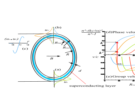
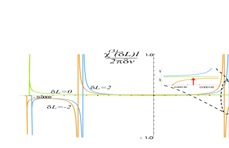
![[Uncaptioned image]](/html/1806.01522/assets/x3.png)
![[Uncaptioned image]](/html/1806.01522/assets/x4.png)
![[Uncaptioned image]](/html/1806.01522/assets/x5.png)
![[Uncaptioned image]](/html/1806.01522/assets/x6.png)
![[Uncaptioned image]](/html/1806.01522/assets/x7.png)
![[Uncaptioned image]](/html/1806.01522/assets/x8.png)
![[Uncaptioned image]](/html/1806.01522/assets/x9.png)
![[Uncaptioned image]](/html/1806.01522/assets/x10.png)