A Fast Algorithm for Maximum Likelihood Estimation of Mixture Proportions Using Sequential Quadratic Programming

Abstract

Maximum likelihood estimation of mixture proportions has a long history, and continues to play an important role in modern statistics, including in development of nonparametric empirical Bayes methods. Maximum likelihood of mixture proportions has traditionally been solved using the expectation maximization (EM) algorithm, but recent work by Koenker & Mizera shows that modern convex optimization techniques—in particular, interior point methods—are substantially faster and more accurate than EM. Here, we develop a new solution based on sequential quadratic programming (SQP). It is substantially faster than the interior point method, and just as accurate. Our approach combines several ideas: first, it solves a reformulation of the original problem; second, it uses an SQP approach to make the best use of the expensive gradient and Hessian computations; third, the SQP iterations are implemented using an active set method to exploit the sparse nature of the quadratic subproblems; fourth, it uses accurate low-rank approximations for more efficient gradient and Hessian computations. We illustrate the benefits of the SQP approach in experiments on synthetic data sets and a large genetic association data set. In large data sets ($n\approx 10^{6}$ observations, $m\approx 10^{3}$ mixture components), our implementation achieves at least 100-fold reduction in runtime compared with a state-of-the-art interior point solver. Our methods are implemented in Julia and in an R package available on CRAN (https://CRAN.R-project.org/package=mixsqp).

Keywords: nonparametric empirical Bayes, nonparametric maximum likelihood, mixture models, convex optimization, sequential quadratic programming, active set methods, rank-revealing QR decomposition

1 Introduction

We consider maximum likelihood estimation of the mixture proportions in a finite mixture model where the component densities are known. The simplest example of this arises when we have independent and identically distributed (i.i.d.) observations $z_{1},\dots,z_{n}$ drawn from a finite mixture distribution with density

$$p(\,\cdot\,|\,x)=\sum_{k=1}^{m}x_{k}g_{k}(\,\cdot\,),$$

where the component densities $g_{k}(\cdot)$ are known and $x=(x_{1},\dots,x_{m})^{T}$ denotes the unknown mixture proportions (non-negative and sum to one). Finding the maximum likelihood estimate (MLE) of $x$ can be formulated as a constrained optimization problem:

minimize $$\quad f(x)\triangleq-\frac{1}{n}\sum_{j=1}^{n}\log\left(\sum_{k=1}^{m}L_{jk}x_{k}\right)$$ (1)

subject to $$\quad x\in\mathcal{S}^{m}\triangleq\big{\{}x:{\textstyle\sum_{k=1}^{m}x_{k}=1},\ x\succeq 0\big{\}},$$

where $L$ is an $n\times m$ matrix with entries $L_{jk}\triangleq g_{k}(z_{j})\geq 0$. This optimization problem arises in many settings—including nonparametric empirical Bayes (EB) computations described later—where observations are not necessarily identically distributed. Here, we develop general methods for solving (1).

Problem (1) is a convex optimization problem and can be solved simply using expectation maximization (EM) (Dempster et al., 1977); see Appendix A. However, the convergence of EM can be intolerably slow (Redner & Walker, 1984; Atkinson, 1992; Salakhutdinov et al., 2003; Varadhan & Roland, 2008); this slow convergence is illustrated evocatively in Koenker & Mizera (2014). Koenker & Mizera (2014) and Koenker & Gu (2017) show that modern convex optimization methods can be substantially faster and more reliable than EM. They demonstrate this by using an interior (IP) method to solve a dual formulation of the original problem. This method is implemented in the KWDual function of the R package REBayes (Koenker & Gu, 2017), which interfaces to the commercial interior point solver MOSEK (Andersen & Andersen, 2000).

In this paper, we provide an even faster algorithm for this problem based on sequential quadratic programming (SQP) (Nocedal & Wright, 2006). The computational gains are greatest in large data sets where the matrix $L\in\mathbb{R}^{n\times m}$ is numerically rank-deficient. Rank deficiency can make the optimization problem harder to solve, even if it is convex (Wright, 1998). As we show, a numerically rank-deficient $L$ often occurs in the nonparametric EB problems that are the primary focus of KWDual. As an example of target problem size, we consider data from a genome-wide association study with $n>10^{6}$ and $m>100$. For such data, our methods are approximately 100 times faster than KWDual (about 10 s vs. 1,000 s). All our methods and numerical experiments are implemented in the Julia programming language (Bezanson et al., 2012), and the source code is available online at https://github.com/stephenslab/mixsqp-paper. Many of our methods are also implemented in an R package, mixsqp, which is available on CRAN (R Core Team, 2017).

2 Motivation: nonparametric empirical Bayes

Estimation of mixture proportions is a fundamental problem in statistics, dating back to at least Pearson (1894). This problem, combined with the need to fit increasingly large data sets, already provides strong motivation for finding efficient scalable algorithms for solving (1). Additionally, we are motivated by recent work on nonparametric approaches to empirical Bayes (EB) estimation in which a finite mixture with a large number of components is used to accurately approximate nonparametric families of prior distributions (Koenker & Mizera, 2014; Stephens, 2016). Here we briefly discuss this motivating application.

We first consider a simple EB approach to solving the “normal means,” or “Gaussian sequence,” problem (Johnstone & Silverman, 2004). For $j=1,\dots,n$, we observe data $z_{j}$ that are noisy observations of some underlying “true” values, $\theta_{j}$, with normally distributed errors of known variance $s_{j}^{2}$,

$$z_{j}\,|\,\theta_{j}\sim N(\theta_{j},s_{j}^{2}).$$ (2)

The EB approach to this problem assumes that $\theta_{j}$ are i.i.d. from some unknown distribution $g$,

$$\theta_{j}\,|\,g\sim g,\quad g\in\mathcal{G},$$ (3)

where $\mathcal{G}$ is some specified class of distributions. The EB approach estimates $g$ by maximizing the (marginal) log-likelihood, which is equivalent to solving:

$$\underset{g\,\in\,\mathcal{G}}{\textrm{minimize}}\;-\frac{1}{n}\sum_{j=1}^{n}\log\left[\int N(z_{j};\theta,s_{j}^{2})\,g(d\theta)\right],$$ (4)

where $N(\,\cdot\,;\mu,\sigma^{2})$ denotes the normal density with mean $\mu$ and variance $\sigma^{2}$. After estimating $g$ by solving (4), posterior statistics are computed for each $j$. Our focus is on the maximization step.

Although one can use simple parametric families for $\mathcal{G}$, in many settings one might prefer to use a more flexible nonparametric family. Examples include:

• $\mathcal{G}=\mathcal{R}$, the set of all real-valued distributions.

• $\mathcal{G}=\mathcal{U}_{0}$, the set of unimodal distributions with a mode at zero. (Extensions to a nonzero mode are straightforward.)

• $\mathcal{G}=\mathcal{SU}_{0}$, the set of symmetric unimodal distributions with a mode at zero.

• $\mathcal{G}=\mathcal{SN}_{0}$, the set of distributions that are scale mixtures of zero-mean normals, which includes several commonly used distributions, such as the $t$ and double-exponential (Laplace) distributions.

The fully nonparametric case, $\mathcal{G}=\mathcal{R}$, is well studied (e.g., Laird 1978; Jiang & Zhang 2009; Brown & Greenshtein 2009; Koenker & Mizera 2014) and it is related to the classic Kiefer-Wolfowitz problem (Kiefer & Wolfowitz, 1956). More constrained examples $\mathcal{G}=\mathcal{U}_{0},\mathcal{SU}_{0},\mathcal{SN}_{0}$ appear in Stephens (2016) (see also Cordy & Thomas 1997), and can be motivated by the desire to shrink estimates towards zero, or to impose some regularity on $g$ without making strong parametric assumptions. For other motivating examples, see the nonparametric approaches to the “compound decision problem” described in Jiang & Zhang (2009) and Koenker & Mizera (2014).

The connection with (1) is that these nonparametric sets can be accurately approximated by a finite mixture with sufficiently large number of components; that is, they can be approximated by

$$\mathcal{G}\triangleq\big{\{}g={\textstyle\sum_{k=1}^{m}x_{k}g_{k}:x\in\mathcal{S}^{m}}\big{\}},$$ (5)

for some choice of distributions $g_{k}$, $k=1,\ldots,m$. The $g_{k}$’s are often called dictionary functions (Aharon et al., 2006). For example:

• $\mathcal{G}=\mathcal{R}$: $g_{k}=\delta_{\mu_{k}}$, where $\delta_{\mu}$ denotes a delta-Dirac point mass at $\mu$, and $\mu_{1},\dots,\mu_{m}\in\mathbb{R}$ is a suitably fine grid of values across the real line.

• $\mathcal{G}=\mathcal{U}_{0}$, $\mathcal{G}=\mathcal{SU}_{0}$: $g_{k}=\text{Unif}[0,a_{k}],\text{Unif}[-a_{k},0]$ or $\text{Unif}[-a_{k},a_{k}]$, where $a_{1},\ldots,a_{m}\in\mathbb{R}^{+}$ is a suitably large and fine grid of values.

• $\mathcal{G}=\mathcal{SN}_{0}$: $g_{k}=N(0,\sigma^{2}_{k})$, where $\sigma_{1}^{2},\ldots,\sigma_{m}^{2}\in\mathbb{R}^{+}$ is a suitably large and fine grid of values.

With these approximations, solving (4) reduces to solving an optimization problem of the form (1), with $L_{jk}=\int N(z_{j};\theta,s_{j}^{2})\,g_{k}(d\theta)$, the convolution of $g_{k}$ with a normal density $N(z_{j};\theta,s_{j}^{2})$.

A common feature of these examples is that they all use a fine grid to approximate a nonparametric family. The result is that many of the distributions $g_{k}$ are similar to one another. Hence, the matrix $L$ is numerically rank deficient and, in our experience, many of its singular values are near floating-point machine precision. We pay particular attention to this property when designing our optimization methods.

The normal means problem is just one example of a broader class of problems with similar features. The general point is that nonparametric problems can often be accurately solved with finite mixtures, resulting in optimization problems of the form (1), typically with moderately large $m$, large $n$, and a numerically rank-deficient $n\times m$ matrix $L$.

3 A new SQP approach

The methods from Koenker & Gu (2017), which are implemented in function KWDual from R package REBayes (Koenker & Gu, 2017) provide, to our knowledge, the best current implementation for solving (1). These methods are based on reformulating (1) as

$$\underset{x\,\in\,\mathcal{S}^{m}}{\textrm{minimize}}\quad-\frac{1}{n}\sum_{j=1}^{n}\log y_{j}\quad\textrm{subject to}\quad Lx=y,$$ (6)

then solving the dual problem (“K-W dual” in Koenker & Mizera 2014),

$$\underset{\nu\,\in\,\mathbb{R}^{m}}{\textrm{minimize}}\quad-\frac{1}{n}\sum_{j=1}^{n}\log\nu_{j}\quad\textrm{subject to}\quad L^{T}\nu\preceq n\mathds{1}_{m},\quad\nu\succeq 0,$$ (7)

where $\mathds{1}_{m}$ is a vector of ones of length $m$. Koenker & Mizera (2014) reported that solving this dual formulation was generally faster than primal formulations in their assessments. Indeed, we also found this to be the case for IP approaches (see Figure 1). For $n\gg m$, however, we believed that the original formulation (1) offered more potential for improvement. In the dual formulation (7), effort depends on $n$ when computing the gradient and Hessian of the objective, when evaluating the constraints, and when computing the Newton step inside the IP algorithm. By contrast, in the primal formulation (1), effort depends on $n$ only in the gradient and Hessian computations; all other evaluations depend on $m$ only.

These considerations motivated the design of our algorithm. It was developed with two key principles in mind: (i) make best possible use of each expensive gradient and Hessian computation in order to minimize the number of gradient and Hessian evaluations; and (ii) reduce the expense of each gradient and Hessian evaluation as much as possible. (We could have avoided Hessian computations by pursuing a first-order optimization method, but we judged that a second-order method would likely be more robust and stable because of the ill-conditioning caused by the numerical rank deficiency of $L$; we briefly investigate the potential of first-order optimization methods in Section 4.3.5.)

To make effective use of each Hessian computation, we apply sequential quadratic programming (Nocedal & Wright, 2006) to a reformulation of the primal problem (1). SQP attempts to make best use of the expensive Hessian computations by finding, at each iteration, the best reduction in a quadratic approximation to the constrained optimization problem.

To reduce the computational cost of each Hessian evaluation, we use a “rank-revealing” QR decomposition of $L$ to exploit the numerical low-rank of $L$ (Golub & Van Loan, 2012). The RRQR matrix decomposition, which need be performed only once, reduces subsequent per-iteration computations so that they depend on the numerical rank, $r$, rather than $m$. In particular, Hessian computations are reduced from $O(nm^{2})$ to $O(nr^{2})$.

In addition to these two key principles, two other design decisions were also important to reduce effort. First, we introduced a reformulation that relaxes the simplex constraint to a less restrictive non-negative one, which simplifies computations. Second, based on initial observations that the primal solution is often sparse, we implemented an active set method (Nocedal & Wright, 2006)—one that estimates which entries of the solution are zero (this is the “active set”)—to solve for the search direction at each iteration of the SQP algorithm. As we show later, an active set approach effectively exploits the solution’s sparsity.

The remaining subsections detail these innovations.

3.1 A reformulation

We transform (1) into a simpler problem with less restrictive non-negative constraints using the following definition and proposition.

Definition 3.1.

A function $\phi:\mathbb{R}_{+}^{m}\rightarrow\mathbb{R}$ is said to be “scale invariant” if for any $c>0$ there exists a $C\in\mathbb{R}$ such that for any $x\in\mathbb{R}_{+}^{m}$ we have $\phi(cx)=\phi(x)-C$.

Proposition 3.2.

Consider the simplex-constrained optimization problem

$$\underset{x\,\in\,\mathcal{S}^{m}}{\rm minimize}\;\phi(x),$$ (8)

where $\phi(x)$ is scale invariant, convex, and nonincreasing with respect to $x$—that is, $x\succeq y$ (the componentwise partial ordering) implies $\phi(x)\leq\phi(y)$ for all $x\in\mathbb{R}_{+}^{m}$. Let $x^{*}(\lambda)$ denote the solution to a Lagrangian relaxation of (8),

$$\underset{x\,\in\,\mathbb{R}^{m}}{\rm minimize}\quad\phi_{\lambda}(x)\triangleq\phi(x)+\lambda\sum_{k=1}^{m}x_{k},\quad\mbox{\rm subject to}\quad x\succeq 0,$$ (9)

for $\lambda>0$. Then $x^{*}\triangleq x^{*}(\lambda)/\sum_{k=1}^{m}x_{k}^{*}(\lambda)$ is a solution to (8).

By setting $\phi$ to $f$, the objective function in (1), this proposition implies that (1) can be solved by instead solving (9) for some $\lambda$. Somewhat surprisingly, in this special case setting $\lambda=1$ yields a solution $x^{*}(\lambda)$ that is already normalized to sum to 1, so $x^{*}=x^{*}(1)$. This result is summarized in the following proposition:

Proposition 3.3.

Solving the target optimization problem (1) is equivalent to solving (9) with $\phi=f$ and $\lambda=1$; that is,

$$\underset{x\,\in\,\mathbb{R}^{m}}{\rm minimize}\quad f^{\star}(x)\triangleq f(x)+\sum_{k=1}^{m}x_{k},\quad\mbox{\rm subject to}\quad x\succeq 0.$$ (10)

The proofs of the propositions are given in the Appendix.

While we focus on the case of $\phi=f$, these ideas should apply to other objective functions so long as they satisfy Definition 3.1; e.g., when $f$ is a composite of “easily differentiable” scale-invariant functions and “thin and tall” linear functions. Many of the algorithmic ideas presented in following sections are applicable to those functions as well. See the Appendix for further discussion.

3.2 Sequential quadratic programming

We solve the reformulated optimization problem (10) using an SQP algorithm with backtracking line search (Nocedal & Wright, 2006). In brief, SQP is an iterative algorithm that, at the $t$-th iteration, computes a second-order approximation of the objective at the feasible point $x^{(t)}$, then determines a search direction $p^{(t)}$ based on the second-order approximation. At iteration $t$, the search direction $p^{(t)}$ is the solution to the following non-negatively-constrained quadratic program:

$$p^{(t)}=\operatorname*{arg\,min}_{p\,\in\,\mathbb{R}^{m}}\textstyle\frac{1}{2}p^{T}H_{t}p+p^{T}g_{t}\quad\textrm{subject to}\quad x^{(t)}+p\succeq 0,$$ (11)

where $g_{t}=\nabla f^{\star}(x^{(t)})$ and $H_{t}=\nabla^{2}f^{\star}(x^{(t)})$ are the gradient and Hessian of $f^{\star}(x)$ at $x^{(t)}$. Henceforth, this is called the “quadratic subproblem.” Computation of the gradient and Hessian is considered in Section 3.3, and solving the quadratic subproblem is discussed in Section 3.4.

After identifying the search direction, $p^{(t)}$, the SQP method performs a backtracking line search to determine a sufficient descent step $x^{(t+1)}=x^{(t)}+\alpha_{t}p^{(t)}$, for $\alpha_{t}\in(0,1]$. In contrast to other projection-based methods such as the projected Newton method (Kim et al., 2010), $x^{(t+1)}$ is guaranteed to be (primal) feasible for all choices of $\alpha_{t}\in(0,1]$ provided that $x^{(t)}$ is feasible. This is due to the linearity of the inequality constraints. As discussed in Nocedal & Wright (2006), the line search will accept unitary steps ($\alpha_{t}=1$) close to the solution and the iterates will achieve quadratic convergence provided the reduced Hessian is positive definite for all co-ordinates outside the optimal active set (the indices that are zero at the solution $x^{*}$). A similar result can be found in Wright (1998).

3.3 Gradient and Hessian evaluations

We now discuss computation of the gradient and Hessian and ways to reduce the burden of computing them.

Lemma 3.4.

For any $x\in\mathbb{R}_{+}^{m}$, the gradient and Hessian of the objective function in (10) are given by

$$\textstyle g=\nabla f^{\star}(x)=-\frac{1}{n}L^{T}d+\mathds{1}_{m},\quad H=\nabla^{2}f^{\star}(x)=\frac{1}{n}L^{T}{\rm diag}(d)^{2}L,$$ (12)

where $\mathds{1}_{m}$ is a vector of ones of length $m$, and $d=(d_{1},\ldots,d_{n})^{T}$ is a column vector with entries $d_{j}=1/(Lx)_{j}$. Further, for any $x\in\mathbb{R}_{+}^{m}$ the following identities hold:

$$x^{T}g=0,\quad x^{T}Hx=1,\quad Hx+g=\mathds{1}_{m}.$$ (13)

Assuming $L$ is not sparse, computing $g$ (and $d$) requires $O(nm)$ multiplications, and computing $H$ requires $O(nm^{2})$ multiplications. The result (13) is easily derived by substitution from (12).

In practice, we find that $L$ is often numerically rank deficient, with (numerical) rank $r<m$. We can exploit this property to reduce computational effort by approximating $L$ with a low-rank matrix. We use either the RRQR decomposition (Golub & Van Loan, 2012) or a truncated singular value decomposition (tSVD) to compute an accurate, low-rank approximation to $L$. Specifically, we use the pqrfact and psvdfact functions from the LowRankApprox Julia package (Ho & Olver, 2018) which implement randomized algorithms based on Halko et al. (2011).

The rank-$r$ QR approximation of $L$ is $\tilde{L}=QRP^{T}$, with $Q\in\mathbb{R}^{n\times r}$, $R\in\mathbb{R}^{r\times m}$ and $P\in\mathbb{R}^{m\times m}$, the permutation matrix. Therefore, a rank-$r$ QR decomposition yields an approximate gradient and Hessian:

$$\tilde{g}=\textstyle-\frac{1}{n}PR^{T}Q^{T}\tilde{d}+\mathds{1}_{m},\quad\tilde{H}=\textstyle\frac{1}{n}PR^{T}Q^{T}\textrm{diag}(\tilde{d})^{2}QRP^{T},$$ (14)

where $\tilde{d}$ is a vector of length $n$ with entries $\tilde{d}_{j}=1/(QRP^{T}x)_{j}$. Corresponding expressions for the tSVD are straightforward to obtain, and are therefore omitted.

Once we have obtained a truncated QR (or SVD) approximation to $L$, the key to reducing the expense of the gradient and Hessian computations is to avoid directly reconstructing $\tilde{L}$. For example, computing $\tilde{g}$ is implemented as $\tilde{g}=-(((\tilde{d}^{T}Q)R)P^{T})^{T}/n+\mathds{1}_{m}$. In this way, all matrix multiplications are a matrix times a vector. The dominant cost in computing $\tilde{H}$ is the product $Q^{T}\textrm{diag}(\tilde{d})^{2}Q$, which requires $O(nr^{2})$ multiplications. Overall, computation is reduced by roughly a factor of $(r/m)^{2}$ per iteration compared with (12). To enjoy this benefit, we pay the one-time cost of factorizing $L$, which, in the regime $n\gg m$, is $O(nmr)$ (Golub & Van Loan, 2012).

3.4 Solving the quadratic subproblem

To find the solution to the quadratic subproblem (11), we set $p^{*}=y^{*}-x^{(t)}$ in which $y^{*}$ is the solution to

$$\underset{y\,\in\,\mathbb{R}^{m}}{\textrm{minimize}}\;\textstyle\frac{1}{2}y^{T}H_{t}y+y^{T}a_{t},\quad\textrm{subject to}\quad y\succeq 0$$ (15)

with $a_{t}=-H_{t}x^{(t)}+g_{t}=2g_{t}-\mathds{1}_{m}$. This problem comes from substituting $y=x^{(t)}+p$ into (11). Solving (15) is easier than (11) due to the simpler form of the inequality constraints.

To solve (15), we implement an active set method following Nocedal & Wright (2006, §16.5). The active set procedure begins at a feasible point $y^{(0)}$ and an initial estimate of the active set, $\mathcal{W}^{(0)}$ (the “working set”), and stops when the iterates $y^{(0)},y^{(1)},y^{(2)},\ldots$ converge to a fixed point of the inequality-constrained quadratic subproblem (15). The initial working set $\mathcal{W}^{(0)}$ and estimate $y^{(0)}$ can be set to predetermined values, or they can be set according to the current SQP iterate, $x^{(t)}$ (this is often called “warm-starting”). We initialized the active set solver to $x^{(0)}=\{\frac{1}{m},\ldots,\frac{1}{m}\}$ in the first iteration of SQP, and used a warm start in subsequent iterations.

The active set method is an iterative method in which the $l$th iteration involves solving an equality-constrained problem,

$$\underset{q\,\in\,\mathbb{R}^{m}}{\textrm{minimize}}\;\textstyle\frac{1}{2}q^{T}H_{t}q+q^{T}b_{l}\quad\textrm{subject to}\quad q_{i}=0,\;\forall i\in\mathcal{W}^{(l)},$$ (16)

where $b_{l}=H_{t}y^{(l)}+a_{t}$. The solution to (16) at the $l$th iteration, $q^{(l)}$, yields a search direction for the next iterate, $y^{(l+1)}$. Computing the solution to (16) reduces to solving a system of linear equations, with one equation for each co-ordinate outside the working set. Therefore, if the number of inactive co-ordinates remains much smaller than $m$, we expect the complexity of the active set step to be much smaller than $O(m^{3})$.

Additional details of the active set implementation, including the updates to the working set in the presence of blocking constraints, are given in the Appendix.

3.5 The “mix-SQP” algorithm

Putting these components together results in Algorithm 1, which we call mix-SQP. We give the algorithm for the case when RRQR is used to approximate $L$; variants of mix-SQP using the truncated SVD, or with no approximation to $L$, are similar. The most complicated part to implement is the active set method; the details of this step are given separately in Algorithm 2 in the Appendix.

Inputs : likelihood matrix, $L\in\mathbb{R}^{n\times m}$; initial estimate, $x^{(0)}\in\mathcal{S}_{m}$; stringency of sufficient decrease condition, $0<\xi<1$ (default is $0.01$); step size reduction in backtracking line search, $0<\rho<1$ (default is $0.5$); SQP convergence tolerance, $\epsilon_{\mathrm{dual}}\geq 0$ (default is $10^{-8}$); convergence tolerance for active set step, $\epsilon_{\mbox{\scriptsize active-set}}\geq 0$ (default is $10^{-10}$).

Output : $x^{(t)}\in\mathbb{R}^{m}$, an estimate of the solution to (1).

Compute RRQR factorization $\{Q,R,P\}$ of $L$;

for t = 0, 1, 2, … do

       Compute approximate gradient $\tilde{g}_{t}$ and Hessian $\tilde{H}_{t}$ at $x^{(t)}$; (see eq. 14)

       $\mathcal{W}\leftarrow\{1,\ldots,m\}\setminus\mathrm{supp}(x^{(t)})$;   (current estimate of working set)

       $y\leftarrow\mbox{\sc mix-active-set}(\tilde{g}_{t},\tilde{H}_{t},\mathcal{W},\epsilon_{\mbox{\scriptsize active-set}})$;   (see Algorithm 2)

       $p^{(t)}\leftarrow y-x^{(t)}$;

       if $\min_{k}(\tilde{g}_{t})_{k}\geq-\epsilon_{\mathrm{dual}}$ then

             stop;   (maximum dual residual of KKT conditions is less than $\epsilon_{\mathrm{dual}}$)

      $\alpha_{t}\leftarrow 1$;   (backtracking line search)

       while $\tilde{f}(x^{(t)}+\alpha_{t}p^{(t)})>\tilde{f}(x^{(t)})+\xi\alpha_{t}\tilde{g}_{t}^{T}p^{(t)}$ do

             $\alpha_{t}\leftarrow\rho\alpha_{t}$;

      $x^{(t+1)}\leftarrow x^{(t)}+\alpha_{t}p^{(t)}$;

Algorithm 1 mix-SQP with RRQR approximation of $L$.

3.6 Practical implementation details

A useful property of problem (1) is that the gradient (12) is unaffected by the “scale” of the problem; for example, if we multiply all entries of $L$ by 100, the gradient remains the same. This property has several practical benefits; for example, the “dual residual,” used to assess convergence of the iterates, is invariant to the scale of $L$.

When we replace $L$ with an approximation, for example $\tilde{L}=QRP^{T}$, we are effectively solving an approximation to (10),

$$\underset{x\,\in\,\mathbb{R}^{m}}{\textrm{minimize}}\quad\tilde{f}(x)\triangleq-\frac{1}{n}\sum_{j=1}^{n}\log\left(\sum_{k=1}^{m}\tilde{L}_{jk}x_{k}\right)+\sum_{k=1}^{m}x_{k}\quad\textrm{subject to}\quad x\succeq 0.$$ (17)

When an approximated likelihood matrix $\tilde{L}$ is used, some entries $\tilde{L}_{jk}$ may have negative values, and thus the terms inside the logarithms, $\sum_{k=1}^{m}\tilde{L}_{jk}x_{k}$, can be slightly below zero at some feasible points. This can occur either due to the randomized nature of the matrix decomposition algorithms we used, or due to the finite precision of the low-rank approximations. This is a critical point to attend to since the logarithm in the objective does not accept negative values, for example when the objective of (17) is evaluated during line search. In principle, this is not a problem so long as the initial point $x^{(0)}$ satisfies $\sum_{k=1}^{m}\tilde{L}_{jk}x_{k}^{(0)}>0$ for all $j$. Indeed, one can refine the problem statement as

$$\underset{x\,\in\,\mathbb{R}^{m}}{\textrm{minimize}}\quad\tilde{f}(x)\quad\textrm{subject to}\quad x\succeq 0,\;\tilde{L}x\succeq 0,$$ (18)

and start with a feasible $x^{(0)}$. In practice, we implemented a simple workaround: we added a small positive constant (typically somewhere between $10^{-8}$ and $10^{-6}$) to all the terms inside the logarithms so as to ensure that they were strictly bounded away from zero for all $x\in\mathcal{S}^{m}$.

4 Numerical experiments

We conducted numerical experiments to compare different methods for solving problems of the form (1). We considered problems of this form that arise from nonparametric EB, with $\mathcal{G}=\mathcal{SN}_{0}$ (Section 2). Our comparisons involved simulating data sets with varying numbers of data points ($n$) and grid sizes ($m$). We also evaluated the methods on a large-scale genetic data set.

4.1 Data sets

For each synthetic data set, we generated $z_{1},\ldots,z_{n}$ independently as

$$z_{j}\,|\,\theta_{j}\sim N(\theta_{j},1),$$

where the means $\theta_{j}$ were i.i.d. random draws from $g$, a heavy-tailed symmetric distribution about zero,

$$g=0.5N(0,1)+0.2t_{4}+0.3t_{6}.$$

Here, $t_{\nu}$ denotes the density of Student’s $t$ distribution with $\nu$ degrees of freedom.

In addition, we used data generated by the GIANT consortium (“Genetic Investigation of ANthropometric Traits”) for investigating the genetic basis of human height (Wood et al., 2014). We used the additive effects on height estimated for $n=\mbox{2,126,678}$ genetic variants (single nucleotide polymorphisms, or SNPs) across the genome. Height is a well-studied example of trait with a complex genetic basis, so the distribution of additive effects is expected to be representative of genetic associations for many other complex traits and diseases (MacArthur et al., 2017). The data consist of the estimated effect sizes, $z_{j}$, and their corresponding standard errors, $s_{j}$. For illustration, we treat the $n$ data points as independent, though in practice there are local correlations between SNPs. See the Appendix for more details on steps taken to download and prepare the GIANT data.

We modeled all data sets using the “adaptive shrinkage” nonparametric EB model from Stephens (2016) (see Sec. 2). The R package ashr, available on CRAN (Stephens et al., 2018), implements various versions of adaptive shrinkage; for our experiments, we re-coded the simplest version of adaptive shrinkage in Julia. This assumes a normal likelihood and a prior that is a finite mixture of zero-centered normals ($\mathcal{G}=\mathcal{SN}_{0}$ in Sec. 2). This leads to matrix entries $L_{jk}=N(z_{j};0,\sigma_{k}^{2}+s_{j}^{2})$, the normal density at $z_{j}$ with zero mean and variance $\sigma_{k}^{2}+s_{j}^{2}$, where $\sigma_{k}^{2}$ is the variance of the $k$th mixture component. For the simulated data, we set $s_{j}=1$; for the GIANT data, we set the $s_{j}$’s to the standard errors provided. The adaptive shrinkage method also requires a grid of variances, $\sigma_{1}^{2},\dots,\sigma_{m}^{2}$. We ran mix-SQP on matrices $L$ with a range of grid sizes, $m$, and for each grid size we used the method from Stephens (2016) to select the grid values. To avoid numerical overflow or underflow, each row of $L$ was computed up to a constant of proportionality such that the largest entry in each row was always 1. (Recall the maximum likelihood estimate is invariant to scaling the rows of $L$.)

4.2 Approaches considered

Most optimization methods tested in our experiments are combinations of the following four elements:

1. Problem formulation: The method either solves the dual (7), simplex-constrained (1), or non-negatively-constrained formulation (10). This choice is indicated by D, S, or NN, respectively.

2. Solver: The optimization problem is solved using an SQP or IP solver. This choice is denoted by SQP and IP, respectively.

3. QP solver: For SQP approaches only, we considered two ways to solve the quadratic subproblem (11): an active set method (see Section 3.4) or an off-the-shelf QP solver (the commercial IP solver MOSEK). We indicate this choice with A or IP, respectively. When the SQP method is not used, we indicate this choice with NA, for “not applicable.”

4. Gradient and Hessian computation: The objective and partial derivatives either are computed exactly (within floating-point precision) by using the full matrix $L$, or approximated using a truncated SVD or RRQR decomposition of $L$ (Section 3.3). We denote this choice by F (for “full matrix”), SVD or QR.

An optimization method is therefore fully specified by

[formulation]-[solver]-[QP solver]-[gradient/Hessian computation].

For example, the mix-SQP method with a RRQR approximation $L$ (Algorithm 1) is written as NN-SQP-A-QR. We also assessed the performance of two methods that do not use second-order information: projected gradient descent (Birgin et al., 2000; Schmidt et al., 2009) and EM (see Appendix A).

All numerical comparisons were run on machines with an Intel Xeon E5-2680v4 (“Broadwell”) processor. Other than the projected gradient method, all methods were run from Julia version 0.6.2 (Bezanson et al., 2012) linked to the OpenBLAS optimized numerical libraries that were distributed with Julia. (The code has also been updated for Julia 1.1.) The KWDual function in R package REBayes (Koenker & Gu, 2017) was called in R 3.4.1 and was interfaced to Julia using the RCall Julia package. The KWDual function used version 8.0 of the MOSEK optimization library. The projected gradient method was run in MATLAB 9.5.0 (2018b) with optimized Intel MKL numerical libraries. Julia source code and scripts implementing the methods compared in our experiments, including Jupyter notebooks illustrating how the methods are used, are available at https://github.com/stephenslab/mixsqp-paper. The mix-SQP method is also implemented as an R package, mixsqp, which is available on CRAN and GitHub (https://github.com/stephenslab/mixsqp).

4.3 Results

4.3.1 Comparison of problem formulations

Figure 1: Runtimes for different formulations of the maximum likelihood estimation problem: dual (7), simplex-constrained (1) and non-negatively-constrained (10). For each problem formulation, we applied an IP or SQP algorithm. As a baseline, we compared against the KWDual function from the REBayes package which solves the dual formulation using MOSEK. Results are from data sets with $m=40$ and $n$ varying from 80 to 40,960. Runtimes are averages over 10 independent simulations.

First, we investigated the benefits of the three problem formulations: the dual form (7), the simplex-constrained form (1) and the non-negatively-constrained form (10). We implemented IP and SQP methods for each of these problem formulations in the JuMP modeling environment (Dunning et al., 2017). We applied these methods to $n\times m$ simulated data sets $L$, with $m=40$ and $n$ ranging from 80 to 40,960. For all SQP solvers, an IP method was used to solve the quadratic subproblems. In summary, we compared solvers $x$-IP-NA-F and $x$-SQP-IP-F, substituting D, S or NN for $x$. In all cases, the commercial solver MOSEK was used to implement the IP method. To provide a benchmark for comparison, we also ran the KWDual method in R, which calls MOSEK.

The results of this experiment are summarized in Figure 1. All runtimes scaled approximately linearly in $n$ (the slope is near 1 on the log-log scale). Of the methods compared, SQP applied to the non-negatively-constrained formulation, NN-SQP-IP-F, consistently provided the fastest solution.

SQP for the non-negatively-constrained formulation was substantially faster than SQP for the simplex-constrained formulation. The former typically required fewer outer iterations, but this does not completely explain the difference in performance—it is possible that the simplex-constrained formulation could be improved with more careful implementation using the JuMP interface.

Of the IP approaches, the fastest was the implementation using the dual formulation. This is consistent with the results of Koenker & Mizera (2014). By contrast, the SQP approach appears to be poorly suited to the dual formulation.

Based on these results, we focused on the non-negatively-constrained formulation for SQP in subsequent comparisons.

4.3.2 Examining the benefits of approximating $L$

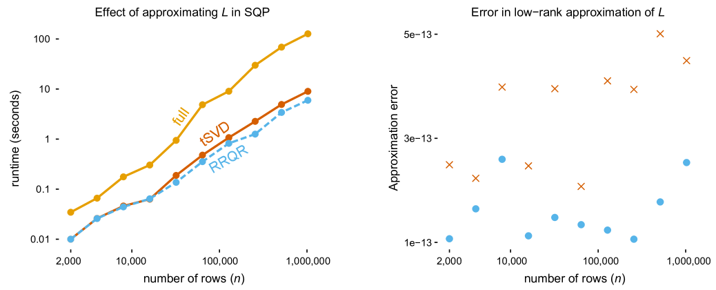
Figure 2: Comparison of SQP methods with and without low-rank approximations to the $n\times m$ matrix, $L$. Left panel: Runtime of the SQP solver using the full matrix (“full”) and using low-rank approximations based on RRQR and tSVD factorizations. Results are from data sets with $m=100$ and varying $n$. Right panel: Reconstruction error in RRQR (blue circles) and tSVD (red crosses); error is computed as $\lVert L-\tilde{L}\rVert_{F}$. All runtimes and errors are averages over 10 simulations.

Next, we investigated the benefits of exploiting the low-rank structure of $L$ (see Section 3.3). We compared the runtime of the SQP method with and without low-rank approximations, RRQR and tSVD; that is, we compared solvers NN-SQP-A-$x$, with $x$ being one of F, QR, or SVD. We applied the three SQP variants to $L$ matrices with varying numbers of rows. We used functions pqrfact and psvdfact from the LowRankApprox Julia package (Ho & Olver, 2018) to compute the RRQR and tSVD factorizations. For both factorizations, we set the relative tolerance to $10^{-10}$.

The left-hand panel in Figure 2 shows that the SQP method with an RRQR and tSVD approximation of $L$ was consistently faster than running SQP with the full matrix, and by a large margin; e.g., at $n=10^{6}$, the runtime was reduced by a factor of over 10. At the chosen tolerance level, these low-rank approximations accurately reconstructed the true $L$ (Figure 2, right-hand panel).

For the largest $n$, SQP with RRQR was slightly faster than SQP with the tSVD. We attribute this mainly to the faster computation of the RRQR factorization. We found that the SQP method took nearly the same solution path regardless of the low-rank approximation method used (results not shown).

Figure 3: Assessment of numeric rank of $L$ and its effect on solution accuracy. Left panel: The ratio of the effective rank $r$ (the rank estimated by pqrfact, with relative tolerance of $10^{-10}$) to $m$, the number of columns. The ratios for the simulated data sets are averages from 10 simulations. Middle panel: $\ell_{1}$-norm of the differences in the solutions from the NN-SQP-A-F and NN-SQP-A-QR solvers applied to the GIANT data set. Right panel: Absolute difference in the objective values at these solutions. For all data sets used in these experiments, $n=\mbox{2,126,678}$.

The demonstrated benefits in using low-rank approximations are explained by the fact that $r$, the effective rank of $L$, was small relative to $m$ in our simulations. To check that this was not a particular feature of our simulations, we applied the same SQP method with RRQR (NN-SQP-A-QR) to the GIANT data set. The ratio $r/m$ in the simulated and genetic data sets is nearly the same (Figure 3, left-hand panel).

We also assessed the impact of using low-rank approximations on the quality of the solutions. For these comparisons, we used the RRQR decomposition and the GIANT data set. In all settings of $m$ tested, the error in the solutions was very small; the $\ell_{1}$-norm in the difference between the solutions with exact and approximate $L$ was close to $10^{-6}$ (Figure 3, middle panel), and the difference in the objectives was always less than $10^{-8}$ in magnitude (Figure 3, right-hand panel).

Figure 4: Effect of QR rank ($r$) on accuracy of SQP solution. Left panel: $\ell_{1}$-norm of the difference in the solutions from the NN-SQP-A-F and NN-SQP-A-QR solvers applied to the same matrix $L$. Right panel: Absolute difference in the objective values at these solutions. All results are averaged over 10 simulated data sets with $n=\mbox{100,000}$, $m=200$ and $r$ ranging from 4 to 20.

To further understand how the RRQR approximation of $L$ affects solution accuracy, we re-ran the SQP solver using QR approximations with different ranks, rather than allow the “rank revealing” QR algorithm to adapt the rank to the data. Figure 4 shows that the quality of the approximate solution varies greatly depending on the rank of the QR decomposition, and that the approximate solution gets very close to the unapproximated solution as the rank is increased (presumably as it approaches the “true” rank of $L$). These results illustrate the importance of allowing the RRQR algorithm to adapt the low-rank factorization to the data.

4.3.3 Comparison of active set and IP solutions to quadratic subproblem

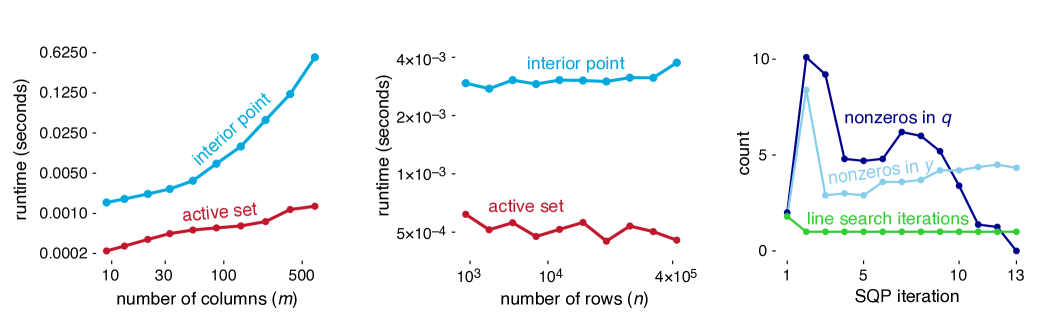
Figure 5: Comparison of active set and interior point methods for solving the SQP quadratic subproblems. Left panel: Runtimes of the active set and IP (MOSEK) methods as $m$ varies, with $n=10^{5}$. Runtimes are averaged over all subproblems solved, and over 10 simulations. Middle panel: Runtimes of the IP and active set methods as $n$ varies, with $m=40$. Right panel: Number of backtracking line searches, and the number of nonzero entries in $q$ and $y$ at each iteration of SQP, averaged over all SQP iterations and all 10 simulations. (Refer to eqs. 15 and 16 for interpreting $q$ and $y$.)

In this set of experiments, we compared different approaches to solving the quadratic subproblems inside the SQP algorithm: an active set method (Section 3.4) and an off-the-shelf IP method (MOSEK); specifically, we compared NN-SQP-A-F against NN-SQP-IP-F. To assess effort, we recorded only the time spent in solving the quadratic subproblems.

The left and middle plots in Figure 5 show that the active set method was consistently faster than the IP method by a factor of roughly 5 or more, with the greatest speedups achieved when $m$ and $n$ were large. For example, when $n=10^{5}$ and $m\approx 500$ in the left-hand plot, the active set solver was over 100 times faster than the IP method on average. The left-hand plot in Figure 5 shows that the complexity of the active set solution to the quadratic subproblem grows linearly in $m$, whereas the complexity of the IP solution grows quadratically. By contrast, the average time required to solve the quadratic subproblems does not depend on $n$ (see Figure 5, middle panel), which could be explained by $n$ having little to no effect on the number of degrees of freedom (sparsity) of the solution $x^{*}$.

We hypothesize that the active set method is faster because the quadratic subproblem iterates and final solution are sparse (see the right-hand plot in Figure 5 for an illustration). Recall that the reformulated problem (10) and the quadratic subproblem (11) have a non-negative constraint, which promotes sparsity.

Based on these results, we infer that the active set method effectively exploits the sparsity of the solution to the quadratic subproblem. We further note that poor conditioning of the Hessian may favor the active set method because it tends to search over sparse solutions where the reduced Hessian is better behaved.

In addition to the runtime improvements of the active set method, another benefit is that it is able to use a good initial estimate when available (“warm starting”), whereas this is difficult to achieve with IP methods. Also, our active set implementation has the advantage that it does not rely on a commercial solver. These qualitative benefits may in fact be more important than performance improvements considering that the fraction of effort spent on solving the quadratic subproblems (either using the active set or IP methods) is relatively small when $n\gg m$.

4.3.4 Comparison of mix-SQP and KWDual

Figure 6: Runtimes of mix-SQP and KWDual (which uses MOSEK) applied to simulated data sets with varying $n$ and $m$, and to the GIANT data set ($n=\mbox{2,126,678}$). All runtimes on simulated data sets were taken as averages over 10 separate simulations. Each timing on the GIANT data set is averaged over 10 independent runs with the same $L$ matrix.

Based on the numerical results above, we concluded that when $n$ and $m$ are large, and $n$ is larger than $m$, the fastest approach is NN-SQP-A-QR. We compared this approach, which we named mix-SQP, against the KWDual function from the R package REBayes (Koenker & Gu, 2017), which is a state-of-the-art solver that interfaces to the commercial software MOSEK (this is D-IP-NA-F). For fair comparison, all timings of KWDual were recorded in R so that communication overhead in passing variables between Julia and R was not factored into the runtimes.

Although R often does not match the performance of Julia, an interactive programming language that can achieve computational performance comparable to C (Bezanson et al., 2012), KWDual is fast because most of the computations are performed by MOSEK, an industry-grade solver made available as an architecture-optimized dynamic library. Therefore, it is significant that our Julia implementation consistently outperformed KWDual in both the simulated and genetic data sets; see Figure 6. For the largest data sets (e.g., $n\approx 10^{6},m=800$), mix-SQP was over 100 times faster than KWDual. Additionally, KWDual runtimes increased more rapidly with $m$ because KWDual did not benefit from the reduced-rank matrix operations.

4.3.5 Assessing the potential for first-order optimization

Figure 7: Progress over time for the EM, projected gradient and mix-SQP methods on two simulated data sets with $n=\mbox{20,000}$ rows and $m=20$ or $m=800$ columns. The vertical axis shows the difference between the value of the log-likelihood, $f(x)\times n$, at the current iterate $x$, and the value of the log-likelihood at the best solution. Each dot corresponds to a single iteration of the algorithm’s main loop.

Our primary focus has been the development of fast methods for solving (1), particularly when $n$ is large. For this reason, we developed a method, mix-SQP, that makes best use of the second-order information to improve convergence. However, it is natural to ask whether mix-SQP is an efficient solution when $m$ is large; the worst-case complexity is $O(m^{3})$ since the active set step requires the solution to a system of linear equations as large as $m\times m$. (In practice, the complexity is often less that this worst case because many of the co-ordinates are zero along the solution path.) Here, we compare mix-SQP against two alternatives that avoid the expense of solving an $m\times m$ linear system: a simple projected gradient algorithm (Schmidt et al., 2009), in which iterates are projected onto the simplex using a fast projection algorithm (Duchi et al., 2008); and EM (Dempster et al., 1977), which can be viewed as a gradient-descent method (Xu & Jordan, 1996).

The projected gradient method was implemented using Mark Schmidt’s MATLAB code. In brief, the projected gradient method is a basic steepest descent algorithm with backtracking line search, in which the steepest descent direction $-\nabla f(x)$ at iterate $x$ is replaced by $\mathcal{P}_{\mathcal{S}}(x-\nabla f(x))-x$, where $\mathcal{P}_{\mathcal{S}}$ denotes the projection onto the feasible set $\mathcal{S}^{m}$. As expected, we found that the gradient descent steps were often poorly scaled, resulting in small step sizes. We kept the default setting of 1 for the initial step size in the backtracking line search. (The spectral gradient method, implemented in the same MATLAB code, is supposed to improve the poor scaling of the steepest descent directions, but we found that it was unstable for the problems considered here.) The EM algorithm, which is very simple (see Appendix A), was implemented in Julia.

To illustrate the convergence behaviour of the first-order methods, we ran the approaches on two simulated data sets and examined the improvement in the solution over time. Our results on a smaller ($\mbox{20,000}\times 20$) and a larger ($\mbox{20,000}\times 800$) data set are shown in Figure 7. Both first-order methods show a similar convergence pattern: initially, they progress rapidly toward the solution, but this convergence slows considerably as they approach the solution; for example, even after running EM and projected gradient for 1,000 iterations on the $\mbox{20,000}\times 800$ data set, the solution remained at least 0.35 log-likelihood units away from the solution obtained by mix-SQP. Among the two first-order methods, the projected gradient method is clearly the better option. Relative to the first-order methods, each iteration of mix-SQP is very costly—initial iterations are especially slow because the iterates contain few zeros at that stage—but mix-SQP is able to maintain its rapid progress as the iterates approach the solution. The benefit of the low-rank (RRQR) approximation in reducing effort is particularly evident in the larger data set.

Although this small experiment is not intended to be a systematic comparison of first-order vs. second-order approaches, it does provide two useful insights. One, second-order information is crucial for obtaining good search directions near the solution. Two, gradient-descent methods are able to rapidly identify good approximate solutions. These two points suggest that more efficient solutions for large data sets, particularly data sets with large $m$, could be achieved using a combination of first-order and second-order approaches, or using quasi-Newton methods.

4.3.6 Profiling adaptive shrinkage computations

Figure 8: Breakdown of computations for the “adaptive shrinkage” EB method (Stephens, 2016), in which the model-fitting step (i.e., maximum likelihood estimation of the mixture proportions) was implemented with either mix-SQP or KWDual (MOSEK). The adaptive shrinkage method was applied to simulated data sets with $m=100$ and varying $n$. All runtimes were averaged over 10 independent simulations. The right-hand panel is a zoomed-in version of the mix-SQP results shown in the left-hand plot.

An initial motivation for this work was our interest in applying a nonparametric EB method, “adaptive shrinkage,” to very large data sets. This EB method involves three steps: (1) likelihood computation; (2) maximum likelihood estimation of the mixture proportions; and (3) posterior computation. When we began this work, the second step, solved using MOSEK, was the computational bottleneck of our R implementation (Stephens et al., 2018); see Figure 8, which reproduces the adaptive shrinkage computations in Julia (aside from KWDual). (To verify that this bottleneck was not greatly impacted by the overhead of calling MOSEK from R inside function KWDual, we also recorded runtime estimates outputted directly by MOSEK, stored in output MSK_DINF_OPTIMIZER_TIME. We found that the overhead was at most 1.5 s, a small fraction of the total model-fitting time under any setting shown in Figure 8. Note all timings of KWDual called from Julia were recorded in R, not Julia.)

When we replaced KWDual with mix-SQP, the model-fitting step no longer dominated the computation time (Figure 8). This result is remarkable considering that the likelihood calculations for the scale mixtures of Gaussians involve relatively simple probability density computations.

5 Conclusions and potential extensions

We have proposed a combination of optimization and linear algebra techniques to accelerate maximum likelihood estimation of mixture proportions. The benefits of our methods are particularly evident at settings in which the number of mixture components, $m$, is moderate (up to several hundred) and the number observations, $n$, is large. In such settings, computing the Hessian is expensive—$O(nm^{2})$ effort—much more so than Cholesky factorization of the Hessian, which is $O(m^{3})$. Based on this insight, we developed a sequential quadratic programming approach that makes best use of the (expensive) gradient and Hessian information, and minimizes the number of times it is calculated. We also used linear algebra techniques, specifically the RRQR factorization, to reduce the computational burden of gradient and Hessian evaluations by exploiting the fact that the matrix $L$ often has a (numerically) low rank. These linear algebra improvements were possible by developing a customized SQP solver, in contrast to the use of a commercial (black-box) optimizer such as MOSEK. Our SQP method also benefits from the use of an active set algorithm to solve the quadratic subproblem, which can take advantage of sparsity in the solution vector. The overall result is that for problems with $n>10^{5}$, mix-SQP can achieve a 100-fold speedup over KWDual, which applies the commercial MOSEK interior point solver to a dual formulation of the problem.

To further reduce the computational effort of optimization in nonparametric EB methods such as Koenker & Mizera (2014) and Stephens (2016), quasi-Newton methods may be fruitful (Nocedal & Wright, 2006). Quasi-Newton methods, including the most popular version, BFGS, approximate $H$ by means of a secant update that employs derivative information without ever computing the Hessian. While such methods may take many more iterations compared with exact Hessian methods, their iterations are $m$ times cheaper—consider that evaluating the gradient (14) is roughly $m$ times cheaper than the Hessian when $n\gg m$—and, under mild conditions, quasi-Newton methods exhibit the fast superlinear convergence of Newton methods when sufficiently close to the solution (Nocedal & Wright, 2006).

Since $n$ is the dominant component of the computational complexity in the problem settings we explored—the gradient and Hessian calculations scale linearly with $n$—another promising direction is the use of stochastic approximation or online learning methods, which can often achieve good solutions using approximate gradient (and Hessian) calculations that do not scale with $n$ (Bottou & Le Cun, 2004; Robbins & Monro, 1951). Among first-order methods, stochastic gradient descent may allow us to avoid linear per-iteration cost in $n$. In the Newton setting, one could explore stochastic quasi-Newton (Byrd et al., 2016) or LiSSA (Agarwal et al., 2016) methods.

As we briefly mentioned in the results above, an appealing feature of SQP approaches is that they can easily be warm started. This is much more difficult for interior point methods (Potra & Wright, 2000). “Warm starting” refers to sequential iterates of a problem becoming sufficiently similar that information about the subproblems that is normally difficult to compute from scratch (“cold”) can be reused as an initial estimate of the solution. The same idea also applies to solving the quadratic subproblems. Since, under general assumptions, the active set settles to its optimal selection before convergence, this suggests that the optimal working set $\mathcal{W}$ for subproblem $\mathcal{P}$ will often provide a good initial guess for the optimal working set $\mathcal{W}^{\star}$ for similar subproblem $\mathcal{P}^{\star}$.

Acknowledgments

This material was based upon work supported by the U.S. Department of Energy, Office of Science, Office of Advanced Scientific Computing Research (ASCR) under Contract DE-AC02-06CH11347. We acknowledge partial NSF funding through awards FP061151-01-PR and CNS-1545046 to MA, and support from NIH grant HG002585 and a grant from the Gordon and Betty Moore Foundation to MS. We thank the staff of the University of Chicago Research Computing Center for providing high-performance computing resources used to implement some of the numerical experiments. We thank Joe Marcus for his help in processing the GIANT data, and other members of the Stephens lab for feedback on the methods and software.

Appendix A EM for maximum-likelihood estimation of mixture proportions

Here we derive the EM algorithm for solving (1). The objective $f(x)$ can be recovered as the log-likelihood (divided by $n$) for $z_{1},\ldots,z_{n}$ drawn i.i.d. from a finite mixture, in which the $x_{k}$’s specify the mixture weights:

$$p(z_{j}\,|\,x)\sim\sum_{k=1}^{m}x_{k}g_{k}(z_{k}),\quad\mbox{for $j=1,\ldots,n$.}$$

The mixture model is equivalently formulated as

$$p(\gamma_{j}=k\,|\,x) =x_{k}$$

$$p(z_{j}\,|\,\gamma_{j}=k) =g_{k}(z_{j}),\quad\mbox{for $j=1,\ldots,n$,}$$

in which we have introduced latent indicator variables $\gamma_{1},\ldots,\gamma_{n}$, with $\gamma_{j}\in\{1,\ldots,m\}$.

Under this augmented model, the expected complete log-likelihood is

$$E[\log p(z\,|\,x,\gamma)] =\sum_{j=1}^{n}E\big{[}\log\big{\{}p(z_{j}\,|\,\gamma_{j})\,p(\gamma_{j}\,|\,x)\big{\}}\big{]}$$

$$=\sum_{j=1}^{n}\sum_{k=1}^{K}\phi_{jk}\log(L_{jk}x_{k}),$$

where $\phi_{jk}$ denotes the posterior probability $p(\gamma_{j}=k\,|\,x,z_{j})$, and $L_{jk}\triangleq g_{k}(z_{j})$. From this expression for the expected complete log-likelihood, the M-step update for the mixture weights works out to

$$x_{k}=\frac{1}{n}\sum_{j=1}^{n}\phi_{jk},$$ (19)

and the E-step consists of computing the posterior probabilities,

$$\phi_{jk}=\frac{L_{jk}x_{k}}{\sum_{k^{\prime}=1}^{m}L_{jk^{\prime}}x_{k^{\prime}}}.$$ (20)

In summary, the EM algorithm for solving (1) is easy to explain and implement: it iteratively updates the posterior probabilities for the current estimate of the mixture weights, following eq. 20 (this is E-step), then updates the mixture weights according to eq. 19 (this is the M-step), until some stopping criterion is met or until some upper limit on the number of iterations is reached.

Appendix B Proofs

Here we provide proofs for Proposition 3.2 and Proposition 3.3.

B.1 Proof of Proposition 3.2

Because of the monotonicity and unboundedness of the objective over the positive orthant, $\mathbb{R}^{m}$, the solution to (8) is preserved if we relax the simplex constraint $\mathcal{S}^{m}=\{x:\mathds{1}^{T}x=1,x\succeq 0\}$ to a set of linear inequality constraints, $\{x:\mathds{1}^{T}x\leq 1,x\succeq 0\}$. Slater’s condition (Boyd & Vandenberghe 2004) is trivially satisfied for both formulations of the simplex constraints, and the feasible set is compact. The solution then satisfies the KKT optimality conditions; i.e., at the solution $x^{*}$ there exists a $\lambda^{*}>0$ and a $\mu^{*}\succeq 0$ such that

$$\nabla\phi(x^{*})+\lambda^{*}\mathds{1}-\mu^{*} =0$$ (21)

$$(\mu^{*})^{T}x^{*} =0$$

$$\mathds{1}^{T}x^{*} =1.$$

We therefore conclude that solving (8) is equivalent to solving

$$\underset{x\,\in\,\mathbb{R}_{+}^{m}}{\textrm{minimize}}\;\phi(x)+\lambda^{*}\big{(}{\textstyle\sum_{k=1}^{m}x_{k}-1}\big{)}.$$ (22)

We claim that for any $\lambda>0$, the solution to the Lagrangian relaxation of the problem,

$$x^{*}(\lambda)=\operatorname*{arg\,min}_{x\in\mathbb{R}_{+}^{m}}\phi(x)+\textstyle\lambda\sum_{k=1}^{m}x_{k},$$

is the same as solution to the original problem up to a constant of proportionality, and the proportionality constant is $\lambda/\lambda^{*}$. So long as $\lambda^{*}>0$, we have that

$$x^{*}(\lambda) =\operatorname*{arg\,min}_{x\,\in\,\mathbb{R}_{+}^{m}}\textstyle\big{\{}\phi(x)+\lambda\sum_{k=1}^{m}x_{k}\big{\}}$$

$$=\operatorname*{arg\,min}_{x\,\in\,\mathbb{R}_{+}^{m}}\textstyle\big{\{}\phi(\frac{\lambda^{\;}}{\lambda^{*}}x)+\lambda^{*}\sum_{k=1}^{m}\frac{\lambda^{\;}}{\lambda^{*}}x_{k}\big{\}}$$

$$=\frac{\lambda^{*}}{\lambda^{\;}}\times\operatorname*{arg\,min}_{x^{\prime}\,\in\,\mathbb{R}_{+}^{m}}\textstyle\big{\{}\phi(x^{\prime})+\lambda^{*}\sum_{k=1}^{m}x_{k}^{\prime}\big{\}}$$

$$=\textstyle\frac{\lambda^{*}}{\lambda^{\;}}x^{*}(\lambda^{*}).$$

The second equality follows from the scale invariance assumption on $\phi(x)$.

Note that $\lambda^{*}=0$ cannot hold at a solution to (8). Suppose that $\lambda^{*}=0$. Then the point $x^{*}$ must satisfy the KKT conditions of the problem in which the equality constraint $\mathds{1}^{T}x=1$ is removed, and it must then be a solution of that problem. Since the objective function decreases as we scale up $x$, such problems clearly are unbounded below and thus cannot have an optimal solution (as scaling $x$ up keeps decreasing the function value while preserving nonnegativity of entries in $x$). Since the solution of (8) must satisfy $\mathds{1}^{T}x=1$, the conclusion follows.

B.2 Proof of Proposition 3.3

The proof follows from the KKT optimality conditions (21). Premultiplying the first set of equations by $(x^{\star})^{T}$, we have that

$$(x^{*})^{T}\nabla f(x^{*})+\lambda^{*}=0.$$

The gradient of the objective in (1) is $\nabla f(x)=-L^{T}d/n$, where $d$ is a vector of length $n$ with entries $d_{j}=1/(Lx)_{j}$. Inserting this expression for the gradient into the above identity yields $\lambda^{*}=1$.

Appendix C Implementation of the active set method

At each iteration of mix-SQP (Algorithm 1), an active set method is used to compute a search direction, $p^{(t)}$. The active set method is given in Algorithm 2. It is adapted from Algorithm 16.3 of Nocedal & Wright (2006). Note that additional logic is needed to handle boundary conditions, such as the case when the working set is empty, and when the working set contains all co-ordinates except one.

Inputs : gradient, $g\in\mathbb{R}^{m}$; Hessian, $H\in\mathbb{R}^{m\times m}$; initial working set, $\mathcal{W}^{(0)}\subseteq\{1,\ldots,m\}$; convergence tolerance, $\epsilon\geq 0$.

Output : $y^{(l)}\in\mathbb{R}^{m}$, an estimate of the solution to (15).

$k\leftarrow m-|W^{(0)}|$;

Set $y_{i}^{(0)}\leftarrow 0,\forall i\in\mathcal{W}^{(0)}$;

Set $y_{i}^{(0)}\leftarrow 1/k,\forall i\notin\mathcal{W}^{(0)}$;

for l = 0, 1, 2, … do

       $b\leftarrow Hy^{(l)}+2g+\mathds{1}_{m}$;   (see eq. 16)

       $q^{(l)}\leftarrow\operatorname*{arg\,min}_{q}q^{T}Hq/2+q^{T}b$ s.t. $q_{i}=0,\forall i\in\mathcal{W}^{(l)}$;   (see eq. 16)

       $\alpha_{l}\leftarrow 1$;

       if $\max_{i}|q_{i}^{(l)}|\leq 0$ then

             if $\min_{i\,\in\,\mathcal{W}^{(l)}}b_{i}\geq-\epsilon$  then

                   stop;   (all Lagrange multipliers in working set are positive)

             $j\leftarrow\operatorname*{arg\,min}_{i\,\in\,\mathcal{W}^{(l)}}b_{i}$;

             $\mathcal{W}^{(l+1)}\leftarrow\mathcal{W}^{(l)}\setminus\{j\}$;   (remove smallest multiplier from active set)

      else

             $j\leftarrow\operatorname*{arg\,min}_{i\,\notin\,\mathcal{W}^{(l)},\,q_{i}^{(l)}<0}-y_{i}^{(l)}/q_{i}^{(l)}$;

             $\alpha_{l}\leftarrow-y_{j}^{(l)}/q_{j}^{(l)}$; (find largest step size retaining feasibility)

             if $\alpha_{l}<1$ then

                   $\mathcal{W}^{(l+1)}\leftarrow\mathcal{W}^{(l)}\cup\{j\}$;   (add blocking constraint to working set)

            

      $y^{(l+1)}\leftarrow y^{(l)}+\alpha_{l}q^{(l)}$;

      

Algorithm 2 mix-active-set: active set method method to compute a search direction for mix-SQP.

Appendix D GIANT data processing details

We retrieved file GIANT_HEIGHT_Wood_et_al_2014_publicrelease_HapMapCeuFreq.txt.gz from the GIANT Project Wiki (http://portals.broadinstitute.org/collaboration/giant). The original tab-delimited text file contained summary statistics—regression coefficient estimates $z_{j}$ and their standard errors $s_{j}$ (columns “b” and “SE” in the text file)—for 2,550,858 SNPs $j$ on chromosomes 1–22 and chromosome X. These summary statistics were computed from a meta-analysis of 79 genome-wide association studies of human height; see Wood et al. (2014) for details about the studies and meta-analysis methods used. We filtered out 39,812 SNPs that were not identified in Phase 3 of the 1000 Genomes Project (Auton et al. 2015), an additional 384,254 SNPs where the coding strand was ambiguous, and 114 more SNPs with alleles that did not match the 1000 Genomes data, for a final data set containing $n=\mbox{2,126,678}$ SNPs. (Note that the signs of the $z_{j}$ estimates were flipped when necessary to align with the 1000 Genomes SNP genotype encodings, although this should have had no effect on our results since the prior is a mixture of zero-centered normals.) The processed GIANT data are included in the accompanying source code repository.

References

- (1)
- Agarwal et al. (2016) Agarwal, N., Bullins, B. & Hazan, E. (2016), ‘Second-order stochastic optimization for machine learning in linear time’, arXiv 1602.03943.
- Aharon et al. (2006) Aharon, M., Elad, M. & Bruckstein, A. (2006), ‘rmK-SVD: an algorithm for designing overcomplete dictionaries for sparse representation’, IEEE Transactions on Signal Processing 54(11), 4311–4322.
- Andersen & Andersen (2000) Andersen, E. D. & Andersen, K. D. (2000), The MOSEK interior point optimizer for linear programming: an implementation of the homogeneous algorithm, in ‘High performance optimization’, Springer, pp. 197–232.
- Atkinson (1992) Atkinson, S. E. (1992), ‘The performance of standard and hybrid EM algorithms for ML estimates of the normal mixture model with censoring’, Journal of Statistical Computation and Simulation 44(1–2), 105–115.
- Auton et al. (2015) Auton, A. et al. (2015), ‘A global reference for human genetic variation’, Nature 526(7571), 68–74.
- Bezanson et al. (2012) Bezanson, J., Karpinski, S., Shah, V. B. & Edelman, A. (2012), ‘Julia: a fast dynamic language for technical computing’, arXiv 1209.5145.
- Birgin et al. (2000) Birgin, E. G., Martínez, J. M. & Raydan, M. (2000), ‘Nonmonotone spectral projected gradient methods on convex sets’, SIAM Journal on Optimization 10(4), 1196–1211.
- Bottou & Le Cun (2004) Bottou, L. & Le Cun, Y. (2004), Large scale online learning, in ‘Advances in Neural Information Processing Systems’, Vol. 16, pp. 217–224.
- Boyd & Vandenberghe (2004) Boyd, S. P. & Vandenberghe, L. (2004), Convex optimization, Cambridge University Press.
- Brown & Greenshtein (2009) Brown, L. D. & Greenshtein, E. (2009), ‘Nonparametric empirical Bayes and compound decision approaches to estimation of a high-dimensional vector of normal means’, Annals of Statistics pp. 1685–1704.
- Byrd et al. (2016) Byrd, R. H., Hansen, S. L., Nocedal, J. & Singer, Y. (2016), ‘A stochastic quasi-Newton method for large-scale optimization’, SIAM Journal on Optimization 26(2), 1008–1031.
- Cordy & Thomas (1997) Cordy, C. B. & Thomas, D. R. (1997), ‘Deconvolution of a distribution function’, Journal of the American Statistical Association 92(440), 1459–1465.
- Dempster et al. (1977) Dempster, A. P., Laird, N. M. & Rubin, D. B. (1977), ‘Maximum likelihood estimation from incomplete data via the EM algorithm’, Journal of the Royal Statistical Society, Series B 39, 1–38.
- Duchi et al. (2008) Duchi, J., Shalev-Shwartz, S., Singer, Y. & Chandra, T. (2008), Efficient projections onto the L1-ball for learning in high dimensions, in ‘Proceedings of the 25th International Conference on Machine Learning’, pp. 272–279.
- Dunning et al. (2017) Dunning, I., Huchette, J. & Lubin, M. (2017), ‘Jump: A modeling language for mathematical optimization’, SIAM Review 59(2), 295–320.
- Golub & Van Loan (2012) Golub, G. H. & Van Loan, C. F. (2012), Matrix Computations, Vol. 3, JHU Press.
- Halko et al. (2011) Halko, N., Martinsson, P.-G. & Tropp, J. A. (2011), ‘Finding structure with randomness: probabilistic algorithms for constructing approximate matrix decompositions’, SIAM Review 53(2), 217–288.
-
Ho & Olver (2018)
Ho, K. L. & Olver, S. (2018),
‘LowRankApprox.jl: fast low-rank matrix approximation in Julia’.
https://doi.org/10.5281/zenodo.1254148 - Jiang & Zhang (2009) Jiang, W. & Zhang, C.-H. (2009), ‘General maximum likelihood empirical bayes estimation of normal means’, Annals of Statistics 37(4), 1647–1684.
- Johnstone & Silverman (2004) Johnstone, I. M. & Silverman, B. W. (2004), ‘Needles and straw in haystacks: empirical Bayes estimates of possibly sparse sequences’, Annals of Statistics 32(4), 1594–1649.
- Kiefer & Wolfowitz (1956) Kiefer, J. & Wolfowitz, J. (1956), ‘Consistency of the maximum likelihood estimator in the presence of infinitely many incidental parameters’, Annals of Mathematical Statistics pp. 887–906.
- Kim et al. (2010) Kim, D., Sra, S. & Dhillon, I. S. (2010), ‘Tackling box-constrained optimization via a new projected quasi-Newton approach’, SIAM Journal on Scientific Computing 32(6), 3548–3563.
- Koenker & Gu (2017) Koenker, R. & Gu, J. (2017), ‘REBayes: an R package for empirical Bayes mixture methods’, Journal of Statistical Software 82(8), 1–26.
- Koenker & Mizera (2014) Koenker, R. & Mizera, I. (2014), ‘Convex optimization, shape constraints, compound decisions, and empirical bayes rules’, Journal of the American Statistical Association 109(506), 674–685.
- Laird (1978) Laird, N. (1978), ‘Nonparametric maximum likelihood estimation of a mixing distribution’, Journal of the American Statistical Association 73(364), 805–811.
- MacArthur et al. (2017) MacArthur, J., Bowler, E., Cerezo, M., Gil, L., Hall, P., Hastings, E., Junkins, H., McMahon, A., Milano, A., Morales, J., Pendlington, Z. M., Welter, D., Burdett, T., Hindorff, L., Flicek, P., Cunningham, F. & Parkinson, H. (2017), ‘The new NHGRI-EBI catalog of published genome-wide association studies (GWAS Catalog)’, Nucleic Acids Research 45(D1), D896–D901.
- Nocedal & Wright (2006) Nocedal, J. & Wright, S. J. (2006), Nonlinear Optimization, Springer, New York, NY.
- Pearson (1894) Pearson, K. (1894), ‘Contributions to the mathematical theory of evolution’, Philosophical Transactions of the Royal Society of London. A 185, 71–110.
- Potra & Wright (2000) Potra, F. A. & Wright, S. J. (2000), ‘Interior-point methods’, Journal of Computational and Applied Mathematics 124(1–2), 281–302.
-
R Core Team (2017)
R Core Team (2017), R: a Language and
Environment for Statistical Computing, R Foundation for Statistical
Computing, Vienna, Austria.
https://www.R-project.org - Redner & Walker (1984) Redner, R. A. & Walker, H. F. (1984), ‘Mixture densities, maximum likelihood and the EM algorithm’, SIAM Review 26(2), 195–239.
- Robbins & Monro (1951) Robbins, H. & Monro, S. (1951), ‘A stochastic approximation method’, Annals of Mathematical Statistics 22(3), 400–407.
- Salakhutdinov et al. (2003) Salakhutdinov, R., Roweis, S. & Ghahramani, Z. (2003), Optimization with EM and expectation-conjugate-gradient, in ‘Proceedings of the 20th International Conference on Machine Learning’, pp. 672–679.
- Schmidt et al. (2009) Schmidt, M., Berg, E., Friedlander, M. & Murphy, K. (2009), Optimizing costly functions with simple constraints: a limited-memory projected quasi-Newton algorithm, in ‘Proceedings of the 12th International Conference on Artificial Intelligence and Statistics’, pp. 456–463.
- Stephens (2016) Stephens, M. (2016), ‘False discovery rates: a new deal’, Biostatistics 18(2), 275–294.
-
Stephens et al. (2018)
Stephens, M., Carbonetto, P., Dai, C., Gerard, D., Lu, M., Sun, L.,
Willwerscheid, J., Xiao, N. & Zeng, M. (2018), ashr: Methods for Adaptive Shrinkage, using
Empirical Bayes.
http://CRAN.R-project.org/package=ashr - Varadhan & Roland (2008) Varadhan, R. & Roland, C. (2008), ‘Simple and globally convergent methods for accelerating the convergence of any EM algorithm’, Scandinavian Journal of Statistics 35(2), 335–353.
- Wood et al. (2014) Wood, A. R., Esko, T., Yang, J., Vedantam, S., Pers, T. H. et al. (2014), ‘Defining the role of common variation in the genomic and biological architecture of adult human height’, Nature Genetics 46(11), 1173––1186.
- Wright (1998) Wright, S. J. (1998), ‘Superlinear convergence of a stabilized sqp method to a degenerate solution’, Computational Optimization and Applications 11(3), 253–275.
- Xu & Jordan (1996) Xu, L. & Jordan, M. I. (1996), ‘On convergence properties of the EM algorithm for Gaussian mixtures’, Neural Computation 8(1), 129–151.
Government License: The submitted manuscript has been created by UChicago Argonne, LLC, Operator of Argonne National Laboratory (“Argonne”). Argonne, a U.S. Department of Energy Office of Science laboratory, is operated under Contract No. DE-AC02-06CH11357. The U.S. Government retains for itself, and others acting on its behalf, a paid-up nonexclusive, irrevocable worldwide license in said article to reproduce, prepare derivative works, distribute copies to the public, and perform publicly and display publicly, by or on behalf of the Government. The Department of Energy will provide public access to these results of federally sponsored research in accordance with the DOE Public Access Plan. http://energy.gov/downloads/doe-public-access-plan.