REORDER: Securing Dynamic-Priority Real-Time Systems Using Schedule Obfuscation

Abstract

The deterministic (timing) behavior of real-time systems (RTS) can be used by adversaries – say, to launch side-channel attacks or even destabilize the system by denying access to critical resources. We propose a protocol (named REORDER) to obfuscate this predictable timing behavior of RTS, especially ones designed using dynamic-priority scheduling algorithms (e.g., EDF). We also present a metric (named “schedule entropy”) that measures the levels of obfuscation introduced into a given real-time system. The REORDER protocol was integrated into the standard Linux real-time scheduler and evaluated on a realistic embedded platform (Raspberry Pi) running the MiBench automotive benchmark workloads. We also demonstrate how designers of RTS can increase the security of their systems and also quantitatively measure the impact (both in terms of security and performance) of using this protocol.

I Introduction

Systems with real-time properties are often engineered to be very predictable[1]. This is necessary for their correct operation and ensuring safety guarantees. Most real-time systems (RTS) are designed to execute repeating jobs (either periodic or sporadic ones) that have explicit “deadline” requirements. Hence, the schedule repeats. Any deviations in timing behavior, for the real-time schedule, can result in the system becoming unstable – thus, adversely affecting the safety of the system. Adversaries can take advantage of this inherent determinism by focusing their attacks on the schedulers in real-time systems [2, 3]. Traditionally, security has always been an afterthought in the design of RTS but that is changing with the advent of high-profile attacks (e.g., denial-of-service attacks using Internet-of-Things devices [4], Stuxnet [5], BlackEnergy [6], etc.). The increase usage of commodity-off-the-shelf (COTS) components along with emerging technologies (e.g., IoT) only exacerbates security problems in RTS.

Hence, the scheduler in RTS is a critical component for maintaining the integrity of the system. In fact, the predictable behavior can be used to improve the security of such systems [7, 8, 9, 10]. On the other hand, there are significant vulnerabilities that adversaries could exploit due to the repeating nature of the real-time task schedules. Consider the spectrum analysis of a $4$-task real-time system (from Example 1 introduced in Section III-A) using discrete Fourier transforms (DFT) (Fig. 1(a)). An adversary can easily reconstruct the execution frequencies (and hence, periods) of all four real-time tasks (annotated by the red arrows) from this information! Such information can be used to launch other attacks – e.g., scheduler side-channels that can then be used to leak critical information [2, 3] or deny critical services, power consumption [11], schedule preemptions [12], electromagnetic (EM) emanations [13] and temperature [14], etc. In fact, defensive techniques for RTS is fairly limited [15, 16, 17, 7, 8, 9, 18, 10].

Obfuscating the schedules, i.e., introducing randomness into the execution patterns of real-time tasks, could be one way to improve the security of RTS. This must be done in a careful manner, so as to not interfere with the timing guarantees that the system can provide, while still introducing diversity into the schedule. Figure 1(b) shows the results of applying our randomization protocol (introduced next) to the same 4-task example mentioned earlier. As the figure shows, DFT analysis applied to an obfuscated schedule results in less regular execution patterns – hence, it is harder to identify the frequencies of two of the tasks (second and third red arrows), thus thwarting some of the potential attacks mentioned earlier.

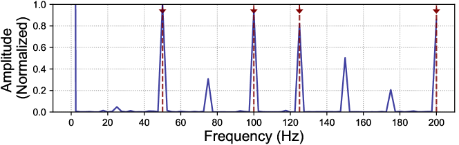
(a) Frequency Spectrum of the EDF Schedule

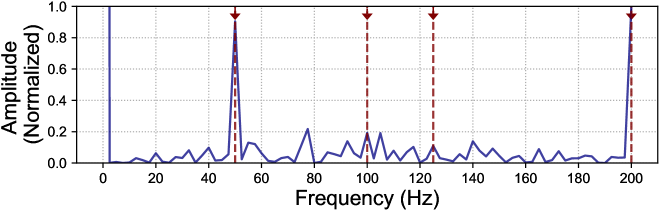
(b) Frequency Spectrum of the Obfuscated Schedule

Fig. 1: Results of the frequency spectrum analysis for execution sequences scheduled by: (a) a deterministic scheduler (e.g., Vanilla EDF) and (b) randomized scheduler (REORDER). A taskset consisting of $4$ periodic tasks is considered and the $4$ arrows (in red) in each plot indicate their true frequencies (i.e., $F_{i}=\tfrac{1}{T_{i}}=\left\{50,100,125,200\right\}$ Hz where $T_{i}$ is the inter-arrival time of the tasks.)

We propose a schedule randomization protocol (Section III) that we named REORDER (REal-time ObfuscateR for Dynamic SchedulER). We achieve this by using bounded priority inversions at runtime (see Section III-A for more details). REORDER obfuscates the earliest deadline first (EDF) scheduling policy [19]; EDF is a dynamic task scheduler that can, theoretically, utilize a CPU to its fullest. It is widely supported by many real-world RTS and operating systems, e.g., Erika Enterprise [20], RTEMS [21], etc. and even Linux [22]. Existing work on protecting real-time schedulers [23, 24] is (a) focused on static scheduling algorithms and (b) inadequate for measuring the effects of obfuscation. Obfuscating the schedules for dynamic priority algorithms such as EDF, to achieve a high level of randomization, is a much harder proposition than that for static algorithms. One important problem is how to bound the time allocated for allowing priority inversions since the job deadlines dynamically change as the execution proceeds. REORDER guarantees that if a given real-time system was schedulable (i.e., meets all of its timing and deadline constraints) by the vanilla EDF scheduler, then the obfuscated schedule will also meet the same guarantees.

A challenge in any security framework is to measure the effectiveness of the solution. In this case, designers of RTS need to estimate the amount of randomness introduced into the real-time schedule by REORDER. Hence, we developed a metric that we named “schedule entropy” (Section IV-A) that measures the amount of obfuscation for each given real-time task set/schedule. Hence, schedule entropy can be used to not just capture the amount of randomness introduced into the system but also compare different obfuscation schemes.

REORDER is implemented in a (real-time) Linux kernel. It was evaluated (Section VI) (a) on a realistic embedded platform (Raspberry Pi) (b) using an automotive benchmark suite (MiBench) [26]. In addition, we also carry out a design-space exploration using synthetic real-time task sets (Section IV-C). This paper makes the following contributions:

• a randomization algorithm that shuffles EDF schedules (Section III-B),

• “schedule entropy” – a new metric to calculate the amount of randomness in the task schedules (Section IV) and

• an implementation of the REORDER algorithm in the Linux kernel (Section VI).

We first present some background information as well as the system and adversary models.

II System and Adversary Model

II-A Background

Standard real-time scheduling theory generally considers periodically executing tasks [27, 19, 28] that models typical real-time control systems. Each task $\tau_{i}$ generates a potentially infinite sequence of jobs and is modeled by the worst-case computation time (WCET) $C_{i}$ and a defined minimum inter-arrival time (i.e., period) $T_{i}$. Also tasks have a strict (relative) deadline $D_{i}$ by which a computation must be finished. Task priorities can be static or dynamic [19]. The optimal static scheme is the RM priority assignment where shorter period implies higher priority. RM can guarantee schedulability of a given set of tasks as long as the total utilization is below $\log 2\approx 69\%$. The overall optimal scheme is EDF – a dynamic-priority algorithm that always picks the job of a task whose deadline is closest. EDF can schedule any set of tasks if the total system utilization does not exceed 100% (e.g., sum of the WCET to period ratio for all tasks in the system is less than unity: $\sum\limits_{\tau_{i}}\tfrac{C_{i}}{T_{i}}<1$).

II-B System Model

Let us consider the problem of scheduling a set of $n$ periodic tasks $\Gamma=\{\tau_{1},\tau_{2},\cdots,\tau_{n}\}$ on a single processor, using the EDF scheduling policy. For simplicity of notation, we use the same symbol $\tau_{i}$ to denote a task’s jobs and use the term task and job interchangeably. We also denote $d_{i}$ as the absolute deadline of $\tau_{i}$ (i.e., deadline of any given job of $\tau_{i}$). We assume cache related preemption delay is negligible compared to WCET of the tasks. We do not consider any precedence or synchronization constraints among tasks and $C_{i},T_{i},D_{i}\in\mathbb{N}^{+},$. We further assume that the tasks have constrained-deadlines, i.e., $D_{i}\leq T_{i}$ and the taskset is schedulable by the EDF scheduling policy, that is the worst-case response time (WCRT) of each task is less than its deadline – since REORDER will be trivially ineffective for an unschedulable taskset.

Under the periodic task model, the schedule produced by any preemptive scheduling policy, for a periodic taskset, is cyclic i.e., the system will repeat the task arrival pattern after an interval that coincides with the taskset’s hyperperiod [29], denoted by $L$. Furthermore, we consider a discrete time model (e.g., integral time units [30]) where system and task parameters are multiples of a time unit.

II-C Adversary Model

We assume that the attackers have access to the timing parameters of the tasksets and also have knowledge of which scheduling policy is being used. The adversary’s objective is to get detailed information about the execution patterns of the real-time tasks and cause greater damage [3, 2], to the system by exploiting the precise schedule information.

As introduced in Section I, the attacker may exploit some side-channels (e.g., power consumption, schedule preemptions, electromagnetic (EM) emanations and temperature) to observe and reconstruct the system schedule [3]. A smart attacker possessing sufficient system information can carry out more advanced attacks under the right conditions, to move the system to an unsafe state. For example, in the now famous Stuxnet attack [5], the malware was remnant in the system for months to collect sensitive information before the main attack. It is possible for a denial-of-service attack to target only a specific service handled by a critical task when the precise schedule information is obtainable. A side-channel attack [31, 32] is also another typical class of attacks that can benefit from such schedule reconstruction attacks. For example, it was shown that the precise schedule information can be exploited to assist in determining the prime and probe [33] instants in a cache side-channel attack to increase the chance of success [2].

We further assume that the scheduler is not compromised and the attacker does not have access to the scheduler. Without this assumption, the attacker can undermine the scheduler or directly obtain the schedule information. Our objective, then, is to reduce the inferability of the schedule for real-time tasksets (and also reduce possibility of other attacks that depend of predictable schedules) while meeting real-time guarantees. The randomness introduced to the schedule increases variations in the system and hence makes attacks that rely on the determinism of the real-time schedule, harder.

III Schedule Randomization Protocol

In this section we describe the REORDER protocol. The focus of our design is such that, even if an observer is able to capture the exact schedule for a period of time (for instance, for a few hyperperiods), REORDER will schedule tasks in a way that succeeding execution traces will show different orders (and timing) of execution for the tasks. The main idea is that at each scheduling point, we pick a random task from the ready queue and schedule it for execution. However such random selection may lead to priority inversions [34] and any arbitrary selection may result in missed deadlines – hence, putting at risk the safety of the system. REORDER solves this problem by allowing bounded priority inversions. It restricts how the schedule may use priority inversions without violating real-time constraints (e.g., deadline) of the tasks. To ensure this, REORDER calculates an “acceptable” priority inversion budget. If the budget is exhausted during execution, then we stop allowing lower priority tasks to execute ahead of the higher priority task that has the empty budget. The following sections present the details of the REORDER protocol.

III-A Randomization with Priority Inversion

A key step that is necessary for randomization is to calculate the maximum amount of time that lower priority jobs, $lp(\tau_{i})$, can execute before $\tau_{i}$. This is much harder in EDF compared to the fixed-priority system (that prior work, TaskShuffler [24], was focused on) due to the dynamic nature of EDF (i.e., the task priority varies at run-time). Therefore we define the worst-case inversion budget (WCIB) $V_{i}$ that represents the maximum amount of time for which a job of some task $\tau_{i}$ with relative deadline $d_{i}$ may be blocked by a job of some task $\tau_{j}\in\Gamma,j\neq i$ with $d_{j}>d_{i}$ (and hence lower relative priority than $\tau_{i}$). In the following we illustrate how we calculate WCIB for each task by utilizing the response time analysis [35, 36] for EDF.

III-A1 Bounding Priority Inversions

The WCRT of $\tau_{i}$ is the maximum time between the arrival of a job of $\tau_{i}$ and its completion. Our idea of bounding priority inversions is to calculate the slack times for each task (e.g., difference between deadline and response time) and allow low priority tasks to execute up to that amount of time. We therefore define the WCIB of $\tau_{i}$ as follows:

$$V_{i}=D_{i}-R_{i}.$$ (1)

where $R_{i}$ represents an upper bound of WCRT (see Appendix -A for the calculation of $R_{i}$). The $V_{i}$ represents the maximum amount of time for which all lower priority jobs $lp(\tau_{i})$ (e.g., $d_{j}>d_{i}$) are allowed to execute while an instance of $\tau_{i}$ is still unfinished without missing its deadline, even in the worst-case scenario. The REORDER protocol guarantees that the real-time constraints are satisfied by bounding priority inversions using $V_{i},\forall\tau_{i}\in\Gamma$. Note that WCIB can be negative for some $\tau_{i}$ – although non-positive WCIB does not attribute that the taskset is unschedulable. At each scheduling point $t$, our idea is to execute some low priority job $\tau_{j}$ with $V_{j}>0$ up to $\min(\widehat{C}_{j}^{t},V_{j})$ additional time-units before it leaves the processor for highest priority job where $\widehat{C}_{j}^{t}$ represents the remaining execution time of $\tau_{j}$ at $t$.

We enforce the WCIB at run-time by maintaining a per-job counter, remaining inversion budget (RIB) $v_{i}$, $0\leq v_{i}\leq V_{i}$. RIB is initialized to $V_{i}$ upon each activation of the jobs of $\tau_{i}$ and decremented for each time unit when $\tau_{i}$ is blocked by any lower priority job. When $v_{i}$ reaches zero no job with absolute deadline greater than $d_{i}$ is allowed to run until $\tau_{i}$ completes. Note that not all the jobs of $\tau_{i}$ may need $C_{i}$ time unit for computation (recall that $C_{i}$ is the worst-case bound of the execution time). If some low-priority job $\tau_{j}$ (e.g., $d_{j}>d_{i}$) that blocks $\tau_{i}$ finishes earlier than $C_{j}$, the RIB $v_{i}$ will not be decreased accordingly.

For a given non-negative WCIB, jobs of $\tau_{i}$ can be delayed for up to $V_{i}$ by priority inversions. The WCRT of $\tau_{i}$ is bounded by $R_{i}+V_{i}=R_{i}+D_{i}-R_{i}=D_{i}$. Hence, $\tau_{i}$ is schedulable with the REORDER protocol and we can assert the following:

Proposition 1.

If $\Gamma$ is schedulable under EDF, WCIB is non-negative for some $\tau_{i}$ and low priority jobs of $\tau_{i}$ do not delay $\tau_{i}$ more than $V_{i}$ then REORDER will not violate the real-time constraints of $\tau_{i}$.

III-A2 Selection of Candidate Jobs for Randomization

As we mentioned earlier, when the run-time counter RIB (i.e., $v_{i}$) reaches zero, no jobs with deadline greater than $d_{i}$ can run while $\tau_{i}$ has an outstanding job. However, lower priority jobs could cause $\tau_{i}$ to miss its deadline by inducing the worst-case interference from the higher priority jobs, i.e., $\forall d_{j}<d_{i}$, due to the chain reaction. Therefore, to preserve the schedulability of such jobs we must prevent it from experiencing such additional delays. We achieve this by the following inversion policy:

$\blacktriangleright$ Randomization Priority Inversion Policy (RPIP): If RIB $v_{i}<0$ for some $\tau_{i}\in\Gamma$, no job $\tau_{j}$ with $d_{j}>d_{i}$ is allowed to run while any of high priority job $\tau_{k}$ with $d_{k}<d_{i}$ has an unfinished job.

In order to enforce RPIP at run-time, at each scheduling decision point, we now define the variable minimum inversion deadline $m_{i}^{t}$ for jobs of $\tau_{i}$ as follows: $m_{i}^{t}=\min\{d_{j}|\tau_{j}\in\mathcal{R}_{\mathcal{Q}}^{t},\leavevmode\nobreak\ d_{j}>d_{i}\wedge v_{j}<0\}.$ where $\mathcal{R}_{\mathcal{Q}}^{t}$ is the ready queue at scheduling point $t$. When there is no such task as $\tau_{j}$, $m_{i}^{t}$ is set to an arbitrarily large (e.g., infinite) deadline. The variable $m_{i}^{t}$ allows us to determine which jobs to exclude from priority inversions. That is, no job that has a higher deadline than $m_{i}^{t}$ can be scheduled as long as $\tau_{i}$ has an unfinished job. Otherwise, the job with relative deadline $m_{i}^{t}$ (not the job $\tau_{i}$) could miss its deadline.

Example 1.

The taskset $\Gamma_{ex1}=\{\tau_{1},\tau_{2},\tau_{3},\tau_{4}\}$ contains the following parameters:

Task	$C_{i}$	$T_{i}=D_{i}$	$V_{i}$
$\tau_{1}$	$4$	$10$	$1$
$\tau_{2}$	$1$	$20$	$-2$
$\tau_{3}$	$1$	$5$	$-2$
$\tau_{4}$	$2$	$12$	$-1$

At $t=0$, $d_{1}=10$, $d_{2}=20$, $d_{3}=5$, $d_{4}=12$. For notational convenience, let us denote $m_{i}^{0}$ as $m_{i}$. Hence $m_{1}=12$, $m_{2}=\infty$, $m_{3}=12$ and $m_{4}=20$. Therefore at $t=0$ the job $\tau_{2}$ and $\tau_{4}$ are not allowed to participate in priority inversion (since $d_{2},d_{4}>m_{i},i\in\{1,3\}$ and $\tau_{1}$, $\tau_{3}$ have not completed.

It can be shown that at any scheduling point $t$ we can enforce RPIP by only examining the inversion deadline of highest priority (e.g., shortest deadline) job, $m_{HP}^{t}$ [24]. Hence, at each scheduling decision, REORDER excludes all ready jobs from the selection that have higher deadline than $m_{HP}^{t}$.

III-B Overview of The Randomization Protocol

The REORDER protocol selects a new job using the following sequence of steps (refer to Algorithm 1 for a formal description) at every scheduling decision point.

• Step 1 (Candidate Selection): At each scheduling point $t$, the REORDER protocol searches for possible candidate jobs (that can be used for priority inversion) in the ready queue. Let us denote $\mathcal{R}_{\mathcal{Q}}^{t}$ as the set of ready jobs, $\tau_{HP}\in\mathcal{R}_{\mathcal{Q}}^{t}$ is the highest priority (i.e., shortest deadline) job in the ready queue and $\mathcal{C}_{\mathcal{L}}^{t}$ represents the set of candidate jobs at some scheduling point $t$.

  • We first check the RIB of the highest priority job $\tau_{HP}\in\mathcal{R}_{\mathcal{Q}}^{t}$. If the RIB is zero, then $\tau_{HP}$ is added to the candidate and REORDER moves to Step 2 since priority inversion is not possible due to its inversion budget being non-positive.

  • When RIB is non-negative (i.e., $v_{HP}>0$), we iterate through the ready queue and add the job $\tau_{i}\in\mathcal{R}_{\mathcal{Q}}^{t}$ to the candidate list $\mathcal{C}_{\mathcal{L}}^{t}$ if its deadline is less than or equal to $m_{HP}^{t}$ (i.e., the minimum inversion deadline of the highest-priority job at scheduling point $t$).

• Step 2 (Randomizing the Schedule): This step selects a random job from the ready queue for execution. The selected job will run until the next scheduling decision point $t^{\prime}$. We randomly pick a job $\tau_{R}$ from $\mathcal{C}_{\mathcal{L}}^{t}$ and set the next scheduling decision point as follows:

  • If $\tau_{R}$ is the highest priority job in the ready queue, the next decision point $t^{\prime}$ will be either when the job finishes or a new job of another task arrives.

  • Otherwise, the next decision will be made at when $\tau_{R}$ completes or the inversion budget expires, that is,

    $$t^{\prime}=t+\min(\widehat{C}_{R}^{t},\widehat{v}),$$ (2)

    unless a new job arrives before time $t^{\prime}$ where $\widehat{v}=\min(v_{j}|\tau_{j}\in\mathcal{R}_{\mathcal{Q}}^{t}\wedge d_{j}<d_{R})$ and $\widehat{C}_{R}^{t}$ represents the remaining execution time of $\tau_{R}$. Note that the variable $\widehat{v}$ is always positive since every job with a higher priority than the selected job has some remaining inversion budget. Otherwise, $\tau_{R}$ would not have been added to the candidate list in Step 1.

We now use a simple example to illustrate our randomization protocol.

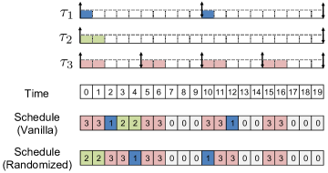
Fig. 2: An instance of schedule randomization protocol for the taskset presented in Example 2. The length of the taskset hyperperiod is $L=20$ and $0$ represents idle time (e.g., when no other tasks are active). The upward and downward arrows represent job activations and deadlines, respectively.

Example 2.

Let us consider the taskset $\Gamma_{ex2}=\{\tau_{1},\tau_{2},\tau_{3}\}$ with following parameters:

Task	$C_{i}$	$T_{i}=D_{i}$	$V_{i}$
$\tau_{1}$	$1$	$10$	$3$
$\tau_{2}$	$2$	$20$	$5$
$\tau_{3}$	$2$	$5$	$3$

The taskset is schedulable by EDF (e.g., $\sum\limits_{\tau_{i}\in\Gamma_{ex2}}\frac{C_{i}}{T_{i}}\leq 1$). The schedule of the vanilla EDF and an instance of randomization protocol is illustrated in Fig. 2. At time $t=0$, all three jobs are in ready queue and have positive inversion budget. Notice that $\tau_{3}$ is the highest priority job, $m_{HP}=\infty$ and all three jobs are in the candidate list. Let the scheduler randomly pick $\tau_{2}$ . From Eq. (2), the next scheduling decision will be taken at $t=0+\min(2,3)=2$. At $t=2$, $v_{1}=v_{3}=1$, $m_{HP}=m_{3}=\infty$ and both $\tau_{1}$ and $\tau_{3}$ are in candidate list. Let $\tau_{3}$ be randomly scheduled (that is also the highest priority job). The next scheduling decision will be at $t=2+2=4$. At $t=4$, only $\tau_{1}$ is active and scheduled (next scheduling decision will be at $t=5$). $\tau_{3}$ is the only active job at time $t=5$ and hence scheduled. At $t=10$, both $\tau_{1}$ and $\tau_{3}$ are active, $m_{3}=m_{HP}=\infty$ and hence both are in candidate list. $\tau_{1}$ is randomly scheduled and the next scheduling point will be at $t=10+1=11$. At $t=11$, only $\tau_{3}$ is active and scheduled. Likewise, $\tau_{3}$ is the only active job at $t=15$ and scheduled.

III-C Unused Time Reclamation

As mentioned earlier, not all the jobs of a task may require worst-case unit of time for its computation. We propose to reclaim this unused time (e.g., difference between WCET and actual execution time) to increase the inversion budget for lower priority jobs. In the case that the (randomly) selected job finishes earlier (i.e., the actual execution time is smaller than its WCET), the unused time that is reserved for this job can be transferred to its lower priority jobs (i.e., those ready jobs that have higher deadlines at the moment) as extra inversion budget. Therefore, when enabling this feature, the RIBs of the lower priority jobs are updated (at the scheduling point $t^{\prime}$ when the selected job $\tau_{R}$ finishes its execution) as follows: $v_{j}=v_{j}+\delta_{R}^{t^{\prime}},\leavevmode\nobreak\ \tau_{j}\in\mathcal{R}_{\mathcal{Q}}^{t^{\prime}}\wedge d_{j}>d_{R}$ where $\delta_{R}^{t^{\prime}}$ represents the unused time over WCET and $\mathcal{R}_{\mathcal{Q}}^{t^{\prime}}$ is the ready queue at time $t^{\prime}$. Note that the real-time constraints (i.e., deadlines) are respected since Eq. 1 for every ready job at time $t^{\prime}$ still holds (i.e., $V_{j}+\delta_{R}^{t^{\prime}}=D_{j}-(R_{j}-\delta_{R}^{t^{\prime}})$) with the unused time transferring.

When there are no tasks in the ready queue (e.g., during slack time), the processor is idle, e.g., nothing is executing in the system. Although REORDER brings variations between the hyperperiods when compared to the vanilla EDF, randomizing only real-time tasks results in the schedule being somewhat predictable since the idle times (i.e., slack) appear in nearly same slots. We address this problem by scrambling the idle times along with the real-time tasks in the next section.

III-D Idle Time Scheduling

One of the limitations of randomizing only the tasks is that the task execution is squeezed between the idle time slots and the latter remain predictable. The work-conserving nature of EDF causes separations between task executions and idle times. Hence some tasks appear at similar places over multiple hyperperiods. One way to address this problem and improve schedule randomness is to idle the processor, intentionally, at random times [24]. We achieve this by considering idle times as instances of an additional task, referred to as the idle task, $\tau_{I}$. Then, the randomization protocol can be applied over the augmented taskset $\Gamma^{\prime}=\Gamma\cup\{\tau_{I}\}$.

It can be noted that $\tau_{I}$ has infinite period, deadline and execution time, and hence always executes with the lowest priority. Hence $\tau_{I}$ can force all other tasks $\tau_{i}\in\Gamma$ to maximally consume their inversion budgets. During randomization the idle task will convert a work-conserving schedule to a non-work-conserving one, but it will not cause any starvation for other tasks. This is because Step 2 of the REORDER protocol (see Section III-B) selects candidate tasks in a way that real-time constraints for all tasks in the system will always be respected. Randomizing the idle task effectively makes tasks appear across wider ranges and thus reduces predictability. As a result, the schedule can be less susceptible to attacks that depend on the predictability of RTS.

III-E Fine-Grained Switching

In prior work [24] researchers proposed to decrease the inferability of the fixed-priority scheduler by randomly yielding a job, early, during execution. As a result the schedule will be fragmented at different time-points and thus will bring more variations across execution windows. Our proposed REORDER protocol can also be modified to incorporate such a feature. Recall that the scheduling decisions in our scheme are made either when: (i) a new job arrives, (ii) a job completes, or (iii) the inversion budget expires (refer to Step 2 in Section III-B). Therefore we can achieve fine-grained switching by modifying the next scheduling decision point $t^{\prime}$ in Eq. (2) as follows: $t^{\prime}=t+\operatorname{rand}(1,\min(\widehat{C}_{R}^{t},\widehat{v}))$ where the function $\operatorname{rand}(a,b)$ outputs a random number between $[a,b]$.

III-F Algorithm

Algorithm 1 formally presents the proposed schedule randomization protocol. This event-driven algorithm executes at the scheduler-level and takes the taskset (with idle time) $\Gamma^{\prime}=\Gamma\cup\{\tau_{I}\}$ as an input. At each scheduling decision point $t$, a ready job is (randomly) selected for scheduling and the next scheduling decision point $t^{\prime}$ is determined.

0:  Augmented task set $\Gamma^{\prime}=\Gamma\cup\{\tau_{I}\}$ and current scheduling point $t$

0:  The randomized schedule $S_{t}$ and the next scheduling point $t^{\prime}$

1:  $\mathcal{R}_{\mathcal{Q}}^{t}:=$ set of ready jobs

2:  Add the highest priority job to the candidate list, i.e., $\mathcal{C}_{\mathcal{L}}^{t}:=\{\mathcal{R}_{\mathcal{Q}}^{HP}\}$

3:  /* Search candidate jobs if the highest priority job has non-zero inversion budget */

4:  if $v_{HP}>0$ then

5:     for each $\tau_{j}\in\mathcal{R}_{\mathcal{Q}}^{t}$ do

6:        if $d_{j}\leq m_{HP}^{t}$ then

7:           $\mathcal{R}_{\mathcal{Q}}^{t}:=\mathcal{R}_{\mathcal{Q}}^{t}\cup\{\tau_{j}\}$ /* add $\tau_{j}$ to candidate list */

8:        end if

9:     end for

10:  end if

11:  if  $\mathcal{C}_{\mathcal{L}}^{t}=\{\mathcal{R}_{\mathcal{Q}}^{HP}\}$  then

12:     /* schedule the highest priority (shortest deadline) job */

13:     $S_{t}:=\mathcal{R}_{\mathcal{Q}}^{HP}$

14:     Set next scheduling point $t^{\prime}:=$ when new job arrives or current job completes

15:  else

16:     /* randomly select a job $\tau_{R}$ from $\mathcal{C}_{\mathcal{L}}^{t}$ */

17:     $S_{t}:=\tau_{R}$

18:     if $\tau_{R}=\mathcal{R}_{\mathcal{Q}}^{HP}$ then

19:        Set next scheduling point $t^{\prime}:=$ when new job arrives or current job completes

20:     else

21:        /* set the next random scheduling point $t^{\prime}$ as a function of current job completion or budget expiration time (unless a new job arrives before $t^{\prime}$) */

22:        $\Delta t:=\operatorname{rand}(1,\min(\widehat{C}_{R}^{t},\widehat{v}))$

23:        Set next scheduling point $t^{\prime}:=t+\Delta t$

24:     end if

25:  end if

26:  /* return the scheduled job and the next scheduling point */

27:  return  $(S_{t},t^{\prime})$

Algorithm 1 Schedule Randomization Protocol

In Lines 3-10, the algorithm first selects the set of candidate jobs $\mathcal{C}_{\mathcal{L}}^{t}$ using the procedure described in Section III-B (see Step 1). If the highest priority job $\mathcal{R}_{\mathcal{Q}}^{HP}$ has negative inversion budget (e.g., $v_{HP}\leq 0$), it will be scheduled for execution (Line 13). Otherwise it schedules a random job from the candidate list (Line 17). If the selected job is the highest priority job, the next scheduling point $t^{\prime}$ is set when the job completes or a new job of another task arrives (Line 14 and 19). If the selected job is not the highest priority one, the algorithm selects $t^{\prime}$ when the current inversion budget expires, unless the job completes or a new job arrives before $t^{\prime}$ (Line 23).

The algorithm iterates over the jobs in the current ready queue $\mathcal{R}_{\mathcal{Q}}^{t}$ once and makes a single draw from the candidate list $\mathcal{C}_{\mathcal{L}}^{t}\subseteq\mathcal{R}_{\mathcal{Q}}^{t}$. Assuming a single draw from a uniform distribution (Line 17 and 22) takes no more than $O(|\mathcal{R}_{\mathcal{Q}}^{t}|)$, the complexity of each instance of the algorithm is $O(|\mathcal{R}_{\mathcal{Q}}^{t}|)$ .

IV Schedule Entropy: A Measure of Randomness

While the mechanisms presented in Algorithm 1 obfuscates the inherent determinism in conventional dynamic-priority schedules, we still need to quantify the randomness that has been introduced into the schedule. This can be addressed by analyzing the schedule entropy that measures the randomness (or unpredictability) in the real-time schedule. Since prior entropy calculations do not capture the randomness of a schedule correctly (refer to Appendix -B for details) we now introduce a better approach to measure the schedule entropy.

IV-A Entropy of a REORDER Schedule

The proposed concept is based on a statistical model – approximate entropy (ApEn) [37] that is used to evaluate the amount of regularity in time series data. Let us consider $K>1$ hyperperiods for a taskset $\Gamma$ (with hyperperiod-length $L$) that is represented as $K$ vectors of length $L$ as follows: $[s_{0}^{1},\cdots,s_{L-1}^{1}],\cdots,[s_{0}^{K},\cdots,s_{L-1}^{K}]$. Each vector includes $L$ intervals of length $m$ of the form $X=\left[s_{t\!\!\!\mod L},s_{(t+1)\!\!\!\mod L},\cdots,s_{(t+m-1)\!\!\!\mod L}\right]$, $0\leq t\leq L-1$ and hence, we have total $\lambda=KL$ number of intervals of length $m$. Let us consider $X_{t}^{k}(m)=\left[s^{k}_{t\!\!\!\mod L},s^{k}_{(t+1)\!\!\!\mod L},\cdots,s^{k}_{(t+m-1)\!\!\!\mod L}\right]$ as the interval of size $m$ starting from $s_{t}^{k}$ on the $k$-th hyperperiod where $0\leq t\leq L-1$ and $1\leq k\leq K$. For all intervals $X^{(k)}_{t}(m)$, let us define the following variable: $C_{t}^{k}\coloneqq\frac{1}{K}\left|\{k^{\prime}:\delta(X^{k}_{t}(m),X^{k^{\prime}}_{t}(m))\leq\pi,\leavevmode\nobreak\ 1\leq k^{\prime}\leq K\}\right|,$ where $\delta(\cdot,\cdot)$ denotes the dissimilarity between two intervals of different hyperperiod, $\pi$ is a given dissimilarity threshold and $|\cdot|$ represents the set cardinality. We use Hamming distance [38] to evaluate the dissimilarity between intervals – since this a relatively simple and widely used dissimilarity measure. For two vectors $U=[u_{i}]_{1\leq i\leq m}$ and $V=[v_{i}]_{1\leq i\leq m}$ of size $m$, Hamming distance is calculated as follows: $\delta(U,V)=\sum\limits_{i=1}^{m}\mathbb{I}(u_{i}\neq v_{i})$, where $\mathbb{I}(\cdot)$ is the indicator function that equals $1$ if the condition $(\cdot)$ is satisfied or $0$ otherwise. Notice that, $C_{t}^{k}$ represents the number of intervals of length $m$ starting from $s_{t}^{k^{\prime}}$, $1\leq k^{\prime}\leq K$ with dissimilarity (in terms of Hamming distance) less than or equal to $r$ from $X^{k}_{t}(m)$ and normalized by the number of observed hyperperiods (i.e., $K$).

Let us now define the variable $\eta_{t}$ as an estimation of the entropy of variable $X_{t}^{k}(m)$, i.e., an estimation of the entropy of a vector that starts from slot $t$ with length $m$ as follows: $\eta_{t}=-\frac{1}{K}\sum\limits_{k=1}^{K}\log_{2}C^{k}_{t}.$ Therefore for a given interval length $1\leq m\leq L$ and dissimilarity threshold $\pi$, the randomness (entropy) of a schedule observed over $K$ hyperperiods is given by the following equation: $\widehat{H}(\mathcal{S}^{k},m,\pi,K)=\frac{1}{m}\sum\limits_{t=0}^{L-1}\eta_{t}.$ Notice that, for a deterministic scheduler (e.g., when all the jobs of the tasks take WCET for computation for vanilla EDF) the schedule entropy $\widehat{H}(\mathcal{S}^{k},m,\pi,K)$ will be equal to zero (i.e., there is no randomness, as expected).

IV-B Interpretation of Entropy

The schedule entropy depicts the randomness for a given schedule. When comparing the entropies of two schedule sequences with equal lengths, a higher value implies that more variations are introduced in each time slot and the chance for a task appearing at the same time slot in every hyperperiod is smaller. Consider the taskset presented in Example 1 as an example – the schedule entropies are $6.12$ and $9.49$ when scheduled by vanilla EDF and REORDER, respectively. As we can see from the frequency spectrum of the two schedule sequences (Fig. 1), the higher randomness reduces the determinism in the schedule and some periods become unidentifiable from the spectral analysis.

Other methods, such as side-channel attacks, also suffer since the victim tasks can potentially appear in larger ranges of executions. Such attacks typically require “prepping” (e.g., prime and probe [33]) of the system and the closer this is done to the actual execution of the victim task, the better it is for the adversary. With increasing entropy values, the attacker has lesser precision in narrowing the exact arrival times for the victim task(s) and hence, experiences more noise in measurements. Similarly, covert channels [39] will also suffer since the expected execution order of tasks is broken due to the randomization – hence, higher entropy values result in larger variations from the “expected” covert channel.

IV-C Evaluation of Schedule Entropy

We now evaluate the REORDER protocol with synthetic workloads. This is to understand the degree of randomness introduced into the schedule and we use the schedule entropy calculations from Section IV-A. The evaluation of scheduling overhead on a real platform is presented in Section VI.

IV-C1 Simulation Setup

We used the parameters similar to that in earlier research [8, 24, 40, 41]. The tasksets were grouped into base-utilization buckets (e.g., total sum of the task utilizations) from $[0.01+0.1\cdot i,0.1+0.1\cdot i]$ where $i\in\mathbb{Z}\wedge 0\leq i<9$. Each base-utilization group contained $250$ tasksets and each of which had $[3,10]$ tasks. We only considered tasksets that were schedulable by EDF.

For a given base-utilization bucket, the utilization $U_{i}$ of individual tasks were generated from a uniform distribution using the UUniFast [42] algorithm. The period of each task was greater than $10$ with a divisor of $100$. This allowed us to set a common hyperperiod (e.g., $L=100$) for all the tasksets. We assumed that the deadlines are implicit, e.g., $D_{i}=T_{i},\leavevmode\nobreak\ \forall\tau_{i}$. The execution time $C_{i}$ for each of the tasks in the taskset was computed using the generated period and utilization: $C_{i}=\lceil U_{i}T_{i}\rceil$. The execution time of each job of $\tau_{i}$ was randomly selected from $\lceil\alpha\cdot C_{i}\rceil$ where $\alpha=[0.5,1]$. The interval window size was $m=\lceil 0.35L\rceil$ and the dissimilarity threshold $\pi$, $0.1L$ (Appendix -C). For each schedulable taskset, we observed the schedule for $K=100$ hyperperiods.

IV-C2 Results

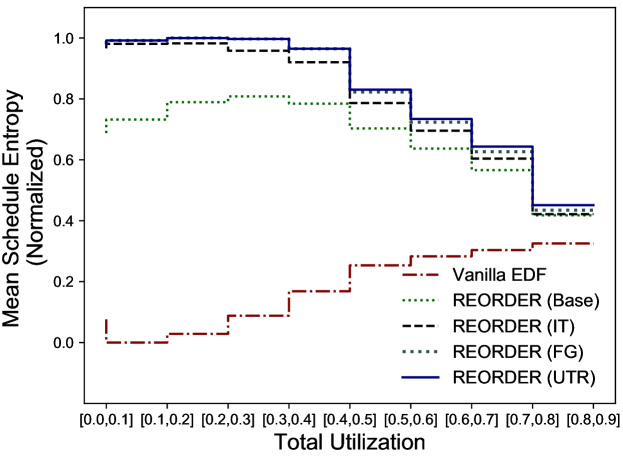
Fig. 3: The average entropy of the system with varying total utilization for different randomization schemes. The REORDER schedule shows maximum randomness (e.g., entropy) in the low-to-medium base-utilization (e.g., $<0.7$).

We now evaluate how much randomness (viz.,  unpredictability) the REORDER protocol incurs w.r.t. vanilla EDF using the following schemes:

• REORDER (Base): only tasks are randomized;

• REORDER (IT): randomization with augmented tasksets (e.g., including idle time randomization);

• REORDER (FT): fine-grained switching for augmented taskset (e.g., yielding tasks at random points); and

• REORDER (UTR): randomization with fine-grain scheduling and unused time reclamation.

In these experiments we focus on observing the average behavior of randomization schemes. In Fig. 3 we present the average schedule entropy of vanilla EDF (e.g., no randomization) along with different randomization schemes.

The X-axis of Fig. 3 shows the total system utilization. The Y-axis represents mean schedule entropy (normalized to $1$), e.g., $\widehat{H}_{mean}(\cdot)=\tfrac{1}{\hat{n}_{s}}\sum\limits_{i=1}^{\hat{n}_{s}}\widehat{H}_{i}(\cdot)$, where $\hat{n}_{s}$ represents the number of schedulable tasksets for a given base-utilization group and $\widehat{H}_{i}(\cdot)$ is the entropy of taskset $i$. For higher utilizations entropy for vanilla EDF increases since the schedule across multiple hyperperiods becomes different because of less slack (e.g., idle times). As we can see from this figure, the randomization protocol significantly increases schedule entropy. The idle time randomization with fine-grained scheduling and unused time reclamation (e.g., REORDER (UTR)) significantly improves the entropy over base randomization. Note that for higher utilization the improvement is marginal. This is due the fact that for higher utilization, the system does not have enough slack (e.g., idle times) to randomize much – and hence all three schemes show similar results (in terms of schedule entropy). As the utilization increases (e.g., lesser slack), there are very few candidate jobs for priority inversions because of higher load. Hence, the entropy (i.e., randomness) drops – albeit the schedule is still less predictable compared to the vanilla EDF (since the mean entropy is greater than entropy of EDF).

Another way to observe the schedule randomness is to measure the ranges within which each task can appear. A wider range implies that is is harder to predict when a task executes. In this experiment we measured the first and the last time slots where a job of each task $\tau_{i}$ appears and used the difference between them as the range of execution for $\tau_{i}$ (denoted as $w_{i}$). In Fig. 4 we show the ratio of execution range to deadline (e.g., $\tfrac{w_{i}}{D_{i}}\leq 1$) of the tasks. The X-axis of the figure shows total utilization and Y-axis represents the geometric mean of the task execution range to deadline ratios in each taskset.

For low utilization situations, tasks appear within narrow ranges because of the work-conserving nature of the EDF algorithm. With increasing utilization the ranges become wider. This is because the worst-case response times of tasks (particularly, for lower priority tasks) increases due to the higher loads. For lower utilization, the system is dominated by slack times and hence randomizing tasks do not improve the execution range compared to vanilla EDF. This is because some (low-priority) jobs finish earlier due to priority inversions and hence the response time of those jobs is actually lower than the EDF scheme. As a result mean ratio for REORDER decreases. As the figure shows, for higher utilization (e.g., utilization greater than $0.4$) tasks appear in wider ranges (e.g., higher mean ratio) when REORDER is enabled. This is due to the fact that priority inversions with REORDER (FT/UTR) increase task response times (especially for higher priority tasks). Besides, inverting the priority can also move lower priority jobs closer to their release times, thus widening the execution range. Since the tasks with REORDER appear in wider ranges this also prevents an attacker from triggering side channel attacks as we mentioned in Section IV-B.

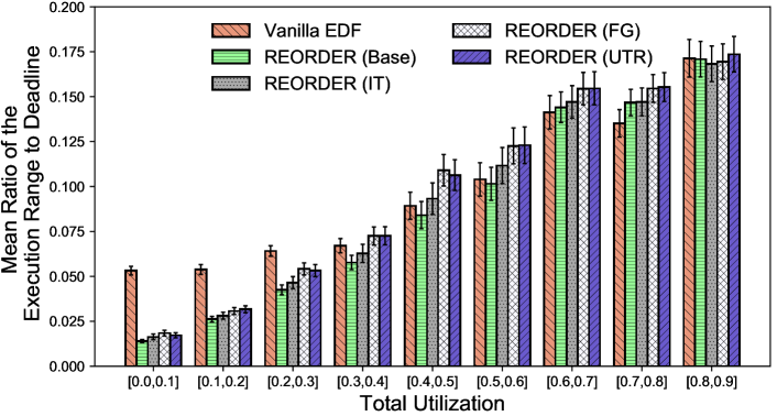
Fig. 4: The geometric mean of the execution range to the deadline ratio. For REORDER the mean ratio is higher when utilization is greater than $0.4$ – that implies the tasks appear in wider ranges and hence it is harder to infer the actual execution time.

V Implementation

We implemented REORDER in a real-time Linux kernel running on a realistic embedded platform to validate its usability and to evaluate its overhead. To this end we also measure the overheads by comparing this to an existing vanilla EDF scheduler. In this section we provide platform information and a high level overview of the implementation. We have open-sourced our implementation and make it available on an anonymized public repository [25]. The platform information and configurations are summarized in Table I.

Table I: Summary of the Implementation Platform

Artifact	Parameters
Platform	ARM Cortex-A53 (Raspberry Pi 3)
System Configuration	1.2 GHz 64-bit processor, 1 GB RAM
Operating System	Debian Linux (Raspbian)
Kernel Version	Linux Kernel 4.9.48
Real-time Patch	PREEMPT_RT 4.9.47-rt37
Kernel Configuration ($\mathtt{make\leavevmode\nobreak\ defconfig}$)	$\mathtt{CONFIG\_SMP}$ disabled $\mathtt{CONFIG\_PREEMPT\_RT\_FULL}$ enabled
Boot Commands	$\mathtt{maxcpus}$=1
Run-time Variables	$\mathtt{sched\_rt\_runtime\_us}$=$-$1
	$\mathtt{scaling\_governor}$=$\mathtt{performance}$
MiBench Applications	Security: $\mathtt{sha,blowfish}$
	Consumer: $\mathtt{typeset}$
	Automotive: $\mathtt{basicmath,bitcount,}$
	$\mathtt{qsort,susan}$

V-A Platform and Operating System

We used a Raspberry Pi 3 (RPi3) Model B development board as the base platform for our implementation. The RPi3 is equipped with a 1.2 GHz 64-bit quad-core ARM Cortex-A53 CPU developed on top of Broadcom BCM2837 SoC (System-on-Chip). RPi3 runs on a vendor-supported open-source operating system, Raspbian (a variant of Debian Linux). We forked the Raspbian kernel and modified it (refer to the following sections) to implement the REORDER protocol. Since we focus on the single core EDF scheduler in this paper, the multi-core functionality of RPi3 was deactivated by disabling the $\mathtt{CONFIG\_SMP}$ flag during the Linux kernel compilation phase. The boot command file was also set with $\mathtt{maxcpus}=1$ to further ensure the single core usage.

V-B Real-time Environment

The mainline Linux kernel does not provide any hard real-time guarantees even with the custom scheduling policies (e.g., $\mathtt{SCHED\_FIFO}$, $\mathtt{SCHED\_RR}$). However the Real-Time Linux (RTL) Collaborative Project [43] maintains a kernel (based on the mainline Linux kernel) for real-time purposes. This patched kernel (known as the PREEMPT_RT) ensures real-time behavior by making the scheduler fully preemptable. In this paper, we applied the PREEMPT_RT patch on top of vanilla Raspbian (kernel version 4.9.48) to enable the real-time functionality. To further enable the fully preemptive functionality from the PREEMPT_RT patch, the $\mathtt{CONFIG\_PREEMPT\_RT\_FULL}$ flag was enabled during the kernel compilation phase. Furthermore, the system variable /proc/sys/kernel/sched_rt_runtime_us was set to $-1$ to disable the throttling of the real-time scheduler. This setting allowed the real-time tasks to use up the entire $100\%$ CPU utilization if required. Also, the active core’s scaling_governor was set to “performance” mode to disable dynamic frequency scaling during the experiments.

V-C Vanilla EDF Scheduler

Since Linux kernel version 3.14, an EDF implementation ($\mathtt{SCHED\_DEADLINE}$) is available in the kernel[22]. Since our PREEMPT_RT patched kernel supports $\mathtt{SCHED\_DEADLINE}$, we used this as the baseline EDF implementation and extended the scheduler to implement the REORDER protocol.

In Linux the system call $\mathtt{sched\_setattr()}$ is invoked to configure the scheduling policy for a given process. By design, $\mathtt{SCHED\_DEADLINE}$ has the highest priority among all the supported scheduling policies (e.g., $\mathtt{SCHED\_NORMAL}$, $\mathtt{SCHED\_FIFO}$ and $\mathtt{SCHED\_RR}$). It’s also worth noting that the Linux kernel maintains a separate run queue for $\mathtt{SCHED\_DEADLINE}$ (i.e., $\mathtt{struct\ dl\_rq}$). Therefore, it is possible to extend $\mathtt{SCHED\_DEADLINE}$ while keeping other scheduling policies untouched. Note that this vanilla EDF scheduler is also used as a base for comparison with the REORDER protocol. The experimental results are presented in Section VI.

V-D Implementation of REORDER

V-D1 Task/Job-specific Variables

The Linux kernel defines a structure, $\mathtt{struct\ sched\_dl\_entity}$, dedicated to $\mathtt{SCHED\_DEADLINE}$, to store task and job-related variables (both run-time and static variables). They include typical EDF task parameters (e.g., period, deadline and WCET).

To implement REORDER we added two additional variables, named $\mathtt{reorder\_wcib}$ and $\mathtt{reorder\_rib}$, both $\mathtt{s64}$ (signed 64 bit integer) type variables, to store the WCIB for the task and to track the RIB for the task’s active job at any given moment, respectively. Each task’s $\mathtt{reorder\_wcib}$ is initialized and updated when a new task is created. The job-specific run-time variable, $\mathtt{reorder\_rib}$, is initialized to the precomputed $\mathtt{reorder\_wcib}$ every time when a new job arrives. During run-time, the inversion budget was updated (i.e., decreased by the elapsed time in the case of priority inversion) along with other $\mathtt{SCHED\_DEADLINE}$ run-time variables in the function $\mathtt{update\_curr\_dl()}$. It is used to determine whether the inversion budget was consumed and a random selection of a job was allowed at a scheduling point.

In our implementations we did not use any external libraries and only used the built-in kernel functions. The following listing shows a part of the existing variables as well as the newly added ones (the highlighted lines). Other variables added for the REORDER protocol are shown in Appendix -D.

⬇

struct sched_dl_entity {

/* task specific parameters */

u64 dl_runtime; // WCET

u64 dl_deadline; // relative deadline

u64 dl_period; // period

s64 reorder_wcib; // worst-case inversion budget

⬇

/* task instance (job) specific parameters */

s64 runtime; // remaining runtime

u64 deadline; // absolute deadline

s64 reorder_rib; // remaining inversion budget

....

/* Other variables are omitted for readability. */

};

V-D2 Task Selection Function

The REORDER protocol was implemented as a function, named $\mathtt{pick\_rad\_next\_dl\_entity()}$, that selects a task and sets the next scheduling point based on the REORDER algorithm. It replaces the original $\mathtt{SCHED\_DEADLINE}$ function, $\mathtt{pick\_next\_dl\_entity()}$ (i.e., one that picks the task that has the next absolute deadline from the run queue, viz., the leftmost node in the scheduler’s red-black tree). This function is indirectly called by the main scheduler function $\mathtt{\_\_schedule()}$ when the next task for execution is needed.

V-D3 Randomization Function

We used the built-in random number generator in the kernel. It supports the system call $\mathtt{get\_random\_bytes()}$ defined in linux/random.h. It is used by the function $\mathtt{pick\_rad\_next\_dl\_entity()}$ to select a random task and a random execution interval for the next scheduling point as explained in Algorithm 1.

V-D4 Schedule Timer

A high-resolution timer (i.e., $\mathtt{struct\ hrtimer}$) was used to trigger the additional scheduling points introduced by the REORDER protocol, as described in Algorithm 1 (Line 22 and 23). Since this timer is a scheduler-specific timer, it is stored in $\mathtt{dl\_rq}$, as $\mathtt{reorder\_pi\_timer}$. It is worth noting that $\mathtt{hrtimer}$ is also used by $\mathtt{SCHED\_DEADLINE}$ to enforce the task periods.

V-D5 Idle Time Scheduling

As introduced in Section III-D, idle times are considered when the idle time scheduling scheme is deployed. In our Linux kernel implementation, we utilized the native idle task maintained under the $\mathtt{SCHED\_IDLE}$ scheduler for this purpose. The REORDER protocol yields its scheduling opportunities (to other schedulers such as $\mathtt{SCHED\_IDLE}$) if $\tau_{I}$, the idle task in the REORDER protocol, is selected and running. The subsequent scheduling point is enforced by $\mathtt{reorder\_pi\_timer}$.

VI Evaluation

In this section, we evaluate REORDER using a prototype implemented on an embedded platform (i.e., RPi3) running the real-time Linux kernel. We mainly focus on overheads for computing and selecting a task at each scheduling point. Recall that our implementation is based on the vanilla EDF scheduler, $\mathtt{SCHED\_DEADLINE}$, on Linux. Therefore, we evaluate the overheads of the REORDER protocol by comparing them with $\mathtt{SCHED\_DEADLINE}$. The key observations from our performance evaluation results are summarized below.

• REORDER works in practice on realistic embedded RTS and is able to meet the real-time guarantees.

• The randomization logic adds minimal scheduling overhead in Linux kernel (Fig. 5). This overhead is arguably very small w.r.t. the task execution time (Fig. 6).

VI-1 Experimental Setup

We use the RPi3 platform as introduced in Section V. The operating system is patched and configured to enable the real-time capability, as shown in Table I. To keep the vanilla EDF unpolluted from our implementation, we used two separately compiled kernels during the experiments. In the vanilla EDF kernel, the scheduling functions remained untouched. Only the necessary code to benchmark the overhead were added. Note that PREEMPT_RT real-time patch was still applied on this kernel.

We used a mixture of MiBench benchmark automotive programs [26] and synthetically generated tasks. The goal of the experiments was to evaluate the performance on both real and synthetic workloads on a real platform. A total of $800$ tasksets were tested. Each taskset was configured with the number of tasks from $1$ to $10$ ($10$ groups) and $50\%$ of the tasks are drawn from the MiBench programs (Table I). The utilization was set between the ranges $10\%$ and $90\%$ ($8$ utilization groups, $10$ tasksets per group) when generating the tasksets. Each task’s period was randomly selected from the range $10$ ms and $5000$ ms. Taskset parameters were randomly generated using the taskset generator from the simulation (see Section IV-C1). The generated parameters (e.g., the task’s period and WCET) were multiples of $1ms$. In the experiments, the actual execution time performed by a synthetic task $\tau_{i}$ was limited to $\lfloor 0.8\cdot C_{i}\rfloor$ (i.e., $80\%$ of its WCET) to accommodate realistic task execution behaviors. Both, vanilla EDF and REORDER-based schedulers were tested with the same tasksets.

To profile the number of context switches, we directly recorded their occurrence in the scheduler. We did not use external profiling tools (e.g., $\mathtt{perf}$ [44]) because we only focus on the context switches that occur in the $\mathtt{SCHED\_DEADLINE}$ scheduler (for both the vanilla EDF and the randomized EDF). Using the profiling tool may include unnecessary context switch counts from other coexisting Linux schedulers. To measure the execution time of the scheduling functions, the function $\mathtt{getnstimeofday()}$, defined in linux/timekeeping.h, was used. For the experiments, we let each taskset run for $5$ seconds. The measurements and the scheduling trace were stored in the kernel log for further analysis.

VI-2 Results

We first examine the execution time overhead of the scheduling functions. As mentioned in Section V-D2, the main algorithm for the REORDER protocol was implemented in the function $\mathtt{pick\_rad\_next\_dl\_entity()}$. This replaces the scheduling function $\mathtt{pick\_next\_dl\_entity()}$ in $\mathtt{SCHED\_DEADLINE}$ (vanilla EDF). As this was the main change between the two schedulers, our test here was focused on measuring the execution time of $\mathtt{pick\_next\_dl\_entity()}$ (for vanilla EDF) and $\mathtt{pick\_rad\_next\_dl\_entity()}$ (for REORDER) rather than the higher level scheduler function. Fig. 5 shows the results of this experiment.

From the figure, we can observe that the mean execution cost of $\mathtt{pick\_next\_dl\_entity()}$ for the vanilla EDF remains about the same across different taskset groups. This result is expected because the vanilla EDF always selects the leftmost node from the Linux red-black tree (i.e., run queue) that is independent to the number of tasks in a taskset and has complexity $O(1)$. On the other hand, the mean execution cost of $\mathtt{pick\_rad\_next\_dl\_entity()}$ for the base randomization (without idle time randomization) is generally larger than the vanilla EDF mainly due to the $\mathtt{get\_random\_bytes()}$ calls (that takes an average $2531$ ns to generate a 64-bit random number) for the random task selections. When there is only one job in the run queue at a scheduling point, the base randomization scheme directly selects the job and omits the $\mathtt{get\_random\_bytes()}$ call. In the case of the idle time scheduling, REORDER (IT), since the idle task is always considered in every scheduling point, the algorithm reaches the final step with a randomly selected task most of the time. This leads to the overhead roughly corresponding to one $\mathtt{get\_random\_bytes()}$ call. For the fine-grained switching with idle time randomization scheme and unused time reclamation (i.e., REORDER (FG/UTR)), the overhead remains at a higher level since, in the worst case, two $\mathtt{get\_random\_bytes()}$ calls are present for each scheduling point: one for the random task selection and the other for the random scheduling points. This results in the scheduling overhead corresponding to the execution cost of two $\mathtt{get\_random\_bytes()}$ calls. As a result, the overhead contributed by the other part of the algorithm that has complexity $O(|\mathcal{R}_{\mathcal{Q}}^{t}|)$ (as discussed in Section III-F) is negligible compared to the randomization function.

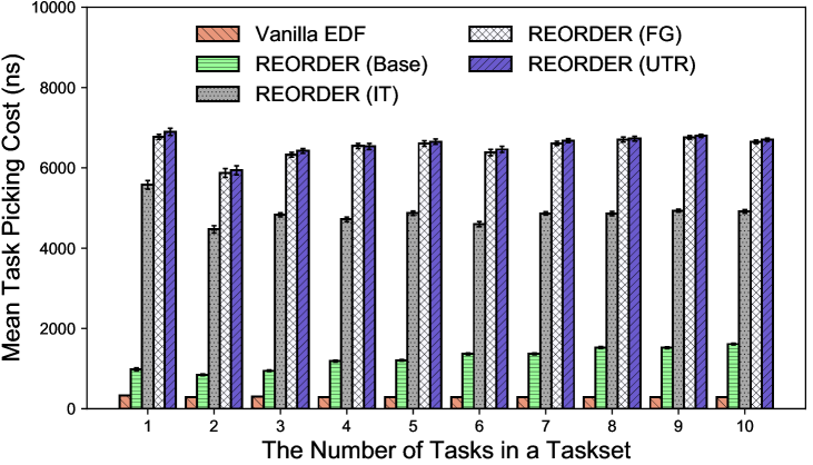
Fig. 5: The execution time cost (in nanoseconds) for the scheduling functions of the vanilla EDF and the randomized EDF. The vanilla EDF bar represents the mean execution times processed by the function $\mathtt{pick\_next\_dl\_entity()}$ while the other three EDF bars present the mean execution times for $\mathtt{pick\_rad\_next\_dl\_entity()}$ that carries out the randomization algorithm.

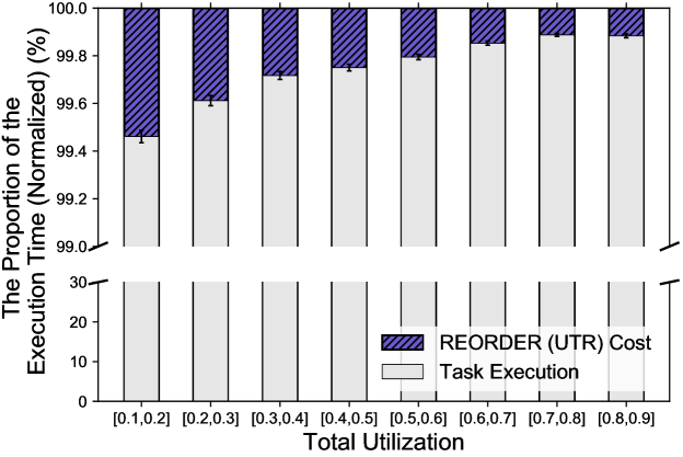
Fig. 6: The proportion of the cost of the REORDER protocol to the task execution times in the fine-grained switching with idle time randomization scheme. The randomization protocol overhead is provably inversely proportional to the taskset’s total utilization. The upper part of the figure is scaled to $99\%-100\%$ for better readability.

Next we examine the proportion of the scheduling overhead to the task’s execution. We do this by comparing the cumulative time cost of the randomization protocol with the cumulative task execution times during the $5$ second test duration for each taskset. Here, we consider the fine-grained switching with idle time randomization and unused time reclamation scheme (REORDER (UTR)) as it has the largest overhead among all possible schemes. Fig. 6 shows the mean proportion of the cost of the REORDER (UTR) protocol to the task execution times with varying total utilization. The results indicate that the overhead of the REORDER protocol is inversely proportional to the taskset’s total utilization. Since a taskset with higher utilization spends more of its time executing actual RT jobs, it dilutes the influence from the overhead. The utilization group $[0.8,0.9]$ has an average of $0.12\%$ overhead while it is $0.54\%$ for the $[0.1,0.2]$ utilization group. Considering there is typically an overestimation in the range $5\%$ and $15\%$ for task WCET calculations [45], the overhead of the REORDER protocol is negligible for most RTS.

VII Discussion

Although we only focused on the fact that REORDER can reduce the predictability of conventional dynamic priority scheduler, this idea improves the security posture of future RTS in a more fundamental way. For any scheduling policy, one can infer the amount of information leaked from the system. This information, for instance, will be useful for the engineers to analyze the potential vulnerability (associated with timing inference attacks) of the given system.

Consider a schedule $\mathcal{S}$ that is output from the randomization protocol (referred to as ground-truth process) and let $\mathcal{S}^{\prime}$ be the attackers (potentially semi-correct) observation about the schedule (noted as observation). We can define the information leakage as the amount of uncertainty (of the adversary) as follows: the uncertainty about the ground-truth process minus the attackers uncertainty (about the true schedule) after receiving the (fuzzy) observation (i.e., the amount of the reduction of uncertainty due to receiving the observation). One can then use mutual information [46, Ch. 2] (e.g., $\underset{\tilde{u}}{\sup}\leavevmode\nobreak\ I(\mathcal{S};\mathcal{S}^{\prime})$ where $\tilde{u}$ is the possible decoding strategies that an adversary can use and $I(\mathcal{S};\mathcal{S}^{\prime})=H(\mathcal{S})-H(\mathcal{S}|\mathcal{S}^{\prime})$ is the mutual information) between the ground-truth and the observation as a measure of leakage. A high dependency between the ground-truth and the observation leads to a high information leakage. This implies that the adversary can have a good estimation of the ground-truth. The frameworks developed in this work aims to increase the randomness of the output of the scheduler and reduce the dependency between $\mathcal{S}$ and the $\mathcal{S}^{\prime}$. This is because, for the randomized scheduler, there are more true schedules that are consistent with a given observation. We highlight that defining the exact relationship between the produced randomness and the leakage of the system will require further study. We intend to explore this aspect in future work.

While REORDER reduces the chances of the success of timing inference attacks (and hence improves the security), it is not free from trade-offs. For instance, as we observe in Fig. 5 and 6, the randomization logic adds extra overheads to the scheduler. In this work we did not attempt to derive any analytic upper-bound on the number of context switches and leave this for future work.

Note that it may be possible that some (heavily utilized) tasksets can not be randomized and in that case both EDF and REORDER output the same schedule. For instance, let us consider the taskset $\Gamma_{ex3}=\{\tau_{1},\tau_{2},\tau_{3},\tau_{4}\}$ with the following parameters: $C_{1}=1,C_{2}=3,C_{3}=2,C_{4}=4$ and $T_{1}=5,T_{2}=8,T_{3}=9,T_{4}=20$ (with $T_{i}=D_{i},1\leq i\leq 4$). The taskset is schedulable by EDF since $\sum\limits_{1\leq i\leq 4}\frac{C_{i}}{T_{i}}=0.997<1$. However, in this case the budgets (e.g., WCIB) are always negative for all the tasks, e.g., $V_{1}=-2,V_{2}=-1,V_{3}=-4,V_{4}=-4$. Therefore, at each scheduling point all the low-priority jobs will be excluded from priority inversion and only the shortest deadline job will be selected – i.e., the same schedule as EDF.

VIII Related Work

Krüger et al. [23] proposed a combined online/offline randomization scheme to reduce determinisms for time-triggered (TT) systems where tasks are executed based on a pre-computed, offline, slot-based schedule. The scheduling paradigms for TT systems are different than dynamic priority RTS. The closest line of work is TaskShuffler [24] where authors proposed to randomize task schedules for fixed-priority (e.g., RM) systems. However the methods developed in both of the above are not directly applicable for dynamic priority systems. Unlike fixed priority systems, obfuscating schedules for EDF scheduling is not straightforward due to run-time changes to task priorities. Besides, as we describe in Appendix -B, the calculation of schedule entropy in prior work does not correctly capture the randomness for all scenarios. Prior work also assumes all the jobs of the tasks always execute with WCET and hence may not be practical for real applications.

Zimmer et al. [47] propose the mechanisms to detect the execution of unauthorized instructions that leverages the information obtained by static timing analysis. An architectural approach that aims to create hardware/software mechanisms to detect anomalies is studied by Yoon et al. [15]. Threats to covert timing channels for RTS has been addressed in prior research for fixed-priority systems [39]. A scheduler-level modification is proposed in literature [48] that alters thread blocks (that may leak information) to the idle thread – the aim is to avoid the exploitation of timing channels while achieving real-time guarantees. The authors also developed locking protocols for preventing covert channels [49].

Issues regarding information leakage through storage timing channels (e.g., caches) in RTS, with different security levels, has been studied [8, 9] and further generalized [50]. The authors proposed a modification to the fixed-priority scheduling algorithm and introduced a state cleanup mechanism to mitigate information leakage through shared resources. However, this leakage prevention comes at a cost of reduced schedulability and is focused on fixed-priority systems. Besides, they may not be completely effective against timing inference attacks that focus on deterministic scheduling behaviors. REORDER works to break this inherent predictability of real-time scheduling by introducing randomness.

Bao et al.[51] model the behavior of the attacker and introduce a scheduling algorithm for a system with aperiodic tasks that have soft deadlines. They provide a trade-off between side-channel information leakage and the number of deadline misses. To the best of our knowledge REORDER is the first work that focuses on obfuscating schedule timing information for dynamic priority RTS with hard deadlines.

IX Conclusion

Malicious attacks on systems with safety-critical real-time requirements could be catastrophic since the attackers can destabilize the system by inferring the critical task execution patterns. In this work we focus on a widely used optimal real-time scheduling policy and make progress towards developing a solution for timing side-channel attacks. By using the approaches developed in this work (along with our open-source Linux kernel implementation) engineers of the systems can now have enough flexibility, as part of their design, to secure such safety-critical systems. While our initial findings are promising, we believe this is only a start towards developing a unified secure real-time framework in general.

-A Calculation of an Upper Bound of the Response Time

Under EDF, the response time calculation involves computing the busy-period of a task’s instance with deadline less than or equal to that instance [36]. Real-time theory uses the notion of interference, e.g., the amount of time a ready job of $\tau_{i}$ is blocked due to the execution of other higher priority jobs. To calculate the WCIB of a task, we measure the worst-case interference from its higher priority jobs. Note that with arbitrary priority inversions, any job could be delayed because of chain reactions, i.e., some low priority jobs in $lp(\tau_{i})$, delay the higher priority jobs (e.g., $\tau_{j},\forall d_{j}<d_{i}$), that in turn delay $\tau_{i}$ – hence $\tau_{i}$ may need more than its WCRT as calculated by the response time analysis [53, 35]. This phenomenon is known as back-to-back hit [53] and can be addressed by considering an extra instance of higher priority jobs. Therefore, without any assumptions on the execution patterns of $lp(\tau_{i})$, for a given release time $t=a$ we can calculate the upper bound of interference [35, 36, 53] experienced by $\tau_{i}$ as follows:

$$I_{i}(a)=\sum_{j\neq i,D_{j}\leq a+D_{i}}\min\left\{\left\lceil\tfrac{D_{i}}{T_{j}}\right\rceil+1,1+\left\lfloor\tfrac{a+D_{i}-D_{j}}{T_{j}}\right\rfloor+1\right\}C_{j}.$$ (3)

Note that the extra execution times (e.g., $+1$ in Eq. (3)) are added in the interference calculation to prevent the effects of back-to-back hit from higher priority jobs. For a given release time $a$, the response time of $\tau_{i}$ [35, 36] (relative to $a$) is given by: $R_{i}(a)=\max\left\{C_{i},W_{i}(a)-a\right\}$ where $W_{i}(a)$ denotes the workload of $\tau_{i}$ and calculated by $W_{i}(a)=\left(\left\lfloor\frac{a}{T_{i}}\right\rfloor+1\right)C_{i}+I_{i}(a)$. Finally we can compute the upper bound of WCRT of $\tau_{i}$ as follows: $R_{i}=\max\left\{R_{i}(a)\right\},\leavevmode\nobreak\ 0\leq a<\widehat{R}-C_{i}$ where $\widehat{R}$ is calculated by an iterative fixed point search, that is $\widehat{R}=r^{(k+1)}=r^{(k)}$ for some iteration $k$ where $r^{(\cdot)}$ is the upper bound of any busy-period length. We can calculate this upper bound using the following recurrence relation: $r^{(0)}=\sum\limits_{\tau_{i}\in\Gamma}C_{i},\leavevmode\nobreak\ r^{(k+1)}=\sum\limits_{\tau_{i}\in\Gamma}\left\lceil\frac{r^{(k)}}{T_{i}}\right\rceil C_{i}$. This sequence $r^{(k)}$ converges to $\widehat{R}$ in a finite number of steps if we assume that the taskset is schedulable (i.e., $\sum\limits_{\tau_{i}\in\Gamma}\frac{C_{i}}{T_{i}}\leq 1$) [36].

-B Limitations of Existing Entropy Calculation Approach

In order to evaluate the performance of a randomized scheduler, we need to have a measure of the randomness of the output of the scheduler. For a taskset with hyperperiod of length $L$, define the $L$ dimensional random vector $\mathcal{S}^{k}=\left[S_{1}^{k},\cdots,S_{L}^{k}\right]$ representing the schedule of hyperperiod $k$, where the random variable $S_{t}^{k}\in\{\tau_{0},...,\tau_{n}\}$ denotes the task (including the idle task) scheduled at the $t$-th slot of hyperperiod $k$. Note that the random vectors $\mathcal{S}^{k}$ for different values of $k$ are independent and identically distributed (i.i.d.) random variables. Therefore the average randomness of the whole output is equal to the randomness in a single hyperperiod.

In the past [24], researchers defined the entropy of the schedule $\mathcal{S}^{k}$ using Shannon entropy [46, Ch. 2] as a measure of the randomness, i.e., $H(\mathcal{S}^{k})=-\sum\limits_{s_{1}^{k}\in\{\tau_{0},\cdots,\tau_{n}\}}\cdots\sum\limits_{s_{L}^{k}\in\{\tau_{0},\cdots,\tau_{n}\}}\mathbb{P}(\mathcal{S}^{k}=[s_{1},\cdots,s_{L}])\times\log_{2}\mathbb{P}(\mathcal{S}^{k}=[s_{1}^{k},\cdots,s_{L}^{k}])$ with the assumption that $0\times\log_{2}0=0$. There are two major issues in calculating the schedule entropy using the above method.

First, in order to obtain $H(\mathcal{S}^{k})$, we need to calculate the distribution $\mathbb{P}({\mathcal{S}^{k}})$ – calculating this distribution has exponential complexity and is not computationally tractable in practice. Also, estimating this distribution requires a very high number of samples. To address this problem, we proposed [24] to use the sum of the entropy of random variables $S_{t}^{k}$, $t\in\{1,..,L\}$ as the measure of randomness (referred to as upper-approximated schedule entropy): $\widetilde{H}(\mathcal{S}^{k})=\sum_{t=1}^{L}H(S_{t}^{k}),$ where $H(S_{t}^{k})=-\sum\limits_{s_{t}^{k}\in\{\tau_{0},\cdots,\tau_{n}\}}\mathbb{P}(S_{t}^{k}=s_{t}^{k})\log_{2}\mathbb{P}(S_{t}^{k}=s_{t}^{k})$. Note that for $\pi=0$, choosing $m=1$ gives us $\widehat{H}(\mathcal{S}^{k},m,\pi,K)=\widetilde{H}(\mathcal{S}^{k})$ and choosing $m=L$ outputs $\widehat{H}(\mathcal{S}^{k},m,\pi,K)\rightarrow{H}(\mathcal{S}^{k})$, as $K\rightarrow\infty$. The main limitations of upper approximated schedule entropy $\widetilde{H}(\mathcal{S}^{k})$ is that it completely ignores the regularities that exist in $\mathcal{S}^{k}$ due to the dependencies among random variables. For instance, suppose a taskset contains two tasks: $\Gamma=\{\tau_{1},\tau_{2}\}$ and a schedule for first $5$ slots in $2$ individual hyperperiods is as follows: $\mathcal{S}_{1}\in\{(\tau_{1},\tau_{2},\tau_{1},\tau_{2},\tau_{1}),(\tau_{2},\tau_{1},\tau_{2},\tau_{1},\tau_{2})\}$, assuming each vector with equal probability. Let us consider another schedule $\mathcal{S}_{2}$ that has all possible $2^{5}$ vectors of $\tau_{1}$ and $\tau_{2}$ of length $5$ with equal probability. Then $\widetilde{H}(\mathcal{S}_{1})=\widetilde{H}(\mathcal{S}_{2})$ even though the randomness of $\mathcal{S}_{2}$ is much higher (i.e., $H(\mathcal{S}_{1})=1$ while $H(\mathcal{S}_{2})=5$). Therefore, $\widetilde{H}(\mathcal{S}^{k})$ cannot capture the randomness correctly.

Second, consider an instance where many of the schedules produced in different hyperperiods have very similar patterns in the first few slots and different patterns in the latter slots (or vice versa). In such cases $H(\mathcal{S}^{k})$ cannot capture the similarities and considers the observed hyperperiods as distinct ones – this leads us to search for dissimilarities in intervals smaller than the whole length of the hyperperiod. In what follows we propose an entropy measure to capture the randomness of a schedule using the concept of limited size intervals that resolves both the aforementioned issues and provides a better way to quantitatively compute randomness.

-C Comparison With True and Approximate Entropy

Recall that obtaining the true entropy (e.g., $H(\cdot)$) is not feasible in practice since it has an asymptotic complexity. Therefore, we compare approximate entropy (e.g., $\widehat{H}(\cdot)$ with $H(\cdot)$ by measuring the correlation observed from small tasksets. We generate tasksets that have $[3,5]$ tasks with $T_{i}\in\{2,4,5,10,20\}$ where the task utilizations and WCET are generated using methods from Section IV-C1. Each taskset has a common hyperperiod $L=20$ (allowing us to evaluate enough schedules for a reasonable time). For each taskset we observe the schedule for $K=1500$ hyperperiods and estimate the true entropy. Given a fixed taskset, generating unique schedules (e.g., $K\rightarrow\infty$) leads to actual entropy $H(\cdot)$ since more tasks appear at each slot. For approximate entropy $\widehat{H}(\cdot)$ we set interval length $m=\lceil 0.35L\rceil$ and dissimilarity threshold $\pi=0.1L$ by trial-and-error and measure the correlation.

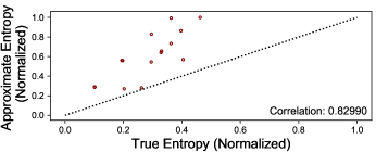
Fig. 7: The correlation between true and approximate entropy (the values are normalized to $[0,1]$).

The true and approximate entropy do not depend on the length of the hyperperiod – instead, the approximation error (as can be seen from Fig. 7) is due to the assumption of independence between intervals. While we observe that the correlation between true and approximate entropy is relatively high (e.g., $\approx\!\!0.82$) the approximated schedule entropy, $\widehat{H}(\cdot)$ should be used to compare the relative randomness of two schedules (that is also the focus of our evaluation).

-D REORDER Variables in Real-time Linux Implementation

The implementation of the REORDER protocol on the Linux kernel modifies four files:

• include/linux/sched.h (task/job-specific variables introduced in Section V-D1).

• kernel/sched/sched.h (scheduler-specific variables, as presented below).

• kernel/sched/core.c (scheduling functions that govern all schedulers in the kernel).

• kernel/sched/deadline.c (scheduling functions for $\mathtt{SCHED\_DEADLINE}$ – the main REORDER algorithms were implemented here).

Besides the task-specific variables introduced in Section V-D1, there are scheduler-specific variables declared and used in our implementation, as shown in the listing below.

⬇

struct dl_rq {

....

/* scheduler specific parameters */

struct hrtimer reorder_pi_timer; // schedule timer

u64 reorder_pi_timer_start_time; // timer start

bool reorder_idle_time_acting; // idle status

// scheme (Base, IT, FT, UTR)

enum reorder_scheduling_mode reorder_mode;

....

};

The variable $\mathtt{reorder\_mode}$ is used to determine the randomization scheme to be used in the scheduler. The enumeration for the scheme options are defined in the same source file (kernel/sched/sched.h) and shown in the following listing.

⬇

enum reorder_scheduling_mode {

REORDER_NORMAL, // task only randomization

REORDER_IDLE_TIME, // + idle time scheduling

REORDER_FINE_GRAINED,// + fine-grained switching

REORDER_RECLAMATION // + unused time reclamation

};

References

- [1] R. Wilhelm, J. Engblom, A. Ermedahl, N. Holsti, S. Thesing, D. Whalley, G. Bernat, C. Ferdinand, R. Heckmann, T. Mitra, F. Mueller, I. Puaut, P. Puschner, J. Staschulat, and P. Stenström, “The worst-case execution-time problem—overview of methods and survey of tools,” ACM TECS, vol. 7, no. 3, pp. 36:1–36:53, 2008.
- [2] C.-Y. Chen, S. Mohan, R. B. Bobba, R. Pellizzoni, and N. Kiyavash, “How to precisely whack that mole: Predicting task executions in real-time systems using a novel (scheduler) side-channel,” 2018. [Online]. Available: https://arxiv.org/abs/1806.01814
- [3] C.-Y. Chen, A. Ghassami, S. Nagy, M.-K. Yoon, S. Mohan, N. Kiyavash, R. B. Bobba, and R. Pellizzoni, “Schedule-based side-channel attack in fixed-priority real-time systems,” Tech. Rep., 2015.
- [4] J. Westling, “Future of the Internet of things in mission critical applications,” 2016.
- [5] N. Falliere, L. O. Murchu, and E. Chien, “W32. Stuxnet dossier,” White paper, Symantec Corp., Security Response, vol. 5, p. 6, 2011.
- [6] R. M. Lee, M. J. Assante, and T. Conway, “Analysis of the cyber attack on the ukrainian power grid,” SANS Industrial Control Systems, 2016.
- [7] M.-K. Yoon, S. Mohan, J. Choi, J.-E. Kim, and L. Sha, “SecureCore: A multicore-based intrusion detection architecture for real-time embedded systems,” in IEEE RTAS, 2013, pp. 21–32.
- [8] S. Mohan, M.-K. Yoon, R. Pellizzoni, and R. B. Bobba, “Real-time systems security through scheduler constraints,” in IEEE ECRTS, 2014, pp. 129–140.
- [9] R. Pellizzoni, N. Paryab, M.-K. Yoon, S. Bak, S. Mohan, and R. B. Bobba, “A generalized model for preventing information leakage in hard real-time systems,” in IEEE RTAS, 2015, pp. 271–282.
- [10] M. Hasan, S. Mohan, R. B. Bobba, and R. Pellizzoni, “Exploring opportunistic execution for integrating security into legacy hard real-time systems,” in IEEE RTSS, 2016, pp. 123–134.
- [11] K. Jiang, L. Batina, P. Eles, and Z. Peng, “Robustness analysis of real-time scheduling against differential power analysis attacks,” in IEEE ISVLSI, 2014, pp. 450–455.
- [12] J. Son and J. Alves-Foss, “Covert timing channel analysis of rate monotonic real-time scheduling algorithm in MLS systems,” in IEEE Inf. Ass. Wkshp, 2006, pp. 361–368.
- [13] D. Agrawal, B. Archambeault, J. R. Rao, and P. Rohatgi, “The em side—channel (s),” in International Workshop on Cryptographic Hardware and Embedded Systems. Springer, 2002, pp. 29–45.
- [14] H. Bar-El, H. Choukri, D. Naccache, M. Tunstall, and C. Whelan, “The sorcerer’s apprentice guide to fault attacks,” Proc. of the IEEE, vol. 94, no. 2, pp. 370–382, 2006.
- [15] S. Mohan, S. Bak, E. Betti, H. Yun, L. Sha, and M. Caccamo, “S3A: Secure system simplex architecture for enhanced security and robustness of cyber-physical systems,” in ACM HiCoNS, 2013, pp. 65–74.
- [16] T. Xie and X. Qin, “Improving security for periodic tasks in embedded systems through scheduling,” ACM TECS, vol. 6, no. 3, p. 20, 2007.
- [17] M. Lin, L. Xu, L. T. Yang, X. Qin, N. Zheng, Z. Wu, and M. Qiu, “Static security optimization for real-time systems,” IEEE Trans. on Indust. Info., vol. 5, no. 1, pp. 22–37, 2009.
- [18] M. M. Z. Zadeh, M. Salem, N. Kumar, G. Cutulenco, and S. Fischmeister, “SiPTA: Signal processing for trace-based anomaly detection,” in ACM EMSOFT, 2014.
- [19] C. L. Liu and J. W. Layland, “Scheduling algorithms for multiprogramming in a hard-real-time environment,” JACM, vol. 20, no. 1, pp. 46–61, 1973.
- [20] “Erika Enterprise,” http://erika.tuxfamily.org/drupal.
- [21] “Real-time executive for multiprocessor systems (RTEMS),” https://www.rtems.org.
- [22] D. Faggioli, F. Checconi, M. Trimarchi, and C. Scordino, “An EDF scheduling class for the Linux kernel,” in Real-Time Linux Wkshp, 2009.
- [23] K. Krüger, M. Völp, and G. Fohler, “Vulnerability analysis and mitigation of directed timing inference based attacks on time-triggered systems,” in EUROMICRO ECRTS, vol. 106, 2018, pp. 22:1–22:17.
- [24] M.-K. Yoon, S. Mohan, C.-Y. Chen, and L. Sha, “TaskShuffler: A schedule randomization protocol for obfuscation against timing inference attacks in real-time systems,” in IEEE RTAS, 2016, pp. 1–12.
- [25] “Implementation of REORDER on Linux with RT Patch,” https://github.com/rt-reorder/RT-Linux-REORDER.git.
- [26] M. R. Guthaus, J. S. Ringenberg, D. Ernst, T. M. Austin, T. Mudge, and R. B. Brown, “Mibench: A free, commercially representative embedded benchmark suite,” in IEEE WWC-4, 2001, pp. 3–14.
- [27] A. K. Mok, “Fundamental design problems of distributed systems for the hard-real-time environment,” Massachusetts Institute of Technology, Tech. Rep., 1983.
- [28] S. K. Baruah, A. K. Mok, and L. E. Rosier, “Preemptively scheduling hard-real-time sporadic tasks on one processor,” in IEEE RTSS, 1990, pp. 182–190.
- [29] J. Y.-T. Leung and M. Merrill, “A note on preemptive scheduling of periodic, real-time tasks,” Inf. proc. letters, vol. 11, no. 3, pp. 115–118, 1980.
- [30] D. Isovic, Handling sporadic tasks in real-time systems: combined offline and online approach. Mälardalen University, 2001.
- [31] J. Kelsey, B. Schneier, D. Wagner, and C. Hall, “Side channel cryptanalysis of product ciphers,” in Euro. Symp. on Res. in Comp. Sec., 1998, pp. 97–110.
- [32] D. Page, “Theoretical use of cache memory as a cryptanalytic side-channel.” IACR Crypt. ePrint Archive, vol. 2002, p. 169, 2002.
- [33] D. A. Osvik, A. Shamir, and E. Tromer, “Cache attacks and countermeasures: the case of aes,” in Crypt. Track at the RSA Conf., 2006, pp. 1–20.
- [34] S. K. Baruah, “Resource sharing in EDF-scheduled systems: A closer look,” in IEEE RTSS, 2006, pp. 379–387.
- [35] L. George, N. Rivierre, and M. Spuri, “Preemptive and non-preemptive real-time uniprocessor scheduling,” INRIA, https://hal.inria.fr/inria-00073732/file/RR-2966.pdf, Tech. Rep., 1996, [Online].
- [36] M. Spuri, “Analysis of deadline scheduled real-time systems,” INRIA, https://hal.inria.fr/inria-00073920/file/RR-2772.pdf, Tech. Rep., 1996, [Online].
- [37] S. M. Pincus, “Approximate entropy as a measure of system complexity.” Proc. of the Nat. Ac. of Sc., vol. 88, no. 6, pp. 2297–2301, 1991.
- [38] R. W. Hamming, “Error detecting and error correcting codes,” Bell Labs Tech. Journal, vol. 29, no. 2, pp. 147–160, 1950.
- [39] J. Son and J. Alves-Foss, “Covert timing channel analysis of rate monotonic real-time scheduling algorithm in MLS systems,” in IEEE Inf. Ass. Wkshp, 2006, pp. 361–368.
- [40] A. Gujarati, F. Cerqueira, and B. B. Brandenburg, “Schedulability analysis of the Linux push and pull scheduler with arbitrary processor affinities,” in IEEE ECRTS, 2013, pp. 69–79.
- [41] M. Bertogna and S. Baruah, “Limited preemption EDF scheduling of sporadic task systems,” IEEE Trans. on Ind. Info., vol. 6, no. 4, pp. 579–591, 2010.
- [42] E. Bini and G. C. Buttazzo, “Measuring the performance of schedulability tests,” RTS Journal, vol. 30, no. 1-2, pp. 129–154, 2005.
- [43] “Real-Time Linux (RTL) Collaborative Project,” https://wiki.linuxfoundation.org/realtime/.
- [44] V. M. Weaver, “Linux perf_event features and overhead,” in FastPath, vol. 13, 2013.
- [45] R. Wilhelm, J. Engblom, A. Ermedahl, N. Holsti, S. Thesing, D. Whalley, G. Bernat, C. Ferdinand, R. Heckmann, T. Mitra, F. Mueller, I. Puaut, P. Puschner, J. Staschulat, and P. Stenström, “The worst-case execution-time problem - overview of methods and survey of tools,” ACM Trans. Embed. Comput. Syst., vol. 7, no. 3, pp. 36:1–36:53, May 2008.
- [46] T. M. Cover and J. A. Thomas, Elements of information theory, 2012.
- [47] C. Zimmer, B. Bhat, F. Mueller, and S. Mohan, “Time-based intrusion detection in cyber-physical systems,” in ACM/IEEE ICCPS, 2010, pp. 109–118.
- [48] M. Völp, C.-J. Hamann, and H. Härtig, “Avoiding timing channels in fixed-priority schedulers,” in ACM ASIACCS, 2008, pp. 44–55.
- [49] M. Völp, B. Engel, C. J. Hamann, and H. Härtig, “On confidentiality-preserving real-time locking protocols,” in IEEE RTAS, 2013, pp. 153–162.
- [50] S. Mohan, M.-K. Yoon, R. Pellizzoni, and R. B. Bobba, “Integrating security constraints into fixed priority real-time schedulers,” RTS Journal, vol. 52, no. 5, pp. 644–674, 2016.
- [51] C. Bao and A. Srivastava, “A secure algorithm for task scheduling against side-channel attacks,” in ACM TrustED, 2014, pp. 3–12.
- [52] J. P. Lehoczky, “Fixed priority scheduling of periodic task sets with arbitrary deadlines,” in IEEE RTSS, 1990, pp. 201–209.
- [53] N. Audsley, A. Burns, M. Richardson, K. Tindell, and A. J. Wellings, “Applying new scheduling theory to static priority pre-emptive scheduling,” SE Journal, vol. 8, no. 5, pp. 284–292, 1993.