Passive Static Equilibrium with Frictional Contacts and Application to Grasp Stability Analysis

Abstract

This paper studies the problem of passive grasp stability under an external disturbance, that is, the ability of a grasp to resist a disturbance through passive responses at the contacts. To obtain physically consistent results, such a model must account for friction phenomena at each contact; the difficulty is that friction forces depend in non-linear fashion on contact behavior (stick or slip). We develop the first polynomial-time algorithm which either solves such complex equilibrium constraints for two-dimensional grasps, or otherwise concludes that no solution exists. To achieve this, we show that the number of possible “slip states” (where each contact is labeled as either sticking or slipping) that must be considered is polynomial (in fact quadratic) in the number of contacts, and not exponential as previously thought. Our algorithm captures passive response behaviors at each contact, while accounting for constraints on friction forces such as the maximum dissipation principle.

I INTRODUCTION

Stability analysis in the presence of frictional contacts is one of the foundational problems of multi-fingered robotic manipulation. In particular, a key characteristic of a grasp is the ability to resist given disturbances, formulated as wrenches externally applied to the grasped object. This is equivalent to determining the stability of a multi-body system under applied loads, a problem that is pervasive in grasp analysis but also encountered in other scenarios, including simulation of general rigid bodies with frictional contacts.

We believe that an important distinction to make in such analysis is between active and passive stability. Consider for example the grasp shown in Fig. 1. Will the grasp resist each of the two disturbances $\bm{w}_{1},\bm{w}_{2}$ applied to the object? Clearly, in each case, there exists a combination of contact forces that obey friction laws (are inside their respective friction cones) and sum up to counterbalance the disturbance ($\bm{c}_{1}$ together with $\bm{c_{3}}$ in the case of $\bm{w}_{1}$, and $\bm{c_{2}}$ in the case of $\bm{w}_{2}$). However, intuition tells us that $\bm{c}_{1}$ and $\bm{c_{3}}$ can only arise if contacts 1 and 3 have been preloaded with enough normal force to sustain the needed level of friction. In the absence of such a preload, or if the magnitude of the disturbance is too large relative to the preload, the object will just slip out. In contrast, $\bm{c}_{2}$ arises passively, strictly in response to the disturbance, and matching it in magnitude, thus $\bm{w}_{2}$ is always resisted.

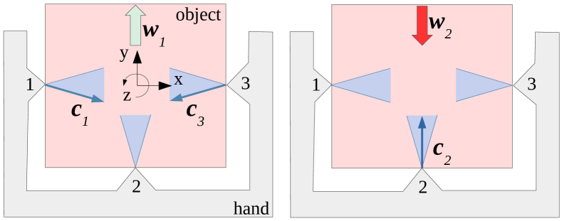
Figure 1: A grasping scenario where a hand establishes multiple frictional contacts (numbered 1-3) with a target object. External disturbance $\bm{w}_{1}$ (left, pushing the object up) can be resisted by contact forces $\bm{c}_{1}$ and $\bm{c}_{3}$, but only if contacts 1 and 3 have been actively pre-loaded with enough normal force to generate the corresponding friction forces. In contrast, disturbance $\bm{w}_{2}$ (right, pushing the object down), regardless of its magnitude, will always be passively resisted by contact force $\bm{c}_{2}$.

To account for these differences, we believe that a grasp stability model should be able to answer the following query, which we refer to as passive grasp stability. We assume that we are given the geometry of the grasp (i.e. the shape of the hand and object, and thus the contact locations) as well as the contact preloads actively applied by the motors (if any). A known external wrench is then applied to the object. Our query is formulated as: Based only on passive effects (arising naturally in response to the disturbance), will the system find a way to rebalance contact forces allowing it to remain in static equilibrium, or will the application of the disturbance lead to movement? We seek a model that provides global guarantees: if no solution to the equilibrium problem is found, we should be able to guarantee that none exists for the given instance.

Despite significant efforts (which we review in the next section), no existing grasp model achieves all these goals. Numerous studies do not consider contact preload when assessing grasp stability, or do not make the distinction between active and passive effects. Other approaches use simplified models for determining contact responses to external forces and fail to account for constraints arising from the dissipation of energy through friction. Finally, previous work searches for equilibrium configurations using iterative algorithms that run the risk of getting stuck in local optima, and thus cannot make strong global guarantees about the absence of a solution.

In this paper, we introduce a grasp stability model that accounts for all these constraints, and, in the two-dimensional case, allows for an efficient (polynomial time) algorithm to answer the passive stability query. We use more realistic friction constraints, where frictional forces are not linearly related to the externally applied wrench, and obey the maximum dissipation principle. Our main contributions are as follows:

• For two-dimensional grasps, we show that the total number of possible “slip states” for the system (where each contact is labeled as sticking or slipping, and the direction of slip is also determined) that must be considered under rigid body constraints is polynomial — in fact, quadratic — in the number of contacts.

• We use this result to derive the first polynomial-time algorithm that can provably determine if a solution exists to the passive equilibrium problem for a multi-contact grasp under an externally applied wrench, using friction constraints that obey the maximum dissipation principle.

The ability to make strong guarantees about the existence of equilibrium is one of the most attractive features of analytical models as compared to data-driven approaches. Previous methods either sacrifice this ability (e.g. by introducing iterative algorithms that are not guaranteed to converge), or simplify the constraints such that results can be physically inconsistent. We attempt to avoid such a trade off here, while preserving the ability to solve the equilibrium query efficiently.

II RELATED WORK

One class of trivially stable robotic grasps consists of form-closure grasps, which completely immobilize the grasped object. As the object is completely kinematically constrained, it will be stable in the face of arbitrary applied wrenches - even in the absence of friction. Checking if a grasp has form closure can be done by solving a linear program [9]. However, form closure grasps require a large number of contacts (at least 7 in the three dimensional case [15],[10]) and are not generally achievable with most robotic hands. Hence, grasps that do not exhibit form closure are of primary interest to this investigation. As was described in the Introduction, the existence of a solution to the equilibrium equations alone is not a sufficient condition for stability. Neglecting the mechanisms by which contact wrenches arise leads to false positives in cases where solutions exist, but do not arise in practice.

For a given robotic grasp, Pang et al. [12] group applied external wrenches into three classes:

• Weakly Stable Loads: a solution to the equilibrium equations exists for given friction coefficients at the contacts. This can be tested for by solving a linear program.

• Strongly Stable Loads: A subset of Weakly Stable Loads, the applied load leads to zero workpiece acceleration for given friction coefficients. This is equivalent to non-positive virtual work for every virtual motion that satisfies the kinematic constraints of the grasp.

• Frictionless Stable Loads: A small subset of the Strongly Stable Loads. Pang et al. show that if a load is weakly or strongly stable in the frictionless case, it is also strongly stable for all positive friction coefficients. Membership can be tested for by solving a linear program.

An algorithm very commonly used in practice to determine the total space of possible resultant wrenches as long as each individual contact force obeys (linearized) friction constraints was introduced by Ferrari and Canny [6]. They call this space the Grasp Wrench Space (GWS), which can also be used to test a grasp for force closure. This geometric method is an example of an algorithm we can use to determine the weakly stable loads as described above. It is an example of a method for stability analysis that does not account for the distinction between active and passive wrench reaction and the necessity of a preload in a grasp to withstand certain applied wrenches. In general - when trying to determine the stability of a grasp - an enumeration of the first class of applied loads is of limited use due to the possibility of false positives.

The final class of loads as defined by Pang and summarized above is overly conservative, as friction is a powerful tool to achieve stable grasps. The grasp in Fig. 1 for example is unstable in the frictionless case. The second class of loads is most useful for grasp stability analysis. Given a load known to be in the first class, in order to test for membership in the second we need to develop an algorithm that tests if the physically correct solution (i.e. the one that would arise in reality) lies in the space of solutions to the equilibrium equations; we need to develop further constraints that discriminate if a solution to the equilibrium equations is physically correct.

One approach to this problem is to resolve the statical indeterminacy by introduction of compliance. This reduces the solution space to at most a single solution, which is deemed to be the physically correct one. Of course, the physical correctness depends on the correctness of the assumptions made in resolving the statical indeterminacy. In his works [1][2][3] Bicchi assumes a linear compliance matrix (see also [4]), which is also a potential limitation, as it assumes a linear stiffness of the contacts. Friction forces, however, are non linear with respect to the relative sliding motion at the contacts.

Prattichizzo et al. [14] built on the previous work by Bicchi and developed tools for grasp force optimization that specifically take into account the kinematics of the hand. They also improve on the linear friction model used by Bicchi in order to alleviate some limitations of the linear model we will discuss in the next section. The complexity of their algorithm is exponential in the number if contacts and may hence be infeasible to deploy. Furthermore, its stability prediction is somewhat conservative, as we will show later in this paper.

III Passive Equilibrium Formulation

This section introduces the general framework of our problem. Consider a grasp that consist of $m$ contacts. Each contact is defined by a location on the surface of the object and a normal direction (determined by the local geometry of the bodies in contact). For any contact-specific vector (such as contact force or relative contact motion), we will use subscript $n$ to denote the component lying in the normal, and subscript $t$ to denote the component lying in the tangent direction.

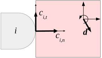
Figure 2: Notation used the paper. At contact $i$, $c_{i,n}$ denotes the magnitude of the normal component of the contact force while $c_{i,t}$ denotes its tangential component. These are expressed in the contact reference frame, chosen such that one of axes aligns with the normal component, and the other axis with the tangential component. $\bm{d}$ denotes virtual object motion expressed in the object coordinate frame.

We use the vector $\bm{c}\in\mathbb{R}^{2m}$ to denote contact forces, where $\bm{c}_{i}\in\mathbb{R}^{2}$ is the force at the i-th contact. Using the notation above, $c_{i,n}\in\mathbb{R}$ is the normal component of this force, and $\bm{c}_{i,t}\in\mathbb{R}$ is its tangential component, created via friction. We represent both as scalars, noting that we can always choose a convenient contact coordinate frame such that the normal direction lines up with one of the axes. Our notation is illustrated in Fig. 2. We now assume that the object is being disturbed by an externally applied wrench $\bm{w}\in\mathbb{R}^{3}$. The first, and simplest, condition necessary for equilibrium is the existence of a vector of contact forces that satisfies equilibrium constraints and hence balances the externally applied wrench. Furthermore, contact forces have to satisfy unilaterality (only positive normal forces) and friction constraints. At each contact $i$, the magnitude of the friction force has to be less than or equal to the normal force scaled by the friction coefficient $\mu$:

$$\bm{G}\bm{c} =\bm{w}$$ (1)

$$\bm{S}_{n}\bm{c} \geq 0$$ (2)

$$-\mu c_{i,n}\leq c_{i,t} \leq\mu c_{i,n} i=1,...,m$$ (3)

where $\bm{G}\in\mathbb{R}^{3\times 2m}$ is the grasp map matrix and $\bm{S}_{n}\in\mathbb{R}^{m\times 2m}$ is a selection matrix which selects only the normal components from the contact wrench vector. (In three dimensions, constraint (3) becomes non-linear, but is still convex.)

This problem is, in general, statically indeterminate; if a solution exists, there are infinitely many solutions. More importantly, the existence of a solution does not necessarily mean that the grasp is in equilibrium under the given wrench. In the simple example of Fig. 1 with the upwards disturbance (shown on the left) contact forces always exist that will satisfy (1)-(3), but, if the contacts have not been preloaded, these forces will not arise strictly in response to the disturbance. In other words, we are not yet capturing the passive response of the system to the disturbance. In order to capture the passive reaction of a grasp and resolve the indeterminacy, we start from the idea of using grasp compliance [4]. The key idea is to add constitutive equations that remove the indeterminacies. In particular, this is done by introducing virtual object movement and virtual springs at the contacts. Contact forces arise through virtual object motion loading the virtual springs. If there are springs for each component of the contact forces, the system becomes statically determinate: we can compute the linear stiffness of the grasp with respect to externally applied wrenches and hence contact forces that balance the disturbance. For now, we will neglect the compliance of the hand mechanism and will only concern ourselves with the stiffness of the contacts.

We begin by introducing virtual springs at the contacts, but, unlike previous work [1][2][3][14], these springs only affect forces in the normal direction. The deformation of those springs due to a virtual object motion $\bm{d}\in\mathbb{R}^{3}$ determines the normal forces at the contacts, supplying us with constitutive equations for those forces. We introduce matrix $\bm{K}$, a stiffness matrix for the virtual springs along the contact normals.

$$\bm{S}_{n}\bm{c}=\bm{K}\bm{S}_{n}\bm{G}^{T}\bm{d}$$ (4)

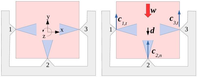
Figure 3: Linear relationship between friction and virtual object motion. Left: undisturbed system with 0 contact forces. Right: reaction to disturbance $\bm{w}$. Downward virtual motion $\bm{d}$ loads the normal component of $\bm{c}_{2}$ and resists the disturbance, but also creates frictional components at contacts 1 and 3. Since $\bm{c}_{1}$ and $\bm{c}_{3}$ now violate friction constraints, we could erroneously conclude that the disturbance can not be resisted.

Friction forces require additional consideration. In previous work [2], these were also included in a linear relationship such as (4). However, this approach has a major limitation: if such a linear relationship causes friction forces to leave the friction cone, we could erroneously conclude that the grasp is unstable. This is the case depicted in Fig. 3: using a linear friction constraint would lead us to conclude that equilibrium is not possible, where it is clear that stable equilibrium for this combination of grasp and applied wrench does indeed exist.

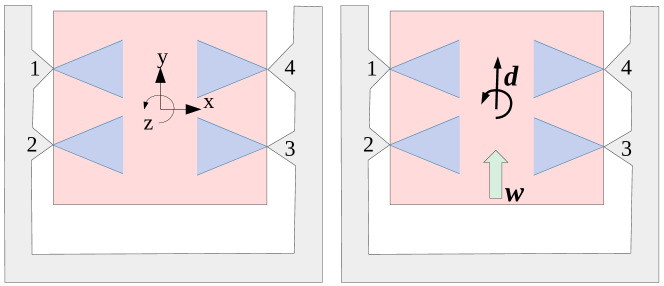
Figure 4: Unconstrained friction forces (except for friction cone constraint). Left: undisturbed system with 0 contact forces (also showing object reference frame). Right: reaction to disturbance $\bm{w}$. A virtual motion that is a combination of translation and rotation as shown can load the contacts enough to resist an arbitrary wrench, even in the absence of any preloads.

However, leaving friction forces constrained only by the friction cones described by (3) also leads to results that are physically inconsistent. Consider the case depicted in Fig. 4. Here, the existence problem (are there contact forces such that constraints (1)-(4) are satisfied) always has a solution, irrespective of the magnitude of the applied wrench, or the contact preload. The solution consists of a virtual object rotation that “loads” the contacts, creating the normal forces (and thus the friction) needed to resist the disturbance. However, in the absence of any initial preload, we would expect system to be unstable in the presence of the shown wrench, and the object to slide out. The underlying reason for this behavior is that we have not yet accounted for energy constraints on our system. According to the Maximum Dissipation Principle [13], at a contact that is slipping (virtual motion in the tangential direction is not zero) frictional force should dissipate as much energy as possible. This is achieved if friction opposes virtual motion, and lies on the edge of its friction cone. Thus, at a contact $i$ that slips (and thus has relative tangential motion), the friction force can be expressed as the vector of relative motion multiplied by an unknown scalar $\sigma_{i}$, and constrained to lie on the edge of the friction cone:

$$c_{i,t} = \sigma_{i}(\bm{G}^{T}\bm{d})_{i,t}$$ (5)

$$\sigma_{i} \leq 0$$ (6)

$$\left|c_{i,t}\right| = \mu c_{i,n}$$

$$\text{for all}~{}i~{}\text{s.t.}~{}(\bm{G}^{T}\bm{d})_{i,t}\neq 0$$

For a contact that does not slip, the friction force is still only bound by (3). We now also have a constitutive relation for frictional forces, and hence all the constraints we require to model a grasp. However, the formulation we have arrived at does not allow for an efficient solution method: we have to distinguish between the possible slip states of a contact in order to decide which constraints apply. With $m$ contacts, considering only two (stick/slip) possible states for each contact still leaves us with a total of $2^{m}$ possible combinations for our system.

In this light, our contributions are as follows. For two-dimensional grasps, we will show that, given rigid body movement constraints, the number of possible slip states for the system is in fact polynomial in the number of contacts, even if also including the direction (positive or negative) of slip along a tangential axis. Then, we will show how this result allows us to break the problem down into a polynomial number of sub-problems, which can be solved efficiently.

IV Number of Possible Slip States

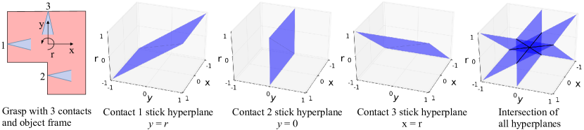
Figure 5: Arrangement of planes equivalent to contact stick-slip constraints. For the grasp shown on the left, each contact defines a plane in the three-dimensional space of possible object motions $\bm{d}=[x,y,r]$. For example, Contact 1 sticks if the translation component of $\bm{d}$ along $y$ is counteracted by an equal rotational component $r$. Similarly, Contact 2 sticks if the $y$ component of $\bm{d}$ is 0, and so on.

We focus here on the problem of determining the state of each contact for a two-dimensional grasp with $m$ contacts. In its simplest form, this state only considers two possibilities per contact: sticking or slipping. However, we consider three possible states for each contact: stick, plus slip in the positive or negative direction of the local tangent axis. We define a slip state $S_{k}\in\{-1,0,1\}^{m}$ as a vector comprising information about slip at every contact. The $i$-th element of $S_{k}$, labeled $s_{i}^{k}$, defines the state of contact $i$ in state $k$ as follows:

$$s_{i}^{k}=0 : \text{stick},(\bm{G}^{T}\bm{d})_{i,t}=0$$ (8)

$$s_{i}^{k}=-1 : \text{negative slip},(\bm{G}^{T}\bm{d})_{i,t}<0$$ (9)

$$s_{i}^{k}=1 : \text{positive slip},(\bm{G}^{T}\bm{d})_{i,t}>0$$ (10)

Finally $\mathbb{S}$ is the set of all possible system slip states, thus $S_{k}\in\mathbb{S}$ for $k=1..\#(\mathbb{S})$, where $\#(\mathbb{S})$ is the cardinality of $\mathbb{S}$. At first glance, $\#(\mathbb{S})=3^{m}$: since each contact can have three states, the total number of states for the system is exponential in the number of contacts. Indeed, this is the approach used in previous studies that account for stick/slip at each contact [14]. Our main insight is that not all of these possible state combinations are consistent with rigid body movement of the grasped object. Assuming that the object is rigid, displacement at each contact reference frame must be related to object displacement at all other contacts, and a linear function of object displacement $\bm{d}$ expressed at the object reference frame. In fact, we will show that, when accounting for rigid body motion, $\#(\mathbb{S})$ is quadratic in $m$.

IV-A Slip states as plane arrangements

We make an argument from geometry to show that not all combinations of slip states are indeed possible. First, let us look at the stick condition defined above: in the three-dimensional space of possible object motions $\bm{d}=[x,y,r]$, the constraint $(\bm{G}^{T}\bm{d})_{i,t}=0$ defines a plane. Note that this plane goes through the origin. Any object motion lying on this plane will result in zero relative tangential motion at this contact. Motion in the halfspace where $(\bm{G}^{T}\bm{d})_{i,t}\geq 0$ will result in slip along the tangential axis in the positive direction, while motion in the complementary halfspace $(\bm{G}^{T}\bm{d})_{i,t}\leq 0$ will result in slip in the negative direction. Combining the planes defined by each contact, we obtain the possible states for all of our contacts. These planes segment the space of object motions into:

• 3-dimensional “regions” where all contacts are slipping;

• 2-dimensional “facets” (region boundaries on a single plane) where one contact is sticking;

• 1-dimensional “lines” (intersections of multiple planes) where multiple contacts are sticking.

By construction, since all of our planes go through the origin, the only possible zero-dimensional “point” intersection is the origin itself (see Fig. 5.) Given this partition of the space of possible object motions, it follows that any system slip state $S_{k}$ that is consistent with a possible object motion must correspond to either a region, a face, or a line created by this plane arrangement. Finding the maximum number of three-dimensional regions given $m$ planes is equivalent to finding the maximum number of regions on a sphere cut with $m$ great circles, which is known to be $O(m^{2})$ [8]. However, the regions do not define all the combinations of slip states we care about. We must also consider the cases where at least one contact sticks, namely the “facets” and “lines” defined as above.

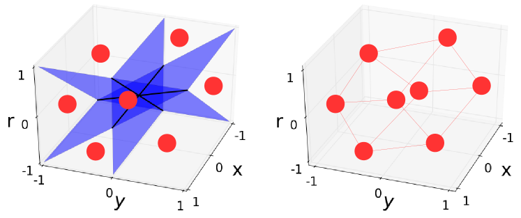
Figure 6: Dual polyhedron for the arrangement of planes. Each region of the arrangement of planes (red dot) corresponds to a vertex of the polyhedron (for clarity, only 7 regions are marked in the left figure). Vertices are connected if the corresponding regions share a facet.

We can show that the number of regions, facets and lines is bounded polynomially by applying Zaslavski’s formula [7]. Let $f_{k}^{(d)}(n)$ be the number of “k-faces” of an arrangement of $n$ hyperplanes in $d$ dimensional space, where $k$ is the dimension of the face. Then, the following holds:

$$f_{k}^{(d)}(n)\leq{n\choose d-k}\sum_{i=0}^{k}{n-d+k\choose i}$$ (11)

In our case, the total number of slip states we are interested in is equal to $\sum_{k=0}^{3}f_{k}^{(3)}(m)$ and hence polynomial in $m$. This is, however, an upper bound that will not be attained in our case, as we show next. Let us construct the dual convex polyhedron to our arrangement of planes, which will be instrumental in enumerating all possible slip states. Each region of the plane arrangement corresponds to a vertex of the polyhedron, and each two dimensional boundary (facet) between regions corresponds to an edge (vertices corresponding to neighboring regions are connected, see Fig. 6.) We can ensure this polyhedron is convex by selecting, as the representative vertex for each region, a point where the region intersects the unit sphere. We note that the lines of our plane arrangement correspond to faces of the dual polyhedron. The dual polyhedron thus fully describes our possible slip states.

Like any convex polyhedron, the dual we have constructed can be represented by a 3-connected planar graph. From this result, we can bound number of slip states even more closely, than with Zaslavski’s formula: Any maximal planar graph with $V$ vertices has at most $3V-6$ edges and $2V-4$ faces and hence the number of edges and faces of our polyhedron are linearly bounded by the number its vertices. Since we have shown the number of vertices to be $O(m^{2})$, so are the number of edges and faces. Thus, the number of slip states we must consider is quadratic in the number of contacts.

IV-B Slip state enumeration

We can now present a complete procedure for enumerating all possible slip states $S_{k}$ of an $m$-contact system that are consistent with rigid body object motion.

Step 1. We begin by enumerating all the slip states $S_{k}$ corresponding to regions in our plane arrangement. We achieve that using Algorithm 1. We note that for any state $S_{k}$ obtained by this algorithm, all contacts are slipping, in either the positive or negative direction ($s_{i}^{k}=\pm 1$ for all $i$, we have not yet considered sticking cases).

Algorithm 1

Initialize $\mathbb{S}$ with empty state $S$

for $i=1..m$ do

     for $k=1..\#(S)$ do

         Remove $S_{k}$ from $\mathbb{S}$

         if Region $S_{k}$ has component above plane $P_{i}$ then

              Create region $S_{k+}=\{S_{k},1\}$

              Add $S_{k+}$ to $\mathbb{S}$

         end if

         if Region $S_{k}$ has component below plane $P_{i}$ then

              Create region $S_{k-}=\{S_{k},-1\}$

              Add $S_{k-}$ to $\mathbb{S}$

         end if

     end for

end for

Step 2. Now we create the slip states corresponding to facets in the plane arrangements (one sticking contact). As mentioned before, these correspond to edges of the dual polyhedron, so we begin this step by constructing the dual polyhedron. We already have its vertices: each state $S$ created at the previous step defines a region of the plane arrangement, and thus corresponds to a vertex of the dual polyhedron. Then, for every two states $S_{k},S_{l}$ in $\mathbb{S}$ that differ by a single $s_{i}$, we add the edge between them to the dual polyhedron (note that thus our polyhedron is also a partial cube where edges connect any two vertices with Hamming distance equal to 1 [5]). Furthermore, we also create an additional state $S_{kl}$ corresponding to the facet between $S_{k}$ and $S_{l}$. This will be identical to both $S_{k}$ and $S_{l}$, with the difference that $s_{i}=0$ (the entry corresponding to the plane that this facet is on is set to 0).

Step 3. Finally, we must create the slip states corresponding to lines in our plane arrangement (multiple sticking contacts), which correspond to faces of the dual polyhedron. We obtain the faces of our dual polyhedron by computing the Minimum Cycle Basis (MCB) of the undirected graph defined by its edges (computed at the previous step). This gives us $F-1$ of the faces of our polyhedron; to see why consider that the number of cycles in the minimum cycle basis is given by $E-V+1$ [11]. Recall the Euler-Poincaré characteristic $\chi=V-E+F$ relating the number of vertices, edges and faces of a manifold. For a convex polyhedron $\chi=2$, and from this we can derive the number of faces of our dual polyhedron to be equal to $E-V+2$. The last face is obtained as the symmetric sum of all the cycles in the MCB (defined as in [11]).

Once we have the cycles corresponding to the faces of the dual polyhedron, we convert them into slip states as follows. For each cycle, starting from the slip state $S_{k}$ corresponding to any of the vertices in the cycle, we set $s_{i}=0$ for any plane $i$ that is traversed by an edge in the cycle. The total number of slip states $S$ we obtain is thus equal to the number of regions, facets and lines of the plane arrangement, which is the same as the number of vertices, edges and faces of its dual polyhedron. We have already shown that this is polynomial (quadratic) in the number of planes (contacts). We also show that the enumeration algorithm above has polynomial runtime.

We note that Step 1 has two nested loops, with one iterating over planes and the other one over existing states. The number of states at the end of this step is bounded by $m^{2}$, thus the running time of this Step is $O(m^{3})$. Step 2 must check every state against every other one, with $O(m^{2})$ states, thus its running time is $O(m^{4})$. Finally, the dominant part of Step 3 is the computation of the MCB. We have used an implementation with $O(E^{3}+VE^{2}\text{log}V)$ running time, where $V$ and $E$ are the number of vertices and edges of the dual polyhedron. Since both $E$ and $V$ are polynomial in $m$, the running time of the MCB algorithm is as well. Thus our complete enumeration method has polynomial runtime in the number of contacts $m$.

Algorithm 2

Build $\mathbb{S}$, the set of all possible slip states

for $k=1..\#(S)$ do

     Given $S_{k}$, solve system (1), (2), (4), (12-14)

     if solution found then

         Return: grasp stable

     end if

end for

Return: grasp unstable

V Complete Equilibrium Determination

In this section we use the set of slip states $\mathbb{S}$ previously derived to arrive at a complete algorithm for determining the existence of passive equilibrium for our system.

V-A Solution for a particular slip state

We recall that a slip state $S_{k}=\{s_{i}\},i\in\{1..m\}$, where $s_{i}^{k}=\{-1,0,1\}$. For each contact $i$, $s_{i}^{k}=-1$ means that the contact is slipping in the negative direction, $s_{i}^{k}=1$ means slip in the positive direction, and finally $s_{i}^{k}=0$ means the contact is sticking. Critically, the fact that $S_{k}$ comprises not just stick/slip information, but also the direction of slip, turns friction into a simple linear dependency on object motion. The complete friction constraints are:

$$c_{i,t}=\mu c_{i,n} ~{}~{}~{}\text{for all}~{}i~{}\text{s.t.}~{}s_{i}^{k}=-1$$ (12)

$$c_{i,t}=-\mu c_{i,n} ~{}~{}~{}\text{for all}~{}i~{}\text{s.t.}~{}s_{i}^{k}=1$$ (13)

$$-\mu c_{i,n}\leq c_{i,t}\leq\mu c_{i,n} ~{}~{}~{}\text{for all}~{}i~{}\text{s.t.}~{}s_{i}^{k}=0$$ (14)

Intuitively, these correspond to the following three states:

1. The contact slips in the negative tangential direction. Friction opposes the relative motion s.t. $c_{i,t}=\mu c_{i,n}$.

2. The contact slips in the positive tangential direction. Friction opposes the relative motion s.t. $c_{i,t}=-\mu c_{i,n}$.

3. The contact sticks (it exhibits no relative motion in the tangential direction). The friction force lies in the interior of the friction cone s.t. $-\mu c_{j,n}\leq c_{j,t}\leq\mu c_{jn}$.

Thus, for any given slip state $S_{k}$, the system given by Eqs. (1), (2), (4) and (12-14) is easy to solve. In fact, we notice that we have a total of $3+2m$ unknowns (vectors $\bm{d}$ and $\bm{c}$). From equilibrium in eq. (1), the normal force constitutive relations in eq. (4) and the above eq. (12&13) we have $3+m+(m-l)$ constraints, where $l$ is the number of slipping contacts. We can use the condition that the remaining $m-l$ stationary contacts do not exhibit any relative motion in the tangential direction to formulate $m-l$ additional constraints, leading to a total of $3+2m$ constraints matching the number of unknowns. For a given $S_{k}$ we can thus trivially find a solution to the linear system of equations given by Eqs. (1),(4) and (12&13). We then check if the solution also meets Eqs. (14) (friction cone at sticking contacts) and (2) (normal force non-negativity). If the matrix corresponding to Eqs. (1),(4) and (12&13) is singular this operation is replaced by a simple linear program, which looks for a solution in the nullspace satisfying also equations (14),(2). Only if the solution we obtain satisfies all constraints do we deem the grasp to be stable for slip state $S_{k}$.

V-B Complete equilibrium algorithm

We can now formalize our complete algorithm using the components outlined so far (Algorithm 2). We first build the total set of possible slip states $\mathbb{S}$. Then, for every $S_{k}\in\mathbb{S}$, we check for a solution to the system described above. If one exists, we deem the grasp stable. If, after enumerating all possible $S_{k}$, we do not find one that admits a solution, we deem the grasp unstable. We make two important observations regarding Algorithm 2. First, its running time is polynomial in the number $m$ of contacts. This follows trivially from the results obtained so far. We know that $\#(\mathbb{S})$ is polynomial in $m$, as is the process for building it. For each $S_{k}$, we then solve at most a linear program with $2m+3$ unknowns, which also has a polynomial runtime, which completes this result.

Second, Algorithm 2 guarantees that, if no solution is found, none exists that satisfies the constraints of our system. $\mathbb{S}$ provably contains all the slip states consistent with rigid body movement; for each of these, equilibrium conditions form a linear program for which we can provably find all solutions (if they exist). So, under the assumed formulation (virtual springs used to determine passive reaction, and frictional constraints including the maximum dissipation principle), if a solution exists to the equilibrium problem, we must find it.

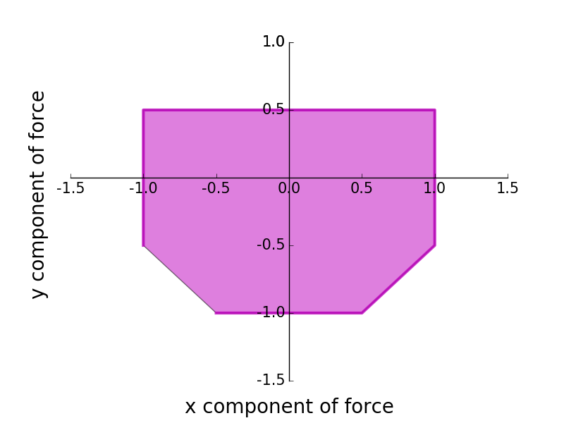
(a) Slice through the three dimensional GWS for zero applied torque

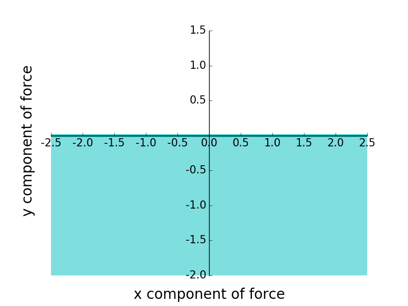
(b) Resistible forces with no preload (our algorithm)

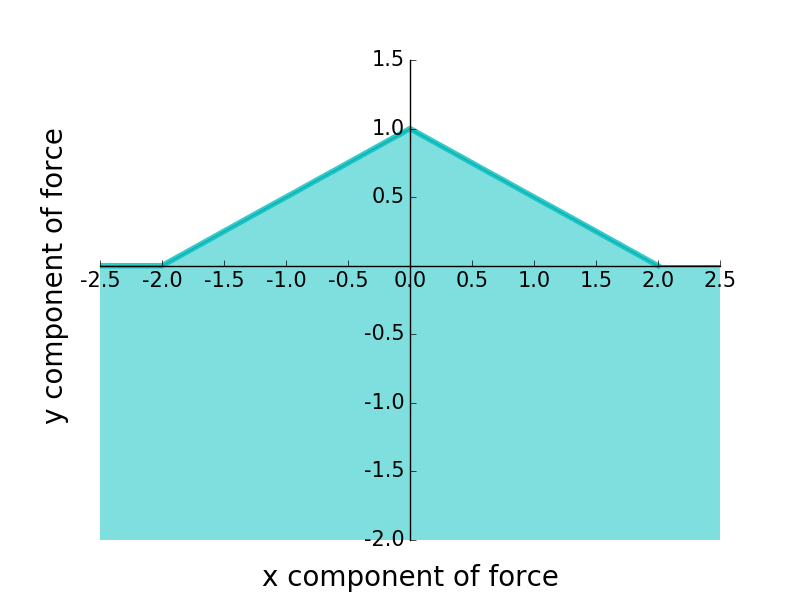
(c) Resistible forces with a preload such that the normal force at each conctact is 1 (our algorithm)

Figure 7: Grasp stability representations for the grasp in Fig. 1. The GWS representation (a) shows the space of applied wrenches the grasp can resist with contact forces that satisfy only friction constraints (shaded). We are using the L1 norm GWS, meaning the normal component of a contact force is at most equal to 1. Our algorithm (b)(c) captures passive resistance up to arbitrary reaction forces, as long as they arise passively in response to the disturbance. The space of resistible wrenches produced by our algorithm is thus bounded only on the upper edge of the space, as indicated by the line border. A boundary without this line indicates arbitrary resistance in the corresponding directions.

VI RESULTS

In this section we will demonstrate that our framework - in contrast to previous approaches to this problem - predicts the correct force distributions and makes an accurate prediction on grasp stability. We will utilize the grasp examples introduced in Figs. 1, 3 & 4, because the correct force distribution and stability of the grasp is easily understood intuitively.

Let us first consider the problem first described in the Introduction: can we discriminate which applied wrenches will be balanced purely passively, and where an active preload of the grasp is required? Recall that there exist contact forces in the interior of the friction cones that balance both wrenches shown in Fig. 1. Perhaps the most commonly used approach to grasp stability analysis is the Grasp Wrench Space method [6]. Indeed, when we consider the slice through the GWS visualized in Fig. 7(a) we can see that there exist contact forces that balance arbitrary forces in the plane. However, we argue that while $\bm{w}_{2}$ will always be reacted passively, no matter the preload, in order to react $\bm{w}_{1}$ we require the grasp to have been sufficiently preloaded. The GWS method correctly indicates the existence of equilibrium contact forces but does not predict if they may arise, and hence does not capture the necessity of a preload.

Now let us apply our framework to this problem: Using our algorithm, we can test the resistance of this grasp to forces in the plane. We do this by discretizing the direction of application of force to the object and finding the maximum resistible force in each direction using a binary search. Figs. 7(b) & 7(c) shows the region of resistible wrenches for a grasp without and with a preload respectively. As our algorithm takes into account passive effects it correctly predicts that, in both cases, forces with non-positive component in the y-axis and arbitrary magnitude can be withstood. Indeed, for any applied wrench $\bm{w}=(0,w_{y},0),w_{y}\leq 0$ our framework predicts contact forces $(0,0)$ at contacts 1 and 3, and contact force $(-w_{y},0)$ at contact 2 (see Table I). Furthermore, it captures the necessity of a preload in order to resist forces with positive component in the y-direction: For $w_{y}>0$ our algorithm finds no solution, and hence the grasp must be unstable to this disturbance, unless an appropriate preload is applied.

We have already shown the main deficiency of compliance based approaches such as in [1][2][3][14] (recall Fig. 3), which are commonly used to predict contact forces that arise in grasps due to disturbances. We can now use this grasp (Fig. 1) and our algorithm to show that the improvements to a linear compliance suggested by Prattichizzo et al. [14] lead to overly conservative stability estimates. Their approach allows each contact to be in one of three states: sticking, slipping or detached. A slipping contact may not apply any frictional forces, while a detached contact may not apply any force at all. If we try every possible combination of states and modify the compliance of the grasp accordingly, this alleviates some of the problems of the purely linear compliance approach: If we consider contacts 1 & 3 to be slipping, our grasp in Fig. 1 may now withstand arbitrary forces, where $w_{y}\leq 0$.

This approach, however, does not allow us to arrive at the correct result in cases where $w_{y}\geq 0$. Consider the preloaded grasp before the application of an external wrench (Table I.) The contact forces on both contacts 1 & 3 lie on the friction cone edge in order to balance the preload applied by contact 2. If we now apply an external wrench $\bm{w}=(0,1,0)$, there exists no combination of sticking, slipping and detached contacts (and corresponding modifications of the linear compliance) that results in legal contact forces. Our algorithm, however, predicts a stable grasp (Table I), showing how important friction is for grasp stability and why a correct treatment of friction is fundamental to stability analysis. Furthermore, we have arrived at this result in polynomial time — we did not have to consider exponentially many slip states, as in [14].

$\bm{w}$	$P$	Stable	$\bm{f}_{1}$	$\bm{f}_{2}$	$\bm{f}_{3}$	$\bm{d}$
$(0,0,0)$	0	Yes	$(0,0)$	$(0,0)$	$(0,0)$	$(0,0,0)$
$(0,0,0)$	1	Yes	$(1,-0.5)$	$(1,0)$	$(1,0.5)$	$(0,0,0)$
$(0,-1,0)$	0	Yes	$(0,0)$	$(1,0)$	$(0,0)$	$(0,-1,0)$
$(0,-2,0)$	0	Yes	$(0,0)$	$(2,0)$	$(0,0)$	$(0,-2,0)$
$(0,1,0)$	0	No	-	-	-	-
$(0,1,0)$	1	Yes	$(1,-0.5)$	$(0,0)$	$(1,0.5)$	$(0,1,0)$
$(0,1.1,0)$	1	No	-	-	-	-

TABLE I: Contact forces $\bm{f}_{i}=(f_{n,i},f_{t,i})$ and virtual object motion $\bm{d}=(x,y,r)$ for the grasp in Fig. 1 and a range of applied wrenches $\bm{w}=(w_{x},w_{y},w_{z})$. The preload $P$ is such that the normal force at each contact is equal to either 0 or 1 before any wrench is applied. The object motion and applied wrenches are expressed in the coordinate frame shown in Fig. 1 and contact forces are expressed in frames as shown in Fig. 2.

$m$	2	3	4	5	6	7	8	9
$\#(\mathbb{S})$	10	26	50	82	122	170	226	290
$time(s)$	0.006	0.02	0.09	0.42	1.5	4.8	13.8	35.7

TABLE II: Number of slip states $\#(\mathbb{S})$ and computation time for grasps with $m$ randomly generated contacts.

$\bm{w}$	$P$	Stable	$\bm{f}_{1}$	$\bm{f}_{2}$	$\bm{f}_{3}$	$\bm{f}_{4}$	$\bm{d}$
$(0,0,0)$	$0$	Yes	$(0,0)$	$(0,0)$	$(0,0)$	$(0,0)$	$(0,0,0)$
$(0,0,0)$	$1$	Yes	$(1,0)$	$(1,0)$	$(1,0)$	$(1,0)$	$(0,0,0)$
$(0,2,0)$	$0$	No	-	-	-	-	-
$(0,-2,0)$	$0$	No	-	-	-	-	-
$(0,2,0)$	$1$	Yes	$(1,-0.5)$	$(1,-0.5)$	$(1,0.5)$	$(1,0.5)$	$(0,0,0)$
$(0,-2,0)$	$1$	Yes	$(1,0.5)$	$(1,0.5)$	$(1,-0.5)$	$(1,-0.5)$	$(0,0,0)$
$(0,0,3)$	$0$	Yes	$(1,0.5)$	$(0,0)$	$(1,0.5)$	$(0,0)$	$(0,-1,1)$
$(0,0,-3)$	$0$	Yes	$(0,0)$	$(1,-0.5)$	$(0,0)$	$(1,-0.5)$	$(0,1,-1)$
$(0,0,3)$	$1$	Yes	$(1.25,0.625)$	$(0.75,0.375)$	$(1.25,0.625)$	$(0.75,0.375)$	$(0,-0.25,0.25)$
$(0,0,-3)$	$1$	Yes	$(0.75,-0.375)$	$(1.25,-0.625)$	$(0.75,-0.375)$	$(1.25,-0.625)$	$(0,0.0.25,-0.25)$

TABLE III: Contact forces $\bm{f}_{i}=(f_{n,i},f_{t,i})$ and virtual object motion $\bm{d}=(x,y,r)$ for the grasp in Fig. 4 and a range of applied wrenches $\bm{w}=(w_{x},w_{y},w_{z})$ and preloads $P$. The object motion and applied wrenches are expressed in the coordinate frame shown in Fig. 4 and contact forces are expressed in frames as shown in Fig. 2.

Let us now look at the grasp in Fig. 4, with which we investigated the deficiency of solely constraining the friction forces to lie within the friction cones. These constraints would allow a solver to rotate the object; the normal forces built up this way allow for arbitrary friction forces and reaction of arbitrary wrenches. In contrast, our framework restricts the friction force as is physically correct, and negates equilibrium for any wrench $\bm{w}=(0,w_{y},0)$ if there is no preload (see Table III). Hence our algorithm correctly predicts that the contact forces required to balance this wrench will not arise passively.

Let us now apply a preload to the contacts such that the normal force at each contact is 1 (previous to the application of an external wrench). If we now apply $(0,w_{y},0)$ our algorithm predicts stability for $\|w_{y}\|\leq 4\mu$ only, where $\mu$ is the friction coefficient of the contacts (we have chosen $\mu=0.5$). Table III contains a summary of contact forces and virtual object motion for a range of different applied wrenches and preloads.

From a computational effort perspective, a summary of the performance of our algorithm for enumeration of slip states can be found in Table II. All computation was performed on a commodity computer with a 2.80GHz Inter Core i7 processor.

VII CONCLUSIONS

We have discussed the various pitfalls of physically accurate force distribution and grasp stability analysis that also provides strong guarantees. In order to solve this problem we considered contact slip states (where each contact is labeled as sticking or slipping, and the direction of slip is also determined) that are consistent with rigid body motion. The number of possible combinations of such states was shown to be quadratic in the number of contacts. Furthermore, we described a polynomial runtime algorithm to enumerate those slip states. We then showed the problem of force distribution for a two dimensional grasp to be efficiently solvable given the slip states of its contacts. Thus we broke the force distribution problem into a number of sub-problems, which we can efficiently solve. Recalling the above result that the number of these problems to be solved is quadratic in the number of contacts, we used this insight to develop an algorithm to investigate the distinction between active and passive reactions in grasping. This is a powerful tool for stability analysis, which in previous work required either approximation or the loss of global guarantees with respect to stability - our approach requires neither.

It is important to note that the problem of force distribution in general 3-dimensional space is much harder. Due to the non-convexity of the friction constraint derived from the maximum dissipation principle one cannot efficiently solve the problem even with prior knowledge of which contacts slip and which do not. While in two dimensions, two tangential axes will positively span the space of relative tangential motion (and there are hence 3 slip states per contact), in three dimensions there are infinitely many directions a contact can slip in. The enumeration of slip states in 3D grasping is nonetheless highly interesting and future work will focus on generalizing the algorithm presented in this paper to higher dimensions. Defining a high number of hyperplanes per contact could be a powerful tool in developing efficient algorithms that compute approximate solutions to the 3-dimensional grasping problem. In addition, we believe that our method of accounting for slip patterns through the geometry of hyperplane arrangements may be useful in improving the performance of quality metrics such as PCR and PGR, but also elsewhere in robotics.

References

- Bicchi [1993] Antonio Bicchi. Force distribution in multiple whole-limb manipulation. In Robotics and Automation, 1993. Proceedings., 1993 IEEE International Conference on, pages 196–201. IEEE, 1993.
- Bicchi [1994] Antonio Bicchi. On the problem of decomposing grasp and manipulation forces in multiple whole-limb manipulation. Robotics and Autonomous Systems, 13(2):127–147, 1994.
- Bicchi [1995] Antonio Bicchi. On the closure properties of robotic grasping. The International Journal of Robotics Research, 14(4):319–334, 1995.
- Cutkosky and Kao [1989] Mark R. Cutkosky and Imin Kao. Computing and controlling the compliance of a robotic hand. IEEE Transactions on Robotics and Automation, 5(2), 1989.
- Eppstein [2008] David Eppstein. Recognizing partial cubes in quadratic time. Journal of Graph Algorithms and Applications, 15(2), 2008.
- Ferrari and Canny [1992] C. Ferrari and J. Canny. Planning optimal grasps. In IEEE International Conference on Robotics and Automation, pages 2290–2295, 1992.
- Fukuda et al. [1991] Komei Fukuda, Shigemasa Saito, Akihisa Tamura, and Takeshi Tokuyama. Bounding the number of k-faces in arrangements of hyperplanes. Discrete Applied Mathematics, 31, 1991.
- Gleason et al. [1980] Andrew M. Gleason, L. M. Kelly, and R. E. Greenwood. Solutions: The twenty-fifth competition. The William Lowell Putnam mathematical competition : problems and solutions :1938-1964, 1980.
- Liu [1999] Yun-Hui Liu. Qualitative test and force optimization of 3-d form closure grasps using linear programming. IEEE Transactions on Robotics and Automation, 15(1), 1999.
- Markenscoff et al. [1990] Xanthippi Markenscoff, Luqun Ni, and Christos H. Papadimitriou. The geometry of grasping. The International Journal of Robotics Research, 9(1):61–74, 1990.
- Mehlhorn and Michail [2005] Kurt Mehlhorn and Dimitrios Michail. Implementing minimum cycle basis algorithms. In Sotiris E. Nikoletseas, editor, Experimental and Efficient Algorithms, pages 32–43. Springer Berlin Heidelberg, 2005.
- Pang and Trinkle [2000] J.-S. Pang and J. Trinkle. Stability characterizations of rigid body contact problems with coulomb friction. ZAMM - Journal of Applied Mathematics and Mechanics / Zeitschrift für Angewandte Mathematik und Mechanik, 80(10), 2000.
- Peshkin and Sanderson [1989] Michael A. Peshkin and Arthur C. Sanderson. Minimization of energy in quasi-static manipulation. IEEE Transactions on Robotics and Automation, 5(1), 1989.
- Prattichizzo et al. [1997] Domenico Prattichizzo, John Kenneth Salisbury, and Antonio Bicchi. Contact and grasp robustness measures: Analysis and experiments. In Experimental Robotics IV, pages 83–90. Springer Berlin Heidelberg, 1997.
- Somov [1900] P. Somov. über gebiete von schraubengeschwindigkeiten eines starren körpers bei verschiedener zahl von stützflächen. Zeitschrift für Mathematik und Physik, 45, 1900.