A General Framework for Bandit Problems Beyond Cumulative Objectives

Abstract

The stochastic multi-armed bandit (MAB) problem is a common model for sequential decision problems. In the standard setup, a decision maker has to choose at every instant between several competing arms, each of them provides a scalar random variable, referred to as a “reward.” Nearly all research on this topic considers the total cumulative reward as the criterion of interest. This work focuses on other natural objectives that cannot be cast as a sum over rewards, but rather more involved functions of the reward stream. Unlike the case of cumulative criteria, in the problems we study here the oracle policy, that knows the problem parameters a priori and is used to “center” the regret, is not trivial. We provide a systematic approach to such problems, and derive general conditions under which the oracle policy is sufficiently tractable to facilitate the design of optimism-based (upper confidence bound) learning policies. These conditions elucidate an interesting interplay between the arm reward distributions and the performance metric. Our main findings are illustrated for several commonly used objectives such as conditional value-at-risk, mean-variance trade-offs, Sharpe-ratio, and more.

Key words: Multi-armed bandit, risk, planning, reinforcement learning, upper confidence bound, optimism principle.

1 Introduction

Consider a sequential decision making problem where at each stage one of $K$ independent alternatives is to be selected. When choosing alternative $i$ at stage $t$ (also referred to as time $t$), the decision maker receives a reward $X_{{t}}$ that is distributed according to some unknown distribution $F^{\brk*{{i}}}$, $i=1,\ldots,K$ and is independent of $t$. (Where unambiguous, we avoid indexing $X_{t}$ with $i$, and leave that implicit; the information will be encoded in the policy that governs said choices, which will be detailed in what follows.) At time $t$, the decision maker has accumulated a vector of rewards $(X_{{1}},\ldots,X_{{t}})$. In our setting, performance criteria are defined by a function $\tilde{U}$ that maps the reward vector to a real-valued number. As $\tilde{U}(X_{1},\ldots,X_{t})$ is a random quantity, we consider the accepted notion of expected performance, i.e., $\mathbf{E}{\tilde{U}(X_{{1}},\ldots,X_{{t}})}$, assuming this expectation exists and is finite. An oracle, with full knowledge of the arms’ distributions, will make a sequence of selections based on this information so as to maximize the expected performance criterion. This serves as a benchmark for any other policy which does not have such information a priori, and hence needs to learn it on the fly. The gap between the former (performance of the oracle) and the latter (performance of the policy) represents the usual notion of regret in the learning problem.

The most ubiquitous performance criterion in the literature concerns the long run average reward, which involves the empirical mean, $\tilde{U}^{ave}(X_{{1}},\ldots,X_{{t}})=\frac{1}{t}\sum_{s=1}^{t}X_{{s}}$. In this case, the oracle rule, that maximizes the expected value of the above, just samples from the distribution with the highest mean value, namely, it selects $i^{*}\in\operatorname*{arg\,max}\{\int xdF^{\brk*{{i}}}(x)\}$. Learning algorithms for such problems date back to Robbins’ paper Robbins (1952) and were extensively studied subsequent to that. In particular, the seminal work of Lai and Robbins (1985) establishes that the normalized (per epoch) regret in this problem, when the arms are “well separated,” cannot be made smaller than $\mathcal{O}(\log T/T)$, and there exist learning algorithms that achieve this regret by maximizing a confidence bound modification of the empirical mean. (When the arms are not well separated, equivalent statements hold with order-$1/\sqrt{T}$.) Since then, this class of policies has come to be known as UCB, or upper confidence bound policies. Some strands of literature that have emerged from this include Auer et al. (2002) (non-asymptotic analysis of UCB-policies), Maillard et al. (2011) (empirical confidence bounds or KL-UCB), Agrawal and Goyal (2012) (Thompson sampling based algorithms), and various works which consider an adversarial formulation (see, e.g., Auer et al. (1995)).

Main research questions. In this paper we are interested in studying the above problem for more general path dependent objectives that are of interest beyond just the vanilla average. Many of these objectives bear an interpretation as “risk criteria” insofar as they focus on a finer probabilistic nature of the primitive distributions than the mean, and typically relate to the spread or tail behavior. Examples include: the so-called Sharpe ratio, which is the ratio between the mean and standard deviation; value-at-risk ($VaR_{\alpha}$) which focuses on the $\alpha$ percentile of the distribution (with $\alpha$ small); or a close counterpart that integrates (averages) the values out in the tail beyond that point known as the expected shortfall (or conditional value at risk; $CVaR_{\alpha}$). The last example is of further interest as it belongs to the class of coherent risk measures which has various attractive properties from the risk theory perspective. A discussion thereof is beyond the scope of this paper; cf. Artzner et al. (1999) for further details. In our problem setting, the above criteria are applied via the function $\tilde{U}$ to the empirical observations, and then the decision maker seeks, as before, to optimize its expected value. A typical example where such criteria may be of interest is that of clinical trials (one of the original motivations for the development of the MAB framework). More specifically, suppose several new drugs are sequentially tested on individuals who share similar characteristics. If we consider average performance, we may conclude that the best choice is a drug with a non-negligible fatality rate but a high success rate. If we wish to control the fatality rate then using $CVaR_{\alpha}$ for example may be appropriate.

While some of the above mentioned criteria have been examined in the decision making and learning literature (see references below), the analysis tends to be driven by specific properties of the criterion in question, and is very much done on a case-by-case basis. One of the purposes of this paper is to present a more unified approach to a large set of such problems. One of the main obstacles that arises under the non-cumulative criteria is the more complicated structure of the oracle rule. In particular, unlike the case of the mean objective, here the oracle rule need not select the same arm throughout the horizon of the problem. This presents further obstacles in identifying and characterizing a learning policy, as most such blueprints call for minimizing regret by mimicking the oracle rule. To that end, as our analysis will flesh out, under suitable conditions the oracle policy can be approximated (asymptotically) by a simple policy, that is, one that statically selects a single arm. This simplification can be leveraged to address the learning problem which becomes more tractable and amenable to optimism-based design principles. It is therefore of interest to understand and characterize in what instances does this simplified structure exist. This is one of the main thrusts of the paper.

Main contributions of this paper. In this paper we consider a general approach to the analysis of performance criteria where the oracle policy is a simple policy. We identify a class of criteria that we term Empirical Distribution Performance Measures (EDPM). In particular, let $\hat{F}$ be the empirical distribution of the vector $(X_{{1}},\ldots,X_{{t}})$, i.e., $\hat{F}(y)$ is the fraction of rewards less or equal to real valued $y$. An EDPM evaluates performance by means of a function ${U}$, which maps $\hat{F}$ to $\mathbb{R}$, i.e., ${U}(\hat{F})=\tilde{U}(X_{{1}},\ldots,X_{{t}})$. Alternatively, ${U}$ may also serve to evaluate the distributions of the random variables $X_{{s}}$ ($s=1,\ldots,t$). These evaluations may be aggregated to form a different type of performance criteria that we term “pseudo regret,” and consider as an intermediate learning goal. Our main results provide easily verifiable explicit conditions that characterize the asymptotic behavior of the oracle rule, and culminate in a $UCB$-type learning algorithm with either $\mathcal{O}(\log T/T)$ or $\mathcal{O}(1/\sqrt{T})$ normalized regret (depending on the properties of ${U}$ and the arm distributions).

While our framework encompasses many existing performance measures, there are some notable examples that are left out. One is the Maximum Drawdown, which measures the maximum decline from the highest historical peak in the reward sequence. This criterion cannot be expressed by our framework as it depends on the order of the reward sequence. Other criteria such as certain distortion risk measures and cumulative prospect theory can be expressed within our framework, however, they do not satisfy some of its requirements, hence our results are not directly applicable. Whether these could be incorporated into our framework remains open to future work. See further details in Section 6.

Previous works on bandits that concern path-dependent and risk criteria. Sequential performance measures of the type considered here were previously studied in Sani et al. (2012), which considered the Mean-Variance of the sequence and presented the MV-UCB, and MV-DSEE algorithms, and Vakili and Zhao (2016, 2015), which complete the regret analysis of said algorithms and also consider performance under Value at Risk. Zhu and Tan (2020) also consider the Mean-Variance and give a Thompson sampling-based method. Additionally, Agrawal and Devanur (2019) consider a constrained bandit problem with a concave objective. This may, for example, capture the Mean-Variance setting, however, it is not the main focus of the paper and the results are restricted to order $\mathcal{O}(\sqrt{T})$ regret (or order-$1/\sqrt{T}$ normalized regret in our setting).

Other works consider simpler performance measures that are more closely related to our notion of pseudo regret. Galichet et al. (2013) present the MaRaB algorithm which uses $CVaR_{\alpha}$ in its implementation, however, they analyze the average reward performance, and do so under the assumptions that $\alpha=0$, and the assumption that the $CVaR_{\alpha}$ and average optimal arms coincide. Tamkin et al. (2019) also consider $CVaR_{\alpha}$ and give a sample-wise optimistic algorithm. Bhat and Prashanth (2019) consider the concentration of risk measures and apply it exclusively to bound $CVaR_{\alpha}$ pseudo regret. It should be noted that some of their findings, and in particular the pseudo regret bound, where previously established in Cassel et al. (2018), which is an antecedent to the present paper. Zimin et al. (2014) consider criteria based on the mean and variance of distributions, and present and analyze the $\varphi-LCB$ algorithm. We note that these criteria correspond to a much narrower class of problems than the ones considered here. Maillard (2013) presents and analyzes the RA-UCB algorithm which considers the measure of entropic risk with a parameter $\lambda$.

Slightly farther afield, other works consider the best arm identification or simple regret settings. Kagrecha et al. (2019) propose distribution independent algorithms for a linear combination of the mean and $CVaR_{\alpha}$ measures. L.A. et al. (2020) consider the estimation of $CVaR_{\alpha}$ for both light and heavy tailed distributions, and provide an algorithm for best $CVaR_{\alpha}$ arm identification. Tran-Thanh and Yu (2014) consider a general functional of the arm distributions and demonstrate results on Mean-Variance, $VaR_{\alpha}$, and $CVaR_{\alpha}$ best arm and simple regret. Yu et al. (2017) consider a Mean-Variance best arm identification. David et al. (2018) consider a quantile risk constrained setting for best arm identification.

Finally, we mention two alternative settings that consider quantile-based sequential performance measures such as $VaR_{\alpha}$ and $CVaR_{\alpha}$. Torossian et al. (2019) consider the convergence of approximate dynamic programming in Markov Decision Processes (MDP), and Jiang and Powell (2018) consider a stochastic optimization setting with bandit feedback. The approach in our paper is quite distinct from these.

Organization. Throughout, all proofs are provided as a sketch that communicates their key ideas, with the full details deferred to the Appendix. In Section 2 we give initial motivation for our suggested class of performance criteria. In Section 3 we formulate the problem setting, oracle rule, and regret metric under non-cumulative criteria. In Section 4 we provide the main results, and in Section 5 we demonstrate them on well-known risk criteria. We also include some negative examples, which illustrate the implications of violation of the proposed conditions, indicating in some way the necessity of such conditions in achieving the unifying theme in our proposed framework.

2 A Motivating Example

In the standard bandit setting, for a sequence of integrable random variables we are interested in designing a policy $\pi$ that maximizes the average reward ${U}_{\pi}^{\text{ave}}=\mathbf{E}\delim{[}{]}1{\sum_{t=1}^{T}X_{{\pi},{t}}},$ or, equivalently, minimizes regret compared to an oracle strategy, which is known to pull a single arm throughout the horizon. It is well known that optimistic strategies achieve optimal performance in this setting. Now, suppose we seek to design a policy $\pi$ that maximizes ${U}_{\pi}^{CVaR_{\alpha}}=\mathbf{E}\delim{[}{]}1{\frac{1}{\delim\lceil\rceil*{t\alpha}}\sum_{s=1}^{\delim\lceil\rceil*{t\alpha}}X^{*}_{{\pi},{s}}},$ where $X^{*}_{{\pi},{s}}$ is the $s^{th}$ order statistic of $(X_{{\pi},{1}},\ldots,X_{{\pi},{t}})$. This is known as Conditional Value at Risk ($CVaR_{\alpha}$) or Expected Shortfall, at percentile level $\alpha\in(0,1)$, and is a widely accepted performance measure from the risk literature.

Question: Can we minimize regret using an optimistic strategy?

To answer this, we first need to understand what constitutes an optimistic strategy, which in turn requires that we further understand the oracle rule, which is aware of the true distributions of the arms. The current formulation of ${U}_{\pi}^{CVaR_{\alpha}}$ presents it as a direct function of the reward sequence. While this is very intuitive, it is in fact a sequence of mappings (one for each sample size) that do not naturally share a domain; studying this sequence can be challenging. In lieu of that, we first observe that ${U}_{\pi}^{CVaR_{\alpha}}$ may be reformulated in terms of a single function that evaluates the sequence of empirical reward distributions $\hat{F}_{t}^{\pi}$, where $\hat{F}_{t}^{\pi}(x)$ is the fraction of rewards less than or equal to $x$. Formally, ${U}_{\pi}^{CVaR_{\alpha}}=\mathbf{E}{{U}^{CVaR_{\alpha}}\brk 1{\hat{F}_{t}^{\pi}}}$ where

$${U}^{CVaR_{\alpha}}\brk 1{F}=\max_{z\in\mathbb{R}}z-\frac{1}{\alpha}\int_{-\infty}^{z}F(x)dx,$$

is the accepted notion for measuring $CVaR_{\alpha}$ for a random variable $X$ with cumulative distribution function $F$. In Appendix A we show that essentially any performance measure that is invariant to the order of the reward sequence may be reformulated as $\mathbf{E}{{U}\brk 1{\hat{F}_{t}^{\pi}}}$ for some function ${U}$. Importantly, this captures many well-known performance measures such as Mean-Variance, Entropic Risk, Sharpe Ratio, and more.

Having restricted ourselves to the class of performance measures that can be expressed this way, we have obtained a consistent way to evaluate performance, which is independent of the time $t$. Our study now turns to investigating the properties of the function ${U}$, in conjunction with the arm distributions, that allow for an optimistic strategy. In the case of $CVaR_{\alpha}$, if we only assume sub-Gaussian arm distributions, we find that ${U}^{CVaR_{\alpha}}$ may be non-smooth, and our framework can only guarantee a regret of $\mathcal{O}(1/\sqrt{T})$ using an optimistic strategy. However, if for example the arm distributions have positive density around their $\alpha$ percentile then we show that the same strategy only incurs $\mathcal{O}(\log T/T)$ regret. The remainder of this paper will flesh out these ideas and provide a set of easy to verify conditions that yield the results discussed in this section.

3 Problem Formulation

Model and admissible policies.

Consider a standard MAB with $\mathds{K}=\brk[c]*{1,\ldots,K},$ the set of arms. Arm $i\in\mathds{K}$ is associated with a sequence $X_{{i},{t}}$ ($t\geq 1$) of $i.i.d$ random variables with distribution $F^{\brk*{{i}}}\in\mathcal{D}$, the set of all distributions on the real line. When pulling arm $i$ for the $t^{th}$ time, the decision maker receives reward $X_{{i},{t}}$, which is independent of the remaining arms, i.e., the variables $X_{{i},{t}}$ (for all $i\in\mathds{K},t\geq 1$) are mutually independent.

We define the set of admissible policies (strategies) of the decision maker in the following way. Let $\tau_{i}\brk*{t}$ be the number of times arm $i$ was pulled up to time $t$. Let $V$ be a random variable over a probability space $\brk*{\mathbb{V},\mathcal{V},P_{v}}$ which is independent of the rewards. An admissible policy $\pi=\brk*{\pi_{1},\pi_{2},\ldots}$ is a random process recursively defined by

$$\pi_{t}:=\pi_{t}\brk*{V,\pi_{1},\ldots,\pi_{t-1},X_{{\pi},{1}},\ldots,X_{{\pi},{t-1}}}$$ (1)

$$\tau_{i}\brk*{t}=\sum_{s=1}^{t}\mathds{1}{\brk[c]*{\pi_{s}=i}}$$ (2)

$$X_{{\pi},{t}}:=X_{{i},{\tau_{i}\brk*{t}}}\text{, given the event }\brk[c]*{\pi_{t}=i}.$$ (3)

We denote the set of admissible policies by $\Pi$, and note that admissible policies $\pi$ are non anticipating, i.e., depend only on the past history of actions and observations, and allow for randomized strategies via their dependence on $V$. Formally, let $\brk[c]*{\mathcal{H}_{t}}_{t=0}^{\infty}$ be the filtration defined by $\mathcal{H}_{t}=\sigma\brk*{V,\pi_{1},X_{{\pi},{1}},\ldots,\pi_{t},X_{{\pi},{t}}}$, then $\pi_{t}$ is $\mathcal{H}_{t-1}$ measurable.

Empirical Distribution Performance Measures (EDPM).

The classical bandit optimization criterion centers on the empirical mean, i.e., $\frac{1}{t}\sum_{s=1}^{t}X_{{\pi},{s}}$. We generalize this by considering criteria that are based on the empirical distribution. Formally, the empirical distribution of a real number sequence $x_{1},\ldots,x_{t}$ is obtained through the mapping ${\hat{F}_{t}:\mathbb{R}^{t}\rightarrow\mathcal{D}}$, given by

$$\hat{F}_{t}\brk*{x_{1},\ldots,x_{t};\cdot}=\frac{1}{t}\sum_{s=1}^{t}\mathds{I}_{\brk[s]{x_{s},\infty}}(\cdot),$$ (4)

where $\mathds{I}_{\brk[s]{a,b}}(\cdot)$ is the indicator function of the interval $\brk[s]*{a,b}$ defined on the extended real line, i.e.

$$\mathds{I}_{\brk[s]{a,b}}\brk*{y}=\begin{cases}1\qquad,y\in[a,b]\\ 0\qquad,y\notin[a,b].\end{cases}$$

Of particular interest to this work are the empirical distributions of the reward sequence under policy $\pi$, and of arm $i$. We denote these respectively by,

$$\hat{F}_{t}^{\pi}(\cdot)~{}:=\hat{F}_{t}\brk*{X_{{\pi},{1}},\ldots,X_{{\pi},{t}};\cdot}$$ (5)

$$\hat{F}_{t}^{(i)}(\cdot):=\hat{F}_{t}\brk*{X_{{i},{1}},\ldots,X_{{i},{t}};\cdot}.$$ (6)

The decision maker possesses a function ${U}:\mathcal{D}\to\mathbb{R}$, which measures the “quality” of a distribution. The resulting criterion is called EDPM, and the decision maker aims to maximize $\mathbf{E}{{U}\brk 1{\hat{F}_{T}^{\pi}}}$. (Throughout it is assumed implicitly that the class of distributions and performance functions is such that this expectation exists and is finite valued.)

Oracle and regret.

For given horizon $T$, the oracle policy $\pi^{*}\brk*{T}=(\pi^{*}_{1}\brk*{T},\pi^{*}_{2}\brk*{T},\ldots)$ is one that achieves optimal performance given full knowledge of the arm distributions $F^{\brk*{{i}}}$ ($i\in\mathds{K}$). Formally, it satisfies

$$\pi^{*}\brk*{T}\in\operatorname*{arg\,max}_{\pi\in\Pi}\mathbf{E}\delim{[}{]}*{{U}\brk 1{\hat{F}_{T}^{\pi}}}.$$ (7)

Similar to the classic bandit setting, we define a notion of regret that compares the performance of policy $\pi$ to that of $\pi^{*}\brk*{T}$. The expected (normalized) regret of policy $\pi\in\Pi$ at time $T$ is given by,

$$R_{\pi}\brk*{T}:=\mathbf{E}\delim{[}{]}*{{U}\brk 1{\hat{F}_{T}^{\pi^{*}\brk*{T}}}-{U}\brk 1{\hat{F}_{T}^{\pi}}}.$$ (8)

We note that this definition is normalized with respect to the horizon $T$, thus transforming familiar regret bounds such as $\mathcal{O}(\log T)$ into $\mathcal{O}(\frac{\log T}{T})$. With that convention we simply refer to the above as the “regret” without added qualifiers.

Assumptions.

Beyond the existence and finiteness of expectations, flagged earlier, we make the following assumption throughout. Let the simplex in $\mathbb{R}^{K}$ be

$$\textstyle\Delta=\Big{\{}p=\brk*{p_{1},\ldots,p_{K}}\in\mathbb{R}^{K}\;\Big{|}\;\sum_{i=1}^{K}p_{i}=1,\;p_{i}\geq 0\;\forall i\in\mathds{K}\Big{\}},$$

and define the set of all convex combinations of the arms’ reward distributions by

$$\textstyle\mathcal{D}^{\Delta}=\Big{\{}F_{p}=\sum_{i=1}^{K}{p_{i}F^{\brk*{{i}}}}\;\Big{|}\;p\in\Delta\Big{\}}.$$ (9)

Let $i^{*}\in\operatorname*{arg\,max}{U}\brk 1{F^{\brk*{{i}}}}$ be an “optimal” arm. We assume that

$${U}\brk 1{F}\leq{U}\brk 1{F^{(i^{*})}}\quad,\forall F\in\mathcal{D}^{\Delta}.$$ (10)

While this assumption holds for many known performance measures, and seems crucial for obtaining the improved $\log T/T$ regret rate, we note that there is some loss of generality here. In Section 6, we give a few examples of known performance measures where 10 does not hold, and discuss how one could potentially address them within our framework. Finally, we note that 10 alone does not immediately imply that playing $i^{*}$ is optimal or even near-optimal over a finite horizon $T$ (for an illustration of this, see Section F.5).

4 Main Results

When defining an objective, it was sufficient to consider ${U}$ as a mapping from $\mathcal{D}$ (a set) to $\mathbb{R}$. Moving forward, our analysis relies on properties such as continuity and differentiability, which requires that we consider ${U}$ as a mapping between seminormed spaces. To that end $\mathcal{D}$ is a subset of an infinite dimensional vector space for which norm equivalence does not hold. This hints at the importance of using the “correct” (semi)norm for each ${U}$. As a result, our analysis is done with respect to a general seminorm $\norm{\cdot}$ and its matching seminormed space $L_{\norm{\cdot}}$. We therefore consider EDPMs as mappings ${U}:L_{\norm{\cdot}}\to\mathbb{R}$.

The goal of this work is to provide a generic analysis of the regret, similar to that of the classical bandit setting, and which culminates in the following result.

Theorem (Informal meta-result).

There exists an efficient algorithm such that:

1. Under suitable regularity conditions obtains regret $R_{\pi}\brk*{T}=\mathcal{O}(\frac{\log T}{\sqrt{T}});$

2. Under additional smoothness and gap conditions obtains regret $R_{\pi}\brk*{T}=\mathcal{O}(\frac{\log T}{{T}}).$

In what follows, we introduce the technical details required to make this statement rigorous. This culminates in Section 4.5, where Theorem 4 gives the desired statement, and where we also explain how the standard bandit setting fits into our framework. Unlike the classical bandit setting, the oracle policy $\pi^{*}\brk*{T}$, defined in 7, need not choose a single arm. Since the typical learning algorithms are structured to emulate the oracle rule, we need to first understand the structure of the oracle policy before we can analyze $R_{\pi}\brk*{T}$.

4.1 Insights From the Infinite Horizon Oracle

The oracle problem in 7 does not admit a tractable solution, in the absence of further structural assumptions. In this section we consider a relaxation of the oracle problem which examines asymptotic behavior. We provide conditions under which this behavior is “simple” thus suggesting it as a proxy for the finite time performance. More concretely, let ${U}_{\pi}=\liminf_{t\to\infty}{U}\brk 1{\hat{F}_{t}^{\pi}}$ be the worst case asymptotic performance of policy $\pi$, then the infinite horizon oracle $\pi^{*}\brk*{\infty}=(\pi^{*}_{1}\brk*{\infty},\pi^{*}_{2}\brk*{\infty},\ldots)$ satisfies

$$\pi^{*}\brk*{\infty}\in\operatorname*{arg\,max}_{\pi\in\Pi}\mathbf{E}\delim{[}{]}*{{U}_{\pi}}.$$ (11)

Note that ${U}_{\pi}$ is well defined as the limit inferior of a sequence of random variables, however (as indicated earlier) we require that its expectation exist for 11 to be well defined.

Simple oracle.

In the traditional multi-armed bandit problem, the oracle policy, which selects a single arm throughout the horizon, is clearly simple. It may seem intuitive that EDPMs always admit such a simple infinite horizon oracle policy. However, in (F.5) we give counter examples, which arise from the “bad behavior” that is still allowed by this objective. The following result gives sufficient conditions for EDPMs to be “well behaved.”

Theorem 1 (EDPM admits a simple oracle policy).

Suppose an EDPM, ${U}:L_{\norm{\cdot}}\to\mathbb{R}$, is continuous on $\mathcal{D}^{\Delta}$, and that $\lim_{t\to\infty}\norm{\hat{F}_{t}^{(i)}-F^{\brk*{{i}}}}=0$ almost surely $\mbox{for all }i\in\mathds{K}$. Then the single arm policy that always chooses $i^{*}$ is an infinite horizon oracle policy, as defined in 11.

Proof sketch. (see full details in Appendix B) First, define the arm pulling ratio $\hat{p}_{i}\brk*{t}={\tau_{i}\brk*{t}}/{t},$ and notice that the empirical distribution may be written as $\hat{F}_{t}^{\pi}=\sum_{i=1}^{K}\hat{p}_{i}\brk*{t}\hat{F}_{t}^{(i)}.$ Since $p(t)\in\Delta$, which is closed and compact, we have that any subsequence of $t$ has a further subsquence, $t_{l}$, such that $p(t_{l})\to p\in\Delta$. Next, since we assumed that $\lim_{t\to\infty}\norm{\hat{F}_{t}^{(i)}-F^{\brk*{{i}}}}=0$ almost surely, we conclude that $\hat{F}_{t_{l}}^{\pi}\to F_{p}.$ Applying the continuity assumption we conclude that ${U}_{\pi}=\liminf_{t\to\infty}{U}\brk 1{\hat{F}_{t}^{\pi}}\leq\lim_{l\to\infty}{U}\brk 1{\hat{F}_{t_{l}}^{\pi}}={U}\brk 1{F_{p}}\leq{U}\brk 1{F^{(i^{*})}}.$ We conclude the proof by showing that similar arguments imply that the proposed simple oracle policy achieves this upper bound.

Remark.

Theorem 1 depends not only on ${U}$ but also on the given distributions $F^{\brk*{{i}}}$. Meaning, it may hold for a given ${U}$ only for some distributions, and thus the choice of a seminorm is important in order to get sharp conditions on the viable reward distributions. For example, consider the supremum norm given by $\norm{f}_{\infty}=\sup_{x\in\mathbb{R}}\abs{f(x)}$. By the Glivenko-Cantelli theorem Van der Vaart (2000), it satisfies the convergence condition for any given distributions $F^{\brk*{{i}}}$, $i\in\mathds{K}$. However, in most cases, continuity holds only if the distributions have bounded support.

4.2 Regret Decomposition

Having gained some understanding of the infinite horizon oracle, we consider a regret decomposition that uses the infinite horizon performance as a benchmark. Let

$${F}_{T}^{\pi}=\frac{1}{T}\sum_{t=1}^{T}F^{\brk*{{\pi_{t}}}}=\frac{1}{T}\sum_{i=1}^{K}\tau_{i}\brk*{T}F^{\brk*{{i}}},$$ (12)

be the pseudo empirical distribution, where we recall that $F^{\brk*{{i}}}$ is the distribution associated with arm $i\in\mathds{K}$, and $i^{*}$ is such that ${U}\brk 1{F}\leq{U}\brk 1{F^{(i^{*})}},$ for all $F\in\mathcal{D}^{\Delta}$. The regret may now be decomposed as

$$\begin{aligned} R_{\pi}\brk*{T}&=\underbrace{\mathbf{E}\delim{[}{]}*{{U}\brk 1{\hat{F}_{T}^{\pi^{*}\brk*{T}}}-{U}\brk 1{{F}_{T}^{\pi^{*}\brk*{T}}}}}_{J_{1}(T)}\\ &+\underbrace{\mathbf{E}\delim{[}{]}*{{U}\brk 1{{F}_{T}^{\pi^{*}\brk*{T}}}-{U}\brk 1{F^{(i^{*})}}}}_{J_{2}(T)}\\ &+\underbrace{\mathbf{E}\delim{[}{]}*{{U}\brk 1{F^{(i^{*})}}-{U}\brk 1{{F}_{T}^{\pi}}}}_{\bar{R}_{\pi}\brk*{T}}\\ &+\underbrace{\mathbf{E}\delim{[}{]}*{{U}\brk 1{{F}_{T}^{\pi}}-{U}\brk 1{\hat{F}_{T}^{\pi}}}}_{J_{3}(T)}.\end{aligned}$$ (13)

The term $\bar{R}_{\pi}\brk*{T}$ represents what we believe to be the correct notion of pseudo regret in our setting. Unlike the standard bandit pseudo regret $\frac{1}{T}\mathbf{E}\delim{[}{]}1{\sum_{t=1}^{T}{U}\brk 1{F^{(i^{*})}}-{U}\brk 1{F^{\brk*{{\pi_{t}}}}}},$ which aggregates a policy’s decisions in reward space, here aggregation occurs in distribution space and then evaluates to a reward via ${U}$. We note that in the standard average reward setting ${U}$ is linear and both notions coincide. However, in the general non-linear setting, the previous notion may underestimate the regret and is thus unsatisfactory.

The remaining terms in 13 may be viewed as a decomposition into error terms that measure discrepancy between distributions via the criterion ${U}$. As hinted at by our notation, these may be bounded essentially independently of the learning algorithm’s policy $\pi$. The term $J_{2}(T)$ measures the difference between the optimal infinite horizon arm pulling mixture, which is a single arm, and that of the finite horizon oracle. Notice that by definition of $i^{*}$ we always have that $J_{2}(T)\leq 0$. The terms $J_{1}(T)$ and $J_{3}(T)$, which we refer to as horizon gaps, measure the convergence of empirical distributions to their appropriate infinite horizon counterparts, which are given by pseudo empirical distributions. While bounding these proves to be the crux of our problem, we begin by proposing a learning algorithm that minimizes the pseudo regret.

4.3 Learning Algorithm

Theorem 1 presented conditions for understanding the asymptotic behavior of performance. As we now seek a finite time analysis (of the pseudo regret), it stands to reason to employ the following stronger conditions, which quantify the rate of convergence.

Definition 1 (Stable EDPM).

We say that ${U}$ is stable with respect to a seminorm $\norm{\cdot}$ if there exist $\upsilon,b>0,q\geq 1$ such that:

1. ${U}$ admits $\omega\brk 1{x}=b\brk*{x+x^{q}}$ as a local modulus of continuity for all $F\in\mathcal{D}^{\Delta}$, i.e.,

   $$\abs{{U}\brk 1{F}-{U}\brk 1{G}}\leq\omega\brk 1{\norm{F-G}},\qquad\forall F\in\mathcal{D}^{\Delta},G\in L_{\norm{\cdot}}.$$

2. Recalling $\hat{F}_{t}^{(i)}$ from 6, we have that for all $i\in\mathds{K}$, $t\geq 1$

   $$\mathbb{P}\brk*{\norm{\hat{F}_{t}^{(i)}-F^{\brk*{{i}}}}\geq x}\leq 2\exp\brk*{-\upsilon tx^{2}},\qquad\forall x>0.$$

We note that the constant $\upsilon$ is treated as a parameter in what follows recognizing that its value depends on the specific choice of norm above, as well as the assumptions made on the arm distributions.

Pseudo regret decomposition.

In the traditional bandit setting, which considers the average reward, the analysis of the regret is well understood. The same analysis extends to any linear EDPM, i.e., when ${U}$ is linear. This follows straightforwardly as such rewards can be formulated as the usual average criterion with augmented arm distributions. Linearity facilitates the regret analysis by providing a decomposition of contributions from each sub-optimal arm. Define the standard single arm sub-optimality gap

$$\Delta_{i}={U}\brk 1{F^{(i^{*})}}-{U}\brk 1{F^{\brk*{{i}}}},$$

where we recall that $i^{*}\in\operatorname*{arg\,max}{U}\brk 1{F^{\brk*{{i}}}}$ is the optimal arm. The regret of a linear EDPM is given by, $R_{\pi}\brk*{T}=\frac{1}{T}\sum_{i\neq i^{*}}\Delta_{i}\mathbf{E}{\tau_{i}\brk*{T}}.$ Departing from the simple realm of linearity, we seek a similar decomposition of the pseudo regret. To that end, denote the diameter of $\mathcal{D}^{\Delta}$ and the maximum gap ratio respectively as

$$D=\max_{i,j\in\mathds{K}}\norm{F^{\brk*{{i}}}-F^{\brk*{{j}}}}\qquad\rho=\max_{i\neq{i^{*}}}\norm{F^{(i^{*})}-F^{\brk*{{i}}}}/\Delta_{i},$$ (14)

where the latter essentially measures how well the chosen seminorm captures the sub-optimality gaps. We provide the following result, which is proved in Appendix C.

Lemma 1 (Pseudo regret decomposition).

Let ${U}$ be a stable EDPM, then ${U}$ is $L$-Lipschitz over $\mathcal{D}^{\Delta}$ with $L=b\brk*{1+D^{q-1}},$ and we have that

$$\bar{R}_{\pi}\brk*{T}\leq\frac{L\rho}{T}\sum_{i\neq i^{*}}\Delta_{i}\mathbf{E}{\tau_{i}\brk*{T}}.$$

Learning algorithm.

We present ${U}-UCB$, a natural adaptation of $\brk*{\alpha,\psi}-UCB$ (see Bubeck and Cesa-Bianchi (2012)) to a stable EDPM. Let,

$$\phi\brk*{y}=\min\brk[c]*{\upsilon\brk*{\frac{y}{2b}}^{2},\upsilon\brk*{\frac{y}{2b}}^{2/q}}$$

$$\phi^{-1}\brk*{x}=\max\brk[c]*{2b\brk*{\frac{x}{\upsilon}}^{1/2},2b\brk*{\frac{x}{\upsilon}}^{q/2}},$$

where $\upsilon,b,q$ are the parameters of Definition 1. The ${U}-UCB$ policy is given by,

$$\pi^{{U}-UCB}_{t}\in\operatorname*{arg\,max}_{i\in\mathds{K}}\brk[s]*{{U}\brk 1{\hat{F}_{\tau_{i}\brk*{t-1}}^{(i)}}+\phi^{-1}\brk*{\frac{\gamma\log t}{\tau_{i}\brk*{t-1}}}},\quad t\geq K+1,$$ (15)

where for $1\leq t\leq K$, it samples each arm once as initialization.

Theorem 2 ($\mathbf{{U}-UCB}$ Pseudo Regret).

Let ${U}$ be a stable EDPM. If $\Delta_{i}>0$ for all $i\neq i^{*}$, then for $L$ defined in Lemma 1 and $\gamma>2$ we have that

$$\bar{R}_{{U}-UCB}\brk*{T}\leq\frac{L\rho}{T}\sum_{i\neq i^{*}}\brk*{\frac{\gamma\Delta_{i}\log T}{\phi\brk*{\Delta_{i}/2}}+\frac{\gamma+6}{\gamma-2}\Delta_{i}}.$$

Proof sketch.

(see full details in Appendix C) The proof uses standard techniques from the UCB literature and consists of the following steps. First, we show that if at round $t$, the algorithm chooses sub-optimal arm $i$ that was pulled more than order-$\log T$ times, then we have significantly overestimated this arm and underestimated the optimal arm. Second, we bound the probability of this estimation failure using standard concentration arguments that are deduced from stability (Definition 1). We conclude that after choosing sub-optimal arm $i$ for order-$\log T$ times, the probability of choosing it again is very small, and thus the expected number of sub-optimal arm pulls is order-$\log T$. Finally, the proof is concluded by plugging this result into the pseudo regret decomposition, given in Lemma 1.

4.4 Bounding the Horizon Gaps

Recall that the horizon gap of a policy $\pi\in\Pi$ is given by $\abs 1{\mathbf{E}\delim{[}{]}1{{U}\brk 1{\hat{F}_{T}^{\pi}}-{U}\brk 1{{F}_{T}^{\pi}}}}$. At their core, our bounds on the horizon gaps follow from the convergence of the empirical to pseudo empirical distribution. This convergence is quantified by the following lemma.

Lemma 2 (Empirical Distribution Tail Bound).

Suppose that Requirement 2 of stability holds, then

$$\mathbb{P}\brk*{\norm{\hat{F}_{T}^{\pi}-{F}_{T}^{\pi}}>x}\leq 2KT\exp\brk*{-\upsilon\frac{Tx^{2}}{K^{2}}}\qquad,\forall T\geq 1,x\geq 0.$$

The proof decomposes the deviation into its contributions from each arm and uses Requirement 2 of stability, single arm concentration of the empirical distribution, and several union bounds to conclude the desired result. See full details in Section D.1. We now present our first bound on the horizon gap, which is uniform over all policies $\pi\in\Pi$.

Proposition 1 (Uniform horizon gap bound).

Suppose that ${U}$ is a stable EDPM. Then we have that for all $T\geq\frac{4qK^{2}\log KT}{\upsilon}$

$$\abs*{\mathbf{E}\delim{[}{]}*{{U}\brk 1{\hat{F}_{T}^{\pi}}-{U}\brk 1{{F}_{T}^{\pi}}}}\leq 4b\brk*{\frac{K^{2}\log KT}{\upsilon T}}^{1/2}\qquad,\forall\pi\in\Pi.$$

The proof uses Requirement 1 of stability, local modulus of continuity, to get that

$$\begin{aligned} \abs*{\mathbf{E}\delim{[}{]}*{{U}\brk 1{\hat{F}_{T}^{\pi}}-{U}\brk 1{{F}_{T}^{\pi}}}}\leq\mathbf{E}\delim{[}{]}*{\omega\brk 1{\norm{\hat{F}_{T}^{\pi}-{F}_{T}^{\pi}}}}=b\mathbf{E}\delim{[}{]}*{\norm{\hat{F}_{T}^{\pi}-{F}_{T}^{\pi}}+\norm{\hat{F}_{T}^{\pi}-{F}_{T}^{\pi}}^{q}},\end{aligned}$$ (16)

and then uses the tail sum formula together with the tail bound in Lemma 2 to obtain the final bound. See full details in Appendix D.

The result of Proposition 1 exhibits a dependence on the time horizon $T$ which may be quite loose. To see this, consider a linear ${U}$. It is relatively easy verify that the left hand side of 16 is zero, while its right hand side behaves as $1/\sqrt{T}$ even when $K=1$.

In order to obtain improved bounds, we require a notion of smoothness. Formally, let $L\brk*{L_{\norm{\cdot}},\mathbb{R}}$ be the space of bounded linear functionals on $L_{\norm{\cdot}}$. Assuming ${U}$ is differentiable on $F\in\mathcal{D}^{\Delta}$, then its differential $\partial{U}\brk 1{F}\in L\brk*{L_{\norm{\cdot}},\mathbb{R}}$ is well defined, and we denote its (linear) operation on $G\in L_{\norm{\cdot}}$ by $\partial{U}\brk 1{F}\cdot{G}$.

Definition 2 (Smooth EDPM).

An EDPM, ${U}:L_{\norm{\cdot}}\to\mathbb{R},$ is smooth if it is differentiable on $\mathcal{D}^{\Delta}$, and there exist $\beta\geq 0,M_{0}>0$ such that for any $F\in\mathcal{D}^{\Delta},G\in L_{\norm{\cdot}}$ satisfying $\norm{G-F}\leq M_{0}$ we have that

$$\abs{{U}\brk 1{G}-{U}\brk 1{F}-\partial{U}\brk 1{F}\cdot{(G-F)}}\leq\frac{1}{2}\beta\norm{G-F}^{2}$$

This definition is a standard notion from optimization, stated for our infinite dimensional function space. The following result shows that “reasonable” policies enjoy a smaller horizon gap under the smoothness assumption.

Theorem 3 (Improved horizon gap bound).

Suppose that ${U}$ is a stable and smooth EDPM with $M_{0}=\infty$. Letting $J_{T}^{2}=\frac{4K^{2}\log KT}{\upsilon T},$ we have that for any policy $\pi\in\Pi$ and fixed $F\in\mathcal{D}^{\Delta}$

$$\abs*{\mathbf{E}\delim{[}{]}*{{U}\brk 1{\hat{F}_{T}^{\pi}}-{U}\brk 1{{F}_{T}^{\pi}}}}\leq\beta J_{T}^{2}+\beta J_{T}\mathbf{E}{\norm{{F}_{T}^{\pi}-F}},$$

for all $T\geq T_{0}$, which is polynomial in problem parameters.

The proof may be found in Appendix D. It explicitly identifies the parameter $T_{0}$, and also addresses the case of $M_{0}<\infty$, which gives an additional low order term. Notice that $J_{T}^{2}=\mathcal{O}(\log T/T)$ and thus any policy whose arm pull frequencies converge in expectation at a rate of $\mathcal{O}(\sqrt{\log T/T})$ has horizon gap of $\mathcal{O}(\log T/T)$. In particular, this clearly holds for ${U}-UCB$.

Proof ((sketch)).

First, a simple calculation shows that $\mathbf{E}{\hat{F}_{t}^{\pi}}=\mathbf{E}{{F}_{t}^{\pi}}.$ Next, since $\partial{U}$ is a linear operator, we conclude that $\mathbf{E}\delim{[}{]}1{\partial{U}\brk 1{F}\cdot{(\hat{F}_{T}^{\pi}-{F}_{T}^{\pi})}}=0$ for all $F\in\mathcal{D}^{\Delta}$. We thus obtain the following decomposition

$$\abs*{\mathbf{E}\delim{[}{]}*{{U}\brk 1{\hat{F}_{T}^{\pi}}-{U}\brk 1{{F}_{T}^{\pi}}}} \leq\mathbf{E}{\abs 2{\underbrace{{U}\brk 1{\hat{F}_{T}^{\pi}}-{U}\brk 1{{{F}_{T}^{\pi}}}-\partial{U}\brk 1{{F}_{T}^{\pi}}\cdot{(\hat{F}_{T}^{\pi}-{F}_{T}^{\pi})}}_{\delta_{1}}}}$$

$$+\mathbf{E}{\abs 2{\underbrace{\brk 1{\partial{U}\brk 1{{F}_{T}^{\pi}}-\partial{U}\brk 1{F}}\cdot\brk{\hat{F}_{t}^{\pi}-{F}_{T}^{\pi}}}_{\delta_{2}}}},$$

To bound $\mathbf{E}{\abs{\delta_{1}}}$ we use smoothness to get that

$$\mathbf{E}{\abs{\delta_{1}}}\leq\frac{1}{2}\beta\mathbf{E}\delim{[}{]}*{\norm{\hat{F}_{T}^{\pi}-{F}_{T}^{\pi}}^{2}},$$

and using the tail sum formula together with the tail bound in Lemma 2 bounds $\mathbf{E}{\abs{\delta_{1}}}$.

Finally, to bound $\mathbf{E}{\abs{\delta_{2}}}$ we first use the Cauchy–Schwarz inequality together with smoothness to get that

$$\mathbf{E}{\abs{\delta_{2}}}\leq\mathbf{E}\delim{[}{]}*{\norm{\partial{U}\brk 1{{F}_{T}^{\pi}}-\partial{U}\brk 1{F}}\norm{\hat{F}_{T}^{\pi}-{F}_{T}^{\pi}}}\leq\beta\mathbf{E}\delim{[}{]}*{\norm{{F}_{T}^{\pi}-F}\norm{\hat{F}_{T}^{\pi}-{F}_{T}^{\pi}}}.$$

Now, for small deviations we have that

$$\mathbf{E}\delim{[}{]}*{\abs{\delta_{2}}\mathds{1}{\brk[c]1{\norm{\hat{F}_{T}^{\pi}-{F}_{T}^{\pi}}\leq J_{T}}}}\leq\beta J_{T}\mathbf{E}{\norm{{F}_{T}^{\pi}-F}}.$$

On the other hand, recalling that $D$ is the diameter of $\mathcal{D}^{\Delta}$, we get that

$$\mathbf{E}\delim{[}{]}*{\abs{\delta_{2}}\mathds{1}{\brk[c]1{\norm{\hat{F}_{T}^{\pi}-{F}_{T}^{\pi}}>J_{T}}}}\leq\beta D\mathbf{E}\delim{[}{]}*{\norm{\hat{F}_{T}^{\pi}-{F}_{T}^{\pi}}\mathds{1}{\brk[c]1{\norm{\hat{F}_{T}^{\pi}-{F}_{T}^{\pi}}>J_{T}}}},$$

and using the tail sum formula together with Lemma 2, and summing the two inequalities bounds $\mathbf{E}{\abs{\delta_{2}}}$, and concludes the proof.

4.5 Regret Bound

In order to conclude our regret bounds, we require the following definition.

Definition 3 (Linear gap).

We say ${U}$ has a linear gap if there exists $\eta>0$ such that

$${U}\brk 1{F}\leq{U}\brk 1{F^{(i^{*})}}-\frac{1}{\eta}\norm{F-F^{(i^{*})}}\qquad,\forall F\in\mathcal{D}^{\Delta}.$$

This assumption will be seen to hold for our examples, in particular, the following result gives mild sufficient conditions. See proof in Appendix E.

Proposition 2.

Suppose ${U}$ is convex over $\mathcal{D}^{\Delta}$ and $\Delta_{i}>0$ for all $i\neq i^{*}$, then ${U}$ has a linear gap with $\eta=\rho$, where $\rho$ is defined in 14.

Summarizing our observations thus far, the informal statement of our main findings is made concrete by the following result.

Theorem 4 ($\mathbf{{U}-UCB}$ regret).

Suppose an EDPM, ${U}$, is stable, smooth with ${M_{0}=\infty}$, and has a linear gap. Letting $L=b\brk{1+D^{q-1}},$ the regret of running ${U}-UCB$ is bounded as

$$R_{{U}-UCB}\brk*{T}\leq\frac{L\rho}{T}\sum_{i\neq i^{*}}\brk*{\frac{\gamma\Delta_{i}\log T}{\phi\brk*{\Delta_{i}/2}}+\frac{\gamma+6}{\gamma-2}\Delta_{i}}+\frac{12\beta K^{2}\log KT}{\upsilon T},$$

for all $T\geq T_{1}$, which is polynomial in problem parameters.

For a detailed proof, which includes the exact dependence of $T_{1}$ on the problem parameters, and an additional low order term when $M_{0}<\infty$, see Appendix E.

Proof ((sketch)).

First, using Theorem 3 with $F=F^{(i^{*})}$ and large enough $T$ we get that

$$J_{1}(T)=\mathbf{E}\delim{[}{]}*{{U}\brk 1{\hat{F}_{T}^{\pi^{*}\brk*{T}}}-{U}\brk 1{{F}_{T}^{\pi^{*}\brk*{T}}}}\leq\frac{4\beta K^{2}\log KT}{\upsilon T}+\frac{1}{\eta}\mathbf{E}{\norm{{F}_{T}^{\pi^{*}\brk*{T}}-F^{(i^{*})}}},$$

$$J_{3}(T)=\mathbf{E}\delim{[}{]}*{{U}\brk 1{{F}_{T}^{{U}-UCB}}-{U}\brk 1{\hat{F}_{T}^{{U}-UCB}}}\leq\frac{6\beta K^{2}\log KT}{\upsilon T},$$

where for $J_{3}(T)$ we bounded the second term of Theorem 3 using the fact that Theorem 2 actually bounds $L\mathbf{E}{\norm{{F}_{T}^{{U}-UCB}-F^{(i^{*})}}}.$ Second, using the linear gap assumption we get that

$$J_{2}(T)=\mathbf{E}\delim{[}{]}*{{U}\brk 1{{F}_{T}^{\pi^{*}\brk*{T}}}-{U}\brk 1{F^{(i^{*})}}}\leq-\frac{1}{\eta}\mathbf{E}{\norm{{F}_{T}^{\pi^{*}\brk*{T}}-F^{(i^{*})}}}.$$

Finally, recall that in 13 we decompose the regret as $R_{\pi}\brk*{T}=\bar{R}_{\pi}\brk*{T}+J_{1}(T)+J_{2}(T)+J_{3}(T).$ Combining the above and using Theorem 2 to bound $\bar{R}_{{U}-UCB}\brk*{T}$ concludes the proof.

Remark 1.

Notice that even in the absence of the smoothness and linear gap assumptions, we may still apply Proposition 1 to obtain a weaker regret bound in which the last two terms of Theorem 4 are replaced by $8b\sqrt{{K^{2}\log KT}/{\upsilon T}}.$ In Section 5 we will show that typical examples satisfy Theorem 4, however, we also give two cases where this weaker bound is the best that can be achieved within our framework.

Example: Average Reward

We summarize our approach for the familiar bandit average reward setting that, in our EDPM formulation, is given by ${U}^{\text{ave}}\brk 1{F}=\int_{\mathbb{R}}xdF(x).$ Notice that ${U}^{\text{ave}}$ is linear and so the regret decomposition in 13 becomes trivial, i.e., $J_{1}=J_{2}=J_{3}=0$ and $R_{\pi}\brk*{T}=\bar{R}_{\pi}\brk*{T}$. For simplicity, suppose that the rewards are constrained to the interval $\brk[s]{0,1}$, and consider the seminorm $\norm{F}=\abs{{U}^{\text{ave}}\brk 1{F}}.$ Notice that $\Delta_{i}=\norm{F^{(i^{*})}-F^{\brk*{{i}}}},$ and thus $\rho=1$. Using Hoeffding’s inequality we get that ${U}^{\text{ave}}$ is stable with $\upsilon=2,b=1/2,q=1,$ and thus $L=1$. Since ${U}^{\text{ave}}$ is linear, it is clearly smooth with $\beta=0$ and $M_{0}=\infty$. Plugging all parameters into Theorem 4 we recover the standard regret bound for average reward bandits

$$R_{{U}-UCB}\brk*{T}\leq\frac{1}{T}\sum_{i\neq i^{*}}\brk*{\frac{2\gamma\log T}{\Delta_{i}}+\Delta_{i}\frac{\gamma+6}{\gamma-2}}.$$ (17)

Discussion

Our main result demonstrates that the EDPM formulation allows us to convert difficult questions in learning under sequential performance criteria to, essentially, simple questions in functional analysis. Roughly speaking, any quasiconvex function, ${U}$, that, for an appropriate seminorm, is twice differentiable and grows at most polynomially, can be accommodated by our framework (at least for some arm distributions), i.e., may be learned efficiently. We note that our results focused solely on the time horizon parameter $T$, and we suspect that the dependence on the number of arms $K$ can be improved. The main issue there is the squared dependence on $K$ in the tail bound of the empirical distribution (Lemma 2), and subsequently in the horizon gap (Theorem 3). It is not clear whether this could be improved uniformly over all policies $\pi\in\Pi$, or whether this should be done only for near optimal policies. As a motivating example, it is clear that a single arm policy has horizon gap that does not depend on $K$. As the optimal policy is close to a single arm policy, we expect that its dependence on $K$ should be weak, perhaps even sub-linear. This would make the horizon gap a low order term compared to the pseudo regret and establish an equivalence between the two notions of regret. We leave this as an open question for future work. So far, we demonstrated how the standard average reward setting fits into our framework. In the following section we use our framework to analyze various well-known performance measures from the risk literature.

5 Illustrative Examples

The purpose of this section is, first and foremost, to show the relative ease with which various performance criteria can be analyzed within the framework developed in the previous sections. To make the exposition more accessible, we forego detailed introductions of the various criteria as well as various other technical details. Our main focus is to show the use of Theorem 4, after which we give some edge cases that demonstrate the subtleties and limitations of our framework. We refer the interested reader to Appendix F for the complete details, and to Table 1 for a summary of the parameter settings of each criterion. We make the following assumption throughout this section.

Assumption 1.

The rewards are restricted to the interval $\brk[s]{0,1}$, i.e., the support of $F^{\brk*{{i}}}$ is in $\brk[s]{0,1}$ for all $i\in\mathds{K}$.

This assumption is intended to simplify the exposition and can always be replaced by an appropriate “light tailed” condition.

	$b$	$q$	$\upsilon$	$L$	$\rho$	$\eta$	$\beta$
Average	$1/2$	$1$	$2$	$2b$	1	$\rho$	0
TSV	$1/2$	$1$	$2/r^{4}$	$2b$	1	$\rho$	0
Entropic Risk	$\frac{1}{\theta}\exp^{\theta}$	$1$	$2$	$2b$	$\theta\exp^{-\theta{U}^{ent}_{\min}}$	$\rho$	$\frac{1}{\theta}\exp^{2\theta}$
Variance	$\sqrt{5}$	$2$	$1/2$	$2b$	$\sqrt{2}/\Delta_{\min}$	$\rho$	2
Mean-Variance	$2(1+\rho)$	$2$	$1/2$	$\frac{5}{2}b$	$\sqrt{2}/\Delta_{\min}$	$\rho$	$2\rho$
Sortino Ratio	$\frac{\abs{r}+2}{4\epsilon_{0}^{3/2}}$	$2$	$1/2$	$2b$	$\sqrt{1+r^{4}}/\Delta_{\min}$	$\rho\sqrt{1+\frac{r^{2}}{\epsilon_{0}}}$	$\frac{2\epsilon_{0}M_{0}+\abs{r}+1}{4\epsilon_{0}^{5/2}}$
$CVaR_{\alpha}$	$\frac{4}{\alpha\min\brk[c]*{\alpha,1-\alpha}}$	$2$	$2/3$	$2b$	$1/\Delta_{\min}$	$\rho$	$\frac{2b_{\alpha}}{\alpha}$
$VaR_{\alpha}$	$\max\brk[c]*{b_{\alpha},\frac{M_{\alpha}+2}{M_{\alpha}\min\brk[c]{\alpha,1-\alpha}}}$	$1$	$2/3$	$2b$	$1/\Delta_{\min}$	——	——

Table 1: Worst case parameters for Propositions 1, 2 and 4 under the assumption that arm distributions are supported on $[0,1]$. $\Delta_{\min}$ is the minimum over the gaps $\Delta_{i}$, and ${U}^{ent}_{\min}$ is the minimal value for Entropic risk, which is simply $0$ in the worst case.

5.1 Linear EDPMs

We begin with with a few examples of linear EDPMs, which are essentially standard stochastic multi-armed bandit settings with augmented arm distributions.

Average reward

is the classic bandit performance criterion, which is given by ${U}^{\text{ave}}\brk 1{F}=\int_{\mathbb{R}}xdF(x).$ For a given reward sequence, it is explicitly stated as

$${U}^{\text{ave}}\brk 1{\hat{F}_{T}^{\pi}}=\frac{1}{T}\sum_{t=1}^{T}X_{{\pi},{t}}.$$

Squared reward

is a less typical performance measure on its own but will serve us in what follows. It is given by ${U}^{\text{sqr}}\brk 1{F}=\int_{\mathbb{R}}x^{2}dF(x),$ and in terms of the reward sequence as

$${U}^{\text{sqr}}\brk 1{\hat{F}_{T}^{\pi}}=\frac{1}{T}\sum_{t=1}^{T}(X_{{\pi},{t}})^{2}.$$

Below Target Semi-Variance (TSV)

measures the negative variation from a threshold parameter $r\in\mathbb{R}$. The goal here is to minimize the variation and since our setting is expressed in terms of maximization, we state its negation ${U}^{\text{TSV}}\brk 1{F}=-\int_{\mathbb{R}}(x-r)^{2}\mathds{1}{\brk[c]*{x\leq r}}dF(x).$ In terms of the reward sequence this stated as

$${U}^{\text{TSV}}\brk 1{\hat{F}_{T}^{\pi}}=-\frac{1}{T}\sum_{t=1}^{T}(X_{{\pi},{t}}-r)^{2}\mathds{1}{\brk[c]*{X_{{\pi},{t}}\leq r}}.$$

The Analysis

for all linear EDPMs follows in a similar fashion to the average reward demonstrated in Section 4.5, with the only potential change being the value of $\upsilon$. More formally, let ${U}^{\text{lin}}$ be any linear EDPM. We define the seminorm $\norm{F}=\abs{{U}^{\text{lin}}\brk 1{F}},$ which implies that $\Delta_{i}=\norm{F^{(i^{*})}-F^{\brk*{{i}}}},$ and consequently $\rho=1$. Requirement 1 of stability clearly holds with $b=1/2,q=1,$ and thus $L=1$. Recalling the empirical distribution and indicator functions from 4, Hoeffding’s inequality implies Requirement 2 of stability holds with $\upsilon=2/\vartheta_{\text{lin}}$ where

$$\vartheta_{\text{lin}}=\max_{x,y\in\brk[s]{0,1}}\brk[s]*{{U}^{\text{lin}}\brk 1{\mathds{I}_{\brk[s]{x,\infty}}}-{U}^{\text{lin}}\brk 1{\mathds{I}_{\brk[s]{y,\infty}}}}^{2},$$

is the squared length of the reward interval under ${U}^{\text{lin}}$, which in the examples above is at most $1$. Since ${U}^{\text{lin}}$ is linear, it is clearly smooth with $\beta=0$ and $M_{0}=\infty$. Plugging all parameters into Theorem 4 we recover the standard bandit regret bound given in 17.

5.2 Composite EDPMs

Moving on to more complex performance criteria, we consider compositions of linear EDPMs. Such criteria are often used to state a trade-off between multiple objectives. A partial list of widely used risk metrics which we consider here consists of: Entropic Risk, Variance, Mean-Variance (Markowitz), Sharpe ratio, and Sortino ratio. Formally, we say an EDPM ${U}^{h}$ is composite if there exist linear EDPMs ${U}^{(1)},\ldots,{U}^{(n)}$ and $h:\mathbb{R}^{n}\to\mathbb{R}$ such that

$${U}^{h}\brk 1{F}=h\brk 1{{U}^{(1)}\brk 1{F},\ldots,{U}^{(n)}\brk 1{F}}.$$

Considering this class under the seminorm $\norm{F}=\norm{\brk{{U}^{(1)}\brk 1{F},\ldots,{U}^{(n)}\brk 1{F}}}_{2},$ where $\norm{\cdot}_{2}$ is the $\ell^{2}$ norm in $\mathbb{R}^{n}$, the verification of our framework becomes easy, as seen in the following result.

Lemma 3 (Informal).

Suppose ${U}^{(1)},\ldots,{U}^{(n)}$ are linear, and stable, then:

1. If $h$ admits a polynomial local modulus of continuity, then ${U}^{h}$ is stable;

2. If $h$ is locally smooth, then ${U}^{h}$ is smooth;

3. If $h$ is convex then so is ${U}^{h}$.

The formal statement along with its proof may be found in Section F.2. Verifying Lemma 3 is typically very easy, often amounting to bounding the gradient and Hessian of $h$, and yields all the needed properties to invoke Theorem 4 and obtain an $\mathcal{O}(\log T/T)$ regret bound for ${U}-UCB$.

Entropic risk

is a risk assessment measure that uses an exponential utility function with risk aversion parameter $\theta>0$. It is given by

$${U}^{\text{ent}}\brk 1{F}=-\frac{1}{\theta}\log\brk*{\int_{\mathbb{R}}\exp\brk*{-\theta x}dF(x)}=-\frac{1}{\theta}\log\brk*{{U}^{\text{exp}}\brk 1{F}},$$

where ${U}^{\text{exp}}\brk 1{F}=\int_{\mathbb{R}}\exp\brk*{-\theta x}dF(x)$ is a linear EDPM and thus ${U}^{\text{ent}}$ is composite with $h\brk 1{x}=-\frac{1}{\theta}\log x$, which is convex. Since the rewards are in $\brk[s]{0,1}$, we can bound the derivatives of $h$ to conclude that it satisfies Lemma 8 with $b=\frac{1}{2\theta}\exp(\theta),q=1,\upsilon=2,\beta=\frac{1}{\theta}\exp(2\theta),$ and $M_{0}=\infty$.

Variance

measures the empirical squared deviation from the mean reward. As we seek to minimize this deviation, it is given by

$${U}^{\text{var}}\brk 1{F}=-\brk[s]*{{U}^{\text{sqr}}\brk 1{F}-\brk[s]*{{U}^{\text{ave}}\brk 1{F}}^{2}},$$

and thus $h\brk 1{x_{1},x_{2}}=x_{1}^{2}-x_{2}$, which is convex. It is then easy to verify that Lemma 8 holds with $b=\sqrt{5},q=2,\upsilon=1/2,\beta=2,$ and $M_{0}=\infty$.

Mean-variance (Markowitz)

measures performance as an additive trade-off between the empirical mean and variance. For $\rho\geq 0$ it is given by

$${U}^{\text{MV}}\brk 1{F}={U}^{\text{ave}}\brk 1{F}+\rho{U}^{\text{var}}\brk 1{F},$$

and thus $h\brk 1{x_{1},x_{2}}=x_{1}+\rho(x_{1}^{2}-x_{2})$, which is convex. A simple calculation shows that Lemma 8 holds with $b=2(1+\rho),q=2,\upsilon=1/2,\beta=2\rho,$ and $M_{0}=\infty$.

Sharpe ratio

measures performance as a ratio between the empirical mean and variance. For $r\in\mathbb{R}$ and $\varepsilon_{0}>0$ it is given by

$${U}^{\text{Sh}}\brk 1{F}=\frac{{U}^{\text{ave}}\brk 1{F}-r}{\sqrt{{\varepsilon_{0}}-{U}^{\text{var}}\brk 1{F}}},$$

and thus $h\brk 1{x_{1},x_{2}}=(x_{1}-r)/\sqrt{\varepsilon_{0}-x_{1}^{2}+x_{2}}.$ The parameter $r$ is essentially a threshold for the average reward, while $\varepsilon_{0}$ is a regularization parameter. Unlike the previous examples, where $h$ was convex, here it is only quasiconvex. While a quasiconvex function could potentially have no linear gap, we show that Sharpe ratio has a linear gap with a slightly worse constant. The calculation is technical and deferred to Appendix F.

Sortino ratio

is Sharpe ratio with variance replaced by below target semi-variance. As such, for $r\in\mathbb{R}$ and $\varepsilon_{0}>0$ it is given by

$${U}^{\text{So}}\brk 1{F}=\frac{{U}^{\text{ave}}\brk 1{F}-r}{\sqrt{{\varepsilon_{0}}-{U}^{\text{TSV}}\brk 1{F}}},$$

and thus $h\brk 1{x_{1},x_{2}}=(x_{1}-r)/\sqrt{\varepsilon_{0}-x_{2}}.$ Similar to Sharpe ratio, here $h$ is also quasiconvex. The resulting analysis is thus similar, if perhaps a bit simpler, and we defer it to Appendix F.

5.3 Non-composite EDPMs

We now consider two examples of non-composite criteria. The first, $CVaR_{\alpha}$, is found to be smooth and stable under appropriate conditions. The second, $VaR_{\alpha}$, is stable but appears to be non-smooth. In both cases the resulting conditions possess a more particular nature than those presented for composite EDPMs. (In Appendix F we also include some results for Utility-Based Shortfall Risk (UBSR)).

Conditional Value at Risk ($\mathbf{CVaR_{\alpha}}$)

is the average reward below percentile level $\alpha\in\brk{0,1}$, which is given by

$${U}^{CVaR_{\alpha}}\brk 1{F}=\max_{z\in\mathbb{R}}z-\frac{1}{\alpha}\int_{-\infty}^{z}F(x)dx.$$ (18)

We note that a more explicit expression can be obtained by plugging in the maximizer $z^{*}={U}^{VaR_{\alpha}}\brk 1{F}$, which is the Value at Risk of $F$, defined in 21. Now, in order to invoke Theorem 4 we need to show that $CVaR_{\alpha}$ is convex, stable and smooth.

Convexity is immediate since the expression in 18 is a maximum over linear functions, which is convex. For stability, we use the norm

$$\norm{F}=\max\brk[c]*{\norm{F}_{\infty},\abs 2{\int_{-\infty}^{0}xdF(x)},\abs 2{\int_{0}^{\infty}xdF(x)}},$$ (19)

where $\norm{F}_{\infty}=\max_{x\in\mathbb{R}}\abs{F(x)}$ is the $\ell^{\infty}$ norm. The two additional terms may be foregone when the rewards are constrained to $\brk[s]{0,1}$. The concentration of $\norm{F}_{\infty}$ follows from the Dvoretzky-Kiefer-Wolfowitz inequality (Massart, 1990), while the other two follow from Hoeffding’s inequality. A further technical calculation yields the desired modulus of continuity and thus stability is concluded with parameters $b={4}/{\alpha\min\brk[c]*{\alpha,1-\alpha}},q=2,\upsilon=2/3.$ Recalling Remark 1, we can now conclude that ${U}-UCB$ obtains regret $\mathcal{O}(\sqrt{\log T/T})$ for any bounded reward distributions.

We would like to show that $CVaR_{\alpha}$ is smooth and thus conclude the requirements for Theorem 4. However, we find that even for bounded distributions, $CVaR_{\alpha}$ may be non-smooth (see Figure 1). To overcome this limitation, we require that the arm distributions have a positive density around their $\alpha$ percentile. Formally, we require that there exist $b_{\alpha}>0,M_{\alpha}\geq D$ such that

$$\abs{F\brk*{{U}^{VaR_{\alpha}}\brk 1{F}+b_{\alpha}y}-\alpha}\geq\abs{y}\qquad,\forall F\in\mathcal{D}^{\Delta},y\in\brk[s]*{-M_{\alpha},M_{\alpha}},$$ (20)

where ${U}^{VaR_{\alpha}}\brk 1{F}$ is the Value at Risk of $F$, defined in 21. This condition is one of the subtleties that arise from our framework. With it, we show that $CVaR_{\alpha}$ is smooth with $\beta=2b_{\alpha}/\alpha$ and $M_{0}=M_{\alpha}$ and thus obtain the desired $\mathcal{O}(\log T/T)$ regret bound. Without it, we provide a numerical experiment (see Figure 1), suggesting that the horizon gap truly behaves as $\Omega(\sqrt{1/T})$ as suggested by our framework.

Value at Risk ($\mathbf{VaR_{\alpha}}$)

is the reward at percentile $\alpha\in\brk{0,1}$, which is given by

$${U}^{VaR_{\alpha}}\brk 1{F}=\inf_{x\in\mathbb{R}}\brk[c]*{x~{}\big{|}~{}F(x)\geq\alpha}.$$ (21)

We show that $VaR_{\alpha}$ is quasiconvex, however, as previously mentioned, we could not find any set of conditions that ensure the smoothness of $VaR_{\alpha}$, and thus we cannot invoke Theorem 4. On a positive note, we show that for distributions satisfying 20, stability holds under the semi-norm in 19 and with parameters $b=\max\brk[c]*{b_{\alpha},\brk{M_{\alpha}+2}/{\min\brk[c]*{\alpha,1-\alpha}M_{\alpha}}},q=1,\upsilon=2/3.$ We conclude that $\mathcal{O}(\sqrt{\log T/T})$ regret is obtainable by our framework (by means of Remark 1). We conjecture that improved regret is possible for $VaR_{\alpha}$ when the arm distributions are also twice differentiable, but it is not clear whether this could be achieved through the smoothness condition.

Notice that the stability issues of $VaR_{\alpha}$ are such that even Theorem 1 (single arm infinite horizon oracle) is not satisfied without further assumptions on the arm distributions. Concretely, denote the $\alpha$ level set of a function $F\in\mathcal{D}$ by $L_{\alpha}\brk*{F}=\brk[c]{x\in\mathbb{R}\big{|}F(x)=\alpha},$ then Theorem 1 holds if $\abs{L_{\alpha}\brk*{\alpha}}\leq 1$ for all $F\in\mathcal{D}^{\Delta}$. Intuitively, this condition ensures that the arm distributions do not have a flat region at their $\alpha$ percentile. If such a flat region exists, then arbitrarily small perturbations to the distribution may change the percentile by a constant, thus causing the instability issue. Interestingly, even in the presence of this instability, we have the following result.

Proposition 3 ($\mathbf{VaR_{\alpha}}$ oracle policy).

For $\alpha\in\brk*{0,1}$, $VaR_{\alpha}$ always admits a simple oracle policy $\pi^{*}\brk*{\infty}$, i.e., choosing a single arm throughout the horizon is asymptotically optimal.

5.4 A numerical illustration of an edge case

When considering the existence of simple oracle policies, Proposition 3 essentially means that stability, while a sufficient condition, is not necessary. However, for the purpose of regret analysis, we highlight the importance of stability by means of a simulation. Note that Theorem 4 relies on a suitably fast diminishing horizon gap (see $J_{1}(T),J_{3}(T)$ in 13). We calculate this gap in a simple simulation with $K=1$ arms. This is done for three different distributions, each not satisfying a different subset of the previously discussed conditions for stability and or smoothness. Figure 1 displays the simulation results, which show that the obtained rate is slower than the desired $\frac{\log T}{T}$ which is achieved in Theorem 3.

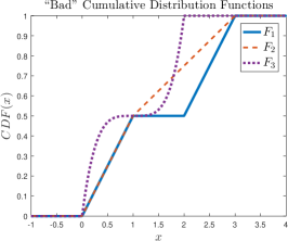
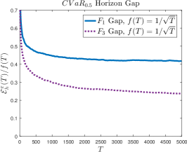
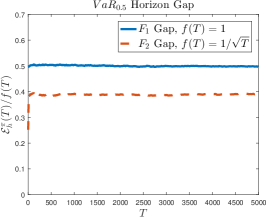
Figure 1: $VaR_{\alpha}$ and $CVaR_{\alpha}$ horizon gap for “bad” distributions. ($F_{1}$) has $\left|L_{0.5}\brk*{F}\right|>1$ and has no density to the right of the percentile; ($F_{2}$) has no density around percentile $\alpha=0.5$; and ($F_{3}$) is not differentiable. The figures essentially show that $\lim_{T\to\infty}J_{1}(T)/f(T)=c>0$ thus claiming that $J_{1}(T)$ behaves as $f(T)$, which is slower than the desired $\mathcal{O}(\frac{\log T}{T})$.

6 Limitations

While our framework encompasses many known performance measures, it has limitations that make it inapplicable to certain potentially interesting examples. The following outlines some of these limitations and indicates how they may be overcome.

No “single optimal arm”.

While all of the examples in Section 5 satisfy this assumption, formally defined in 10, this is not always the case. For example, consider the performance measure

$${U}^{w}\brk 1{F}=\int_{0}^{\infty}w(1-F(x))dx,$$ (22)

which is a type of “distorted risk measure” with distortion function $w:[0,1]\to[0,1]$. If we take $w(p)=p(1-p)$ we get that ${U}^{w}$ is concave and thus typically obtains its maximum in an interior point. More concretely, suppose we have two arms with Bernoulli distributions $F_{1},F_{2}$ with parameters $p_{1}\leq p_{2}$, respectively. Then $\mathcal{D}^{\Delta}$, the set of convex combinations, is exactly the Bernoulli distributions with parameter $p\in[p_{1},p_{2}]$. Next, it is easy to see that for a Bernoulli distribution with parameter $p$, we have that ${U}^{w}\brk 1{F}=p(1-p)$, which is strictly concave and obtains its maximum at $p=1/2$. We conclude that if $1/2\in(p_{1},p_{2})$ then for $\lambda^{*}$ such that $\lambda^{*}p_{1}+(1-\lambda^{*})p_{2}=1/2$

$${U}^{w}\brk 1{\lambda^{*}F_{1}+(1-\lambda^{*})F_{2}}>\max\brk[c]*{{U}^{w}\brk 1{F_{1}},{U}^{w}\brk 1{F_{2}}},$$

which contradicts 10. Overall, the above implies that there is no single-arm infinite horizon oracle policy, i.e., one that always chooses a single arm. An example of an infinite horizon oracle in this setting is one that chooses arm $1$ with probability $\lambda^{*}$ and arm $2$ otherwise.
The above performance measure is admittedly somewhat contrived: it prefers a Bernoulli distribution with $p=1/2$ over one with $p=1$, even though the latter has stochastic dominance over the former. Regardless, it is worth emphasizing here that Proposition 1 holds regardless of 10 and thus it only remains to design a pseudo regret minimization algorithm to obtain $1/\sqrt{T}$ regret. We suspect this could be achieved by a similar UCB-type algorithm that optimizes over all convex combinations of the arms. We note that the resulting optimization problem might be difficult to solve and thus may require additional assumptions to make it computationally tractable.

Unstable performance measures.

As seen in the example of $VaR_{\alpha}$ in Section 5, some performance measures could be unstable without additional assumptions on the arm distributions. The following is another such example. Consider ${U}^{w}$ from 22 with $w(p)=\sqrt{p}$ with $F_{1},F_{2}$ Bernoulli as before. If $p_{1}=0$ then we get that

$${U}^{w}\brk 1{F_{2}}-{U}^{w}\brk 1{F_{1}}=\sqrt{p_{2}}.$$

On the other hand, by the homogeneity of the semi-norm we have that

$$\norm{F_{1}-F_{2}}=\norm{p_{2}\mathds{1}_{[0,1)}}=p_{2}\norm{\mathds{1}_{[0,1)}},$$

and thus for any norm, and $b,q$ there exists $p_{2}$ small enough such that

$${U}^{w}\brk 1{F_{2}}-{U}^{w}\brk 1{F_{1}}=\sqrt{p_{2}}>q\brk*{p_{2}\norm{\mathds{1}_{[0,1)}}+p_{2}^{q}\norm{\mathds{1}_{[0,1)}}^{q}}=q\brk*{\norm{F_{1}-F_{2}}+\norm{F_{1}-F_{2}}^{q}},$$

i.e., ${U}^{w}$ does not satisfy Definition 1. This issue could potentially be overcome by weakening the Lipschitz condition in Definition 1 to a Hölder type condition. This type of change will clearly impact the overall performance result.

Heavy-tailed distributions.

This subject is well understood in the classic bandit setting Bubeck and Cesa-Bianchi (2012), and has also been studied for general learning settings under a $CVaR_{\alpha}$ performance measure Holland and Haress (2020). Our results hold for light-tailed sub-Gaussian arm distributions. We suspect it is possible to extend them to sub-Exponential distributions without significant degradation, but this will not carry over to heavier tails that will likely necessitate a different approach.

7 Open Problems and Future Directions

One main question that we leave open is the dependence of the regret on the number of arms $K$. We conjecture that a finer analysis of the horizon gap may reduce it from our $K^{2}\log K$ to either $K$ or $K\log K$. The subject of lower bounds remains open as well. Future directions may include a more complete taxonomy of performance criteria, or an extension of this framework to different settings (e.g., adversarial or contextual). Additionally, we note that the majority of our proof techniques also apply to non-quasiconvex criteria. If such criteria are found to be of interest then extending the framework to this case may be appealing.

A future direction of great interest is to consider a Markov decision model for the dynamics. The same criteria of interest are still relevant, but now it is unclear whether a simple (Markov) policy could approximate the oracle and if so, at what rate.

sectionappendix

Appendix A EDPMs as Permutation Invariant Performance Measures

The following continues the discussion in Section 2 on the motivation behind EDPMs and their relation to permutation invariant performance measures. Let $\brk[c]1{\tilde{U}_{t}}_{t=1}^{\infty}$, where $\tilde{U}_{t}:\mathbb{R}^{t}\to\mathbb{R}$ is a function that measures the quality of a given reward sequence of length $t$. A decision maker may then wish to maximize the expected performance, i.e., $\mathbf{E}{\tilde{U}_{t}\brk*{X_{{\pi},{1}},\ldots,X_{{\pi},{t}}}}$. It makes sense that the preferences of the decision maker remain fixed over time. This means $\tilde{U}_{t}$ ($t\geq 1$) should, in some sense, be time invariant. However, such an invariance is hard to grasp when the functions $\tilde{U}_{t}$ do not share a domain. One way of addressing this issue is to assume that $\tilde{U}_{t}$ is permutation invariant, i.e., it maps all the permutations of its reward sequence to the same value. We provide a formal definition in the proof of the following (known) result.

Lemma 4 (Permutation invariant function representation).

$\tilde{U}_{t}$ is permutation invariant if and only if, there exists ${U}_{t}:\mathcal{D}\to\mathbb{R}$ such that, $\tilde{U}_{t}\brk*{x_{1},\ldots,x_{t}}={U}_{t}\brk*{\hat{F}_{t}\brk*{x_{1},\ldots,x_{t}}}$, where $\hat{F}_{t}\brk*{\cdot}$ is the empirical distribution mapping defined in 4.

The representation given in Lemma 4 suggests $\mathcal{D}$ as a shared domain thus making it simple to define time invariance. We conclude that EDPMs describe the objectives that are time and permutation invariant.

Proof (of Lemma 4).

We start with a few definitions. Let $\Sigma_{t}$ denote the set of $t\times t$ permutation matrices (binary and doubly stochastic). $\tilde{U}_{t}$ is said to be permutation invariant if $\tilde{U}_{t}\brk*{\sigma x_{1:t}}=\tilde{U}_{t}\brk*{x_{1:t}}$ for all $x_{1:t}\in\mathbb{R}^{t}$ and $\sigma\in\Sigma_{t}$. Let, $\hat{\mathcal{D}}_{t}=\big{\{}\hat{F}_{t}\brk*{x_{1:t}}\;\big{|}\;x_{1:t}\in\mathbb{R}^{t}\big{\}}$, be the set of empirical distributions created from $t$ elements (the image of $\hat{F}_{t}$). Let,

$$\hat{F}_{t}^{-1}\brk*{\hat{F}}=\Big{\{}x_{1:t}\in\mathbb{R}^{t}\;\Big{|}\;\hat{F}_{t}\brk*{x_{1:t}}=\hat{F}\Big{\}},$$

be the inverse image of $\hat{F}_{t}$ at $\hat{F}\in\hat{\mathcal{D}}_{t}$. Let,

$$\Sigma(x_{1:t})=\Big{\{}\sigma x_{1:t}\;\Big{|}\;\sigma\in\Sigma_{t}\Big{\}},$$

be the set of all permutations of $x_{1:t}$. We can now begin the proof.

First direction: Suppose $\tilde{U}_{t}\brk*{x_{1},\ldots,x_{t}}={U}_{t}\brk*{\hat{F}_{t}\brk*{x_{1},\ldots,x_{t}}}$. Notice that $\hat{F}_{t}$ is indeed permutation invariant as permuting its input simply reorders its finite sum thus not changing the value. This clearly implies that $\tilde{U}_{t}$ is permutation invariant.

Second direction: Suppose that $\tilde{U}_{t}$ is permutation invariant. Below, we prove that for any $x_{1:t}\in\mathbb{R}^{t}$

$$\hat{F}_{t}^{-1}\brk*{\hat{F}_{t}\brk*{x_{1:t}})}=\Sigma(x_{1:t}).$$ (23)

Assuming 23 holds true, define $g:\hat{\mathcal{D}}_{t}\to\mathbb{R}^{t}$ in the following way. For any $\hat{F}\in\hat{\mathcal{D}}_{t}$ choose arbitrarily $g\brk*{\hat{F}}\in\hat{F}_{t}^{-1}(\hat{F}))$. Further define ${U}_{t}:\mathcal{D}\to\mathbb{R}$ by,

$${U}_{t}(F)=\begin{cases}\tilde{U}_{t}\brk*{g(F)}&F\in\hat{\mathcal{D}}_{t}\\ 0&\mbox{otherwise.}\end{cases}$$

Then by 23 we have that, $g\brk*{\hat{F}_{t}\brk*{x_{1:t}}}\in\hat{F}_{t}^{-1}\brk*{\hat{F}_{t}\brk*{x_{1:t}}}=\Sigma(x_{1:t})$, and thus there exists $\sigma_{g(x)}\in\Sigma_{t}$, such that $g\brk*{\hat{F}_{t}\brk*{x_{1:t}}}=\sigma_{g(x)}x_{1:t}$. We conclude that,

$${U}_{t}\brk*{\hat{F}_{t}(x_{1:t})}=\tilde{U}_{t}\brk*{g(\hat{F}_{t}(x_{1:t}))}=\tilde{U}_{t}\brk*{\sigma_{g(x)}x_{1:t}}=\tilde{U}_{t}\brk*{x_{1:t}},$$

where the last step uses the permutation invariance of $\tilde{U}_{t}$. We now show that 23 holds, thus concluding the proof.

Proof of 23: Let $y_{1:t}\in\Sigma(x_{1:t})$ then there exists $\sigma\in\Sigma_{t}$ such that $y_{1:t}=\sigma x_{1:t}$. Since $\hat{F}_{t}$ is permutation invariant then,

$$\hat{F}_{t}\brk*{y_{1:t}}=\hat{F}_{t}\brk*{\sigma x_{1:t}}=\hat{F}_{t}\brk*{x_{1:t}}\implies y_{1:t}\in\hat{F}_{t}^{-1}\brk*{\hat{F}_{t}\brk*{x_{1:t}}},$$

and so $\Sigma(x_{1:t})\subseteq\hat{F}_{t}^{-1}\brk*{\hat{F}_{t}\brk*{x_{1:t}}}$. On the other hand, let $y_{1:t}\in\hat{F}_{t}^{-1}\brk*{\hat{F}_{t}\brk*{x_{1:t}}}$, then we have that, $\hat{F}_{t}\brk*{y_{1:t}}=\hat{F}_{t}\brk*{x_{1:t}}$. Take $\sigma_{x}^{*},\sigma_{y}^{*}\in\Sigma_{t}$ such that, $x_{1:t}^{*}=\sigma_{x}^{*}x_{1:t}$, $y_{1:t}^{*}=\sigma_{y}^{*}y_{1:t}$ are sorted in ascending order. Suppose in contradiction that $x_{1:t}^{*}\neq y_{1:t}^{*}$ and let,

$$s_{0}=\min\Big{\{}s\in\brk[c]*{1,\ldots,t}\;\Big{|}\;x_{s_{0}}^{*}\neq y_{s_{0}}^{*}\Big{\}}$$

be the first index where $x_{1:t}^{*}$ and $y_{1:t}^{*}$ differ. Without loss of generality assume that $x_{s_{0}}^{*}<y_{s_{0}}^{*}$, then we have that,

$$\hat{F}_{t}\brk*{y_{1:t}^{*}}(x_{s_{0}}^{*})=\frac{1}{t}\sum_{s=1}^{t}\mathds{I}_{\brk[s]{y_{s}^{*},\infty}}\brk*{x_{s_{0}}^{*}}=\frac{1}{t}\sum_{s=1}^{s_{0}-1}\mathds{I}_{\brk[s]{y_{s}^{*},\infty}}\brk*{x_{s_{0}}^{*}}=\frac{1}{t}\sum_{s=1}^{s_{0}-1}\mathds{I}_{\brk[s]{x_{s}^{*},\infty}}\brk*{x_{s_{0}}^{*}}<\hat{F}_{t}\brk*{x_{1:t}^{*}}\brk*{x_{s_{0}}^{*}},$$

where the strict inequality follows since $\mathds{I}_{\brk[s]{x_{s_{0}}^{*},\infty}}\brk*{x_{s_{0}}^{*}}=1$, and if $s_{0}=1$, then the empty sum is in fact zero. This contradicts $\hat{F}_{t}\brk*{y_{1:t}}=\hat{F}_{t}\brk*{x_{1:t}}$ and so, $x_{1:t}^{*}=y_{1:t}^{*}$. Since, permutation matrices are invertible then, $y_{1:t}={\sigma_{y}^{*}}^{-1}\sigma_{x}^{*}x_{1:t}$. It is well known that ${\sigma_{y}^{*}}^{-1}\sigma_{x}^{*}$ is always a permutation matrix. So, $y_{1:t}\in\Sigma(x_{1:t})$ and we conclude that $\hat{F}_{t}^{-1}\brk*{\hat{F}_{t}\brk*{x_{1:t}}}=\Sigma(x_{1:t})$, as desired.

Appendix B Proofs of Section 4.1

Denote the fraction of time at which arm $i$ was pulled by

$$\hat{p}_{i}\brk*{T}=\frac{\tau_{i}\brk*{T}}{T},$$ (24)

where $\tau_{i}\brk*{T}$ is defined in 2. Recall the definitions of $\hat{F}_{T}^{\pi}$ and $\hat{F}_{T}^{(i)}$ given in 5 and 6. The following Lemma is the main argument of the proof of Theorem 1.

Lemma 5 ($\hat{F}_{T}^{\pi}$ sub-convergence).

Suppose $\lim_{t\to\infty}\norm{\hat{F}_{t}^{(i)}-F^{\brk*{{i}}}}=0$ almost surely $\mbox{for all }i\in\mathds{K}$. Let $p=\brk*{p_{1},\ldots,p_{K}}\in\Delta$ and $\brk[c]*{t_{l}}_{l=1}^{\infty}$ be a random vector and subsequence. If

$$\lim_{l\to\infty}\norm{\hat{p}\brk*{t_{l}}-p}=0\qquad\textit{Almost Surely},$$

Then

$$\lim_{l\to\infty}\norm{\hat{F}_{t_{l}}^{\pi}-F_{p}}=0\qquad\textit{Almost Surely},$$

where $F_{p}$ is defined in 9.

Proof.

We rearrange the expression of $\hat{F}_{T}^{\pi}$ such that the sum is over actions and instead of time:

$$\hat{F}_{T}^{\pi}=\frac{1}{T}\sum_{t=1}^{T}\mathds{I}_{\brk[s]{X_{{\pi},{t}},\infty}}=\sum_{i=1}^{K}\frac{\tau_{i}\brk*{T}}{T}\brk[s]*{\frac{1}{\tau_{i}\brk*{T}}\sum_{t=1}^{\tau_{i}\brk*{T}}\mathds{I}_{\brk[s]{X_{{\pi},{t}},\infty}}}=\sum_{i=1}^{K}\hat{p}_{i}\brk*{T}\hat{F}_{\tau_{i}\brk*{T}}^{(i)}.$$

Then we have that

$$\norm{\hat{F}_{t_{l}}^{\pi}-F_{p}} =\norm{\sum_{i=1}^{K}\hat{p}_{i}\brk*{t_{l}}\hat{F}_{\tau_{i}\brk*{t_{l}}}^{(i)}-p_{i}F^{\brk*{{i}}}}$$

$$=\norm{\brk[s]*{\sum_{i=1}^{K}\hat{p}_{i}\brk*{t_{l}}\hat{F}_{\tau_{i}\brk*{t_{l}}}^{(i)}-\hat{p}_{i}\brk*{t_{l}}F^{\brk*{{i}}}}+\brk[s]*{\sum_{i=1}^{K}\hat{p}_{i}\brk*{t_{l}}F^{\brk*{{i}}}-p_{i}F^{\brk*{{i}}}}}$$

$$\leq\norm{\sum_{i=1}^{K}\hat{p}_{i}\brk*{t_{l}}\brk*{\hat{F}_{\tau_{i}\brk*{t_{l}}}^{(i)}-F^{\brk*{{i}}}}}+\norm{\sum_{i=1}^{K}F^{\brk*{{i}}}\brk*{\hat{p}_{i}\brk*{t_{l}}-p_{i}}}$$

$$\leq\sum_{i=1}^{K}\hat{p}_{i}\brk*{t_{l}}\norm{\hat{F}_{\tau_{i}\brk*{t_{l}}}^{(i)}-F^{\brk*{{i}}}}+\sum_{i=1}^{K}\norm{F^{\brk*{{i}}}}\abs{\hat{p}_{i}\brk*{t_{l}}-p_{i}}$$

$$\leq\sum_{i=1}^{K}\underbrace{\hat{p}_{i}\brk*{t_{l}}\norm{\hat{F}_{\tau_{i}\brk*{t_{l}}}^{(i)}-F^{\brk*{{i}}}}}_{(*)}+\underbrace{K\max_{1\leq i\leq K}{\norm{F^{\brk*{{i}}}}}\norm{\hat{p}\brk*{t_{l}}-p}_{\infty}}_{(**)\to 0}.$$

The first and second inequalities follow by the triangle inequality and homogeneity of norms. The third follows by Hölder’s inequality. By the Lemma’s assumption $(**)\to 0$. We show that the same holds for (*). It is enough to show the convergence of the summands in order to conclude the overall convergence of this finite sum. By the Lemma’s assumption we have that

$$\lim_{l\to\infty}\norm{\hat{F}_{\tau_{i}\brk*{t_{l}}}^{(i)}-F^{\brk*{{i}}}}=\begin{cases}0\quad&,\lim_{l\to\infty}\tau_{i}\brk*{t_{l}}=\infty\\ \norm{\hat{F}_{\tau}^{(i)}-F^{\brk*{{i}}}}\quad&,\lim_{l\to\infty}\tau_{i}\brk*{t_{l}}=\tau<\infty\end{cases}\qquad\textit{Almost Surely},$$

where we used the fact that $\tau_{i}\brk*{t}$ is non-decreasing and thus always converges. Now since both parts of (*) converge then we have that,

$$\lim_{l\to\infty}\hat{p}_{i}\brk*{t_{l}}\norm{\hat{F}_{\tau_{i}\brk*{t_{l}}}^{(i)}-F^{\brk*{{i}}}} =\lim_{l\to\infty}\hat{p}_{i}\brk*{t_{l}}\lim_{l\to\infty}\norm{\hat{F}_{\tau_{i}\brk*{t_{l}}}^{(i)}-F^{\brk*{{i}}}}$$

$$=\begin{cases}0\quad&,\lim_{l\to\infty}\tau_{i}\brk*{t_{l}}=\infty\\ p_{i}\norm{\hat{F}_{\tau}^{(i)}-F^{\brk*{{i}}}}\quad&,\lim_{l\to\infty}\tau_{i}\brk*{t_{l}}=\tau<\infty\end{cases}\qquad\textit{Almost Surely}.$$

Noticing that

$$\lim_{l\to\infty}\tau_{i}\brk*{t_{l}}=\tau<\infty\implies p_{i}=\lim_{l\to\infty}\hat{p}_{i}\brk*{t_{l}}=\lim_{l\to\infty}\frac{\tau_{i}\brk*{t_{l}}}{t_{l}}=0,$$

the proof is concluded.

Proof (of Theorem 1).

The remainder of the proof consists of applying Lemma 5. Let $\pi^{p}$ be a simple randomized policy that at each turn draws an arm $i.i.d$ with distribution $p\in\Delta$, i.e., $\mathbb{P}\brk*{\pi^{p}_{t}=i}=p_{i}$. We begin by proving $\mathbf{E}{{U}_{\pi^{p}}}={U}\brk 1{F_{p}}$. Let $p\in\Delta$ define the simple policy $\pi^{p}$. Using the strong law of large numbers (Simonnet (1996)) on each coordinate of $\hat{p}\brk*{t}$, we conclude that

$$\lim_{t\to\infty}\norm{\hat{p}\brk*{t}-p}_{\infty}=0\qquad\textit{Almost Surely}.$$

Applying Lemma 5 we get that

$$\lim_{t\to\infty}\norm{\hat{F}_{t}^{\pi^{p}}-F_{p}}=0\qquad\textit{Almost Surely}.$$

Since ${U}$ is assumed to be continuous, we have that,

$${U}_{\pi^{p}}=\liminf_{t\to\infty}{U}\brk 1{\hat{F}_{t}^{\pi^{p}}}\overset{a.s}{=}\lim_{l\to\infty}{U}\brk 1{\hat{F}_{t_{l}}^{\pi^{p}}}\overset{a.s}{=}{U}\brk 1{F_{p}},$$

where $\brk[c]*{t_{l}}_{l=1}^{\infty}$ is the (random) subsequence that achieves the limit inferior. Taking expectation, we conclude that $\mathbf{E}{{U}_{\pi^{p}}}={U}\brk 1{F_{p}}$. Now since $\Delta$ is compact and ${U}\brk 1{F_{p}}$ is continuous, then by the Weierstrass theorem we have that there exists $p^{*}\in\Delta$ such that,

$${U}\brk 1{F_{p^{*}}}=\max_{p\in\Delta}{U}\brk 1{F_{p}}.$$ (25)

We now show that $\pi^{p^{*}}$ is optimal thus concluding the first part of the proof. Let $\brk[c]*{t_{m}}_{m=1}^{\infty}$ be a (random) subsequence satisfying the limit inferior. Then we have that

$${U}_{\pi}=\liminf_{t\to\infty}{U}\brk 1{\hat{F}_{t}^{\pi}}\overset{a.s}{=}\lim_{m\to\infty}{U}\brk 1{\hat{F}_{t_{m}}^{\pi}}=(**).$$

Noticing again that $\Delta$ is compact, we have that for any policy $\pi\in\Pi$, there exist $p\in\Delta$ and $\brk[c]*{t_{l}}_{l=1}^{\infty}\subseteq\brk[c]*{t_{m}}_{m=1}^{\infty}$ (both random) satisfying $\lim_{l\to\infty}\norm{\hat{p}\brk*{t_{l}}-p}_{\infty}=0$ almost surely. Using Lemma 5, 25, and the continuity of ${U}$ we get,

$$(**)\overset{a.s}{=}\lim_{l\to\infty}{U}\brk 1{\hat{F}_{t_{l}}^{\pi}}\overset{a.s}{=}{U}\brk 1{F_{p}}\leq{U}\brk 1{F_{p^{*}}}=\mathbf{E}{{U}_{\pi^{p^{*}}}},$$

and taking expectation we have $\mathbf{E}{{U}_{\pi}}\leq\mathbf{E}{{U}_{\pi^{p^{*}}}}$ for all $\pi\in\Pi$, i.e., $\pi^{p^{*}}=\pi^{*}\brk*{\infty}$.

Moving on to the second part of the Theorem, notice that $\Delta$ is convex, compact and its set of extreme points is also compact (discrete). So, returning to 25 and using the quasiconvexity of ${U}$, we notice that a maximizer is attained at an extreme point of $\Delta$. Formally, there exists $i^{*}\in\mathds{K}$ such that

$${U}\brk 1{F_{e_{i^{*}}}}=\max_{p\in\Delta}{U}\brk 1{F_{p}},$$

where $\brk[c]*{e_{i}}_{i=1}^{K}$ are the standard unit vectors in $\mathbb{R}^{K}$. Continuing as before we conclude that $\pi^{e_{i^{*}}}=\pi^{*}\brk*{\infty}$ as desired.

Appendix C Proofs of Section 4.3

Proof (of Lemma 1).

We begin by proving the Lipschitz property. Using the local modulus of continuity assumed by stability we get that for any $F_{1},F_{2}\in\mathcal{D}^{\Delta}$

$$\abs{{U}\brk 1{F_{1}}-{U}\brk 1{F_{2}}} \leq b\brk*{\norm{F_{1}-F_{2}}+\norm{F_{1}-F_{2}}^{q}}$$

$$=b\brk*{1+\norm{F_{1}-F_{2}}^{q-1}}\norm{F_{1}-F_{2}}$$

$$\leq b\brk*{1+D^{q-1}}\norm{F_{1}-F_{2}}$$

$$=L\norm{F_{1}-F_{2}},$$

as desired. Next, we show the pseudo regret decomposition. Using quasiconvexity as in the second part of Theorem 1, there exists $i^{*}\in\mathds{K}$ such that $F_{p^{*}}=F^{(i^{*})}$. Using the Lipschitz constant $L$, and the triangle inequality we thus have that,

$$\bar{R}_{\pi}\brk*{T} =\mathbf{E}\delim{[}{]}*{{U}\brk 1{F^{(i^{*})}}-{U}\brk 1{{F}_{T}^{\pi}}}$$

$$\leq L\mathbf{E}{\norm{F^{(i^{*})}-{F}_{T}^{\pi}}}$$

$$=L\mathbf{E}{\norm{\frac{1}{T}\sum_{i=1}^{K}\tau_{i}\brk*{T}\brk*{F^{(i^{*})}-F^{\brk*{{i}}}}}}$$

$$\leq\frac{L}{T}\mathbf{E}\delim{[}{]}*{\sum_{i=1}^{K}\tau_{i}\brk*{T}\norm{F^{(i^{*})}-F^{\brk*{{i}}}}}$$

$$\leq\frac{L\rho}{T}\sum_{i\neq i^{*}}\Delta_{i}\mathbf{E}{\tau_{i}\brk*{T}}.$$

Proof (of Theorem 2).

The proof uses standard techniques from the UCB literature, and Bubeck and Cesa-Bianchi (2012) in particular. We begin with the following concentration result due to Requirement 2 of stability.

$$\begin{aligned} \mathbb{P}\brk*{\abs{{U}\brk 1{\hat{F}_{t}^{(i)}}-{U}\brk 1{F^{\brk*{{i}}}}}\geq x}&\leq\mathbb{P}\brk*{b\brk*{\norm{\hat{F}_{t}^{(i)}-F^{\brk*{{i}}}}+\norm{\hat{F}_{t}^{(i)}-F^{\brk*{{i}}}}^{q}}\geq x}\\ &\leq\mathbb{P}\brk*{\norm{\hat{F}_{t}^{(i)}-F^{\brk*{{i}}}}\geq\frac{x}{2b}}+\mathbb{P}\brk*{\norm{\hat{F}_{t}^{(i)}-F^{\brk*{{i}}}}\geq\brk*{\frac{x}{2b}}^{1/q}}\\ &\leq 2\exp\brk*{-\upsilon t\brk*{\frac{x}{2b}}^{2}}+2\exp\brk*{-\upsilon t\brk*{\frac{x}{2b}}^{2/q}}\\ &\leq 4\exp\brk*{-t\phi\brk*{x}}.\end{aligned}$$ (26)

Now, for all $i\in\mathds{K}$ and $1\leq t\leq T$ denote the events

$$V_{i}^{t}=\brk[c]*{{U}\brk 1{\hat{F}_{\tau_{i}\brk*{t-1}}^{(i)}}>{U}\brk 1{F^{\brk*{{i}}}}+\phi^{-1}\brk*{\frac{\gamma\log t}{\tau_{i}\brk*{t-1}}}},$$

$$V_{*}^{t}=\brk[c]*{{U}\brk 1{\hat{F}_{\tau_{i^{*}}\brk*{t-1}}^{(i^{*})}}+\phi^{-1}\brk*{\frac{\gamma\log t}{\tau_{i^{*}}\brk*{t-1}}}\leq{U}\brk 1{F^{(i^{*})}}},$$

and their complements by $\overline{V_{i}^{t}}$, $\overline{V_{*}^{t}}$ respectively. Using the union bound and 26 we have that

$$\mathbb{P}\brk*{V_{i}^{t}} =\mathbb{P}\brk*{{U}\brk 1{\hat{F}_{\tau_{i}\brk*{t-1}}^{(i)}}-\phi^{-1}\brk*{\frac{\gamma\log t}{\tau_{i}\brk*{t-1}}}>{U}\brk 1{F^{\brk*{{i}}}}}$$

$$\leq\mathbb{P}\brk*{\max_{1\leq s\leq t}\brk[c]*{{U}\brk 1{\hat{F}_{s}^{(i)}}-\phi^{-1}\brk*{\frac{\gamma\log t}{s}}}>{U}\brk 1{F^{\brk*{{i}}}}}$$

$$\leq\sum_{s=1}^{t}\mathbb{P}\brk*{{U}\brk 1{\hat{F}_{s}^{(i)}}-\phi^{-1}\brk*{\frac{\gamma\log t}{s}}>{U}\brk 1{F^{\brk*{{i}}}}}$$

$$\leq\sum_{s=1}^{t}\mathbb{P}\brk*{\abs{{U}\brk 1{\hat{F}_{s}^{(i)}}-{U}\brk 1{F^{\brk*{{i}}}}}\geq\phi^{-1}\brk*{\frac{\gamma\log t}{s}}}$$

$$\leq\sum_{s=1}^{t}4\exp\brk*{-s\phi\brk*{\phi^{-1}\brk*{\frac{\gamma\log t}{s}}}}$$

$$\leq\sum_{s=1}^{t}\frac{4}{t^{\gamma}}=\frac{4}{t^{\gamma-1}}.$$

The same holds for $\mathbb{P}\brk*{V_{*}^{t}}$, and so we obtain

$$\mathbb{P}\brk*{V_{i}^{t}\cup V_{*}^{t}}\leq\mathbb{P}\brk*{V_{i}^{t}}+\mathbb{P}\brk*{V_{*}^{t}}\leq\frac{8}{t^{\gamma-1}}.$$ (27)

Next, we denote $u={\frac{\gamma\log T}{\phi\brk*{\Delta_{i}/2}}}$, and show that

$$\brk[c]*{\pi^{{U}-UCB}_{t}=i}\cap\brk[c]*{\tau_{i}\brk*{t-1}\geq u}\subseteq V_{i}^{t}\cup V_{*}^{t}.$$ (28)

Indeed, assume in contradiction that $\brk[c]*{\pi^{{U}-UCB}_{t}=i}\cap\brk[c]*{\tau_{i}\brk*{t-1}\geq u}\cap\overline{V_{i}^{t}}\cap\overline{V_{*}^{t}}\neq\emptyset$, then noticing that $\brk[c]*{\tau_{i}\brk*{t-1}\geq u}$ implies $\brk[c]*{\Delta_{i}\geq 2\phi^{-1}\brk*{\frac{\gamma\log t}{\tau_{i}\brk*{t-1}}}}$ we have:

$${U}\brk 1{\hat{F}_{\tau_{i^{*}}\brk*{t-1}}^{(i^{*})}}+\phi^{-1}\brk*{\frac{\gamma\log t}{\tau_{i^{*}}\brk*{t-1}}} >{U}\brk 1{F^{(i^{*})}}$$

$$={U}\brk 1{F^{\brk*{{i}}}}+\Delta_{i}$$

$$\geq{U}\brk 1{F^{\brk*{{i}}}}+2\phi^{-1}\brk*{\frac{\gamma\log t}{\tau_{i}\brk*{t-1}}}$$

$$\geq{U}\brk 1{\hat{F}_{\tau_{i}\brk*{t-1}}^{(i)}}+\phi^{-1}\brk*{\frac{\gamma\log t}{\tau_{i}\brk*{t-1}}},$$

which implies that $\pi^{{U}-UCB}_{T}\neq i$, thus contradicting our assumption. Finally, denoting

$$t_{0}=\max_{1\leq t\leq T}\brk[c]*{t~{}\Big{|}~{}\tau_{i}\brk*{t-1}\leq\max\brk[c]*{u,1}},$$

and using 27 and 28 we have that

$$\mathbf{E}{\tau_{i}\brk*{T}} =\mathbf{E}\delim{[}{]}*{\sum_{t=1}^{T}\mathds{1}{\brk[c]*{\pi^{{U}-UCB}_{t}=i}}}$$

$$=\mathbf{E}\delim{[}{]}*{\sum_{t=1}^{t_{0}}\mathds{1}{\brk[c]*{\pi^{{U}-UCB}_{t}=i}}+\sum_{t=t_{0}+1}^{T}\mathds{1}{\brk[c]*{\pi^{{U}-UCB}_{t}=i}}}$$

$$=\mathbf{E}\delim{[}{]}*{\tau_{i}\brk*{t_{0}}+\sum_{t=t_{0}+1}^{T}\mathds{1}{\brk[c]*{\pi^{{U}-UCB}_{t}=i\bigcap\tau_{i}\brk*{t-1}\geq u}}}$$

$$\leq\mathbf{E}\delim{[}{]}*{u+1+\sum_{t=K+1}^{T}\mathds{1}{\brk[c]*{\pi^{{U}-UCB}_{t}=i\bigcap\tau_{i}\brk*{t-1}\geq u}}}$$

$$=u+1+\sum_{t=K+1}^{T}\mathbb{P}\brk*{\pi^{{U}-UCB}_{t}=i\bigcap\tau_{i}\brk*{t-1}\geq u}$$

$$\leq u+1+\sum_{t=K+1}^{T}\mathbb{P}\brk*{V_{i}^{t}\cup V_{*}^{t}}$$

$$\leq u+1+\sum_{t=K+1}^{T}\frac{8}{t^{\gamma-1}}\leq u+1+\int_{K}^{\infty}\frac{8}{t^{\gamma-1}}dt\leq u+1+\frac{8}{\brk*{\gamma-2}K^{\gamma-2}}\leq u+\frac{\gamma+6}{\gamma-2}.$$

Combining this with the expression for the pseudo regret given in Lemma 1 we obtain the desired.

Appendix D Proofs of Section 4.4

We first need the following technical lemma whose proof may be found in Section D.1.

Lemma 6.

Suppose that Requirement 2 of stability holds. Then for any integer $d\geq 1$, policy $\pi\in\Pi$, and $K,T$ such that $\log KT\geq 3$, we have that:

1. $\mathbf{E}{\norm{\hat{F}_{T}^{\pi}-{F}_{T}^{\pi}}^{d}}\leq\brk[s]{1+dm!}\brk*{\frac{K^{2}\log KT}{\upsilon T}}^{d/2},$ where $m=\delim\lceil\rceil*{\frac{d}{2}-1}$;

2. $\mathbf{E}{\norm{\hat{F}_{T}^{\pi}-{F}_{T}^{\pi}}^{d}}\leq 2\brk*{\frac{K^{2}\log KT}{\upsilon T}}^{1/2}$ for all $T\geq\frac{4dK^{2}\log KT}{\upsilon}$;

3. $\mathbf{E}\delim{[}{]}*{\norm{\hat{F}_{T}^{\pi}-{F}_{T}^{\pi}}^{d}\mathds{1}{\brk[c]1{\norm{\hat{F}_{T}^{\pi}-{F}_{T}^{\pi}}>M}}}\leq\frac{1}{T^{2}}$ for all $T\geq\frac{4dK^{2}\log KT}{\upsilon},M^{2}\geq\frac{4dK^{2}\log KT}{\upsilon T};$

Proof (of Proposition 1).

We use Requirement 1 of stability together with the second part of Lemma 6 to get that

$$\abs 2{\mathbf{E}\delim{[}{]}*{{U}\brk 1{\hat{F}_{T}^{\pi}}-{U}\brk 1{{F}_{T}^{\pi}}}} \leq\mathbf{E}{\abs{{U}\brk 1{\hat{F}_{T}^{\pi}}-{U}\brk 1{{F}_{T}^{\pi}}}}$$

$$\leq b\brk[s]*{\mathbf{E}{\norm{\hat{F}_{T}^{\pi}-{F}_{T}^{\pi}}}+\mathbf{E}{\norm{\hat{F}_{T}^{\pi}-{F}_{T}^{\pi}}^{q}}}$$

$$\leq 4b\brk*{\frac{K^{2}\log KT}{\upsilon T}}^{1/2}.$$

Proof (of Theorem 3).

First, notice that $\mathbf{E}{\hat{F}_{T}^{\pi}}=\mathbf{E}{{F}_{T}^{\pi}}$ for any $\pi\in\Pi$. This is easily seen as,

$$\mathbf{E}{\hat{F}_{T}^{\pi}}=\mathbf{E}\delim{[}{]}*{\frac{1}{T}\sum_{t=1}^{T}\mathds{I}_{\brk[s]{X_{{\pi},{t}},\infty}}}=\mathbf{E}\delim{[}{]}*{\frac{1}{T}\sum_{t=1}^{T}\mathbf{E}\delim{[}{]}*{\mathds{I}_{\brk[s]{X_{{\pi},{t}},\infty}}\big{|}\pi_{t}}}=\mathbf{E}\delim{[}{]}*{\frac{1}{T}\sum_{t=1}^{T}F^{\brk*{{\pi_{t}}}}}=\mathbf{E}{{F}_{T}^{\pi}}.$$

Since $\partial{U}$ is a linear operator, we conclude that

$$\mathbf{E}\delim{[}{]}*{\partial{U}\brk 1{F}\cdot{(\hat{F}_{T}^{\pi}-{F}_{T}^{\pi})}}=0,\qquad\forall F\in\mathcal{D}^{\Delta}.$$

With this in mind, we have the following decomposition

$$\abs*{\mathbf{E}\delim{[}{]}*{{U}\brk 1{\hat{F}_{T}^{\pi}}-{U}\brk 1{{F}_{T}^{\pi}}}} \leq\mathbf{E}{\abs 2{\underbrace{{U}\brk 1{\hat{F}_{T}^{\pi}}-{U}\brk 1{{{F}_{T}^{\pi}}}-\partial{U}\brk 1{{F}_{T}^{\pi}}\cdot{(\hat{F}_{T}^{\pi}-{F}_{T}^{\pi})}}_{\delta_{1}}}}$$

$$+\mathbf{E}{\abs 2{\underbrace{\brk 1{\partial{U}\brk 1{{F}_{T}^{\pi}}-\partial{U}\brk 1{F}}\cdot\brk{\hat{F}_{t}^{\pi}-{F}_{T}^{\pi}}}_{\delta_{2}}}},$$

We bound $\mathbf{E}{\abs{\delta_{1}}},\mathbf{E}{\abs{\delta_{2}}}$ to conclude the proof. For $\mathbf{E}{\abs{\delta_{1}}}$, recalling the parameter $M_{0}$ in Definition 2 (smoothness), we use smoothness together with the first part of Lemma 6 to get that

$$\mathbf{E}\delim{[}{]}*{\abs{\delta_{1}}\mathds{1}{\brk[c]1{\norm{\hat{F}_{T}^{\pi}-{F}_{T}^{\pi}}\leq M_{0}}}}\leq\frac{1}{2}\beta\mathbf{E}\delim{[}{]}*{\norm{\hat{F}_{T}^{\pi}-{F}_{T}^{\pi}}^{2}}\leq\frac{3\beta K^{2}\log KT}{2\upsilon T}.$$

Next, we use stability (modulus of continuity) together with part 3 of Lemma 6, which holds due to our assumption on $M_{0}$, to get that

$$\mathbf{E}\delim{[}{]}*{\abs{\delta_{1}}\mathds{1}{\brk[c]1{\norm{\hat{F}_{T}^{\pi}-{F}_{T}^{\pi}}>M_{0}}}} \leq\mathbf{E}\delim{[}{]}*{\mathds{1}{\brk[c]1{\norm{\hat{F}_{T}^{\pi}-{F}_{T}^{\pi}}>M_{0}}}\brk*{\omega\brk 1{\norm{\hat{F}_{T}^{\pi}-{F}_{T}^{\pi}}}+2b\norm{\hat{F}_{T}^{\pi}-{F}_{T}^{\pi}}}}$$

$$=b\mathbf{E}\delim{[}{]}*{\mathds{1}{\brk[c]1{\norm{\hat{F}_{T}^{\pi}-{F}_{T}^{\pi}}>M_{0}}}\brk*{\norm{\hat{F}_{T}^{\pi}-{F}_{T}^{\pi}}^{q}+3\norm{\hat{F}_{T}^{\pi}-{F}_{T}^{\pi}}}}$$

$$\leq\frac{4b\mathds{1}{\brk[c]*{M_{0}<\infty}}}{T^{2}},$$

where the first step also used the modulus of continuity to bound the Gateaux derivative of ${U}$. Summing the two inequalities bounds $\mathbf{E}{\abs{\delta_{1}}}$.

Finally, to bound $\mathbf{E}{\abs{\delta_{2}}}$ we first use the Cauchy–Schwarz inequality together with smoothness (Definition 2) to get that

$$\mathbf{E}{\abs{\delta_{2}}}\leq\mathbf{E}\delim{[}{]}*{\norm{\partial{U}\brk 1{{F}_{T}^{\pi}}-\partial{U}\brk 1{F}}\norm{\hat{F}_{T}^{\pi}-{F}_{T}^{\pi}}}\leq\beta\mathbf{E}\delim{[}{]}*{\norm{{F}_{T}^{\pi}-F}\norm{\hat{F}_{T}^{\pi}-{F}_{T}^{\pi}}}.$$

Next, let $J_{T}^{2}=\frac{4K^{2}\log KT}{\upsilon T}$ to get that

$$\mathbf{E}\delim{[}{]}*{\abs{\delta_{2}}\mathds{1}{\brk[c]1{\norm{\hat{F}_{T}^{\pi}-{F}_{T}^{\pi}}\leq J_{T}}}}\leq\beta J_{T}\mathbf{E}{\norm{{F}_{T}^{\pi}-F}}.$$

On the other hand, recalling that $D$ is the diameter of $\mathcal{D}^{\Delta}$, we use part 3 of Lemma 6 to get that

$$\mathbf{E}\delim{[}{]}*{\abs{\delta_{2}}\mathds{1}{\brk[c]1{\norm{\hat{F}_{T}^{\pi}-{F}_{T}^{\pi}}>J_{T}}}}\leq\beta D\mathbf{E}\delim{[}{]}*{\norm{\hat{F}_{T}^{\pi}-{F}_{T}^{\pi}}\mathds{1}{\brk[c]1{\norm{\hat{F}_{T}^{\pi}-{F}_{T}^{\pi}}>J_{T}}}}\leq\frac{\beta D}{T^{2}}.$$

Summing the two inequalities bounds $\mathbf{E}{\abs{\delta_{2}}}$, and concludes the proof.

D.1 Technical Side Lemmas

Proof (of Lemma 2).

We start by using the triangle inequality and the union bound to get,

$$\mathbb{P}\brk*{\norm{\hat{F}_{T}^{\pi}-{F}_{T}^{\pi}}>x} =\mathbb{P}\brk*{\norm{\frac{1}{T}\sum_{i=1}^{K}\tau_{i}\brk*{T}\brk*{\hat{F}_{\tau_{i}\brk*{T}}^{(i)}-F^{\brk*{{i}}}}}>x}$$

$$\leq\mathbb{P}\brk*{\frac{1}{T}\sum_{i=1}^{K}\tau_{i}\brk*{T}\norm{\hat{F}_{\tau_{i}\brk*{T}}^{(i)}-F^{\brk*{{i}}}}>x}$$

$$\leq\sum_{i=1}^{K}\mathbb{P}\brk*{\tau_{i}\brk*{T}\norm{\hat{F}_{\tau_{i}\brk*{T}}^{(i)}-F^{\brk*{{i}}}}>\frac{T}{K}x}.$$

Now notice that $0\leq\tau_{i}\brk*{T}\leq T$. So we have that,

$$\tau_{i}\brk*{T}\norm{\hat{F}_{\tau_{i}\brk*{T}}^{(i)}-F^{\brk*{{i}}}}\leq\max_{1\leq s\leq T}s\norm{\hat{F}_{s}^{(i)}-F^{\brk*{{i}}}},$$

where the case of $\tau_{i}\brk*{T}=s=0$ is dropped as it is clearly not the maximizer. Using this expression together with the union bound we get that,

$$\mathbb{P}\brk*{\norm{\hat{F}_{T}^{\pi}-{F}_{T}^{\pi}}>x} \leq\sum_{i=1}^{K}\mathbb{P}\brk*{\max_{1\leq s\leq T}s\norm{\hat{F}_{s}^{(i)}-F^{\brk*{{i}}}}>\frac{T}{K}x}$$

$$\leq\sum_{i=1}^{K}\sum_{s=1}^{T}\mathbb{P}\brk*{\norm{\hat{F}_{s}^{(i)}-F^{\brk*{{i}}}}>\frac{Tx}{sK}}.$$

Applying Requirement 2 of stability (concentration), we have that

$$\begin{aligned} \mathbb{P}\brk*{\norm{\hat{F}_{T}^{\pi}-{F}_{T}^{\pi}}>x}&\leq\sum_{i=1}^{K}\sum_{s=1}^{T}2\exp\brk*{-\upsilon s\brk*{\frac{Tx}{sK}}^{2}}\\ &=2K\sum_{s=1}^{T}\exp\brk*{-\upsilon\frac{T^{2}x^{2}}{sK^{2}}}\\ &\leq 2KT\exp\brk*{-\upsilon\frac{Tx^{2}}{K^{2}}},\end{aligned}$$

where in the last step we use the fact that $s=T$ maximizes the summands.

Proof (of Lemma 6).

For the first claim, recall that $m=\delim\lceil\rceil*{\frac{d}{2}-1},$ and let $x_{0}\geq 0$ be a constant to be determined later. We begin by using the tail sum formula and exchanging variables to get that

$$\mathbf{E}{\norm{\hat{F}_{T}^{\pi}-{F}_{T}^{\pi}}^{d}} =\int_{0}^{\infty}\mathbb{P}\brk*{\norm{\hat{F}_{T}^{\pi}-{F}_{T}^{\pi}}^{d}>x}dx$$

$$\leq x_{0}^{d}+\int_{x_{0}^{d}}^{\infty}\mathbb{P}\brk*{\norm{\hat{F}_{T}^{\pi}-{F}_{T}^{\pi}}^{d}>x}dx$$

$$=x_{0}^{d}+dx_{0}^{d}\int_{1}^{\infty}x^{d-1}\mathbb{P}\brk*{\norm{\hat{F}_{T}^{\pi}-{F}_{T}^{\pi}}>x_{0}x}dx x=(x_{0}x^{\prime})^{d}$$ ()

$$\leq x_{0}^{d}\brk[s]*{1+d\int_{1}^{\infty}x^{2m+1}\mathbb{P}\brk*{\norm{\hat{F}_{T}^{\pi}-{F}_{T}^{\pi}}>x_{0}x}dx},$$

where the last transition used the fact that $2m+1\geq d-1.$ Next, we use the tail bound in Lemma 2 to get that

$$\mathbf{E}{\norm{\hat{F}_{T}^{\pi}-{F}_{T}^{\pi}}^{d}}\leq x_{0}^{d}\brk[s]*{1+2dKT\int_{1}^{\infty}x^{2m+1}\exp\brk*{-\frac{\upsilon Tx_{0}^{2}x^{2}}{K^{2}}}dx.}$$

Now, choose $x_{0}^{2}=\frac{K^{2}\log KT}{\upsilon T},$ and using Lemma 7 with $a=\log KT\geq 3$ to solve this known integral, we get that

$$\mathbf{E}{\norm{\hat{F}_{T}^{\pi}-{F}_{T}^{\pi}}^{d}}\leq\brk[s]*{1+dm!}\brk*{\frac{K^{2}\log KT}{\upsilon T}}^{d/2}.$$

This holds for all $\pi\in\Pi$ thus concluding the proof of the first claim.

Next, we prove the second claim by showing that, under the assumption on $T$, the first claim may be bounded by the desired term. To see this notice that

$$\frac{\brk[s]*{1+dm!}}{2}\brk*{\frac{K^{2}\log KT}{\upsilon T}}^{\frac{d-1}{2}} \leq d^{d/2}\brk*{\frac{K^{2}\log KT}{\upsilon T}}^{\frac{d-1}{2}}$$

$$\leq\frac{d^{1/2}}{4^{(d-1)/2}} T\geq\frac{4dK^{2}\log KT}{\upsilon}$$ ()

$$=\exp{\brk*{\frac{1}{2}\log d-\frac{d-1}{2}\log 4}}$$

$$\leq\exp{\brk*{\frac{d-1}{2}-\frac{d-1}{2}\log 4}}\leq 1. \log x\leq x-1$$ ()

Changing sides gives the desired bound, and concludes the proof of the second claim.

Finally, for the third claim, we begin by repeating the first steps of the first claim to get that

$$\mathbf{E}\delim{[}{]}*{\mathds{1}{\brk[c]1{\norm{\hat{F}_{T}^{\pi}-{F}_{T}^{\pi}}>M}}\norm{\hat{F}_{T}^{\pi}-{F}_{T}^{\pi}}^{d}} \leq\mathbf{E}\delim{[}{]}*{\mathds{1}{\brk[c]1{\norm{\hat{F}_{T}^{\pi}-{F}_{T}^{\pi}}>x_{1}}}\norm{\hat{F}_{T}^{\pi}-{F}_{T}^{\pi}}^{d}}$$

$$\leq 2dx_{1}^{d}KT\int_{1}^{\infty}x^{2m+1}\exp\brk*{-\frac{\upsilon Tx_{1}^{2}x^{2}}{K^{2}}}dx,$$

where we choose $x_{1}^{2}=\frac{4dK^{2}\log KT}{\upsilon T}\leq M.$ Notice that our choice of $T$ ensures that $x_{1}\leq 1$ and thus applying Lemma 7 with $a=4d\log KT\geq 3,$ we get that

$$\mathbf{E}\delim{[}{]}*{\mathds{1}{\brk[c]1{\norm{\hat{F}_{T}^{\pi}-{F}_{T}^{\pi}}>M}}\norm{\hat{F}_{T}^{\pi}-{F}_{T}^{\pi}}^{d}} \leq\frac{dm!}{(KT)^{4d-1}}\leq\frac{1}{T^{2}},$$

where the last step also used the fact that $T\geq d$.

Lemma 7.

For any real $a>0$ and integer $m\geq 0$ we have that

$$\int_{1}^{\infty}x^{2m+1}\exp{(-ax^{2})}dx=\frac{\exp{(-a)}}{2a^{m+1}}\sum_{j=0}^{m}\frac{m!}{j!}a^{j}.$$

If $a\geq 3$ then we also have that

$$\int_{1}^{\infty}x^{2m+1}\exp{(-ax^{2})}dx\leq m!\exp{(-a)}/2.$$

Proof.

Denote $f(m)=\int_{1}^{\infty}x^{2m+1}\exp{(-ax^{2})}dx,$ and use integration by parts to get that

$$f(m)=\frac{m}{a}f(m-1)+\frac{\exp{(-a)}}{2a}.$$

Now, plugging $m=0$ we get that $f(0)=\frac{\exp{(-a)}}{2a}.$ Finally, it is trivial to verify that the suggested solution satisfies the difference equation as well as the initial condition, thus concluding the first part of the proof. For the second part we use the assumption on $a\geq 3$ to upper bound the expression as

$$f(m)\leq\frac{m!\exp{(-a)}}{2a}\sum_{j=0}^{m}\frac{1}{j!}\leq\frac{m!e\exp{(-a)}}{2a}\leq\frac{m!\exp{(-a)}}{2}$$

Appendix E Proofs of Section 4.5

Proof (of Proposition 2).

Recall that for any $F\in\mathcal{D}^{\Delta}$ there exists $p\in\Delta$ such that $F=\sum_{i=1}^{K}p_{i}F^{\brk*{{i}}}$. Now, we use convexity to conclude that

$${U}\brk 1{\sum_{i=1}^{K}p_{i}F^{\brk*{{i}}}}-{U}\brk 1{F^{(i^{*})}} \leq\sum_{i=1}^{K}p_{i}\brk*{{U}\brk 1{F^{\brk*{{i}}}}-{U}\brk 1{F^{(i^{*})}}}$$

$$=-\sum_{i=1}^{K}p_{i}\Delta_{i}\leq-\frac{1}{\rho}\sum_{i=1}^{K}p_{i}\norm{F^{\brk*{{i}}}-F^{(i^{*})}}=-\frac{1}{\rho}\norm{F-F^{(i^{*})}},$$

where $\rho$, which is defined in 14, is finite since $\Delta_{i}>0$ for all $i\neq i^{*}$.

Proof (of Theorem 4).

We begin by stating the explicit condition on the time horizon $T$. Letting $J_{T}^{2}=\frac{4K^{2}\log KT}{\upsilon T},$ we require that $T$ is large enough such that

$$\frac{\rho}{T}\sum_{i\neq i^{*}}\brk*{\frac{\gamma\Delta_{i}\log T}{\phi\brk*{\Delta_{i}/2}}+\frac{\gamma+6}{\gamma-2}\Delta_{i}}\leq J_{T}\leq\min\brk[c]*{\frac{1}{\sqrt{q}},\frac{M_{0}}{\sqrt{q}},\frac{1}{\eta\beta}},$$ (29)

which is indeed polynomial in the problem parameters. The first two terms in the minimum are the basic requirements of Theorem 3, and the third term was chosen such that applying Theorem 3 with $F=F^{(i^{*})}$, we get that

$$J_{1}(T)=\mathbf{E}\delim{[}{]}*{{U}\brk 1{\hat{F}_{T}^{\pi^{*}\brk*{T}}}-{U}\brk 1{{F}_{T}^{\pi^{*}\brk*{T}}}}\leq\frac{2\beta K^{2}\log KT}{\upsilon T}+\frac{1}{\eta}\mathbf{E}{\norm{{F}_{T}^{\pi^{*}\brk*{T}}-F^{(i^{*})}}}+\frac{\beta D+4b\mathds{1}{\brk[c]*{M_{0}<\infty}}}{T^{2}}.$$

Next, notice that the first step in the decomposition of the pseudo regret, which is given in Lemma 1, is $\bar{R}_{\pi}\brk*{T}\leq L\mathbf{E}{\norm{{F}_{T}^{{U}-UCB}-F^{(i^{*})}}},$ and thus the bound in Theorem 2 together with the left hand side of 29 imply that $\mathbf{E}{\norm{{F}_{T}^{{U}-UCB}-F^{(i^{*})}}}\leq J_{T}.$ Applying Theorem 3 with $F=F^{(i^{*})}$ we obtain that

$$J_{3}(T)=\mathbf{E}\delim{[}{]}*{{U}\brk 1{{F}_{T}^{{U}-UCB}}-{U}\brk 1{\hat{F}_{T}^{{U}-UCB}}}\leq\underbrace{\frac{6\beta K^{2}\log KT}{\upsilon T}}_{3\beta J_{T}^{2}/2}+\frac{\beta D+4b\mathds{1}{\brk[c]*{M_{0}<\infty}}}{T^{2}}.$$

Next, using the linear gap assumption we get that

$$J_{2}(T)=\mathbf{E}\delim{[}{]}*{{U}\brk 1{{F}_{T}^{\pi^{*}\brk*{T}}}-{U}\brk 1{F^{(i^{*})}}}\leq-\frac{1}{\eta}\mathbf{E}{\norm{{F}_{T}^{\pi^{*}\brk*{T}}-F^{(i^{*})}}}.$$

Finally, recall that in 13 we decompose the regret as $R_{\pi}\brk*{T}=\bar{R}_{\pi}\brk*{T}+J_{1}(T)+J_{2}(T)+J_{3}(T).$ Combining the above and using Theorem 2 to bound $\bar{R}_{{U}-UCB}\brk*{T}$ concludes the proof.

Appendix F Details of Section 5

In this section we provide the missing details from Section 5. For the most part, our goal is to verify stability and smoothness, which are the conditions for Theorem 4. We note that Theorem 1 will typically hold as long as $\abs{{U}\brk 1{F^{\brk*{{i}}}}}<\infty$. The exception to this rule is $VaR_{\alpha}$, for which we will require an additional assumption for this to hold. However, we also show that a single arm infinite horizon oracle always exists, even without this assumption.

In what follow we continue to operate under Assumption 1, which bounds the rewards. This is mostly to make the exposition more concise, and we state explicitly the places where it is indeed necessary.

F.1 Linear EDPMs

We expand on the application of Hoeffding’s inequality for the stability of linear EDPMs, and note that this could easily be replaced by a sub-Gaussian type assumption. Recall that for a linear EDPM ${U}^{\text{lin}}$, we use the seminorm $\norm{F}=\abs{{U}^{\text{lin}}\brk 1{F}}$. We thus have that

$$\norm{\hat{F}_{t}^{(i)}-F^{\brk*{{i}}}}=\abs{{U}^{\text{lin}}\brk 1{\hat{F}_{t}^{(i)}-F^{\brk*{{i}}}}}=\abs*{\frac{1}{t}\sum_{s=1}^{t}{U}^{\text{lin}}\brk 1{\mathds{I}_{\brk[s]{X_{{i},{s}},\infty}}}-{U}^{\text{lin}}\brk 1{F^{\brk*{{i}}}}},$$

where the last transition used the definition of the empirical distribution in 6, and the linearity of ${U}^{\text{lin}}$. Notice that the linearity of ${U}^{\text{lin}}$ also implies that ${U}^{\text{lin}}\brk 1{F^{\brk*{{i}}}}=\mathbf{E}{{U}^{\text{lin}}\brk 1{\mathds{I}_{\brk[s]{X_{{i},{s}},\infty}}}}.$ We now have a sum of zero mean $i.i.d$ random variables that take values in an interval of squared length

$$\vartheta_{\text{lin}}=\max_{x,y\in\brk[s]{0,1}}\brk[s]*{{U}^{\text{lin}}\brk 1{\mathds{I}_{\brk[s]{x,\infty}}}-{U}^{\text{lin}}\brk 1{\mathds{I}_{\brk[s]{y,\infty}}}}^{2},$$

and thus invoking Hoeffding’s inequality we get that ${U}^{\text{lin}}$ satisfies Requirement 2 of stability with $\upsilon=2/\vartheta_{\text{lin}}$.

F.2 Composite EDPMs

Recall that an EDPM is composite if there exist ${U}^{(1)},\ldots{U}^{(n)}$ and $h:\mathbb{R}^{n}\to\mathbb{R}$ such that

$${U}^{h}\brk 1{F}=h\brk 1{{U}^{(1)}\brk 1{F},\ldots,{U}^{(n)}\brk 1{F}}.$$

For a set $S\subseteq\mathcal{D}$ let

$${U}^{h}\brk 1{S}=\brk[c]*{\brk 1{{U}^{(1)}\brk 1{F},\ldots,{U}^{(n)}\brk 1{F}}\in\mathbb{R}^{n}\Big{|}\;\forall F\in S}.$$

be its image under the linear mappings that compose ${U}^{h}$. Lemma 3 is made formal in the following result.

Lemma 8 (Composite EDPM).

Suppose ${U}^{(1)},\ldots,{U}^{(n)}$ are linear, and stable with parameter $\upsilon_{0}$. Then:

1. If $h$ admits a polynomial local modulus of continuity, i.e., there exist $b>0,q\geq 1$ such that

   $$\abs{h\brk 1{x}-h\brk 1{y}}\leq b\brk*{\norm{x-y}_{2}+\norm{x-y}_{2}^{q}}\qquad,\forall x\in{U}^{h}\brk 1{\mathcal{D}^{\Delta}},y\in{U}^{h}\brk 1{L_{\norm{\cdot}}},$$

   then ${U}^{h}$ is stable with the same $b,q$ and $\upsilon=\frac{\log 2}{n\log 2n}\upsilon_{0}$;

2. If $h$ is locally smooth, i.e., there exist $\beta\geq 0,M_{0}>0$ such that for any $x\in{U}^{h}\brk 1{\mathcal{D}^{\Delta}},y\in{U}^{h}\brk 1{L_{\norm{\cdot}}}$ satisfying $\norm{x-y}_{2}\leq M_{0}$ we have that

   $$\abs{h\brk 1{y}-h\brk 1{x}-\nabla h\brk 1{x}^{T}(y-x)}\leq\frac{\beta}{2}\norm{x-y}_{2}^{2},$$

   then ${U}^{h}$ is smooth with the same parameters;

3. If $h$ is convex then so is ${U}^{h}$.

Proof.

Recall that we consider ${U}^{h}$ under the norm

$$\norm{F}=\norm{{U}^{(1)}\brk 1{F},\ldots,{U}^{(n)}\brk 1{F}}_{2},$$

where $\norm{\cdot}_{2}$ is the $\ell^{2}$ norm on $\mathbb{R}^{n}$. Starting with Requirement 1 of stability, we use the modulus of continuity assumption on $h$ to get that for all $F\in\mathcal{D}^{\Delta}$ and $G\in L_{\norm{\cdot}}$

$$\abs{{U}^{h}\brk 1{F}-{U}^{h}\brk 1{G}} =\abs{h\brk 1{{U}^{(1)}\brk 1{F},\ldots,{U}^{(n)}\brk 1{F}}-h\brk 1{{U}^{(1)}\brk 1{G},\ldots,{U}^{(n)}\brk 1{G}}}$$

$$\leq b\brk{\norm{{U}^{(1)}\brk 1{F-G},\ldots,{U}^{(n)}\brk 1{F-G}}_{2}+\norm{{U}^{(1)}\brk 1{F-G},\ldots,{U}^{(n)}\brk 1{F-G}}_{2}^{q}}$$

$$=b\brk{\norm{F-G}+\norm{F-G}^{q}}.$$

Next, for Requirement 2 we use the stability of the linear EDPMs to get that

$$\mathbb{P}\brk*{\norm{\hat{F}_{t}^{(i)}-F^{\brk*{{i}}}}>x} =\mathbb{P}\brk*{\norm{{U}^{(1)}\brk 1{\hat{F}_{t}^{(i)}-F^{\brk*{{i}}}},\ldots,{U}^{(n)}\brk 1{\hat{F}_{t}^{(i)}-F^{\brk*{{i}}}}}_{2}>x}$$

$$\leq\min\brk[c]*{1,\sum_{j=1}^{n}\mathbb{P}\brk*{\abs{{U}^{(j)}\brk 1{\hat{F}_{t}^{(i)}-F^{\brk*{{i}}}}}>\frac{x}{\sqrt{n}}}}$$ (union bound)

$$\leq\min\brk[c]*{1,2n\exp\brk{-\frac{\upsilon_{0}tx^{2}}{n}}}$$

$$\leq 2\exp\brk{-\frac{\log 2\upsilon_{0}}{n\log 2n}tx^{2}},$$

thus concluding stability of ${U}^{h}$, which is the first claim.

Now, moving on to smoothness, we use to chain rule to get that for any $F\in\mathcal{D}$ and $G\in L_{\norm{\cdot}}$

$$\partial{U}\brk 1{F}\cdot{G}=\partial h\brk 1{{U}^{(1)}\brk 1{F},\ldots,{U}^{(n)}\brk 1{F}}\cdot G=\nabla h\brk 1{{U}^{(1)}\brk 1{F},\ldots,{U}^{(n)}\brk 1{F}}^{T}\brk{{U}^{(1)}\brk 1{G},\ldots,{U}^{(n)}\brk 1{G}},$$

and applying the assumed smoothness of $h$ we get that if $\norm{F-G}\leq M_{0}$ then

$$\abs{{U}^{h}\brk 1{G}-{U}^{h}\brk 1{F}-\partial{U}\brk 1{F}\cdot{(G-F)}}$$

$$\quad=\left|h\brk 1{{U}^{(1)}\brk 1{G},\ldots,{U}^{(n)}\brk 1{G}}-h\brk 1{{U}^{(1)}\brk 1{F},\ldots,{U}^{(n)}\brk 1{F}}\right.$$

$$\qquad\left.-\nabla h\brk 1{{U}^{(1)}\brk 1{F},\ldots,{U}^{(n)}\brk 1{F}}^{T}\brk{{U}^{(1)}\brk 1{G-F},\ldots,{U}^{(n)}\brk 1{G-F}}\right|$$

$$\quad\leq\frac{1}{2}\beta\norm{{U}^{(1)}\brk 1{G-F},\ldots,{U}^{(n)}\brk 1{G-F}}_{2}^{2}$$

$$\quad=\frac{1}{2}\beta\norm{F-G}^{2},$$

thus concluding the smoothness of ${U}^{h}$, which is the second claim.

Finally, if $h$ is convex the ${U}^{h}$ is a linear variable on a convex function and as such convex.

F.2.1 Entropic risk

This is the only example where Assumption 1 is indeed necessary for our framework. We note that this could be removed in the future by expanding our analysis to an exponential family of moduli of continuity. Recall that in terms of Lemma 8, we have that $h(x)=-\frac{1}{\theta}\log x$, which is convex, and $x\in\brk[s]{\exp(-\theta),1}$. Bounding the first derivative, we get that

$$\frac{dh}{dx}(x)=-\frac{1}{\theta x}\implies\abs*{\frac{dh}{dx}(x)}\leq\frac{1}{\theta}\exp(\theta),$$

and thus $h$ is Lipschitz with this constant and has a modulus of continuity with parameters $b=\frac{1}{2\theta}\exp(\theta),q=1.$ Next, recalling the second order charachterization of smoothness, we bound the second derivative, to get that

$$\beta\leq\max_{x\in\brk[s]{\exp(-\theta),1}}\abs*{\frac{d^{2}h}{dx^{2}}(x)}=\max_{x\in\brk[s]{\exp(-\theta),1}}\frac{1}{\theta x^{2}}=\frac{1}{\theta}\exp(2\theta),$$

thus proving the desired properties for Lemma 8.

F.2.2 Variance

Here $h\brk 1{x_{1},x_{2}}=x_{1}^{2}-x_{2}$, which is convex. Next, for the modulus of continuity we have that

$$\abs{h\brk 1{x_{1},x_{2}}-h\brk 1{y_{1},y_{2}}} =\abs{(x_{1}-y_{1})(x_{1}+y_{1})+(y_{2}-x_{2})}$$

$$\leq(x_{1}-y_{1})^{2}+\abs{2x_{1}(x_{1}-y_{1})+(y_{2}-x_{2})}$$

$$\leq\sqrt{1+4x_{1}^{2}}\brk{\norm{x-y}_{2}^{2}+\norm{x-y}_{2}}.$$

Since $(x_{1},x_{2})\in{U}^{h}\brk 1{\mathcal{D}^{\Delta}}$, we can bound $\abs{x_{1}}\leq\max_{i\in\mathds{K}}\abs{{U}^{\text{ave}}\brk 1{F^{\brk*{{i}}}}}.$ Since the reward is also bounded in $\brk[s]{0,1}$ we further have that $\abs{x_{1}}\leq 1$, giving us the constant $b=\sqrt{5}$. Finally, for smoothness we may bound the hessian as,

$$\beta=\max_{x_{1},x_{2}\in\mathbb{R}}\norm{\nabla^{2}h\brk 1{x_{1},x_{2}}}=\norm*{\begin{pmatrix}2&0\\ 0&0\end{pmatrix}}=2.$$

F.2.3 Mean-variance (Markowitz)

Here we have that for $\rho\geq 0$ $h(x,y)=x+\rho(x^{2}-y)$, which is convex. Next, for the modulus of continuity we have that

$$\abs{h\brk 1{x_{1},x_{2}}-h\brk 1{y_{1},y_{2}}} =\abs{\rho(x_{1}-y_{1})(x_{1}+y_{1})+\rho(y_{2}-x_{2})+(x_{1}-y_{1})}$$

$$\leq\rho(x_{1}-y_{1})^{2}+\abs{(2\rho x_{1}+1)(x_{1}-y_{1})+(y_{2}-x_{2})}$$

$$\leq\sqrt{1+(2\rho\abs{x_{1}}+1)^{2}}\brk{\norm{x-y}_{2}^{2}+\norm{x-y}_{2}}.$$

Since $(x_{1},x_{2})\in{U}^{h}\brk 1{\mathcal{D}^{\Delta}}$, we can bound $\abs{x_{1}}\leq\max_{i\in\mathds{K}}\abs{{U}^{\text{ave}}\brk 1{F^{\brk*{{i}}}}}.$ Since the reward is also bounded in $\brk[s]{0,1}$ we further have that $\abs{x_{1}}\leq 1$, giving us the constant $b=2(1+\rho)$. Finally, for smoothness we may bound the hessian as,

$$\beta=\max_{x_{1},x_{2}\in\mathbb{R}}\norm{\nabla^{2}h\brk 1{x_{1},x_{2}}}=\norm*{\begin{pmatrix}2\rho&0\\ 0&0\end{pmatrix}}=2\rho.$$

F.2.4 Sortino ratio

Here we have that for $r\in\mathbb{R}$ and $\varepsilon_{0}>0$

$$h\brk 1{x_{1},x_{2}}=(x_{1}-r)/\sqrt{\varepsilon_{0}-x_{2}}.$$

Linear gap: Let $\lambda\in\Delta$ and $F=\sum_{i=1}^{K}\lambda_{i}F^{\brk*{{i}}}$. We need to show that

$${U}^{\text{So}}\brk 1{F^{(i^{*})}}-{U}^{\text{So}}\brk 1{F}\geq\frac{1}{\eta}\norm{F^{(i^{*})}-F}.$$

Denote $x_{i}={U}^{\text{ave}}\brk 1{F^{\brk*{{i}}}}$, $y_{i}={U}^{\text{TSV}}\brk 1{F^{\brk*{{i}}}}$, and $z_{i}=\sqrt{\varepsilon_{0}-y_{i}}$ . Notice that $z_{i}$ is concave in $x_{i},y_{i}$ and so we have that

$$\sqrt{\varepsilon_{0}-\sum_{i=1}^{K}\lambda_{i}y_{i}}\geq\sum_{i=1}^{K}\lambda_{i}z_{i}.$$

We conclude that

$${U}^{\text{So}}\brk 1{F^{(i^{*})}}-{U}^{\text{So}}\brk 1{F} =h\brk 1{x_{i^{*}},y_{i^{*}}}-h\brk 1{\sum_{i=1}^{K}\lambda_{i}x_{i},\sum_{i=1}^{K}\lambda_{i}y_{i}}$$

$$\geq\frac{x_{i^{*}}-r}{z_{i^{*}}}-\frac{\sum_{i=1}^{K}\lambda_{i}x_{i}-r}{\sum_{i=1}^{K}\lambda_{i}z_{i}}$$

$$=\frac{\sum_{i=1}^{K}\lambda_{i}\brk{z_{i}(x_{i^{*}}-r)-z_{i^{*}}(x_{i}-r)}}{z_{i^{*}}\sum_{j=1}^{K}\lambda_{j}z_{j}}$$

$$=\sum_{i=1}^{K}\lambda_{i}\frac{z_{i}}{\sum_{j=1}^{K}\lambda_{i}z_{i}}\brk{\frac{x_{i^{*}}-r}{z_{i^{*}}}-\frac{x_{i}-r}{z_{i}}}\geq\frac{z_{\text{min}}}{z_{\text{max}}}\sum_{i=1}^{K}\lambda_{i}\Delta_{i},$$

where $z_{\text{min}}=\min_{i\neq i^{*}}z_{i}$ and $z_{\text{max}}=\max_{i\in\mathds{K}}z_{i}.$ Using the gap ratio defined in 14 we get a linear gap with $\eta=\rho z_{\text{max}}/z_{\text{min}}$.

Stability: For $x\in{U}^{\text{So}}\brk 1{\mathcal{D}^{\Delta}}$ and $y\in{U}^{\text{So}}\brk 1{L_{\norm{\cdot}}}$ we have that

$$\abs{h\brk 1{x_{1},x_{2}}-h\brk 1{y_{1},y_{2}}} =\abs*{\frac{x_{1}-r}{\sqrt{\varepsilon_{0}-x_{2}}}-\frac{y_{1}-r}{\sqrt{\varepsilon_{0}-y_{2}}}}$$

$$\leq\abs*{\frac{x_{1}-r}{\sqrt{\varepsilon_{0}-y_{2}}}-\frac{y_{1}-r}{\sqrt{\varepsilon_{0}-y_{2}}}}+\abs*{\frac{x_{1}-r}{\sqrt{\varepsilon_{0}-x_{2}}}-\frac{x_{1}-r}{\sqrt{\varepsilon_{0}-y_{2}}}}$$

$$\leq\frac{\abs{x_{1}-y_{1}}}{\varepsilon_{0}}+\abs{x_{1}-r}\abs*{\frac{\sqrt{\varepsilon_{0}-y_{2}}-\sqrt{\varepsilon_{0}-x_{2}}}{\sqrt{\varepsilon_{0}-x_{2}}\sqrt{\varepsilon_{0}-y_{2}}}}$$

$$\leq\frac{\abs{x_{1}-y_{1}}}{\varepsilon_{0}}+\frac{\abs{x_{1}-r}}{2\varepsilon_{0}^{3/2}}\abs*{y_{2}-x_{2}}$$

$$\leq\sqrt{\frac{1}{\varepsilon_{0}^{2}}+\frac{(x_{1}-r)^{2}}{4\varepsilon_{0}^{3}}}\norm{x-y}_{2}$$

$$\leq\frac{\abs{x_{1}-r}+2}{2\min\brk[c]{\varepsilon_{0},\varepsilon_{0}^{3/2}}}\norm{x-y}_{2}.$$

Since $(x_{1},x_{2})\in{U}^{\text{So}}\brk 1{\mathcal{D}^{\Delta}}$, we can bound $\abs{x_{1}}\leq\max_{i\in\mathds{K}}\abs{{U}^{\text{ave}}\brk 1{F^{\brk*{{i}}}}}.$ Since the reward is also bounded in $\brk[s]{0,1}$ we further have that $\abs{x_{1}}\leq 1$, giving us the constants $b=(\abs{r}+2)/4\min\brk[c]{\varepsilon_{0},\varepsilon_{0}^{3/2}}$ and $q=1$.

Smoothness: First, we calculate the hessian to get that

$$\nabla^{2}h\brk 1{x_{1},x_{2}}=\begin{pmatrix}0&\frac{1}{2\brk*{\varepsilon_{0}-x_{2}}^{3/2}}\\ \frac{1}{2\brk*{\varepsilon_{0}-x_{2}}^{3/2}}&\frac{3\brk*{x_{1}-r}}{4\brk*{\varepsilon_{0}-x_{2}}^{5/2}}\end{pmatrix}.$$

Next, we upper bound its spectral norm to get that. Let $w\in\mathbb{R}^{2}$ be such that $\norm{w}_{2}\leq 1$. Then we have that

$$\abs{w^{T}\nabla h\brk 1{x_{1},x_{2}}w} =\abs*{\frac{w_{1}w_{2}}{(\varepsilon_{0}-x_{2})^{3/2}}+w_{2}^{2}\frac{3(x_{1}-r)}{4(\varepsilon_{0}-x_{2})^{5/2}}}$$

$$\leq\frac{1}{2(\varepsilon_{0}-x_{2})^{3/2}}+\frac{3\abs{x_{1}-r}}{4(\varepsilon_{0}-x_{2})^{5/2}}$$

$$\leq\frac{2\varepsilon_{0}+\abs{x_{1}-r}}{4\varepsilon_{0}^{5/2}}$$

Here we cannot take $M_{0}=\infty$. However, for any $M_{0}<\infty$ we can use the above bound to conclude that the smoothness assumption of Lemma 8 holds with

$$\beta=\frac{2\varepsilon_{0}+D+M_{0}+\abs{r}}{4\varepsilon_{0}^{5/2}},$$

where under the assumption that the reward is in $\brk[s]{0,1}$ we further have that $D=1$.

F.2.5 Sharpe ratio

Here we have that for $r\in\mathbb{R}$ and $\varepsilon_{0}>0$

$$h\brk 1{x_{1},x_{2}}=(x_{1}-r)/\sqrt{\varepsilon_{0}-x_{1}^{2}+x_{2}}.$$

Linear gap: Let $\lambda\in\Delta$ and $F=\sum_{i=1}^{K}\lambda_{i}F^{\brk*{{i}}}$. We need to show that

$${U}^{\text{Sh}}\brk 1{F^{(i^{*})}}-{U}^{\text{Sh}}\brk 1{F}\geq\frac{1}{\eta}\norm{F^{(i^{*})}-F}.$$

Denote $x_{i}={U}^{\text{ave}}\brk 1{F^{\brk*{{i}}}}$, $y_{i}={U}^{\text{sqr}}\brk 1{F^{\brk*{{i}}}}$, and $z_{i}=\sqrt{\varepsilon_{0}-x_{i}^{2}+y_{i}}$ . Notice that $z_{i}$ is concave in $x_{i},y_{i}$ and so we have that

$$\sqrt{\varepsilon_{0}-\brk{\sum_{i=1}^{K}\lambda_{i}x_{i}}^{2}+\sum_{i=1}^{K}\lambda_{i}y_{i}}\geq\sum_{i=1}^{K}\lambda_{i}z_{i}.$$

We conclude that

$${U}^{\text{Sh}}\brk 1{F^{(i^{*})}}-{U}^{\text{Sh}}\brk 1{F} =h\brk 1{x_{i^{*}},y_{i^{*}}}-h\brk 1{\sum_{i=1}^{K}\lambda_{i}x_{i},\sum_{i=1}^{K}\lambda_{i}y_{i}}$$

$$\geq\frac{x_{i^{*}}-r}{z_{i^{*}}}-\frac{\sum_{i=1}^{K}\lambda_{i}x_{i}-r}{\sum_{i=1}^{K}\lambda_{i}z_{i}}$$

$$=\frac{\sum_{i=1}^{K}\lambda_{i}\brk{z_{i}(x_{i^{*}}-r)-z_{i^{*}}(x_{i}-r)}}{z_{i^{*}}\sum_{j=1}^{K}\lambda_{j}z_{j}}$$

$$=\sum_{i=1}^{K}\lambda_{i}\frac{z_{i}}{\sum_{j=1}^{K}\lambda_{i}z_{i}}\brk{\frac{x_{i^{*}}-r}{z_{i^{*}}}-\frac{x_{i}-r}{z_{i}}}\geq\frac{z_{\text{min}}}{z_{\text{max}}}\sum_{i=1}^{K}\lambda_{i}\Delta_{i},$$

where $z_{\text{min}}=\min_{i\neq i^{*}}z_{i}$ and $z_{\text{max}}=\max_{i\in\mathds{K}}z_{i}.$ Using the gap ratio defined in 14 we get a linear gap with $\eta=\rho z_{\text{max}}/z_{\text{min}}$.

Stability: For $x\in{U}^{\text{Sh}}\brk 1{\mathcal{D}^{\Delta}}$ and $y\in{U}^{\text{Sh}}\brk 1{L_{\norm{\cdot}}}$ we have that

$$\abs{h\brk 1{x_{1},x_{2}}-h\brk 1{y_{1},y_{2}}} =\abs*{\frac{x_{1}-r}{\sqrt{\varepsilon_{0}-x_{1}^{2}+x_{2}}}-\frac{y_{1}-r}{\sqrt{\varepsilon_{0}-y_{1}^{2}+y_{2}}}}$$

$$\leq\abs*{\frac{x_{1}-r}{\sqrt{\varepsilon_{0}-y_{1}^{2}+y_{2}}}-\frac{y_{1}-r}{\sqrt{\varepsilon_{0}-y_{1}^{2}+y_{2}}}}+\abs*{\frac{x_{1}-r}{\sqrt{\varepsilon_{0}-x_{1}^{2}+x_{2}}}-\frac{x_{1}-r}{\sqrt{\varepsilon_{0}-y_{1}^{2}+y_{2}}}}$$

$$\leq\frac{\abs{x_{1}-y_{1}}}{\varepsilon_{0}}+\abs{x_{1}-r}\abs*{\frac{\sqrt{\varepsilon_{0}-y_{1}^{2}+y_{2}}-\sqrt{\varepsilon_{0}-x_{1}^{2}+x_{2}}}{\sqrt{\varepsilon_{0}-x_{1}^{2}+x_{2}}\sqrt{\varepsilon_{0}-y_{1}^{2}+y_{2}}}}$$

$$\leq\frac{\abs{x_{1}-y_{1}}}{\varepsilon_{0}}+\frac{\abs{x_{1}-r}}{2\varepsilon_{0}^{3/2}}\abs*{(x_{1}^{2}-y_{1}^{2})+(y_{2}-x_{2})}$$

$$\leq\frac{\abs{x_{1}-y_{1}}}{\varepsilon_{0}}+\abs{x_{1}-r}\abs*{\frac{\sqrt{\varepsilon_{0}-y_{1}^{2}+y_{2}}-\sqrt{\varepsilon_{0}-x_{1}^{2}+x_{2}}}{\sqrt{\varepsilon_{0}-x_{1}^{2}+x_{2}}\sqrt{\varepsilon_{0}-y_{1}^{2}+y_{2}}}}$$

$$\leq\frac{\abs{x_{1}-y_{1}}}{\varepsilon_{0}}+\frac{\abs{x_{1}-r}}{2\varepsilon_{0}^{3/2}}\brk{(x_{1}-y_{1})^{2}+2\abs{x_{1}}\abs{x_{1}-y_{1}}+\abs{y_{2}-x_{2}}}$$

$$\leq\max\brk[c]*{\varepsilon_{0}^{-1},2\varepsilon_{0}^{-3/2}\abs{x_{1}-r}}\brk*{(x_{1}-y_{1})^{2}+(2\abs{x_{1}}+1)\abs{x_{1}-y_{1}}+\abs{y_{2}-x_{2}}}$$

$$\leq 2(1+\abs{x_{1}})\max\brk[c]*{\varepsilon_{0}^{-1},2\varepsilon_{0}^{-3/2}\abs{x_{1}-r}}\brk*{\norm{x-y}_{2}^{2}+\norm{x-y}_{2}}.$$

Since $(x_{1},x_{2})\in{U}^{\text{Sh}}\brk 1{\mathcal{D}^{\Delta}}$, we can bound $\abs{x_{1}}\leq\max_{i\in\mathds{K}}\abs{{U}^{\text{ave}}\brk 1{F^{\brk*{{i}}}}}.$ Since the reward is also bounded in $\brk[s]{0,1}$ we further have that $\abs{x_{1}}\leq 1$, giving us the constants $b=4\max\brk[c]{\varepsilon_{0}^{-1},2\varepsilon_{0}^{-3/2}(\abs{r}+1)}$ and $q=2$.

Smoothness: The idea here is to bound the spectral norm of the hessian. This is very similar to previous examples and in particular to Sortino ratio.

F.3 Non-composite EDPMs.

In this section we show the properties of $VaR_{\alpha}$ and $CVaR_{\alpha}$ required by our framework. Unless stated otherwise, we use the norm defined in 19. We recall the definitions of $CVaR_{\alpha}$ and $VaR_{\alpha}$ from 21 and 18, and specifically that we have that

$${U}^{CVaR_{\alpha}}\brk 1{F}=z^{*}-\frac{1}{\alpha}\int_{-\infty}^{z^{*}}F(x)dx,$$

where $z^{*}={U}^{VaR_{\alpha}}\brk 1{F}$. Before starting, we require the following technical lemma, proved in Section F.3.3.

Lemma 9 ($CVaR_{\alpha}$ and $\mathbf{VaR_{\alpha}}$ bounds).

For any $F,G\in L_{\norm{\cdot}}$ we have that

$$\abs{{U}^{VaR_{\alpha}}\brk 1{F}-{U}^{VaR_{\alpha}}\brk 1{G}}\leq\frac{2\norm{F}+\norm{F-G}}{\min\brk[c]*{\alpha,1-\alpha}},$$

and

$$0\leq{U}^{CVaR_{\alpha}}\brk 1{G}-{U}^{CVaR_{\alpha}}\brk 1{F} +\frac{1}{\alpha}\int_{-\infty}^{{U}^{VaR_{\alpha}}\brk 1{F}}\brk*{G(x)-F(x)}dx$$

$$\leq\frac{1}{\alpha}\norm{F-G}\abs{{U}^{VaR_{\alpha}}\brk 1{F}-{U}^{VaR_{\alpha}}\brk 1{G}}.$$

If additionally 20 holds, $F\in\mathcal{D}^{\Delta}$, and $\norm{F-G}<M_{\alpha}$ then we also have that

$$\abs{{U}^{VaR_{\alpha}}\brk 1{F}-{U}^{VaR_{\alpha}}\brk 1{G}}\leq b_{\alpha}\norm{F-G}_{\infty}.$$

F.3.1 Conditional Value at Risk (CVaR)

The following summarizes the properties of $CVaR_{\alpha}$ required for applying Theorem 4.

Proposition 4 ($\mathbf{CVaR_{\alpha}}$ properties).

We have that:

1. $CVaR_{\alpha}$ is convex;

2. $CVaR_{\alpha}$ is stable with parameters $b={4}/{\alpha\min\brk[c]*{\alpha,1-\alpha}},q=2,\upsilon=2/3;$

3. If 20 holds then $CVaR_{\alpha}$ is smooth with parameters $\beta=2b_{\alpha}/\alpha$ and $M_{0}=M_{\alpha}$.

Proof.

As previously mentioned, convexity follows from 18, which expresses $CVaR_{\alpha}$ as a maximum over linear functions.

Stability. Starting with the easier Requirement 2 of stability, the concentration of $\norm{\hat{F}_{t}^{(i)}-F^{\brk*{{i}}}}_{\infty}$ follows from the Dvoretzky-Kiefer-Wolfowitz inequality (Massart, 1990) with $\upsilon_{0}=2$, and since the other two terms are linear, the same holds for them by Hoeffding’s inequality. As in Lemma 8 (but for max norm), we conclude that Requirement 2 holds with $\upsilon=2\log 2/\log 6\geq 2/3$. Next, for Requirement 1, first notice that

$$\abs*{\frac{1}{\alpha}\int_{-\infty}^{{U}^{VaR_{\alpha}}\brk 1{F}}\brk*{F(x)-G(x)}dx} \leq\abs*{\frac{1}{\alpha}\int_{-\infty}^{0}\brk*{F(x)-G(x)}dx}+\abs*{\frac{1}{\alpha}\int_{0}^{{U}^{VaR_{\alpha}}\brk 1{F}}\brk*{F(x)-G(x)}dx}$$

$$\leq\frac{1}{\alpha}\brk[s]*{\norm{F-G}+\abs{{U}^{VaR_{\alpha}}\brk 1{F}}\norm{F-G}}$$

$$\leq\frac{\norm{F-G}}{\alpha}\brk[s]*{1+\abs{{U}^{VaR_{\alpha}}\brk 1{F}}},$$

and apply this to the second claim of Lemma 9 to get that

$$\abs{{U}^{CVaR_{\alpha}}\brk 1{G}-{U}^{CVaR_{\alpha}}\brk 1{F}}\leq\frac{\norm{F-G}}{\alpha}\brk[s]*{1+\abs{{U}^{VaR_{\alpha}}\brk 1{F}}+\abs{{U}^{VaR_{\alpha}}\brk 1{F}-{U}^{VaR_{\alpha}}\brk 1{G}}}.$$

Finally, using the first part of Lemma 9 we get that

$$\abs{{U}^{CVaR_{\alpha}}\brk 1{G}-{U}^{CVaR_{\alpha}}\brk 1{F}} \leq\frac{\norm{F-G}}{\alpha}\brk[s]*{1+\abs{{U}^{VaR_{\alpha}}\brk 1{F}}+\frac{2\norm{F}+\norm{F-G}}{\min\brk[c]*{\alpha,1-\alpha}}}$$

$$\leq\frac{1}{\alpha}\brk*{1+\abs{{U}^{VaR_{\alpha}}\brk 1{F}}+\frac{\max\brk[c]*{1,2\norm{F}}}{\min\brk[c]*{\alpha,1-\alpha}}}\brk[s]*{\norm{F-G}+\norm{F-G}^{2}},$$

which is Requirement 1 of stability. Further using Assumption 1, we have that $\norm{F},\abs{{U}^{VaR_{\alpha}}\brk 1{F}}\leq 1,$ and plugging this into the above gives the desired value for $b$.

Smoothness. Assume that $\partial{U}^{CVaR_{\alpha}}\brk 1{F}\cdot{G}=-\frac{1}{\alpha}\int_{-\infty}^{{U}^{VaR_{\alpha}}\brk 1{F}}G(x)dx.$ We show that the smoothness condition holds under this assumption, which in turn implies that this assumption must be true (see definition of Frechet derivative). To that end, we use the second and third parts of Lemma 9 to get that for any $F\in\mathcal{D}^{\Delta}$ and $G\in L_{\norm{\cdot}}$ satisfying $\norm{F-G}\leq M_{\alpha}$ we have that

$$\abs*{{U}^{CVaR_{\alpha}}\brk 1{G}-{U}^{CVaR_{\alpha}}\brk 1{F}-\frac{-1}{\alpha}\int_{-\infty}^{{U}^{VaR_{\alpha}}\brk 1{F}}\brk*{G(x)-F(x)}dx}$$

$$\qquad\leq\frac{1}{\alpha}\norm{F-G}\abs{{U}^{VaR_{\alpha}}\brk 1{F}-{U}^{VaR_{\alpha}}\brk 1{G}}$$

$$\qquad\leq\frac{1}{2}\frac{2b_{\alpha}}{\alpha}\norm{F-G}^{2},$$

as desired.

F.3.2 Value at Risk (VaR)

We begin with the following proposition, which proves the needed properties of $VaR_{\alpha}$ to get $\mathcal{O}(1/\sqrt{T})$ regret, as described in Remark 1.

Proposition 5 ($\mathbf{VaR_{\alpha}}$ properties).

We have that:

1. $VaR_{\alpha}$ is quasiconvex;

2. If 20 holds then $VaR_{\alpha}$ is stable with parameters $\upsilon=2/3,q=1,$ and

   $$b=\max\brk[c]*{b_{\alpha},\frac{M_{\alpha}+2}{\min\brk[c]*{\alpha,1-\alpha}M_{\alpha}}}.$$

Proof.

Starting with quasiconvexity, let $F_{1},F_{2}\in\mathcal{D}$ and $\lambda\in\brk[s]*{0,1}$. Denote $F_{\lambda}=\lambda F_{1}+\brk*{1-\lambda}F_{2}$, then by the definition of ${U}^{VaR_{\alpha}}$ we have that

$$F_{\lambda}\brk*{\max\brk[c]*{{U}^{VaR_{\alpha}}\brk 1{F_{1}},{U}^{VaR_{\alpha}}\brk 1{F_{2}}}} =\lambda F_{1}\brk*{\max\brk[c]*{{U}^{VaR_{\alpha}}\brk 1{F_{1}},{U}^{VaR_{\alpha}}\brk 1{F_{2}}}}$$

$$\quad+\brk*{1-\lambda}F_{2}\brk*{\max\brk[c]*{{U}^{VaR_{\alpha}}\brk 1{F_{1}},{U}^{VaR_{\alpha}}\brk 1{F_{2}}}}\geq\alpha.$$

Using the definition of ${U}^{VaR_{\alpha}}$ another time we conclude that

$${U}^{VaR_{\alpha}}\brk 1{F_{\lambda}}\leq\max\brk[c]*{{U}^{VaR_{\alpha}}\brk 1{F_{1}},{U}^{VaR_{\alpha}}\brk 1{F_{2}}},$$

which is one of the characterizations of quasiconvexity.

Stability. Since we use the same norm as $CVaR_{\alpha}$, Requirement 2 is proven by Proposition 4. As for Requirement 1, if $\norm{F-G}<M_{\alpha}$ then using the third part of Lemma 9 we have that

$$\abs{{U}^{VaR_{\alpha}}\brk 1{F}-{U}^{VaR_{\alpha}}\brk 1{G}}\leq b_{\alpha}\norm{F-G}.$$

On the other hand, if $\norm{F-G}\geq M_{\alpha}$ then using the first part of Lemma 9 we have that

$$\abs{{U}^{VaR_{\alpha}}\brk 1{F}-{U}^{VaR_{\alpha}}\brk 1{G}} \leq\frac{2\norm{F}+\norm{F-G}}{\min\brk[c]*{\alpha,1-\alpha}}$$

$$=\frac{\norm{F-G}\brk*{1+\frac{2\norm{F}}{\norm{F-G}}}}{\min\brk[c]*{\alpha,1-\alpha}}$$

$$\leq\frac{1+\frac{2\norm{F}}{M_{\alpha}}}{\min\brk[c]*{\alpha,1-\alpha}}\norm{F-G},$$

and combining both results we obtain get that stability holds with $q=1$ and

$$b=\max\brk[c]*{b_{\alpha},\frac{M_{\alpha}+2\norm{F}}{\min\brk[c]*{\alpha,1-\alpha}M_{\alpha}}}.$$

Further using Assumption 1, we have that $\norm{F}\leq 1$, which gives the desired value of $b$.

The following result shows when $VaR_{\alpha}$ satisfies the conditions of Theorem 1, and thus has a single arm infinite horizon oracle policy. We note that this holds regardless as shown Proposition 3, which uses a different approach that is specific to $VaR_{\alpha}$. Denote the $\alpha$ level set of a function $F\in\mathcal{D}$ by $L_{\alpha}\brk*{F}=\brk[c]{x\in\mathbb{R}\big{|}F(x)=\alpha}.$

Proposition 6 ($\mathbf{VaR_{\alpha}}$ Theorem 1 conditions).

If $\abs{L_{\alpha}\brk*{\alpha}}\leq 1$ for all $F\in\mathcal{D}^{\Delta}$. Then ${U}^{VaR_{\alpha}}$ satisfies then conditions of Theorem 1, and thus has a single arm infinite horizon oracle policy.

Proof.

Unlike the remainder of this section, here we use the norm $\norm{F}=\norm{F}_{\infty}$. By the Glivenko-Cantelli theorem Van der Vaart (2000), the convergence of the empirical distribution required in Theorem 1 is established. It thus remains to show that $VaR_{\alpha}$ is continuous on $\mathcal{D}^{\Delta}$. Our condition on the level set can be interpreted in the following way. For any fixed $F\in\mathcal{D}^{\Delta}$

$$y>{U}^{VaR_{\alpha}}\brk 1{F}\implies\exists c_{y}>0,~{}s.t,~{}F(y)\geq\alpha+c_{y}$$ (30)

$$y<{U}^{VaR_{\alpha}}\brk 1{F}\implies\exists c_{y}>0,~{}s.t,~{}F(y)\leq\alpha-c_{y}.$$ (31)

Let $g:[-\frac{\alpha}{2},\frac{1-\alpha}{2}]\to\mathbb{R}$ be given by, $g(\delta)={U}^{VaR_{\alpha+\delta}}\brk 1{F}.$ We show that $g$ is continuous at $0$. $g$ is monotone non decreasing and so has left and right limits at $0$. Let $\brk[c]*{\delta_{n}}_{n=1}^{\infty}\searrow 0$ and denote,

$$\lim_{n\to\infty}g(\delta_{n})=a^{+}.$$

By the monotonicity of $g$ we have that $a^{+}\geq g(0)$. Using 30 we have that, for any $\varepsilon>0$,

$$F(g(0)+\varepsilon)\geq\alpha+c_{\varepsilon},$$

where $c_{\varepsilon}>0$. So, by the expression of ${U}^{VaR_{\alpha}}$, we have that,

$$g(0)+\varepsilon\geq g(c_{\varepsilon})\geq a^{+},$$

where the second inequality follows by the monotonicity of $g$. So, $g(0)\leq a^{+}\leq g(0)+\varepsilon$ for all $\varepsilon>0$ and so $a^{+}=g(0)$. Now take $\brk[c]*{\bar{\delta}_{n}}_{n=1}^{\infty}\nearrow 0$ and denote,

$$\lim_{n\to\infty}g(\bar{\delta}_{n})=a^{-}.$$

A similar set of arguments shows that $a^{-}=g(0)$, and so $g$ is continuous at $0$.

By the continuity of $g$, for any $\varepsilon>0$, there exists $\delta_{\varepsilon}>0$ such that for all $\abs{\beta}\leq\delta_{\varepsilon}$ we have that,

$$\abs{g(0)-g(\beta)}\leq\varepsilon.$$

For any $G\in L_{\norm{\cdot}}$ satisfying $\norm{F-G}_{\infty}\leq\delta_{\varepsilon}$ we have that,

$${U}^{VaR_{\alpha}}\brk 1{F}-{U}^{VaR_{\alpha}}\brk 1{G} =g(0)-\min\Big{\{}y\;\Big{|}\;G(y)\geq\alpha\Big{\}}$$

$$\leq g(0)-\min\Big{\{}y\;\Big{|}\;F(y)\geq\alpha-\delta_{\varepsilon}\Big{\}}=g(0)-g(-\delta_{\varepsilon})\leq\varepsilon.$$

We also have,

$${U}^{VaR_{\alpha}}\brk 1{G}-{U}^{VaR_{\alpha}}\brk 1{F} =\min\Big{\{}y\;\Big{|}\;G(y)\geq\alpha\Big{\}}-g(0)$$

$$\leq\min\Big{\{}y\;\Big{|}\;F(y)\geq\alpha+\delta_{\varepsilon}\Big{\}}-g(0)=g(\delta_{\varepsilon})-g(0)\leq\varepsilon.$$

We conclude that, $\abs{{U}^{VaR_{\alpha}}\brk 1{F}-{U}^{VaR_{\alpha}}\brk 1{G}}\leq\varepsilon$ thus concluding the continuity of ${U}^{VaR_{\alpha}}$ on $\mathcal{D}^{\Delta}$.

Finally, we prove Proposition 3, showing that $VaR_{\alpha}$ always has a single arm infinite horizon oracle policy.

Proof (of Proposition 3).

We begin calculating the performance of a single arm policy. We then proceed to show that the performance of any policy is upper bounded by that of the best single arm policy.

Performance of simple policies. Let $\pi^{i}$ be the policy that always plays arm $i$. We claim that, $\mathbf{E}{{U}_{\pi^{i}}^{VaR_{\alpha}}}={U}^{VaR_{\alpha}}\brk 1{F^{\brk*{{i}}}}.$ If $F^{\brk*{{i}}}$ represents a degenerate random variable then the expression holds trivially. Otherwise, let $y<{U}^{VaR_{\alpha}}\brk 1{F^{\brk*{{i}}}}=a_{i}$, then there exists $\delta_{y}>0$, such that, $F^{\brk*{{i}}}(y)\leq\alpha-\delta_{y}$. Using the strong law of large numbers Simonnet (1996) we have that

$$\lim_{t\to\infty}\hat{F}_{t}^{\pi^{i}}(y)\overset{a.s}{=}F^{\brk*{{i}}}(y)\leq\alpha-\delta_{y}.$$

Let $E$ be the event on which the convergence occurs. Then $\forall\omega\in E$ there exists $T(\omega)$ such that $\forall t>T(\omega)$, we have that,

$$\hat{F}_{t}^{\pi^{i}}(y,\omega)\leq F^{\brk*{{i}}}(y)+\delta_{y}/2\leq\alpha-\delta_{y}/2<\alpha.$$

This implies that ${U}^{VaR_{\alpha}}\brk 1{\hat{F}_{t}^{\pi^{i}}(\omega)}>y$ for all $t\geq T(\omega)$. We get that ${U}_{\pi^{i}}^{VaR_{\alpha}}\geq y$ almost surely, and taking the expectation we get $\mathbf{E}{{U}_{\pi^{i}}^{VaR_{\alpha}}}\geq y$. Since this holds for all $y<{U}^{VaR_{\alpha}}\brk 1{F^{\brk*{{i}}}}$, then,

$$\mathbf{E}{{U}_{\pi^{i}}^{VaR_{\alpha}}}\geq{U}^{VaR_{\alpha}}\brk 1{F^{\brk*{{i}}}}.$$ (32)

On the other hand, using the Law of the iterated logarithm Klenke (2014) we get that

$$\limsup_{t\to\infty}\frac{t}{\lambda\sqrt{2t\log\log t}}\brk*{\hat{F}_{t}^{\pi^{i}}(a_{i})-F^{\brk*{{i}}}(a_{i})}=1\quad a.s,$$

where, $\lambda=F^{\brk*{{i}}}(a_{i})\brk*{1-F^{\brk*{{i}}}(a_{i})}\neq 0$ since $F^{\brk*{{i}}}$ is non-degenerate. We conclude that

$$\hat{F}_{t}^{\pi^{i}}(a_{i})>F^{\brk*{{i}}}(a_{i})\geq\alpha\quad i.o,$$

and thus

$${U}_{\pi^{i}}^{VaR_{\alpha}}=\liminf_{t\to\infty}{U}^{VaR_{\alpha}}\brk 1{\hat{F}_{t}^{\pi^{i}}}\leq a_{i}\quad a.s.$$ (33)

Taking expectation on both sides, we conclude that

$$\mathbf{E}{{U}_{\pi^{i}}^{VaR_{\alpha}}}\leq{U}^{VaR_{\alpha}}\brk 1{F^{\brk*{{i}}}},$$

which together with 32 proves that $\mathbf{E}{{U}_{\pi^{i}}^{VaR_{\alpha}}}={U}^{VaR_{\alpha}}\brk 1{F^{\brk*{{i}}}}.$ Now, recall that in Proposition 5 we showed that ${U}^{VaR_{\alpha}}$ is quasiconvex. We thus have that there exists $i^{*}\in\mathds{K}$ such that for all $F\in\mathcal{D}^{\Delta}$

$${U}^{VaR_{\alpha}}\brk 1{F}\leq{U}^{VaR_{\alpha}}\brk 1{F^{(i^{*})}}=\mathbf{E}{{U}_{\pi^{i^{*}}}^{VaR_{\alpha}}}=a^{*}.$$ (34)

Global optimizer. Our purpose will be to show that

$$\hat{F}_{t}^{\pi}(a^{*})-\alpha>0\quad i.o.$$ (35)

Similarly to 33, this implies that

$${U}_{\pi}^{VaR_{\alpha}}\leq a^{*}\quad a.s,$$

and taking the expectation we conclude that, $\mathbf{E}{{U}_{\pi}^{VaR_{\alpha}}}\leq\mathbf{E}{{U}_{\pi^{i^{*}}}^{VaR_{\alpha}}},$ thus concluding the proof.

By 34, we have that

$${F}_{t}^{\pi}(a^{*})=\frac{1}{t}\sum_{s=1}^{t}F^{\brk*{{\pi_{s}}}}(a^{*})\geq\alpha.$$

We thus get that,

$$\hat{F}_{t}^{\pi}(a^{*})-\alpha\geq\hat{F}_{t}^{\pi}(a^{*})-{F}_{t}^{\pi}(a^{*})=\frac{1}{t}\sum_{s=1}^{t}\mathds{1}{\brk[c]*{X_{{\pi},{s}}\leq a^{*}}}-F^{\brk*{{\pi_{s}}}}(a^{*})=\frac{1}{t}\sum_{s=1}^{t}Y_{s}=\frac{1}{t}W_{t},$$ (36)

where $Y_{s}=\brk[s]*{\mathds{1}{\brk[c]*{X_{{\pi},{s}}\leq a^{*}}}-F^{\brk*{{\pi_{s}}}}(a^{*})}$ and $W_{t}=\sum_{s=1}^{t}Y_{s}$. We split our remaining analysis into two cases.

The first is when policy $\pi$ chooses some non-degenerate arm infinitely often (i.o). For this case we use the Law of the iterated logarithm for martingales given in Fisher (1992). We use the same notation as in Fisher (1992) aside for denoting the martingale $W_{t}$ instead of $U_{t}$, and its difference sequence by $Y_{t}$ instead of $X_{t}$ (to avoid confusion with existing notation). We start by showing $W_{t}$ is a martingale with respect to its natural filtration

$$\mathbf{E}\delim{[}{]}*{W_{t+1}|W_{1},\ldots,W_{t}}$$

$$\quad=W_{t}+\mathbf{E}\delim{[}{]}*{Y_{t+1}|W_{1},\ldots,W_{t}}$$

$$\quad=W_{t}+\mathbf{E}\delim{[}{]}*{\mathbf{E}\delim{[}{]}*{Y_{t+1}|\pi_{t+1}}|W_{1},\ldots,W_{t}}$$

$$\quad=W_{t}+\mathbf{E}\delim{[}{]}*{0|W_{1},\ldots,W_{t}}=W_{t},$$

where the second equality is the law of total probability in addition to $Y_{t+1}|\pi_{t+1}$ being independent of $W_{1},\ldots,W_{t}$. Furthermore, $\mathbf{E}{\abs{W_{t}}}\leq t<\infty$, so $W_{t}$ is a martingale.

Next, let $s_{t}^{2}=\sum_{s=1}^{t}\mathbf{E}\delim{[}{]}*{Y_{s}^{2}|W_{1},\ldots,W_{s-1}}$. Since $\pi$ chooses a non-degenerate arm infinitely often then, $s_{t}^{2}\to\infty$.

Finally, let $t_{0}$ denote the first time $\pi$ chooses a non-degenerate arm. So, we can choose $K_{t}$ in the following way,

$$K_{t}=\varphi(s_{t_{0}})/s_{t_{0}}.$$

Clearly, there exists $K>0$ such that, $\limsup_{t\to\infty}K_{t}<K$. Furthermore,

$$\abs{Y_{t}}\leq\begin{cases}0,&t<t_{0}\\ 1,&t\geq t_{0}\end{cases}\leq K_{t}s_{t}/\varphi(s_{t}).$$

So the conditions of Theorem 1 in Fisher (1992) are met and we conclude that

$$\limsup_{t\to\infty}W_{t}/s_{t}\varphi(s_{t})>0\quad a.s.$$

This means that, $W_{t}>0$ infinitely often and substituting into 36 we conclude that 35 holds.

In the second case, any non-degenerate arm is chosen a finite number of times. Let $i_{b}$ denote the index of the largest degenerate arm and $a_{b}$ be its value. Clearly,

$$a_{b}=\mathbf{E}{{U}_{\pi^{i_{b}}}^{VaR_{\alpha}}}\leq\mathbf{E}{{U}_{\pi^{e_{i^{*}}}}^{VaR_{\alpha}}}=a^{*}.$$

Denote, $I_{b}=\Big{\{}i\;\Big{|}\;F^{\brk*{{i}}}\text{ is degenerate}\Big{\}}$. Since non-degenerate arms are pulled a finite number of times then,

$$\lim_{t\to\infty}\hat{p}_{i}\brk*{t}=0\quad,\forall i\notin I_{b},$$

where $\hat{p}_{i}\brk*{t}$ is defined in 24. Since there are finitely many arms, this implies that

$$\lim_{t\to\infty}\sum_{i\in I_{b}}\hat{p}_{i}\brk*{t}=1.$$

Now, since $a_{b}$ is such that $F^{\brk*{{i}}}(a_{b})=\hat{F}_{t}^{(i)}(a_{b})=1$ for all $i\in I_{b}$, we conclude that

$$\lim_{t\to\infty}\hat{F}_{t}^{\pi}(a^{*}) \geq\lim_{t\to\infty}\hat{F}_{t}^{\pi}(a_{b})$$

$$=\lim_{t\to\infty}\sum_{i=1}^{K}\hat{p}_{i}\brk*{t}\hat{F}_{t}^{(i)}(a_{b})$$

$$\geq\lim_{t\to\infty}\sum_{i\in I_{b}}\hat{p}_{i}\brk*{t}\hat{F}_{t}^{(i)}(a_{b})$$

$$=\lim_{t\to\infty}\sum_{i\in I_{b}}\hat{p}_{i}\brk*{t}=1.$$

Since $\alpha<1$, we can clearly conclude 35 holds, thus finishing the proof.

F.3.3 Proof of Lemma 9

We prove the individual claims of Lemma 9.

First claim. We start by showing that for all $G\in L_{\norm{\cdot}}$

$$\abs{{U}^{VaR_{\alpha}}\brk 1{G}}\leq\frac{\norm{G}}{\min\brk[c]*{\alpha,1-\alpha}}.$$ (37)

Suppose that ${U}^{VaR_{\alpha}}\brk 1{G}\geq 0$, then we have that

$$\norm{G}\geq\int_{0}^{\infty}\brk*{1-G(y)}dy \geq\int_{0}^{{U}^{VaR_{\alpha}}\brk 1{G}}\brk*{1-G(y)}dy$$

$$\geq\int_{0}^{{U}^{VaR_{\alpha}}\brk 1{G}}\brk*{1-\alpha}dy=\brk*{1-\alpha}{U}^{VaR_{\alpha}}\brk 1{G}\geq 0.$$

On the other hand, suppose that ${U}^{VaR_{\alpha}}\brk 1{G}\leq 0$, then we have that

$$\norm{G}\geq\int_{-\infty}^{0}G(y)dy \geq\int_{{U}^{VaR_{\alpha}}\brk 1{G}}^{0}G(y)dy$$

$$\geq\int_{{U}^{VaR_{\alpha}}\brk 1{G}}^{0}\alpha dy=-\alpha{U}^{VaR_{\alpha}}\brk 1{G}\geq 0,$$

thus concluding 37. Using this result, we have that for all $F,G\in L_{\norm{\cdot}}$

$$\abs{{U}^{VaR_{\alpha}}\brk 1{F}-{U}^{VaR_{\alpha}}\brk 1{G}} \leq\abs{{U}^{VaR_{\alpha}}\brk 1{F}}+\abs{{U}^{VaR_{\alpha}}\brk 1{G}}$$

$$\leq\frac{\norm{F}+\norm{G}}{\min\brk[c]*{\alpha,1-\alpha}}$$

$$\leq\frac{2\norm{F}+\norm{F-G}}{\min\brk[c]*{\alpha,1-\alpha}},$$

as desired.

Second claim. We have that

$${U}^{CVaR_{\alpha}}\brk 1{G}-{U}^{CVaR_{\alpha}}\brk 1{F}$$

$$={U}^{VaR_{\alpha}}\brk 1{G}-\frac{1}{\alpha}\int_{-\infty}^{{U}^{VaR_{\alpha}}\brk 1{G}}G(y)dy-{U}^{VaR_{\alpha}}\brk 1{F}+\frac{1}{\alpha}\int_{-\infty}^{{U}^{VaR_{\alpha}}\brk 1{F}}F(y)dy$$

$$={U}^{VaR_{\alpha}}\brk 1{G}-{U}^{VaR_{\alpha}}\brk 1{F}+\frac{1}{\alpha}\int_{{U}^{VaR_{\alpha}}\brk 1{G}}^{{U}^{VaR_{\alpha}}\brk 1{F}}G(y)dy-\frac{1}{\alpha}\int_{-\infty}^{{U}^{VaR_{\alpha}}\brk 1{F}}\brk*{G(y)-F(y)}dy$$

$$=\frac{1}{\alpha}\int_{{U}^{VaR_{\alpha}}\brk 1{G}}^{{U}^{VaR_{\alpha}}\brk 1{F}}\brk*{G(y)-\alpha}dy-\frac{1}{\alpha}\int_{-\infty}^{{U}^{VaR_{\alpha}}\brk 1{F}}\brk*{G(y)-F(y)}dy,$$

and changing sides we get

$${U}^{CVaR_{\alpha}}\brk 1{G}-{U}^{CVaR_{\alpha}}\brk 1{F}+\frac{1}{\alpha}\int_{-\infty}^{{U}^{VaR_{\alpha}}\brk 1{F}}\brk*{G(y)-F(y)}dy=\frac{1}{\alpha}\int_{{U}^{VaR_{\alpha}}\brk 1{G}}^{{U}^{VaR_{\alpha}}\brk 1{F}}\brk*{G(y)-\alpha}dy.$$

It therefore suffices to show that

$$0\leq\frac{1}{\alpha}\int_{{U}^{VaR_{\alpha}}\brk 1{G}}^{{U}^{VaR_{\alpha}}\brk 1{F}}\brk*{G(y)-\alpha}dy\leq\frac{1}{\alpha}\norm{F-G}\abs{{U}^{VaR_{\alpha}}\brk 1{F}-{U}^{VaR_{\alpha}}\brk 1{G}}.$$

Beginning with the left inequality, we have that

$$\begin{aligned} &\frac{1}{\alpha}\int_{{U}^{VaR_{\alpha}}\brk 1{G}}^{{U}^{VaR_{\alpha}}\brk 1{F}}\brk*{G(y)-\alpha}dy\\ &\geq\frac{1}{\alpha}\brk*{{U}^{VaR_{\alpha}}\brk 1{F}-{U}^{VaR_{\alpha}}\brk 1{G}}\brk*{G\brk*{\min\brk[c]*{{U}^{VaR_{\alpha}}\brk 1{G},{U}^{VaR_{\alpha}}\brk 1{F}}}-\alpha}\\ &=\begin{cases}\frac{1}{\alpha}\underbrace{\brk*{{U}^{VaR_{\alpha}}\brk 1{F}-{U}^{VaR_{\alpha}}\brk 1{G}}}_{\leq 0}\underbrace{\brk*{G\brk*{{U}^{VaR_{\alpha}}\brk 1{F}}-\alpha}}_{\leq 0},{U}^{VaR_{\alpha}}\brk 1{G}\geq{U}^{VaR_{\alpha}}\brk 1{F}\\ \frac{1}{\alpha}\underbrace{\brk*{{U}^{VaR_{\alpha}}\brk 1{F}-{U}^{VaR_{\alpha}}\brk 1{G}}}_{\geq 0}\underbrace{\brk*{G\brk*{{U}^{VaR_{\alpha}}\brk 1{G}}-\alpha}}_{\geq 0},{U}^{VaR_{\alpha}}\brk 1{G}<{U}^{VaR_{\alpha}}\brk 1{F}\end{cases}\\ &\geq 0,\end{aligned}$$ (38)

where the final inequality holds since $G(y)\gtreqless\alpha$ for $y\gtreqless{U}^{VaR_{\alpha}}\brk 1{G}$. Next, for the right hand side inequality we have that

$$\frac{1}{\alpha}\int_{{U}^{VaR_{\alpha}}\brk 1{G}}^{{U}^{VaR_{\alpha}}\brk 1{F}}\brk*{G(y)-\alpha}dy$$

$$=\frac{1}{\alpha}\int_{{U}^{VaR_{\alpha}}\brk 1{G}}^{{U}^{VaR_{\alpha}}\brk 1{F}}\brk*{F(y)-\alpha}dy+\frac{1}{\alpha}\int_{{U}^{VaR_{\alpha}}\brk 1{G}}^{{U}^{VaR_{\alpha}}\brk 1{F}}\brk*{G(y)-F(y)}dy$$

$$\leq\underbrace{\frac{1}{\alpha}\int_{{U}^{VaR_{\alpha}}\brk 1{G}}^{{U}^{VaR_{\alpha}}\brk 1{F}}\brk*{F(y)-\alpha}}_{(*)}+\frac{1}{\alpha}\norm{F-G}_{\infty}\abs{{U}^{VaR_{\alpha}}\brk 1{F}-{U}^{VaR_{\alpha}}\brk 1{G}}$$

$$\leq\frac{1}{\alpha}\norm{F-G}\abs{{U}^{VaR_{\alpha}}\brk 1{F}-{U}^{VaR_{\alpha}}\brk 1{G}},$$

where $(*)\leq 0$ is obtained by exchanging the roles of $F$ and $G$ in 38.

Third claim. Consider 20 with $y=\norm{F-G}_{\infty}\leq M_{\alpha}$, and notice that $F\brk*{{U}^{VaR_{\alpha}}\brk 1{F}+y}\geq\alpha$ for any $y\geq 0$. Then we have that

$$F\brk*{{U}^{VaR_{\alpha}}\brk 1{F}+b_{\alpha}\norm{F-G}_{\infty}}-\alpha\geq\norm{F-G}_{\infty}.$$

Using this we get

$$G\brk*{{U}^{VaR_{\alpha}}\brk 1{F}+b_{\alpha}\norm{F-G}_{\infty}}\geq F\brk*{{U}^{VaR_{\alpha}}\brk 1{F}+b_{\alpha}\norm{F-G}_{\infty}}-\norm{F-G}_{\infty}\geq\alpha,$$

which by the definition of ${U}^{VaR_{\alpha}}$ in 21 implies that

$${U}^{VaR_{\alpha}}\brk 1{G}\leq{U}^{VaR_{\alpha}}\brk 1{F}+b_{\alpha}\norm{F-G}_{\infty},$$

and changing sides we get

$${U}^{VaR_{\alpha}}\brk 1{G}-{U}^{VaR_{\alpha}}\brk 1{F}\leq b_{\alpha}\norm{F-G}_{\infty}.$$ (39)

On the other hand, consider 20 with $y=-c\norm{F-G}_{\infty}\geq-M_{\alpha}$, where $1<c\leq\frac{M_{\alpha}}{\norm{F-G}_{\infty}}$. Noticing that $F\brk*{{U}^{VaR_{\alpha}}\brk 1{F}-y}\leq\alpha$ for any $y\geq 0$, we have that

$$-\brk*{F\brk*{{U}^{VaR_{\alpha}}\brk 1{F}-cb_{\alpha}\norm{F-G}_{\infty}}-\alpha}\geq c\norm{F-G}_{\infty},$$

and changing sides we get

$$F\brk*{{U}^{VaR_{\alpha}}\brk 1{F}-cb_{\alpha}\norm{F-G}_{\infty}}\leq\alpha-c\norm{F-G}_{\infty}.$$

Using this we get

$$G\brk*{{U}^{VaR_{\alpha}}\brk 1{F}-cb_{\alpha}\norm{F-G}_{\infty}} \leq F\brk*{{U}^{VaR_{\alpha}}\brk 1{F}-cb_{\alpha}\norm{F-G}_{\infty}}+\norm{F-G}_{\infty}$$

$$\leq\alpha+(1-c)\norm{F-G}_{\infty}$$

$$<\alpha,$$

and using the definition of ${U}^{VaR_{\alpha}}$ in 21 and changing sides we get

$${U}^{VaR_{\alpha}}\brk 1{G}-{U}^{VaR_{\alpha}}\brk 1{F}\geq-cb_{\alpha}\norm{F-G}_{\infty}.$$

Notice that the constant $c$ may be arbitrarily close to $1$. We thus conclude that

$${U}^{VaR_{\alpha}}\brk 1{G}-{U}^{VaR_{\alpha}}\brk 1{F}\geq-b_{\alpha}\norm{F-G}_{\infty},$$

which combined with 39 implies the desired.

F.4 Utility-Based Shortfall Risk (UBSR)

This is a generalization of $VaR_{\alpha}$ that is defined as

$${U}^{UBSR_{\alpha}}\brk 1{F}=\inf_{\xi\in\mathbb{R}}\brk[c]*{\xi~{}\bigg{|}~{}\int_{\mathbb{R}}l(x-\xi)dF(x)\leq\alpha},$$ (40)

where $l:\mathbb{R}\to\mathbb{R}$ is an increasing and $G$ Lipschitz utility function. Under these assumptions, Bhat and Prashanth (2019) show in their Lemma 4 that ${U}^{UBSR_{\alpha}}$ is $G$ Lipschitz with respect to the 1-Wasserstein metric, i.e.,

$$\abs{{U}^{UBSR_{\alpha}}\brk 1{F_{1}}-{U}^{UBSR_{\alpha}}\brk 1{F_{2}}}\leq G\norm{F_{1}-F_{2}}_{1}=G\int_{R}\abs{F_{1}(x)-F_{2}(x)}dx.$$

Moreover, for sub-Gaussian arm distributions, their Lemma 7, which is extracted from Fournier and Guillin (2015), gives the appropriate concentration of the empirical distribution in Wasserstein distance and thus we conclude that it ${U}^{UBSR_{\alpha}}$ is stable. We show that ${U}^{UBSR_{\alpha}}$ is quasi-convex and thus we can apply Propositions 1 and 2 to get that ${U}-UCB$ incurs $\tilde{O}(1/\sqrt{T})$ regret. We suspect that for $l$ that is also smooth and convex it is possible to verify the smoothness and linear gap assumptions and thus invoke Theorem 4 to get $\tilde{O}(\log T/T)$ regret. Unfortunately we did not manage to verify these details formally and thus leave them as a conjecture.
Finally, we verify the quasi-convexity. Let $F_{1},F_{2}$ be two distributions and $\xi_{1},\xi_{2}$ their respective minimizers in ${U}^{UBSR_{\alpha}}$. Assume without loss of generality that $\xi_{1}\leq\xi_{2}$. Since $l$ is increasing we have that for any $\epsilon>0$ and $\lambda\in[0,1]$

$$\int_{\mathbb{R}}l(x-(\xi_{2}+\epsilon)d(\lambda F_{1}+(1-\lambda)F_{2})(x) =\lambda\int_{\mathbb{R}}l(x-(\xi_{2}+\epsilon)dF_{1}(x)+(1-\lambda)\int_{\mathbb{R}}l(x-(\xi_{2}+\epsilon)dF_{2}(x)$$

$$\leq\lambda\int_{\mathbb{R}}l(x-(\xi_{1}+\epsilon)dF_{1}(x)+(1-\lambda)\int_{\mathbb{R}}l(x-(\xi_{2}+\epsilon)dF_{2}(x)$$

$$\leq\lambda\alpha+(1-\lambda)\alpha=\alpha.$$

This implies that $\xi_{2}+\epsilon$ is inside the feasible set of ${U}^{UBSR_{\alpha}}\brk 1{\lambda F_{1}+(1-\lambda)F_{2}}$ for all $\epsilon>0$. We conclude that

$${U}^{UBSR_{\alpha}}\brk 1{\lambda F_{1}+(1-\lambda)F_{2}}\leq\xi_{2}={U}^{UBSR_{\alpha}}\brk 1{F_{2}}=\max\brk[c]*{{U}^{UBSR_{\alpha}}\brk 1{F_{1}},{U}^{UBSR_{\alpha}}\brk 1{F_{2}}},$$

as desired.

F.5 Counter examples

In this section we discuss performance measures for which 10 does not hold. It will thus be necessary to compare performance not to the best single arm policy, but the policy with the best arm mixture. To that end, let $\pi^{p}$ be a simple randomized policy that at each turn draws an arm $i.i.d$ with distribution $p\in\Delta$, i.e., $\mathbb{P}\brk*{\pi^{p}_{t}=i}=p_{i}$.

$\mathbf{{U}^{bad1}}$ details.

Examples such as $VaR_{\alpha}$ are rather uncommon, but, when encountered, their analysis proves challenging. This fact might motivate a more general framework for EDPMs, ideas for which, can be drawn from the proof of Proposition 3. The following examples show the types of problems such frameworks could have or would need to address. Define an EDPM  by,

$${U}^{bad1}\brk 1{F}={U}^{VaR_{0.1}}\brk 1{F}+{U}^{VaR_{0.9}}\brk 1{F},$$

where the values $0.1,~{}0.9$ were chosen arbitrarily. When the two components of ${U}^{bad1}$ are stable then it is clear that so is ${U}^{bad1}$. We show that when this is not the case, then it is possible that no simple policy is optimal. Consider a problem with two arms having the following distributions,

$$F^{\brk*{{1}}}(y)=\begin{cases}0&y<0\\ y/10&0\leq y<1\\ 0.1&1\leq y<5\\ y/50&5\leq y<50\\ 1&y\geq 50\end{cases}\qquad F^{\brk*{{2}}}(y)=\begin{cases}0&y<5\\ 1&y\geq 5.\end{cases}$$

Notice that $F^{(1)}$, $F^{(2)}$ satisfy the conditions of Theorem 1. So, using an intermediate result of Theorem 1 we have that $\lim_{t\to\infty}{U}^{VaR_{0.9}}\brk 1{\hat{F}_{t}^{\pi^{p}}}={U}^{VaR_{0.9}}\brk 1{F_{p}}$ almost surely. Using this convergence we get that

$$\liminf_{t\to\infty}{U}^{bad1}\brk 1{\hat{F}_{t}^{\pi^{p}}} \overset{a.s}{=}\liminf_{t\to\infty}{U}^{VaR_{0.1}}\brk 1{\hat{F}_{t}^{\pi^{p}}}+\lim_{t\to\infty}{U}^{VaR_{0.9}}\brk 1{\hat{F}_{t}^{\pi^{p}}}$$

$$\overset{a.s}{=}{U}^{VaR_{0.1}}\brk 1{F_{p}}+{U}^{VaR_{0.9}}\brk 1{F_{p}}.$$

where the convergence of ${U}^{VaR_{0.1}}\brk 1{\hat{F}_{t}^{\pi^{p}}}$ is an intermediate result in Proposition 3. Evaluating these last terms we conclude the expression for the performance of a simple policy $\pi^{p}$ $(p=(p_{1},p_{2}),~{}p_{1}=1-p_{2})$,

$$\mathbf{E}{{U}_{\pi^{p}}^{bad1}}=\begin{cases}46&p_{2}=0\\ 5+(45-50p_{2})/(1-p_{2})&0<p_{2}<8/9\\ 10&8/9<p_{2}\leq 1\end{cases}$$

It does not attain a maximum over the simplex and thus there is no optimizer inside the set of simple policies. However, the following non-simple policy is optimal,

$$\pi^{*bad1}_{t}=\begin{cases}2&t=1\quad or\quad\frac{\brk*{t-1}\hat{F}_{t-1}^{\pi}(1)+1}{t}\geq 0.1\\ 1&\mbox{otherwise.}\end{cases}$$

We explain why $\pi^{*}_{bad1}$ is an oracle policy. Each of the summands in ${U}^{bad1}$ has a simple oracle policy with appropriate optimal performance. Summing these performances provides an upper bound on the performance of ${U}^{bad1}$. More specifically, ${U}^{bad1}$ is bounded by $50$. We show that, $\pi^{*}_{bad1}$ achieves this value and is thus an oracle policy. It is easy to show by induction that for $(t\geq 1)$, $\hat{F}_{t}^{\pi^{*bad1}}(1)<0.1$. This implies that ${U}^{VaR_{0.1}}\brk 1{\hat{F}_{t}^{\pi^{*bad1}}}\geq 5$, but $5$ is also an upper bound an so, $\liminf_{t\to\infty}{U}^{VaR_{0.1}}\brk 1{\hat{F}_{t}^{\pi^{*bad1}}}=5$. Finally, it is a technical result to show that $\lim_{t\to\infty}\hat{F}_{t}^{\pi^{*bad1}}(5)=0.1$ almost surely, which implies $\lim_{t\to\infty}\hat{p}\brk*{t}\overset{a.s}{=}e_{1}=(1,0)$. Since ${U}^{VaR_{0.9}}$ is stable then this implies that

$$\lim_{t\to\infty}{U}^{VaR_{0.9}}\brk 1{\hat{F}_{t}^{\pi^{*bad1}}}\overset{a.s}{=}{U}^{VaR_{0.9}}\brk 1{F^{\brk*{{1}}}}=45,$$

and taking expectation the result is concluded.

The problem exhibited here is the lack of an optimizer within the set of simple policies. A way of ensuring that this does not occur is to require that the performance of simple policies be upper semi-continuous (with respect to $p$).

$\mathbf{{U}^{bad2}}$ details.

The following example shows that when the performance of simple policies is not lower semi continuous, then while an optimizer exists within the set of simple policies, it might not be a global optimizer. Define an EDPM by,

$${U}^{bad2}\brk 1{F}={U}^{VaR_{0.1}^{++}}\brk 1{F}+5\mathds{1}{\brk[c]*{F({10}^{-})-F({1}^{+})>0~{}or~{}F({1}^{-})>0}},$$

where,

$${U}^{+}\brk 1{F;x}=\max_{y\in\mathbb{R}}\brk[c]*{y\geq x~{}\Big{|}~{}F(y)=F(x)}$$

$${U}^{VaR_{0.1}^{+}}\brk 1{F}=\begin{cases}{U}^{VaR_{0.1}}\brk 1{F}&if~{}F({U}^{VaR_{0.1}}\brk 1{F})=1\\ {U}^{+}\brk 1{F;{U}^{VaR_{0.1}}\brk 1{F}}&otherwise.\end{cases}$$

$${U}^{VaR_{0.1}^{++}}\brk 1{F}=\begin{cases}{U}^{VaR_{0.1}^{+}}\brk 1{F}&if~{}F({U}^{VaR_{0.1}^{+}}\brk 1{F})=1\\ {U}^{+}\brk 1{F;{U}^{VaR_{0.1}^{+}}\brk 1{F}}&otherwise.\end{cases}$$

Consider a problem with two arms having the following distributions,

$$F^{\brk*{{1}}}(y)=\begin{cases}0&y<0\\ 0.9+y/100&0\leq y<10\\ 1&y\geq 10\end{cases}\qquad,F^{\brk*{{2}}}(y)=\begin{cases}0&y<1\\ 0.1&1\leq y<10\\ 1&y\geq 10.\end{cases}$$

The performance of a simple policy $\pi^{p}$ $(p=(p_{1},p_{2}),~{}p_{1}=1-p_{2})$ is given by,

$$\mathbf{E}{{U}_{\pi^{p}}^{bad2}}=\begin{cases}5&p_{2}<8/9\\ -85+10/(1-p_{2})&8/9\leq p_{2}<81/91\\ 6&81/91\leq p_{2}<1\\ 10&p_{2}=1,\end{cases}$$

which attains a maximum for $p_{2}=1$. However, the resulting policy is not an oracle policy. The following non-simple policy is an oracle policy,

$$\pi^{*bad2}_{t}=\begin{cases}1&t=1\\ 2&otherwise.\end{cases}$$

To show this, proceed as for ${U}^{bad1}$, i.e., see that the individual components are bounded by $10$ and $5$ respectively, and so the optimal performance is at most $15$. It is trivial to verify that $\pi^{*bad2}$ obtains this reward, thus showing it is an oracle policy. Finally, we describe how $\mathbf{E}{{U}_{\pi^{p}}^{bad2}}$ is obtained. It is easily seen that for all $t\geq 1$,

$$\mathds{1}{\brk[c]*{\hat{F}_{t}^{\pi^{p}}({10}^{-})-\hat{F}_{t}^{\pi^{p}}({1}^{+})>0~{}or~{}\hat{F}_{t}^{\pi^{p}}({1}^{-})>0}}=\begin{cases}1&p_{2}<1\\ 0&p_{2}=1.\end{cases}$$

As for ${U}^{VaR_{0.1}^{++}}\brk 1{\hat{F}_{t}^{\pi^{p}}}$, when $p_{2}=1$ then for all $t\geq 1$ we have ${U}^{VaR_{0.1}^{++}}\brk 1{\hat{F}_{t}^{\pi^{p}}}=10$. If $p_{2}<1$ then the fact that $F^{(1)}$ is strictly increasing causes ${U}^{VaR_{0.1}^{++}}\brk 1{\hat{F}_{t}^{\pi^{p}}}$ to converge to ${U}^{VaR_{0.1}}\brk 1{\hat{F}_{t}^{\pi^{p}}}$. We conclude that,

$$\mathbf{E}{{U}_{\pi^{p}}^{bad2}}=\begin{cases}\mathbf{E}{{U}_{\pi^{p}}^{VaR_{0.1}}}+5&p_{2}<1\\ 10&p_{2}=1.\end{cases}$$ (41)

Calculating $\mathbf{E}{{U}_{\pi^{p}}^{VaR_{0.1}}}$ and substituting it into 41 yields the result.

These examples show that if an EDPM is either not lower or upper semi-continuous then it might not have a simple oracle policy. However, if it is both lower and upper semi-continuous then it is continuous and thus Theorem 1 typically holds.

References

- Agrawal and Devanur (2019) Shipra Agrawal and Nikhil R Devanur. Bandits with global convex constraints and objective. Operations Research, 67(5):1486–1502, 2019.
- Agrawal and Goyal (2012) Shipra Agrawal and Navin Goyal. Analysis of thompson sampling for the multi-armed bandit problem. In COLT, pages 39–1, 2012.
- Artzner et al. (1999) Philippe Artzner, Freddy Delbaen, Jean-Marc Eber, and David Heath. Coherent measures of risk. Mathematical finance, 9(3):203–228, 1999.
- Auer et al. (1995) Peter Auer, Nicolo Cesa-Bianchi, Yoav Freund, and Robert E Schapire. Gambling in a rigged casino: The adversarial multi-armed bandit problem. In Foundations of Computer Science, 1995. Proceedings., 36th Annual Symposium on, pages 322–331. IEEE, 1995.
- Auer et al. (2002) Peter Auer, Nicolo Cesa-Bianchi, and Paul Fischer. Finite-time analysis of the multiarmed bandit problem. Machine learning, 47(2-3):235–256, 2002.
- Bhat and Prashanth (2019) Sanjay P Bhat and LA Prashanth. Concentration of risk measures: A wasserstein distance approach. In Advances in Neural Information Processing Systems, pages 11762–11771, 2019.
- Bubeck and Cesa-Bianchi (2012) Sébastien Bubeck and Nicolo Cesa-Bianchi. Regret analysis of stochastic and nonstochastic multi-armed bandit problems. Foundations and Trends® in Machine Learning, 5(1):1–122, 2012.
- Cassel et al. (2018) Asaf Cassel, Shie Mannor, and Assaf Zeevi. A general approach to multi-armed bandits under risk criteria. In Conference On Learning Theory, pages 1295–1306, 2018.
- David et al. (2018) Yahel David, Balázs Szörényi, Mohammad Ghavamzadeh, Shie Mannor, and Nahum Shimkin. PAC bandits with risk constraints. In International Symposium on Artificial Intelligence and Mathematics, ISAIM 2018, Fort Lauderdale, Florida, USA, January 3-5, 2018, 2018. URL http://isaim2018.cs.virginia.edu/papers/ISAIM2018_ML_David_etal.pdf.
- Fisher (1992) Evan Fisher. On the law of the iterated logarithm for martingales. The Annals of Probability, pages 675–680, 1992.
- Fournier and Guillin (2015) Nicolas Fournier and Arnaud Guillin. On the rate of convergence in wasserstein distance of the empirical measure. Probability Theory and Related Fields, 162(3):707–738, 2015.
- Galichet et al. (2013) Nicolas Galichet, Michele Sebag, and Olivier Teytaud. Exploration vs exploitation vs safety: Risk-aware multi-armed bandits. In ACML, pages 245–260, 2013.
- Holland and Haress (2020) Matthew J Holland and El Mehdi Haress. Learning with cvar-based feedback under potentially heavy tails. arXiv preprint arXiv:2006.02001, 2020.
- Jiang and Powell (2018) Daniel R Jiang and Warren B Powell. Risk-averse approximate dynamic programming with quantile-based risk measures. Mathematics of Operations Research, 43(2):554–579, 2018.
- Kagrecha et al. (2019) Anmol Kagrecha, Jayakrishnan Nair, and Krishna Jagannathan. Distribution oblivious, risk-aware algorithms for multi-armed bandits with unbounded rewards. In Proceedings of the 33rd International Conference on Neural Information Processing Systems, pages 11272–11281, 2019.
- Klenke (2014) Achim Klenke. Law of the Iterated Logarithm, pages 509–519. Springer London, London, 2014. ISBN 978-1-4471-5361-0. doi: 10.1007/978-1-4471-5361-0˙22. URL http://dx.doi.org/10.1007/978-1-4471-5361-0_22.
- L.A. et al. (2020) Prashanth L.A., Krishna Jagannathan, and Ravi Kolla. Concentration bounds for cvar estimation: The cases of light-tailed and heavy-tailed distributions. In Proceedings of Machine Learning and Systems 2020, pages 3657–3666. PMLR, 2020.
- Lai and Robbins (1985) Tze Leung Lai and Herbert Robbins. Asymptotically efficient adaptive allocation rules. Advances in applied mathematics, 6(1):4–22, 1985.
- Maillard (2013) Odalric-Ambrym Maillard. Robust risk-averse stochastic multi-armed bandits. In International Conference on Algorithmic Learning Theory, pages 218–233. Springer, 2013.
- Maillard et al. (2011) Odalric-Ambrym Maillard, Rémi Munos, and Gilles Stoltz. A finite-time analysis of multi-armed bandits problems with kullback-leibler divergences. In COLT, pages 497–514, 2011.
- Massart (1990) Pascal Massart. The tight constant in the dvoretzky-kiefer-wolfowitz inequality. The Annals of Probability, 18(3):1269–1283, 1990.
- Robbins (1952) Herbert Robbins. Some aspects of the sequential design of experiments. Bulletin of the American Mathematical Society, 58(5):527–535, 1952.
- Sani et al. (2012) Amir Sani, Alessandro Lazaric, and Rémi Munos. Risk-aversion in multi-armed bandits. In Advances in Neural Information Processing Systems, pages 3275–3283, 2012.
- Simonnet (1996) Michel Simonnet. The Strong Law of Large Numbers, pages 311–325. Springer New York, New York, NY, 1996. ISBN 978-1-4612-4012-9. doi: 10.1007/978-1-4612-4012-9˙15. URL http://dx.doi.org/10.1007/978-1-4612-4012-9_15.
- Tamkin et al. (2019) Alex Tamkin, Ramtin Keramati, Christoph Dann, and Emma Brunskill. Distributionally-aware exploration for cvar bandits. NeurIPS 2019 Workshop on Safety and Robustness in Decision Making; RLDM 2019, 2019.
- Torossian et al. (2019) Léonard Torossian, Aurélien Garivier, and Victor Picheny. -armed bandits: Optimizing quantiles, cvar and other risks. In Wee Sun Lee and Taiji Suzuki, editors, Proceedings of Machine Learning Research, volume 101 of Proceedings of Machine Learning Research, pages 252–267, Nagoya, Japan, 17–19 Nov 2019. PMLR. URL http://proceedings.mlr.press/v101/torossian19a.html.
- Tran-Thanh and Yu (2014) Long Tran-Thanh and Jia Yuan Yu. Functional bandits. arXiv preprint arXiv:1405.2432, 2014.
- Vakili and Zhao (2015) Sattar Vakili and Qing Zhao. Mean-variance and value at risk in multi-armed bandit problems. In 2015 53rd Annual Allerton Conference on Communication, Control, and Computing (Allerton), pages 1330–1335. IEEE, 2015.
- Vakili and Zhao (2016) Sattar Vakili and Qing Zhao. Risk-averse multi-armed bandit problems under mean-variance measure. IEEE Journal of Selected Topics in Signal Processing, 10(6):1093–1111, 2016.
- Van der Vaart (2000) Aad W Van der Vaart. Asymptotic statistics, volume 3. Cambridge university press, 2000.
- Yu et al. (2017) Xiaotian Yu, Irwin King, and Michael R Lyu. Risk control of best arm identification in multi-armed bandits via successive rejects. In 2017 IEEE International Conference on Data Mining (ICDM), pages 1147–1152. IEEE, 2017.
- Zhu and Tan (2020) Qiuyu Zhu and Vincent Tan. Thompson sampling algorithms for mean-variance bandits. In Proceedings of Machine Learning and Systems 2020, pages 2645–2654. PMLR, 2020.
- Zimin et al. (2014) Alexander Zimin, Rasmus Ibsen-Jensen, and Krishnendu Chatterjee. Generalized risk-aversion in stochastic multi-armed bandits. arXiv preprint arXiv:1405.0833, 2014.