A dedicated codec for compression of Gravitational Waves Sound

Abstract

A dedicated codec for compression of gravitational waves sound with high quality recovery is proposed. The performance is tested on the available set of gravitational sound signals that has been theoretically generated at the Massachusetts Institute of Technology (MIT). The approach is based on a model for data reduction rendering high quality approximation of the signals. The reduction of dimensionality is achieved by selecting elementary components from a redundant set called a dictionary. Comparisons with the compression standard MP3 demonstrate the merit of the dedicated technique for compressing this type of sound.

1 Introduction

After the celebrated first detection of a gravitational wave (GW) on Sept 2015 [1] five more detections [2, 3, 4, 5, 6] have confirmed Einstein’s theory of general relativity. Predictions from the Laser Interferometer Gravitational-Wave Observatory (LIGO) and Virgo Scientific Collaboration assert that weekly or even more often detections can be expected in the near future. Scientists envisage the prospect as the beginning of a new era in astronomy, whereby the very early Universe will be studied by the sound that was made in its formation. Theoretically, GWs are modelled and generated using techniques of numerical relativity [7, 8, 9], from which audio representation can be developed. In particular, the group of Prof. Hughes at MIT has produced and made available the gravitational waves sound (GWS) signals which have been used in this study. The numerically simulated signals are supported by a number of publications [11, 12, 13, 14, 15] and nicely presented on a website [16]. This work uses those signals to demonstrate a dedicated scheme for the compression of GWS with high quality recovery.

The proposal falls within the usual transform coding scheme. It consists of three main steps: 1) Transformation of the sound signal. 2) Quantization of the transformed data. 3) Bit-stream entropy coding. However, it differs from the traditional compression techniques from the beginning. Instead of considering an orthogonal transformation, the first step is realized by approximating the signal using a redundant dictionary from where the elementary components for representing the signal are selected through a greedy pursuit strategy. This strategy gives rise to what is known as sparse representation of a signal. In the area of audio processing a number of different tasks have been shown to benefit by the sparsity of a representation. The relevant literature is extensive. As a sample we refer to [17, 18, 19, 20, 21, 22, 23, 24, 25, 26, 27]. Here we focus on compression of GWS signals, which do require a dedicated framework for their sparse representation. In particular, the dictionary we use for the proposed codec was introduced in a recent publication as potentially good to achieve sparse representation of GWS by partitioning the signal [28]. Now it stands as a crucial component of a codec for high quality point-wise recovery of the compressed signal.

Since the GWS under consideration is in the range of human hearing, it is interesting to realize comparisons with the popular compression standard MP3. The results demonstrate a significant improvement in compression performance for the equivalent quality of the recovered signal. More precisely, the signal is required to yield a Signal to Noise Ratio (SNR) competitive with MP3 outcomes with respect to both, the whole signal and the elements of the signal partition.

The benefits of the proposed dedicated format for encoding GWS go beyond the compression performance. Certainly, the underlying representation of the data generates a reduced set which contains information about the elementary components of the signal. Hence, in addition to recovering the signal from a compressed file with high quality, one can also recover its reduced representation in terms of elementary components. Since the reduced representation gives rise to an accurate approximation of the signal, it can be of assistance to signal processing techniques relying on a reduction of dimensionality as a first step of further processing.

The main goals of the numerical tests of Section 3 are:

• To produce strong evidence that high quality approximation of two differently generated types of GWS can be achieved as a superposition of elementary components of different nature. A component of elements generated by a discrete version of trigonometric functions, and a component consisting of pulses of small support.

• To demonstrate that the above described decomposition can be stored in a file which is significantly smaller than that obtained with the compression standard MP3.

The goals are achieved by testing the method on the available audio representation of GWs which are grouped, according to their theoretical modeling, as follows [16]:

• Extreme mass ratio inspiral (EMRI). Gravitational waves produced when a relatively light compact object orbits around a much heavier black hole and gradually decays.

• Binaries. Emitted during the merger of two bodies of roughly the same mass. The first direct detection of a GW belongs to this category.

2 Method

The principal constituent of the proposed codec is the mathematical model of the sound signal. As already mentioned, the model is realized by selecting elementary components of a dedicated dictionary containing atoms of different nature. Thus, the method for selecting the suitable atoms for the approximation of a given signal is also relevant to the modelling. For this task we use the Optimized Orthogonal Matching Pursuit (OOMP) method [30], which is step wise optimal in the sense of minimizing the norm of the approximation error at each iteration step.

Throughout the description of the methods $\mathbb{R}$ and $\mathbb{N}$ stand for the sets of real and natural numbers, respectively. Boldface letters are used to indicate Euclidean vectors and their corresponding components are represented using standard mathematical fonts, e.g., $\mathbf{f}\in\mathbb{R}^{N},\,N\in\mathbb{N}$ is a vector of components $f(i),\,i=1,\ldots,N$. The inner product operation is indicated as $\langle\cdot,\cdot\rangle$.

A partition of a signal $\mathbf{f}\in\mathbb{R}^{N}$ is realized by a set of disjoint pieces $\mathbf{f}_{q}\in\mathbb{R}^{N_{b}},\,q=1,\ldots,Q$, which for simplicity are assumed to be all of the same size and such that $QN_{b}=N$, i.e., it holds that $\mathbf{f}=\hat{\operatorname{J}}_{q=1}^{Q}\mathbf{f}_{q}$, where the concatenation operation $\hat{\operatorname{J}}$ is defined as follows: $\mathbf{f}$ is a vector in $\mathbb{R}^{QN_{b}}$ having components $f(i)=f_{q}(i-(q-1)N_{b}),\,i=(q-1)N_{b}+1,\ldots,qN_{b},\,q=1,\ldots,Q$. Hereinafter each element of the signal partition $\mathbf{f}_{q}$ will be refereed to as a ‘block’.

2.1 OOMP approximation

Given a signal $\mathbf{f}$ partitioned into $Q$ blocks $\mathbf{f}_{q}\in\mathbb{R}^{N_{b}},\,q=1,\ldots,Q$, , the $k_{q}$-term approximation of each block is modelled by the superposition

$$\mathbf{f}^{k_{q}}_{q}=\sum_{n=1}^{k_{q}}c^{q}(n)\mathbf{d}_{\ell^{q}_{n}},\quad q=1,\ldots,Q.$$ (1)

The elements $\mathbf{d}_{\ell^{q}_{n}},\,n=1,\ldots,k_{q}$ in (1), called ’atoms’ are selected here from a dedicated dictionary $\mathcal{D}=\{\mathbf{d}_{n}\in\mathbb{R}^{N_{b}},\,\|\mathbf{d}_{n}\|=1\}_{n=1}^{M}$ through the OOMP approach [30] which, for each block $q$ operates as follows. The algorithm is initialized by setting: $\mathbf{r}_{q}^{0}=\mathbf{f}_{q}$, $\mathbf{f}_{q}^{0}=0$, $\Gamma_{q}=\emptyset$ and $k_{q}=0$. The first atom for the atomic decomposition of the $q$-th block is selected as the one corresponding to the index $\ell_{1}^{q}$ such that

$$\ell_{1}^{q}=\operatorname*{arg\,max}_{n=1,\ldots,M}\left|\langle\mathbf{d}_{n},\mathbf{r}_{q}^{k_{q}}\rangle\right|^{2}.$$ (2)

This first atom is used to assign $\mathbf{w}_{1}^{q}=\mathbf{b}_{1}^{1,q}=\mathbf{d}_{\ell_{1}^{q}}$, calculate $\mathbf{r}_{q}^{1}=\mathbf{f}_{q}-\mathbf{d}_{\ell_{1}^{q}}\langle\mathbf{d}_{\ell_{1}^{q}},\mathbf{f}_{q}\rangle$ and iterate as prescribed below.

• Upgrade the set $\Gamma_{q}\leftarrow\Gamma_{q}\cup\ell_{k_{q}+1}$, increase $k_{q}\leftarrow k_{q}+1$, and select the index of a new atom for the approximation as

  $$\ell_{k_{q}+1}^{q}=\operatorname*{arg\,max}_{\begin{subarray}{c}n=1,\ldots,M\\ n\notin\Gamma_{q}\end{subarray}}\frac{|\langle\mathbf{d}_{n},\mathbf{r}_{q}^{k_{q}}\rangle|^{2}}{1-\sum_{i=1}^{k_{q}}|\langle\mathbf{d}_{n},\tilde{\mathbf{w}}_{i}^{q}\rangle|^{2}},\quad\text{with}\quad\tilde{\mathbf{w}}_{i}^{q}=\frac{\mathbf{w}_{i}^{q}}{\|\mathbf{w}_{i}^{q}\|}.$$ (3)

• Compute the corresponding new vector $\mathbf{w}_{k_{q}+1}^{q}$ as

  $$\begin{split}\mathbf{w}_{k_{q}+1}^{q}=\mathbf{d}_{\ell_{k_{q}+1}}^{q}-\sum_{n=1}^{k_{q}}\frac{\mathbf{w}_{n}^{q}}{\|\mathbf{w}_{n}^{q}\|^{2}}\langle\mathbf{w}_{n}^{q},\mathbf{d}_{\ell_{k_{q}+1}}^{q}\rangle.\end{split}$$ (4)

  including, for numerical accuracy, the re-orthogonalizing step:

  $$\mathbf{w}_{k_{q}+1}^{q}\leftarrow\mathbf{w}_{k_{q}+1}^{q}-\sum_{n=1}^{k_{q}}\frac{\mathbf{w}_{n}^{q}}{\|\mathbf{w}_{n}^{q}\|^{2}}\langle\mathbf{w}_{n}^{q},\mathbf{w}_{k_{q}+1}^{q}\rangle.$$ (5)

• Upgrade vectors $\mathbf{b}_{n}^{k_{q},q}$ as

  $$\begin{split}\mathbf{b}_{n}^{{k_{q}}+1,q}&=\mathbf{b}_{n}^{{k_{q}},q}-\mathbf{b}_{k_{q}+1}^{{k_{q}}+1,q}\langle\mathbf{d}_{\ell_{{k_{q}}+1}}^{q},\mathbf{b}_{n}^{k_{q}+1,q}\rangle,\quad n=1,\ldots,k_{q},\\ \mathbf{b}_{k_{q}+1}^{k_{q}+1,q}&=\frac{\mathbf{w}_{k_{q}+1}^{q}}{\|\mathbf{w}_{k_{q}+1}^{q}\|^{2}}.\end{split}$$ (6)

• Calculate

  $$\mathbf{r}_{q}^{k_{q}+1} = \mathbf{r}_{q}^{k_{q}}-\langle\mathbf{w}_{k_{q}+1}^{q},\mathbf{f}_{q}\rangle\frac{\mathbf{w}_{k_{q}+1}^{q}}{\|\mathbf{w}_{k_{q}+1}^{q}\|^{2}}.$$ (7)

• If for a given $\rho$ the condition $\|\mathbf{r}_{q}^{k_{q}+1}\|<\rho$ has been met compute the coefficients $c^{k_{q}}(n)=\langle\mathbf{b}_{n}^{k_{q}},\mathbf{f}_{q}\rangle,\,n=1,\ldots,k_{q}$. Otherwise repeat steps 1) - 5).

Remark 1: For each value of $q$ the criterion (3) in the method above gives the index minimizing the local residual norm $\|\mathbf{f}_{q}-\mathbf{f}_{q}^{k_{q}}\|$ with respect to the newly selected atom. Moreover, the approximation of each block $q$ is completed at once totally independent of the other blocks. In previous publications [31, 28] we have shown the benefit in ranking the blocks for their sequential stepwise approximation to minimize the total residual error $\|\mathbf{f}-\mathbf{f}^{K}\|$, with $K=\sum_{q=1}^{Q}k_{q}$. Such a strategy is called Optimized Hierarchical Block Wise OOMP (OHBW-OOMP). However, for the particular application to compression, the quantization procedure plays also a role in the approximation by mapping small coefficients to zero and quantizing the others. Consequently, for the set of signals considered in this work the compression results rendered by both methods are practically equivalent.

2.2 The Dictionary

The dictionary used for the approximation consists of two sub-dictionaries of different nature. One of them is a trigonometric dictionary $\mathcal{D}_{T}$, which is the union of the dictionaries $\mathcal{D}_{C}$ and $\mathcal{D}_{S}$ given below.

$$\mathcal{D}_{C}^{x} = \{w_{c}(n)\cos{\frac{{\pi(2i-1)(n-1)}}{2M}},i=1,\ldots,N_{b}\}_{n=1}^{M}$$

$$\mathcal{D}_{S}^{x} = \{w_{s}(n)\sin{\frac{{\pi(2i-1)(n)}}{2M}},i=1,\ldots,N_{b}\}_{n=1}^{M},$$

where $w_{c}(n)$ and $w_{s}(n),\,n=1,\ldots,M$ are normalization factors. In the numerical simulations we have considered $M=2N_{b}$ and $N_{b}=2048.$

The other sub-dictionary is constructed by translation of the prototype atoms, $\mathbf{p}_{1},\mathbf{p}_{2}$ and $\mathbf{p}_{3}$ in Fig. 1.

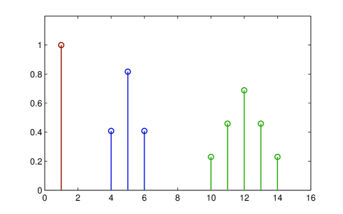
Figure 1: Prototype atoms $\mathbf{p}_{1},\mathbf{p}_{2}$ and $\mathbf{p}_{3}$, which generate the dictionaries $\mathcal{D}_{P_{1}}$, $\mathcal{D}_{P_{2}}$ and $\mathcal{D}_{P3}$ by sequential translations of one point.

Denoting by $\mathcal{D}_{P_{1}}$, $\mathcal{D}_{P_{2}}$ and $\mathcal{D}_{P_{3}}$ the dictionaries arising by translations of the atoms $\mathbf{p}_{1}$, $\mathbf{p}_{2}$, and $\mathbf{p}_{3}$, respectively, the dictionary $\mathcal{D}_{P}$ is built as $\mathcal{D}_{P}=\mathcal{D}_{P_{1}}\cup\mathcal{D}_{P_{2}}\cup\mathcal{D}_{P_{3}}$. The whole dictionary is then built as $\mathcal{D}=\mathcal{D}_{T}\cup\mathcal{D}_{P}$, with $\mathcal{D}_{T}=\mathcal{D}_{C}\cup\mathcal{D}_{S}$. This dictionary was previously introduced as potentially suitable for approximation of GWS [28]. In this study it stands out as being essential for achieving high quality approximation of most of the signals which have been compressed with the proposed codec.

2.3 Coding Strategy

Previously to entropy encoding the coefficients resulting from approximating a signal by partitioning, the real numbers need to be converted into integers. This operation is known as quantization. For all the numerical cases we have adopted a simple uniform quantization technique. The absolute value coefficients $|c_{q}(n)|,\,n=1\ldots,k_{q},\,q=1,\ldots,Q,$ are converted to integers as follows:

$$c^{\Delta}_{q}(n)=\lfloor\frac{|c_{q}(n)|}{\Delta}+\frac{1}{2}\rfloor,$$ (8)

where $\lfloor x\rfloor$ indicates the largest integer number smaller or equal to $x$ and $\Delta$ is the quantization parameter. The signs of the coefficients, represented as $\mathbf{s}_{q},\,q=1,\ldots,Q$, are encoded separately using a binary alphabet.

For creating the stream of numbers to encode the signal model we proceed as in a recent work [27]. The indices of the atoms in the atomic decompositions of each block $\mathbf{f}_{q}$ are first sorted in ascending order $\ell_{i}^{q}\rightarrow\tilde{\ell}_{i}^{q},\,i=1,\ldots,k_{q}$, which guarantees that, for each $q$ value, $\tilde{\ell}_{i}^{q}<\tilde{\ell}_{i+1}^{q},\,i=1,\ldots,k_{q}-1$. This order of the indices induces an order in the unsigned coefficients, $\mathbf{c}^{\Delta}_{q}\rightarrow\mathbf{\tilde{c}}^{\Delta}_{q}$ and in the corresponding signs $\mathbf{s}_{q}\rightarrow\mathbf{\tilde{s}}_{q}$. The ordered indices are stored as smaller positive numbers by taking differences between two consecutive values. By defining $\delta^{q}_{i}=\tilde{\ell}^{q}_{i}-\tilde{\ell}^{q}_{i-1},\,i=2,\ldots,k_{q}$ the follow string stores the indices for block $q$ with unique recovery ${\tilde{\ell}^{q}_{1},\delta^{q}_{2},\ldots,\delta^{q}_{k_{q}}}$. The number ‘0’ is then used to separate the string corresponding to different blocks and entropy code a long string, $st_{\rm{ind}}$, which is built as

$$st_{\rm{ind}}=[{\tilde{\ell}_{1}}^{1},\ldots,\delta^{1}_{k_{1}},0,{\tilde{\ell}_{1}}^{2},\ldots,\delta^{2}_{k_{2}},0,\cdots,{\tilde{\ell}_{1}}^{k_{Q}},\ldots,\delta^{Q}_{k_{Q}}].$$ (9)

The corresponding quantized magnitude of the coefficients are concatenated in the strings $st_{\rm{cf}}$ as follows:

$$st_{\rm{cf}}=[\tilde{c}^{\Delta}_{1}(1),\ldots,\tilde{c}^{\Delta}_{1}(k_{1}),\cdots,\tilde{c}^{\Delta}_{{k_{Q}}}(1),\ldots,\tilde{c}^{\Delta}_{{k_{Q}}}(k_{Q})].$$ (10)

Using ‘0’ to store a positive sign and ‘1’ to store negative one, the signs are placed in the string, $st_{\rm{sg}}$ as

$$st_{\rm{sg}}=[\tilde{s}_{1}(1),\ldots,\tilde{s}_{1}(k_{1}),\cdots,\tilde{s}_{{k_{Q}}}(1),\ldots,\tilde{s}_{{k_{Q}}}(k_{Q})].$$ (11)

The next encoding$/$decoding scheme summarizes the above described procedure.

Encoding

• Given a partition $\mathbf{f}_{q}\in\mathbb{R}^{N_{b}},\,q=1,\ldots,Q$ of a signal, approximate each block $\mathbf{f}_{q}$ by the atomic decompositions (1).

• Quantize, as in (8), the absolute value coefficients to obtain $c_{q}^{\Delta}(n),\,n=1,\ldots,k_{q},\,q=1,\ldots,Q$.

• For each $q$, sort the indices $\ell_{1}^{q},\ldots,\ell_{k_{q}}$ in ascending order to have a new order $\tilde{\ell}_{1}^{q},\ldots,\tilde{\ell}_{k_{q}}$ and the re-ordered sets $\tilde{s}_{q}(1),\ldots,\tilde{s}_{q}(k_{q})$, and $\tilde{c}^{\Delta}_{q}(1),\ldots,\tilde{c}^{\Delta}_{q}(k_{q})$, to create the strings: $st_{\rm{ind}}$, as in (9), and $st_{\rm{cf}}$, and $st_{\rm{sg}}$ as in (10) and (11), respectively. All these strings are encoded, separately, using adaptive arithmetic coding.

Decoding

• Reverse the arithmetic coding to recover strings $st_{\rm{ind}},st_{\rm{cf}},st_{\rm{sg}}$.

• Invert the quantization step as

  $$|\tilde{c}_{q}^{\mathrm{r}}(n)|=\Delta{\tilde{c}}_{q}^{\Delta}(n).$$ (12)

• Recover the approximated partition through the linear combination

  $$\mathbf{f}_{q}^{{\mathrm{r}},k_{q}}=\sum_{n=1}^{k_{q}}\tilde{s}_{q}(n)|{\tilde{c}}_{q}^{\mathrm{r}}(n)|\mathbf{d}_{\tilde{\ell}_{n}^{q}}.$$ (13)

• Assemble the recovered signal as

  $$\mathbf{f}^{\mathrm{r}}=\hat{\operatorname{J}}_{q=1}^{Q}\mathbf{f}_{q}^{{\mathrm{r}},k_{q}}.$$ (14)

3 Results

Given the approximation $\mathbf{f}^{\rm{r}}$ of a signal $\mathbf{f}$, the quality of such an approximation is assessed by the SNR calculated as

$$\text{SNR}=10\log_{10}\frac{\|\mathbf{f}\|^{2}}{\|\mathbf{f}-\mathbf{f}^{\rm{r}}\|^{2}},\quad$$ (15)

where $\|\cdot\|$ indicates the 2-norm.

The local SNR with respect to every block in the partition, which we indicate as $\text{snr}(q),\,q=1,\ldots Q$, is calculated as

$$\text{snr}(q)=10\log_{10}\frac{\|\mathbf{f}_{q}\|^{2}}{\|\mathbf{f}_{q}-\mathbf{f}_{q}^{{\mathrm{r}},k_{q}}\|^{2}},$$ (16)

where $\mathbf{f}_{q}^{{\mathrm{r}},k_{q}}$ is the approximation of the block $\mathbf{f}_{q}$. Both, the mean value ($\overline{\text{snr}}$) and standard deviation (std) of these local quantities are relevant to comparison of point-wise quality recovery. Accordingly, we define

$$\overline{\text{snr}}=\frac{1}{Q}\sum_{q=1}^{Q}\text{snr}(q),\quad\text{and}\quad\text{std}=\sqrt{\frac{1}{Q-1}\sum_{q=1}^{Q}(\text{snr}(q)-\overline{\text{snr}})^{2}}.$$ (17)

In order to use the SNR and $\overline{\text{snr}}$ as measures of quality for comparison, the MP3 signal has to be optimized in relation to those quantities. This is carried out by the following operations[27].

• Shifting: Since MP3 introduces a shift with respect to the original signal, to compute the SNR that shift should be reversed. Denoting by ${\mathbf{f}}_{\mathrm{M}}$ the numerical signal retrieved from the MP3 file, the optimal time shift $\hat{\tau}$ is determined to be the time shift maximizing the cross-correlation with the original signal, i.e.

  $$\hat{\tau}=\operatorname*{arg\,max}_{\tau=-N/2,\ldots,N/2}\,\sum_{n=1}^{N}f(n)f_{\mathrm{M}}(n+\tau).$$ (18)

• Scaling: In order to neutralize the effect of any multiplicative and/or additive constant which could affect the SNR value, we allow for such two constants and adjust them to maximize the SNR as follows: Denoting by $\hat{\mathbf{f}}_{\mathrm{M}}$ the MP3 signal after the shifting operation, we consider the linear form $a\hat{\mathbf{f}}_{\mathrm{M}}+b$ and fix the values of $a$ and $b$ for which $\|\mathbf{f}-(a\hat{\mathbf{f}}_{\mathrm{M}}+b)\|^{2}$ takes the minimum value, i.e.

  $$a = \frac{\langle\mathbf{f},\mathbf{f}_{\mathrm{M}}\rangle-(\frac{1}{N}\sum_{i=1}^{N}\hat{f}_{\mathrm{M}}(i))(\frac{1}{N}\sum_{j=1}^{N}f(j))}{\|\hat{\mathbf{f}}_{\mathrm{M}}\|^{2}-\frac{1}{N}(\sum_{i=1}^{N}f_{\mathrm{M}}(i))^{2}}$$

  $$b = \frac{1}{N}\sum_{i=1}^{N}f(i)-a\frac{1}{N}\sum_{i=1}^{N}\hat{f}_{\mathrm{M}}(i).$$

While the additive constant $b$ is not relevant, the scaling constant $a$ produces an important correction which significantly increases the SNR.

The compression power is determined by the compression ratio (CR) defined as follows

$$\text{CR}=\frac{{\text{Size of the file with the signal}}}{{\text{Size of the compressed file}}}.$$ (19)

In all the numerical examples the files of the signals are given in WAV format. The compression is realized on a single audio channel. The mean value of all the signals is practically zero.

As discussed below, after the shifting and scaling operation for low values of CR (e.g. CR=2 and CR=4) MP3 recovers signals of high quality with respect to both measures, the SNR and the $\overline{\text{snr}}$. The proposed codec, henceforth to be refereed to as ‘dictionary codec’ (DC), is set to produce an approximation of the original signal matching either the SNR or the $\overline{\text{snr}}$ value achieved by the MP3 signal (whatever quantity is the largest one). As seen in the tables below, by matching the largest quantity of either SNR, or $\overline{\text{snr}}$, the other measure is guaranteed to be larger than the value attained by the MP3 signal.

3.1 Numerical Case I

As a first numerical example we consider the audio representation of a detected GW, the chirp gw151226 [29]. This is a short signal, it consists of $N=65536$ points with sampling frequency of 41 kHz. For CR=2 the point-wise quality of the signal recovered from the MP3 file is excellent: SNR=74.6 dB and $\overline{\text{snr}}=70.2$ dB. These values should be appreciated by taking into account that SNR=74.6 dB corresponds to a mean square error between the approximation and the signal of order $10^{-9}$. Since in this case the SNR is greater than the $\overline{\text{snr}}$ the DC is set to produce the same value of SNR. With this restriction the resulting $\overline{\text{snr}}$ is 71.7dB, i.e. larger than the value yielded by MP3. The huge difference between the two encoding procedures is the CR. Denoting by $\mathrm{CR_{\mathrm{M}}}$ the CR with respect to the MP3 file and $\mathrm{CR_{\mathrm{D}}}$ that of the DC file, for SNR=74.6 dB one has $\mathrm{CR_{\mathrm{M}}}=2$ and $\mathrm{CR_{\mathrm{D}}}=23!$ While for larger values of $\mathrm{CR_{\mathrm{M}}}$ the quality of the recovered signal decreases, up to $\mathrm{CR_{\mathrm{M}}}=10$ the quality of the MP3 signal is still very good. Table 1 displays the values of SNR and $\overline{\text{snr}}$, as well as the corresponding CRs produced by both formats. These are differentiated by the notation $\mathrm{SNR}_{\mathrm{M}}$ and $\overline{\mathrm{snr}}_{\mathrm{M}}$, used to indicate the values produced by the MP3 format, and $\mathrm{SNR}_{\mathrm{D}}$ and $\overline{\mathrm{snr}}_{\mathrm{D}}$, used to indicate the values produced by the DC format.

$\mathrm{SNR}_{\mathrm{M}}$	$\mathrm{SNR}_{\mathrm{D}}$	$\overline{\mathrm{snr}}_{\mathrm{M}}$	$\mathrm{std}_{\mathrm{M}}$	$\overline{\mathrm{snr}}_{\mathrm{D}}$	$\mathrm{std}_{\mathrm{D}}$	$\mathrm{CR_{\mathrm{M}}}$	$\mathrm{CR_{\mathrm{D}}}$
74.5 dB	74.5 dB	70.2 dB	6.3	71.7 dB	5.9	2.1	23.2
73.8 dB	73.8 dB	69.8 dB	6.4	71.1 dB	5.7	4.2	24.9
71.3 dB	71.3 dB	66.9 dB	6.7	68.4 dB	5.8	8.4	61.2
69.4 dB	69.4 dB	65.2 dB	6.2	66.4 dB	5.9	10.4	69.3

Table 1: Comparison of $\mathrm{CR_{\mathrm{M}}}$ and $\mathrm{CR_{\mathrm{D}}}$, for the sound representation of the detected chirp gw151226. The first column gives the values of $\mathrm{SNR}_{\mathrm{M}}$ produced by the MP3 signal recovered from files with $\mathrm{CR_{\mathrm{M}}}$ as listed in the 7th column. The second column are the identical values of $\mathrm{SNR}_{\mathrm{D}}$ produced by the signal recovered from the DC files with $\mathrm{CR_{\mathrm{D}}}$ as listed in the last column. The 3rd and 5th columns are the values of $\overline{\mathrm{snr}}_{\mathrm{M}}$ and $\overline{\mathrm{snr}}_{\mathrm{D}}$, respectively. The 4th and 6th columns are the corresponding standard deviations.

3.2 Numerical Case II

In this case the group of GWS has been numerically simulated at MIT [16]. The GWs belong to the EMRI category with circular orbit. The signals are organized in two large subgroups, according to the spin of the larger black hole: spin $99.8\%$ of the maximum value and spin $35.94\%$ of the maximum value. Each subgroup contains 16 signals, each of which is characterized by two angles: the orbital plane and the viewing angle. The signals corresponding to spin $99.8\%$ are listed in the first column Table 2 and Table  3. The signals corresponding to spin $35.94\%$ are listed in the first column of Table 4 and Table 5. The frequency of these signals is 8kHz and were compressed with MP3 at the lowest possible rate, $\mathrm{CR_{\mathrm{M}}}=2$, in the first instance. The recovered signals produce the values of $\overline{\mathrm{snr}}_{\mathrm{M}}$ and $\mathrm{SNR}_{\mathrm{M}}$ given in the second and sixth columns of Table 2. Since in this case $\overline{\mathrm{snr}}_{\mathrm{M}}>\mathrm{SNR}_{\mathrm{M}}$ the DC was set to produce $\overline{\mathrm{snr}}_{\mathrm{D}}=\overline{\mathrm{snr}}_{\mathrm{M}}$. This guarantees that $\mathrm{SNR}_{\mathrm{D}}>\mathrm{SNR}_{\mathrm{M}}$ for all signals. The actual values of $\overline{\mathrm{snr}}_{\mathrm{M}}$ vary with the signals, but for all of them the recovery is of good quality. It corresponds to mean square errors of order of $10^{-8}$. As can be observed in the table, for all the signals the compression performance of the DC format is clearly superior to MP3. Table 3 displays the equivalent results but corresponding to a larger compression ratio of MP3 ($\mathrm{CR_{\mathrm{M}}}=4$).

Signal	$\overline{\mathrm{snr}}_{\mathrm{M}}$	$\mathrm{std}_{\mathrm{M}}$	$\overline{\mathrm{snr}}_{\mathrm{D}}$	$\mathrm{std}_{\mathrm{D}}$	$\mathrm{SNR}_{\mathrm{M}}$	$\mathrm{SNR}_{\mathrm{D}}$	$\mathrm{CR_{\mathrm{M}}}$	$\mathrm{CR_{\mathrm{D}}}$
E1	67.9	2.1	67.9	0.2	65.8	67.8	2	6.8
E2	65.0	2.9	65.0	0.4	58.9	64.9	2	5.3
E3	63.7	3.3	63.7	0.5	54.4	63.6	2	5.2
E4	66.9	3.4	66.9	0.6	55.2	66.7	2	5.6
E5	63.4	1.8	63.4	0.2	62.4	63.4	2	6.0
E6	62.2	2.9	62.3	0.2	58.9	62.1	2	5.1
E7	61.6	2.9	61.6	0.2	57.9	61.6	2	4.9
E8	62.8	2.9	62.8	0.3	59.4	62.8	2	5.2
E9	65.7	2.2	65.7	0.3	64.5	65.7	2	6.4
E10	64.1	2.1	64.1	0.2	62.4	64.1	2	5.6
E11	62.7	1.8	62.7	0.2	62.2	62.7	2	5.5
E12	63.7	2.2	63.7	0.2	63.0	63.7	2	5.8
E13	68.5	4.4	68.5	0.4	64.3	68.5	2	6.3
E14	66.8	2.4	66.8	0.4	65.8	66.8	2	5.6
E15	63.7	2.7	63.7	0.6	62.7	63.6	2	5.7
E16	64.5	2.9	64.5	0.4	62.6	63.7	2	5.9

Table 2: Comparison of $\mathrm{CR_{\mathrm{M}}}$ and $\mathrm{CR_{\mathrm{D}}}$ values for GWs within the EMRI category for circular orbit and spin $99.8\%$ of the maximum value. Each signal listed in the first column corresponds to a particular orbital plane and viewing angle. The second column shows the $\overline{\mathrm{snr}}_{\mathrm{M}}$ values produced by the MP3 signals recovered from a file corresponding to $\mathrm{CR_{\mathrm{M}}}=2$. The sixth column shows the corresponding values of $\mathrm{SNR}_{\mathrm{M}}$. All the other figures in the table arise when setting the DC to achieve $\overline{\mathrm{snr}}_{\mathrm{D}}=\overline{\mathrm{snr}}_{\mathrm{M}}$.

Signal	$\overline{\mathrm{snr}}_{\mathrm{M}}$	$\mathrm{std}_{\mathrm{M}}$	$\overline{\mathrm{snr}}_{\mathrm{D}}$	$\mathrm{std}_{\mathrm{D}}$	$\mathrm{SNR}_{\mathrm{M}}$	$\mathrm{SNR}_{\mathrm{D}}$	$\mathrm{CR_{\mathrm{M}}}$	$\mathrm{CR_{\mathrm{D}}}$
E1	60.3	2.4	60.3	0.3	58.2	60.2	4	9.7
E2	55.5	4.2	55.5	0.4	47.9	55.4	4	7.9
E3	54.1	4.9	54.1	0.4	45.5	54.0	4	7.6
E4	57.5	4.0	57.5	0.6	51.5	57.4	4	8.3
E5	54.9	2.9	54.9	0.2	52.4	54.8	4	8.8
E6	52.4	4.2	52.4	0.2	44.9	52.3	4	7.6
E7	52.2	5.0	52.2	0.2	39.7	52.1	4	7.1
E8	53.6	3.9	53.6	0.3	43.0	53.6	4	7.5
E9	56.5	2.7	56.5	0.2	55.3	56.4	4	9.6
E10	54.7	1.8	54.7	0.2	53.8	54.6	4	8.2
E11	53.2	2.4	53.2	0.2	51.9	53.2	4	8.1
E12	54.4	2.8	54.4	0.2	52.0	54.4	4	8.4
E13	59.4	3.4	59.4	0.4	57.3	59.4	4	8.8
E14	57.4	2.2	57.3	0.3	56.7	57.4	4	7.7
E15	55.5	2.2	55.5	0.3	51.2	55.5	4	7.7
E16	55.0	2.6	55.0	0.5	51.2	55.0	4	8.4

Table 3: Same description as in Table 2 but for $\mathrm{CR_{\mathrm{M}}}=4$.

Table 4 and Table 5 have equivalent description as Table 2 and 3, respectively, but the signals belong to the EMRI group with spin $35.94\%$ of the maximum value.

Signal	$\overline{\mathrm{snr}}_{\mathrm{M}}$	$\mathrm{std}_{\mathrm{M}}$	$\overline{\mathrm{snr}}_{\mathrm{D}}$	$\mathrm{std}_{\mathrm{D}}$	$\mathrm{SNR}_{\mathrm{M}}$	$\mathrm{SNR}_{\mathrm{D}}$	$\mathrm{CR_{\mathrm{M}}}$	$\mathrm{CR_{\mathrm{D}}}$
S1	71.8	3.2	71.8	0.6	68.8	71.7	2	10.2
S2	70.2	2.4	70.2	0.7	67.9	70.1	2	6.6
S3	69.7	2.2	69.7	0.5	67.3	69.6	2	6.4
S4	69.5	2.4	69.5	0.5	67.3	69.4	2	6.4
S5	70.8	2.3	70.8	0.5	68.9	70.8	2	7.7
S6	68.8	1.9	68.8	0.4	67.9	68.7	2	5.5
S7	65.0	3.3	65.0	0.4	61.1	65.0	2	5.4
S8	64.8	1.9	64.8	0.4	63.9	64.7	2	5.8
S9	69.9	2.5	69.9	0.3	68.2	69.9	2	5.2
S10	67.1	1.7	67.1	0.4	66.6	67.2	2	4.6
S11	63.4	2.3	63.4	0.5	62.3	63.5	2	4.5
S12	61.7	2.0	61.7	0.2	60.9	61.7	2	4.5
S13	66.0	3.2	66.0	0.6	62.8	66.1	2	4.9
S14	63.0	7.2	63.0	1.6	61.6	64.4	2	4.9
S15	59.0	8.4	59.0	1.3	59.5	60.2	2	4.9
S16	51.8	2.0	51.8	0.3	51.0	51.9	2	4.7

Table 4: Same description as for Table 2 but the signals belong to the EMRI group with spin $35.94\%$ of the maximum value.

Signal	$\overline{\mathrm{snr}}_{\mathrm{M}}$	$\mathrm{std}_{\mathrm{M}}$	$\overline{\mathrm{snr}}_{\mathrm{D}}$	$\mathrm{std}_{\mathrm{D}}$	$\mathrm{SNR}_{\mathrm{M}}$	$\mathrm{SNR}_{\mathrm{D}}$	$\mathrm{CR_{\mathrm{M}}}$	$\mathrm{CR_{\mathrm{D}}}$
S1	66.3	3.2	66.3	0.5	61.9	66.4	4	13.1
S2	62.9	2.7	62.9	0.5	58.7	62.8	4	9.2
S3	61.4	2.9	61.4	0.5	57.5	61.2	4	9.3
S4	61.6	2.4	61.6	0.5	58.6	61.5	4	9.0
S5	64.1	2.9	64.1	0.5	61.3	64.0	4	10.3
S6	61.1	2.1	61.1	0.4	59.2	61.0	4	7.9
S7	57.3	2.5	57.3	0.4	54.8	57.3	4	7.8
S8	56.8	2.5	56.8	0.4	54.5	56.8	4	8.3
S9	61.3	2.6	61.3	0.3	59.9	61.2	4	8.0
S10	58.1	2.2	58.1	0.4	56.7	58.1	4	7.2
S11	54.2	2.6	54.2	0.5	52.9	54.3	4	7.1
S12	53.8	2.0	53.8	0.2	53.0	53.8	4	6.8
S13	56.8	2.9	56.8	0.6	54.4	56.8	4	7.7
S14	55.1	7.4	55.1	1.2	54.0	56.1	4	7.0
S15	51.0	7.5	51.0	1.2	51.7	52.0	4	7.0
S16	44.7	2.7	44.7	0.7	43.1	44.6	4	6.6

Table 5: Same as the description of Table 4 but for $\mathrm{CR_{\mathrm{M}}}=4$.

3.3 Numerical Case III

This group of signals has also been simulated at MIT. All the signals belong to the Binary category, for circular systems, and are differentiated by the mass of the larger body. The first two signals listed in Tables 6 and 7 correspond to bodies of roughly the same mass. The first signal (B1) is generated by binary neutron stars each of 1.5 solar masses. The second signal (B2) is generated by binary black holes, each of 2.5 solar masses. Signals B3 and B4 are produced by binary black holes with mass ratio 3:1. The signal B3 does not include spin effects while B4 includes rapid spinning of both bodies.

The minimum possible values of $\mathrm{CR_{\mathrm{M}}}$ are given in the eighth column of Table 6. In this case $\mathrm{SNR}_{\mathrm{M}}>\overline{\mathrm{snr}}_{\mathrm{M}}$ for all the signals. Hence, the DC was set to achieve $\mathrm{SNR}_{\mathrm{M}}=\mathrm{SNR}_{\mathrm{D}}$ (second and third columns of Table 6). These values produced $\overline{\mathrm{snr}}_{\mathrm{D}}>\overline{\mathrm{snr}}_{\mathrm{M}}$ for all the signals. The remarkable performance of the DC emerges from the $\mathrm{CR_{\mathrm{D}}}$ figures listed in the last column of Table 6.

Signal	$\mathrm{SNR}_{\mathrm{M}}$	$\mathrm{SNR}_{\mathrm{D}}$	$\overline{\mathrm{snr}}_{\mathrm{M}}$	$\mathrm{std}_{\mathrm{M}}$	$\overline{\mathrm{snr}}_{\mathrm{D}}$	$\mathrm{std}_{\mathrm{D}}$	$\mathrm{CR_{\mathrm{M}}}$	$\mathrm{CR_{\mathrm{D}}}$
B1	70.2	70.2	66.2	8.5	67.2	8.0	2.7	51.7
B2	70.3	70.3	65.2	10.4	66.5	9.5	2.6	34.2
B3	59.0	59.0	58.5	2.0	58.8	0.6	2.7	29.3
B4	55.6	55.6	54.9	2.1	55.2	0.7	2.7	28.9

Table 6: Comparison of the $\mathrm{CR_{\mathrm{M}}}$ and $\mathrm{CR_{\mathrm{D}}}$ values for the audible part of the signals in the Binary group. The second column gives the values of $\mathrm{SNR}_{\mathrm{M}}$ produced by the MP3 signal recovered from files with $\mathrm{CR_{\mathrm{M}}}$ as listed the 8th column. The 3rd column are the identical values of $\mathrm{SNR}_{\mathrm{D}}$ produced by the signal recovered from the DC files with $\mathrm{CR_{\mathrm{D}}}$ as listed in the last column. The 4th and 6th columns are the values of $\overline{\mathrm{snr}}_{\mathrm{M}}$ and $\overline{\mathrm{snr}}_{\mathrm{D}}$, respectively. The 5th and 7th columns are the corresponding standard deviations.

Signal	$\mathrm{SNR}_{\mathrm{M}}$	$\mathrm{SNR}_{\mathrm{D}}$	$\overline{\mathrm{snr}}_{\mathrm{M}}$	$\mathrm{std}_{\mathrm{M}}$	$\overline{\mathrm{snr}}_{\mathrm{D}}$	$\mathrm{std}_{\mathrm{D}}$	$\mathrm{CR_{\mathrm{M}}}$	$\mathrm{CR_{\mathrm{D}}}$
B1	68.8	68.8	65.9	8.6	65.9	7.8	5.4	56.2
B2	68.6	68.6	65.0	10.5	65.0	9.4	5.2	36.9
B3	53.4	54.1	53.9	2.9	53.9	0.4	5.5	37.5
B4	49.3	49.6	49.7	3.4	49.7	0.4	5.5	39.3

Table 7: Same description as Table 6 but for double values of $\mathrm{CR_{\mathrm{M}}}$.

4 Discussion

The results of Tables 1-7 demonstrate the remarkable compression power of the DC, in comparison to MP3 at equivalent high quality of the recovered signal. For all cases the relation

$$\mathrm{CR_{\mathrm{D}}}=\gamma\,\,\mathrm{CR_{\mathrm{M}}}$$ (20)

holds for values of $\gamma$ varying from a minimum value $\gamma_{\min}=1.7$ for signal S12 in Table 5 to a maximum value $\gamma_{\max}=19.2$ for signal B1 in Table 6. Table 8 shows the mean value $\bar{\gamma}$ in each of the above tables. It also shows the corresponding $\mathrm{std}$ as well as the values of $\gamma_{\min}$ and $\gamma_{\max}$ in each of the tables.

Table	$\bar{\gamma}$	$\mathrm{std}$	$\gamma_{\min}$	$\gamma_{\max}$
1	7.7	2.3	5.9	11.0
2	2.8	0.3	2.4	3.4
3	2.1	0.2	1.8	2.4
4	2.9	0.7	2.2	5.1
5	2.2	0.6	1.7	3.2
6	13.5	3.9	10.8	19.2
7	7.7	1.4	6.8	9.7

Table 8: Statistic of the factor $\gamma$ (c.f. (20)) for Table 1-7. The second column corresponds to the mean value with respect to the signals in each table. The third column gives the corresponding standard deviation.

It is worth commenting that the component of the dictionary containing the atoms of small support plays an essential role of achieving large values of $\mathrm{CR_{\mathrm{D}}}$ for high quality recovery. This is much more important for the group of EMRI sound. For example, if the compression of signal E1 in Table 2 is carried out in the same way but excluding the sub-dictionary with those atoms, the value of $\mathrm{CR_{\mathrm{D}}}$ drops from 6.8 to 3.5. Nevertheless, even if for approximating E1 at the quality of Table 2 the percentage of atoms of small support is significant ($41\%$) the contribution to the signal approximation is minor. The norm of the signal E1 is 207.6 and the norm of component generated by the atoms of small support is only 2.1. This component of small norm is needed to achieve the high values of $\overline{\mathrm{snr}}_{\mathrm{D}}$ and $\mathrm{SNR}_{\mathrm{D}}$ required in this study. Contrarily, for compression of lower quality recovery these atoms play no role for most signals. At lower quality, however, the power of the DC increases substantially. For example, when compressing with MP3 and $\mathrm{CR_{\mathrm{M}}}=8$ the signal E1 the recovered signal produces $\overline{\mathrm{snr}}_{\mathrm{M}}=41.3$ dB. The DC achieves the same value of $\overline{\mathrm{snr}}_{\mathrm{D}}$ (and $\mathrm{SNR}_{\mathrm{D}}>\mathrm{SNR}_{\mathrm{M}}$) for $\mathrm{CR_{\mathrm{D}}}=53!$

4.1 Beyond Compression

The success of the DC in producing a small file stems from the ability of constructing a signal approximation of good quality, but involving less elementary components than the number of samples giving the signal. Let’s suppose that to represent at the desired quality the block $\mathbf{f}_{q}$ in the signal partition one needs $k_{q}$ dictionary atoms, and let’s normalize these values $\tilde{k}_{q}={k_{q}}/\sum_{q=1}^{Q}{k_{q}}$ for comparison purposes. As shown in Fig. 2 the numbers $\tilde{k}_{q},\,q=1,\ldots,Q$ render meaningful information about the signal internal variations over time. In the lower graphs of Fig. 2 each of these values is located in the horizontal axis at the center of the corresponding block (of size $N_{b}=2048$) and provides a condensed digital summary of the sound. The left upper graph is the spectrograms of the signal E1. The lines in the lower left graph join the values $\tilde{k}_{q},\,q=1,\ldots,225$ resulting when approximating this signal at three different qualities: $\overline{\mathrm{snr}}_{\mathrm{D}}=65$, 60 and 55 dB. As observed in the graph, the three lines are very close to each other and account for the node in the spectrogram which occurs at around 55 secs. The right upper graph of Fig.2 is the spectrogram of the signal S1. This signal differs from the signal E1 only in the spin ($35.94\%$ of the maximum value). Also in this case, the three lines connecting the values $\tilde{k}_{q},\,q=1,\ldots,66$ for approximations of $\overline{\mathrm{snr}}_{\mathrm{D}}=65$, 60, and 55 dB are close to each other and account for the main feature of the spectrogram, which is characterized by a rise of frequency towards the end. It is an interesting feature of the digital summary, given by the points in the lower graphs, the small cardinality in relation to the length of the signal: 225 points for the signal E1 given by $N=460800$ samples and 66 points for the signal S1 given by $N=135168$ samples.

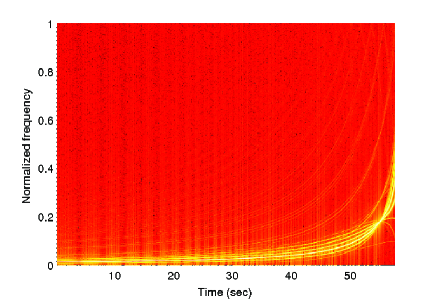
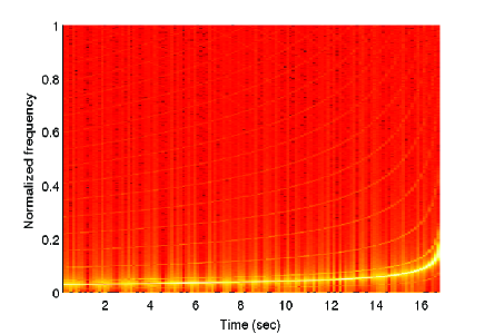
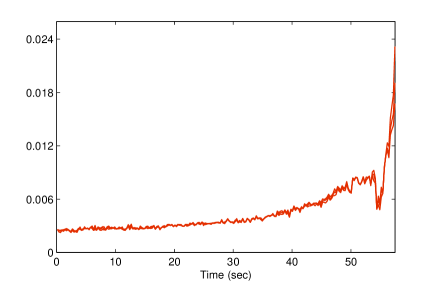
Figure 2: The upper graphs are the spectrograms of the signals E1 (left) and S1 (right). The lines in the lower graphs join the values $\tilde{k}_{q}=1,\ldots,Q$ resulting when approximating these signals at three different qualities: $\overline{\mathrm{snr}}_{\mathrm{D}}=65$, 60, and 55 dB. In the left graph each of the three lines joins $Q=225$ points. In the right graph $Q=66$ points.

5 Conclusions

A dedicated codec for compression of gravitational sound with high quality recovery has been proposed. The power of the format to store this type of sound stems from the mathematical model for representing the signal. The model is based on recursive selection of elementary components approximating the signal with accuracy. The components, called atoms, are chosen from a redundant set, called a dictionary, which is the union of two sub-dictionaries consisting of atoms of different nature. One sub-dictionary contains trigonometric atoms. The other sub-dictionary contains pulses of small support. While the contribution of the atoms of small support to the signal approximation is minor, they are necessary to obtain approximations of high accuracy. At lower quality recovery (less than 50 dB) this sub-dictionary could be avoided and the compression power of the proposed codec would be even more potent. Nonetheless, the study reported here focuses on compression with high quality point-wise recovery.

The proposal was tested on the sound representation of the detected short chirp gw151226, and on a set of longer signals numerically simulated at MIT. Comparisons with the compression standard MP3 resulted in a significant increment of compression power for equivalent quality of the recovered signal. As a byproduct, the codec generates a condensed digital summary of the sound which could be of assistance for identification tasks.

Note: All the results in this paper can be reproduced using the MATLAB software which has been made available on [32].

References

- [1] B. P. Abbott et al. (LIGO Scientific Collaboration and Virgo Collaboration), “Observation of Gravitational Waves from a Binary Black Hole Merger”, Phys. Rev. Lett. 116, 061102 (2016), DOI: 10.1103/PhysRevLett.116.061102
- [2] B. P. Abbott et al. (LIGO Scientific Collaboration and Virgo Collaboration), “GW151226: Observation of Gravitational Waves from a 22-Solar-Mass Binary Black Hole Coalescence” , Phys. Rev. Lett., 116, 2411003 (2016) DOI 10.1103/PhysRevLett.116.241103.
- [3] B. P. Abbott et al. (LIGO Scientific Collaboration and Virgo Collaboration), “GW170104: Observation of a 50-Solar-Mass Binary Black Hole Coalescence at Redshift 0.2”, Phys. Rev. Lett., 118, 221101 (2017) DOI:10.1103/PhysRevLett.118.221101.
- [4] B. P. Abbott et al. (LIGO Scientific Collaboration and Virgo Collaboration),“GW170814: A three-detector observation of gravitational waves from a binary black hole coalescence”, Phys. Rev. Lett., 119, 141101 (2017) DOI:10.1103/PhysRevLett.119.141101.
- [5] B. P. Abbott et al. (LIGO Scientific Collaboration and Virgo Collaboration), “GW170608: Observation of a 19-solar-mass Binary Black Hole Coalescence”, The Astrophysical Journal Letters, 851, 2 (2017).
- [6] B. P. Abbott et al. (LIGO Scientific Collaboration and Virgo Collaboration),“GW170817: Observation of Gravitational Waves from a Binary Neutron Star Inspiral”, Phys. Rev. Lett., 119, 161101 (2017). DOI:10.1103/PhysRevLett.119.161101.
- [7] F. Pretorius, “Evolution of Binary Black-Hole Spacetimes”. Phys. Rev. Lett. 95 121101 (2015). doi:10.1103/PhysRevLett.95.121101.
- [8] M. Campanelli, C. O. Lousto, P. Marronetti, Y. Zlochower, “Accurate Evolutions of Orbiting Black-Hole Binaries without Excision”, Phys. Rev. Lett. 96 111101 (2006) doi:10.1103/PhysRevLett.96.111101.
- [9] J. G. Baker, J. Centrella, D-Il Choi, M. Koppitz, J. van Meter, (2006). “Gravitational-Wave Extraction from an Inspiraling Configuration of Merging Black Holes”.Phys. Rev. Lett., 96 111102. doi:10.1103/PhysRevLett.96.111102.
- [10] L. Blanchet, Living Rev. Relativ. (2014) 17: 2. https://doi.org/10.12942/lrr-2014-2
- [11] S. A. Hughes, “The evolution of circular, non-equatorial orbits of Kerr black holes due to gravitational-wave emission”, Phys. Rev. D, 61, 084004 (2000).
- [12] S. A. Hughes, “Evolution of circular, non-equatorial orbits of Kerr black holes due to gravitational-wave emission: II. Inspiral trajectories and gravitational waveforms”, Phys. Rev. D, 64, 064004 (2001).
- [13] K. Glampedakis, S. A. Hughes, D. Kennefick, “Approximating the inspiral of test bodies into Kerr black holes”, Phys. Rev. D, 66, 064005 (2002).
- [14] S. A. Hughes, S. Drasco, E. E. Flanagan, J. Franklin, “Gravitational radiation reaction and inspiral waveforms in the adiabatic limit, Phys. Rev. Lett. 94, 221101 (2005).
- [15] S. Drasco and S. A. Hughes, “Gravitational wave snapshots of generic extreme mass ratio inspirals”, Phys. Rev. D, 73, (2006).
- [16] http://gmunu.mit.edu/sounds
- [17] E. Ravelli, G. Richard and L. Daudet, “Union of MDCT bases for audio coding”, IEEE Transactions on Audio, Speech, and Language Processing, 1361–1372 (2008).
- [18] H. Lee, P. Pham, Y. Largman, and AY Ng, “Unsupervised feature learning for audio classification using convolutional deep belief networks”, Advances in Neural Information Processing Systems 22, 1096–1104 (2009).
- [19] M. D. Plumbley, T. Blumensath, L. Daudet, R. Gribonval, and M. E. Davies, “Sparse representations in audio and music: From coding to source separation,” Proc. IEEE, 98, 995–1005 (2010).
- [20] J. Nam, J. Herrera, M. Slaney, and J. Smith, “Learning sparse feature representations for music annotation and retrieval,” in Proceedings of the 13 International Society for Music Information Retrieval Conference, 565–5870 (2012).
- [21] H. Henaff , K. Jarrett , K. Kavukcuoglu , and Y. LeCun , “Unsupervised learning of sparse features for scalable audio classification,” in Proceedings of the 15th International Society for Music Information Retrieval Conference (2014), pp. 77–82.
- [22] L. F. Yu , L. Su , and Y. H. Yang , “Sparse cepstral codes and power scale for instrument identification”, in Proceedings of IEEE International Conference on Acoustics, Speech and Signal Processing (2014), pp. 7460–7464.
- [23] Y. Vaizman, B. McFee, and G. Lanckriet, “Codebook-based audio feature representation for music information retrieval”, IEEE/ACM Transactions on Audio, Speech and Language Processing, 22, 1483–1493 (2014).
- [24] M. Panteli, E. Benetos and S. Dixon (2016), Learning a Feature Space for World Music Style Similarity. 17th International Society for Music Information Retrieval Conference (ISMIR 2016), pp 538-544).
- [25] Y. Han, S. Lee, J. Nam, and K. Lee, “Sparse feature learning for instrument identification: Effects of sampling and pooling methods”, The Journal of the Acoustical Society of America 139, 2290–2298 (2016).
- [26] L. Rebollo-Neira and G. Aggarwal, “A dedicated greedy pursuit algorithm for sparse spectral modelling of music sound”, Journal of The Acoustic Society of America, 140, 2933–2943 (2016).
- [27] L. Rebollo-Neira and I. Sanches, , “Simple scheme for compressing sparse representation of melodic music”, Electronics Letters (2017) DOI:10.1049/el.2017.3908
- [28] L. Rebollo-Neira and A. Plastino, “Sparse representation of Gravitational Sound”,Journal of Sound and Vibration, 417, 306–314 (2017) DOI:10.1016/j.jsv.2017.12.007
- [29] http://www.ligo.org/multimedia
- [30] L. Rebollo-Neira and D. Lowe, “Optimized orthogonal matching pursuit approach”, IEEE Signal Process. Letters, 9, 137–140 (2002).
- [31] L. Rebollo-Neira, “Cooperative greedy pursuit strategies for sparse signal representation by partitioning”, Signal Processing, 125, 365–375 (2016).
- [32] http://www.nonlinear-approx.info/examples/node010.html
- [33] http://www.ux.uis.no/karlsk/proj99