Probing Heavy Charged Higgs Boson at the LHC

Abstract

Signature of heavier charged Higgs boson, much above the top quark mass, is investigated at the LHC Run 2 experiments, following its decay mode via top and bottom quark focusing on both hadronic and semi-leptonic signal final states. The generic two Higgs doublet model framework is considered with a special emphasis on supersymmetry motivated Type II model. The signal is found to be heavily affected by huge irreducible backgrounds due to the top quark pair production and QCD events. The jet substructure technique is used to tag moderately boosted top jets in order to reconstruct charged Higgs mass. The simple cut based analysis is performed optimizing various kinematic selections, and the signal sensitivity is found to be reasonable for only lower range of charged Higgs masses corresponding to 3000 fb^-1 integrated luminosity. However, employing the multi-variate analysis(MVA) technique, a remarkable improvement in signal sensitivity is achieved. We find that the charged Higgs signal for the mass range about $300-600$ GeV is observable with 1000 $\text{fb}^{-1}$ luminosity. However, for high luminosity, ${\cal L}=3000\text{fb}^{-1}$, the discovery potential can be extended to $700-800$ GeV.

1 Introduction

The recent discovery of the 125 GeV Higgs boson [1, 2] at the CERN Large Hadron collider (LHC) provides the last missing piece of the Standard Model (SM), and open up a new window to explore the physics beyond standard model(BSM). Although, the current precision measurements of various properties of the Higgs boson, in particular the couplings with fermions and gauge bosons, indicate that it is indeed the candidate for the SM Higgs [3], nonetheless, it does not rule out many BSM scenario. Among the plethora of BSM candidates. The supersymmetry based models, such as minimal supersymmetric standard model(MSSM) is the most popular and very well studied BSM scenario, it provides elegant solutions to some of the short comings of the SM, and predicts rich and diverse phenomenology to be testable directly in colliders.

Recall, the MSSM requires at least two Higgs doublets to make the theory anomaly free, and also to generate the masses of up and down type of fermions. The theories with extended Higgs sector predict more Higgs boson - neutral and charged states. In general, two Higgs doublet model(2HDM) consisting of an extra SU(2) Higgs doublet added with the SM Higgs doublet, is well motivated and consistent with the Higgs discovery. In fact, the 2HDM can be interpreted as the effective theory at low energy of many BSM theories with UV completion. For example, the Higgs sector in supersymmetric model may appear as a simple 2HDM (Type II), if the masses of all sparticles decouple at a very high scale. Generally, 2HDM is classified into four categories, Type I, II, III and IV depending on the nature of Yukawa couplings, subject to $Z_{2}$ symmetry in order to avoid Flavor changing neutral current (For more details about 2HDM, see Ref. [4] and  [5]). In all classes of 2HDM scenario, there exist five physical Higgs boson states, two CP even ($h,H$, with the assumption, $m_{h}<m_{H}$), one CP odd ($A$), and two charged Higgs bosons(${H}^{\pm}$). The lightest CP even Higgs $h$ can be interpreted as the SM-like Higgs boson in the decoupling limit, where the other states turn out to be very heavy, much above the electroweak scale [6]. However, some other studies also show that CP even Higgs states may behave as SM-like with mass 125 GeV in the alignment limit even without decoupling [7, 8, 9, 10]. Presence of extra physical Higgs boson states along with the SM-like Higgs is one of the characteristics of BSM. Needless to say, discovery of an extra Higgs boson certainly confirms the existence of BSM. Therefore, looking for these additional Higgs bosons in various decay channels over a wide range of masses is a top priority program in the current LHC experiment.

In this context, searching for the charged Higgs boson signal is unique, since discovery of it clearly, and unambiguously confirms the presence of BSM. Therefore, the study of charged Higgs boson has received special attention both phenomenologically and experimentally. For the lower mass range, less than the top quark mass, $m_{{H}^{\pm}}<m_{t}$, the phenomenology of the charged Higgs boson is well studied, and also experimentally probed thoroughly in many of its decay channels. However, detection of the charged Higgs boson for the heavier mass range, greater than the top quark mass($m_{{H}^{\pm}}\gg m_{t}$), is found to be very challenging due to huge contamination by the irreducible SM backgrounds. In this current study, we attempt to find the discovery potential of the charged Higgs boson for this heavier mass range ($m_{{H}^{\pm}}\gg m_{t}$). The study is carried out within the framework of the generic 2HDM with an emphasis on Type II 2HDM motivated by supersymmetry. The charged Higgs boson couplings with fermions are strongly dependent on $\tan\beta$, and hence its production and subsequent decays sensitive to $\tan\beta$. In hadron colliders, in the lower mass range $\left({m_{{H}^{\pm}}}<m_{t}\right)$, the charged Higgs bosons are produced via a pair production of top quark, $p\bar{p}$/$pp\to t\bar{t}$ following the decay ${t}\rightarrow{{H}^{+}}{b}$. For intermediate and heavier mass range, it is mainly produced directly in association with a top quark(and also a $b$ quark) [11]. Furthermore, charged Higgs boson can be produced in SUSY cascade decays via heavier chargino and neutralino production in gluino and squark decays [12, 13].

So far, non observation of any charged Higgs signal events in direct searches constrain its production and decay in a model independent way, which in turn can be translated to exclude the relevant parameter space, in particular $\tan\beta$ and $m_{{H}^{\pm}}$, for a given model framework. For example, in the past, direct searches at LEP [14] and Tevatron [15] experiments excluded lower mass range of $m_{{H}^{\pm}}$ in terms of $\tan\beta$. At the LHC Run 1 experiments with $\sqrt{s}=7$ and 8 TeV data, lighter charged Higgs boson is probed in the decay channels $\tau\nu$ [16, 17], $cs$ [18, 19] and also $cb$[20], while at Run 2 with $\sqrt{s}=13$ TeV energy, mainly the decay modes $\tau\nu$ [21, 22], and $tb$ [23] are considered to probe it upto $\sim 1$ TeV mass. The absence of any signal event in ${{{H}^{+}}\rightarrow{\tau}^{+}\nu_{\tau}}$ decay modes in CMS at 13 TeV energy with an integrated luminosity 12.9 $\text{fb}^{-1}$ leads an exclusion of the cross section times respective branching ratio for the mass range $180\text{ GeV}<m_{{H}^{\pm}}<3\text{ TeV}$, where as limits on the ${\text{Br}\left({{t}\rightarrow{{H}^{+}}{b}}\right)}\times{\text{Br}\left({{{H}^{+}}\rightarrow{\tau}^{+}\nu_{\tau}}\right)}$ are set for the range $80\text{ GeV}<m_{{H}^{\pm}}<160\text{ GeV}$ [21]. Eventually, these exclusion limits, rule out $m_{{H}^{\pm}}\sim 90-160$ GeV corresponding to the entire range of $\tan\beta$ up to 60 in the context of MSSM with $m_{h}^{mod+}$ scenario [24], except a hole around $m_{{H}^{\pm}}\sim 150-160$, and $\tan\beta\sim 10$. Similar results are also published from ATLAS [22] at $\sqrt{s}=13$ TeV. The searches in the ${{H}^{+}}\rightarrow{t}\bar{b}$ decay channel for heavier mass range carried out by ATLAS at $\sqrt{s}=13$ TeV and ${\cal L}=13.2$ fb^-1 excluded $m_{{H}^{\pm}}\sim 300-900$ GeV for a very low $\tan\beta\left(\sim 0.5-1.7\right)$ region [23], where as for high values of $\tan\beta>44(60)$, $m_{{H}^{\pm}}\sim 300$(366)GeV are excluded. Note that this decay channel is also probed at $\sqrt{s}=8$ TeV by ATLAS including the s-channel charged Higgs production, and exclusion are presented for the cross section times Br$\left({{H}^{+}}\rightarrow{t}\bar{b}\right)$[25]. However these limits are found to be very weak in comparison to the predictions from ${{H}^{+}}\rightarrow{\tau}^{+}\nu_{\tau}$ searches [16, 22]. Remarkably, the most stringent constraints on the charged Higgs sector in the context of SUSY motivated Type II type of model are predicted indirectly by the neutral Higgs boson searches, $pp\to{h},{H},{A}\to\tau\bar{\tau}$ at the LHC [26]. It can be attributed to the fact that the neutral Higgs boson couplings with tau leptons very strongly depends on $\tan\beta$, in particular for higher values of it. Exclusion region predicted by these neutral Higgs boson searches, imply a limit on $\tan\beta>6$ for $m_{A}<250$ GeV, where as Higher values of $\tan\beta$($>20$ are completely ruled out up to 60, for $m_{A}\sim m_{{H}^{\pm}}\sim 1000$ GeV, $m_{A}$ is the mass of the pseudoscalar Higgs, related with the charged Higgs mass as, $m_{{H}^{\pm}}^{2}=m_{W}^{2}+m_{A}^{2}$ in SUSY model (like Type II model). In addition to these direct limits, the charged Higgs sector is also constrained by flavor physics data. Strong contribution via loops to the Br of rare decay modes of B meson makes it very sensitive to flavor physics observables. Measurements of these Br by B-factories, and also at the LHC and LHCb put very strong limit to the charged Higgs sector. More details about these latest constraints in the framework of 2HDM can be found in a recent review of Ref. [27], and references therein.

In the phenomenological side, there have been numerous studies on exploring the ${H}^{\pm}$ signal in various decay channels in the context of the MSSM Higgs sector [28, 29, 30, 31, 32, 33, 34, 35, 36, 37, 38], and as well as in 2HDM framework [39, 30, 40, 41] using various interesting techniques. More details about charged Higgs phenomenology can be found in Ref. [42]. It is worth to mention here about the use of $\tau$ lepton polarization in its 1 and 3 prong decay for ${{H}^{+}}\rightarrow{\tau}^{+}\nu_{\tau}$, which is found to be very useful in extracting the signal suppressing $t\bar{t}$ and QCD background [43, 44, 45]. The signal of charged Higgs boson is also probed in the subdominant production channels ${{H}^{\pm}}W^{\mp}$ [46] and ${H}^{+}{H}^{-}$ [47, 48]. Discovery potential of charged Higgs for heavier mass (${m_{{H}^{\pm}}}>m_{t}$) range with its dominant decay mode ${{H}^{+}}\rightarrow{t}\bar{b}$ is investigated by many authors in the framework of SUSY models [49, 50, 51, 52]. For instance, in the Ref.[52], authors used triple and four b-tagging in order to suppress SM background, which also costs signal significantly as well. Consequently, for heavier mass range, it is found to be very hard to achieve a reasonable signal sensitivity, due to large $t\bar{t}$ and QCD backgrounds. A recent study [53] reports about the detection prospect of charged Higgs signal for heavier mass $\gtrsim 1$ TeV applying jet substructure technique to tag top quarks from the charged Higgs decay in the framework of 2HDM. The authors predicted reasonable sensitivities of charged Higgs signal around the mass of 1 TeV, and found difficult to probe it for the intermediate mass range. The jet substructure technique is also used to look for heavy charged Higgs boson signal in the decay channel ${H}^{\pm}\to W^{\pm}A$ for lighter $A$ boson states[54, 55]. In this current study, we explore the detection prospect of charged Higgs boson for the intermediate to heavier mass range, $300-1000$ GeV, considering the decay mode, ${{H}^{+}}\rightarrow{t}\bar{b}$ with the hadronic and leptonic final state. For heavier mass of ${H}^{\pm}$, the top quark from its decay is expected to be boosted, and we try to exploit this feature by employing the technique of jet substructures to reconstruct the top quark, and subsequently the charged Higgs boson. This method helps to avoid the combinatorial problem while reconstructing the top quark simply by combining the hard jets. In this study, first we attempt to obtain signal sensitivity using cut based analysis, and then try to improve the sensitivity employing the multivariate(MVA) analysis. Performing a detail analysis in the MVA framework, we achieve a remarkable improvements in signal sensitivity, and results are presented for three integrated luminosity options ${\cal L}=300$ $\text{fb}^{-1}$, 1000 $\text{fb}^{-1}$ and 3000 $\text{fb}^{-1}$. Finally, for the sake of completeness, signal sensitivities are predicted for all classes of 2HDM corresponding to a few benchmark parameter space.

We present this study as follows. Briefly describing the 2HDM in Sec.2, the charged Higgs production is discussed in Sec.3. In Sec.4, the signal and backgrounds are discussed, and subsequently, details of simulation are presented in the subsection 4.2 with a brief description about top tagging in subsection 4.1. The results based on cut and count analysis are discussed in subsection 4.3, while in Sec.5 the results based on MVA analysis are presented. Finally we summarize in Sec.6.

2 Two Higgs doublet Model

In the context of our present study, it is instructive to discuss very briefly about the 2HDM. In this model, an extra SU(2) Higgs doublet is added with the SM Higgs doublet. The most general 2HDM potential consisting two doublets $\phi_{1}$ and $\phi_{2}$ with hypercharge Y=+1 is given by [4, 5],

$$V = m_{11}^{2}\phi_{1}^{2}+m_{22}^{2}\phi_{2}^{2}-m_{12}^{2}(\phi_{1}^{\dagger}\phi_{2}+\phi_{1}\phi_{2}^{\dagger})$$ (2.1)

$$+ \frac{\lambda_{1}}{2}(\phi_{1}^{\dagger}\phi_{1})^{2}+\frac{\lambda_{2}}{2}(\phi_{2}^{\dagger}\phi_{2})^{2}+\lambda_{3}(\phi_{1}^{\dagger}\phi_{1})(\phi_{2}^{\dagger}\phi_{2})$$

$$+ \lambda_{4}(\phi_{1}^{\dagger}\phi_{2})(\phi_{2}^{\dagger}\phi_{1})+\frac{\lambda_{5}}{2}\left[\left(\phi_{1}^{\dagger}\phi_{2})^{2}+(\phi_{2}^{\dagger}\phi_{1})^{2}\right)\right]$$

For simplifications, all the free parameters are assumed to be real to conserve CP property, and the discrete $Z_{2}$ symmetry, $\phi_{1}\to-\phi_{1}$ and $\phi_{2}\to+\phi_{2}$ is imposed to suppress FCNC at the tree level. The $Z_{2}$ symmetry is softly broken by the terms proportional to $m_{12}$. The minimum of the potential $V$ is ensured by two vacuum expectation values(vevs), which break the symmetry down to U(1)${}_{\text{em}}$ symmetry,

$$<\phi_{1}>=\left[{\begin{array}[]{c}0\\ \frac{v_{1}}{\sqrt{2}}\\ \end{array}}\right],<\phi_{2}>=\left[{\begin{array}[]{c}0\\ \frac{v_{2}}{\sqrt{2}}\\ \end{array}}\right]$$ (2.6)

where $v_{1}$ and $v_{2}$ are two vevs corresponding to neutral components of $\phi_{1}$ and $\phi_{2}$ respectively, with $v=\sqrt{v_{1}^{2}+v_{2}^{2}}$. The ratio of two vevs defined to be $\tan\beta=\frac{v_{2}}{v_{1}}$ is considered as one of the free parameter of the model. Expanding the doublets around the minimum of the potential, the Higgs fields can be given by[4, 5],

$$\phi_{1}=\left({\begin{array}[]{c}\phi_{1}^{+}\\ \frac{1}{\sqrt{2}}(v\cos\beta+\phi_{1}^{0})\\ \end{array}}\right),\phi_{2}=\left({\begin{array}[]{c}\phi_{2}^{+}\\ \frac{1}{\sqrt{2}}(v\sin\beta+\phi_{2}^{0}).\\ \end{array}}\right)$$ (2.11)

Already mentioned in the previous section that after symmetry breaking, the potential predicts five physical Higgs boson states, two neutral CP even states, $h$ and $H$($m_{h}<m_{H}$), one neutral CP odd state A, and two charged states ${H}^{\pm}$. The physical charged state and CP odd neutral states are expressed as,

$${{H}^{\pm}}=-\phi_{1}^{\pm}\sin\beta+\phi_{2}^{\pm}\cos\beta,$$ (2.12)

$$A=\sqrt{2}\left(-\text{Im}\phi_{1}^{0}\sin\beta+\text{Im}\phi_{2}^{0}\cos\beta\right).$$ (2.13)

The two CP even neutral weak states mix through an angle $\alpha$ providing two mass eigenstates, $h$ and $H$. The input parameters present in the potential V, can be re-expressed in terms of physical masses and other parameters such as,

$$m_{h},m_{H},m_{A},{m_{{H}^{\pm}}},\tan\beta,\sin(\beta-\alpha),v,m_{12}^{2}.$$ (2.14)

Note that $v$ is set to be at the electroweak scale ($=246$ GeV), and one of the CP even Higgs boson can be interpreted as the recently discovered Higgs boson of mass 125 GeV under certain scenario of the model, which are already mentioned in the earlier section [6, 7, 8, 9, 10]. The topics of our interest in this current study is to look for the charged Higgs signal, hence we focus only this sector of 2HDM. In the generic 2HDM model, the Yukawa couplings of charged Higgs with fermions are given by [4, 5],

$${\cal L}_{H^{\pm}} = -H^{+}\left[\frac{\sqrt{2}V_{ud}}{v}\bar{u}\left(m_{u}\lambda_{u}P_{L}+m_{d}\lambda_{d}P_{R}\right)d+\frac{\sqrt{2}m_{\ell}}{v}\lambda_{\ell}\bar{v}_{\ell}\ell_{R}\right]+\text{H.C}$$ (2.15)

where $V_{ud}$ is the CKM matrix elements, and the couplings $\lambda$s represent either $\tan\beta$ or $\cot\beta$ depending on the assignments of $Z_{2}$ charges to right handed fermions, which finally define the four types of 2HDM. The Table 1 presents $\lambda$s corresponding to four types of 2HDM model.

Table 1: $\lambda$s in charged Higgs couplings with fermions(Eq. 2.15) for all four types of 2HDM.

	Type I	Type II	Type III	Type IV
$\lambda_{u}$	$\cot\beta$	$\cot\beta$	$\cot\beta$	$\cot\beta$
$\lambda_{d}$	$\cot\beta$	$-\tan\beta$	$\cot\beta$	$-\tan\beta$
$\lambda_{\ell}$	$\cot\beta$	$-\tan\beta$	$-\tan\beta$	$\cot\beta$

As shown in Type I model, the couplings of charged Higgs with fermions are heavily suppressed for $\tan\beta\gg 1$, same as Type III model, except the coupling with lepton which is enhanced making it lepton specific. In the Type II model which is same as the supersymmetric Higgs sector, couplings are favored with u-type quarks for low $\tan\beta$ case, where as for d-type quarks and leptons, high values of $\tan\beta$ are preferred. The Type IV model is found to be lepto-phobic for high $\tan\beta$ scenario but, the couplings with quarks are same for both Type II and Type IV model. Consequently, the charged Higgs decay Br to fermions are very much $\tan\beta$ dependent. The decay channels of charged Higgs to $\tau\bar{\nu}_{\tau}$ or $\bar{t}{b}$ channels are very much sensitive to $\tan\beta$ once they are kinematically allowed. The charged Higgs Br computed by HDECAY [56, 57] are demonstrated for various values of $\tan\beta$ setting $m_{{H}^{\pm}}=500$ GeV, in Fig.1 corresponding to four Types of 2HDM. The input parameters are set as, $m_{h}=125$ GeV, $m_{H}=m_{A}=m_{{H}^{\pm}}$ and $\sin(\beta-\alpha)=1$, like MSSM scenario [27] with decoupling limit.

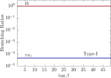
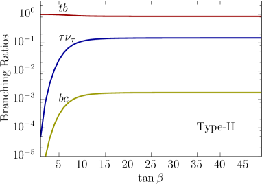
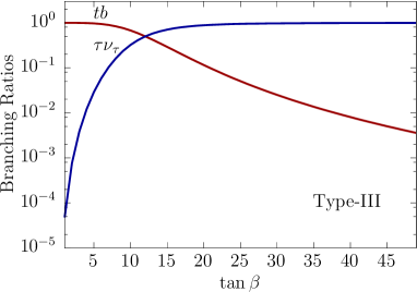
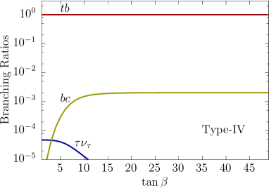
Figure 1: Charged Higgs branching ratios for four classes of 2HDM, setting $m_{H}=m_{A}=m_{{H}^{\pm}}=500$ GeV and $\sin(\beta-\alpha)=$1.

In Type I model, due to the $\cot\beta$ dependence of coupling, the $\text{Br}\left({{{H}^{+}}\rightarrow{\tau}^{+}\nu_{\tau}}\right)$ is suppressed by $m_{\tau}^{2}/m_{t}^{2}$ over $\text{Br}\left({{{H}^{+}}\rightarrow{t}\bar{b}}\right)$, leading almost 100% Br to $\bar{t}b$ mode. The dominant decay mode of charged Higgs in Type II model, as expected is in the $\bar{t}{b}$ channel, following sub-dominant $\bar{\tau}\nu_{\tau}$ channel with Br $\leavevmode\nobreak\ \sim 10-15$ %, followed by other suppressed modes such as, ${H}^{+}\to\bar{b}{c},{c}\bar{s}$. However, in the case of Type III model, which is lepton specific, the charged Higgs decays to $\bar{\tau}\nu_{\tau}$ mode dominantly, except in the lower region of $\tan\beta\sim 1-12$ where $t\bar{b}$ mode becomes important. On contrary, $\bar{\tau}\nu_{\tau}$ mode gets suppressed in Type IV model, because of $\cot\beta$ dependence, and $\bar{t}b$ channel takes over. It is to be noted that the pattern of these Brs expected to be different in the presence of ${H}^{\pm}\to{W}^{\pm}\phi,\ \ \left(\phi={h},{H},{A}\right)$ mode, of which decay width is proportional to $\cos\left(\beta-\alpha\right)$ leading it dominant ($\sim 100\%$) for the choice of $\sin(\beta-\alpha)=0$ . Interestingly, in the case of SUSY motivated Higgs sector, i.e in Type II model, if kinematically allowed, the charged Higgs can decay also to chargino and neutralino pair, ${H}^{\pm}\to\tilde{\chi}^{\pm}_{i}\tilde{\chi}_{j}^{0};$ (i:1-2, j:1-4), which may be dominant for Higgsino like scenario [58]. As pointed out earlier, that the charged Higgs sector is severely constrained by flavor physics data in addition to the direct searches of which details can be found in reviews [42, 27].

3 Charged Higgs production

In the intermediate to heavier mass range (${m_{{H}^{\pm}}}\gtrsim m_{t}$), the charged Higgs is produced directly in proton-proton collision via the process,

$${pp}\to{t}{H}^{-}+X.$$ (3.1)

At the parton level, the production mechanism is initiated via two subprocesses,

$${gg},{q}\bar{q} \leavevmode\nobreak\ \rightarrow\leavevmode\nobreak\ \leavevmode\nobreak\ {t}\bar{b}{H}^{-} \left(\text{4FS}\right)$$

$${gb} \rightarrow\leavevmode\nobreak\ \leavevmode\nobreak\ {t}{H}^{-} \left(\text{5FS}\right)$$ (3.2)

in 4 flavor(4FS) and 5 flavor scheme(5FS) at the leading order(LO) respectively. In fact, the process in 4FS is part of the NLO QCD correction to the 5FS scheme mechanism. The total NLO QCD effects to the inclusive ${H}^{\pm}$ production is essentially the NLO correction to the process ${gb}\to{tH}^{-}$ plus the total contribution due to the tree-level processes [59]. In 5FS, the NLO QCD corrections are known for sometime in the literature [60, 61, 62, 63], and also very recently approximate NNLO calculations also published [64]. The total theoretical uncertainty in ${H}^{\pm}$ production in association with top quark(5FS) is found to be of the range 15-20% [65]. In the 4FS, the final state bottom quark which originates due to the hard scattering is assumed to have non zero mass, where as in 5FS, the $b$ quark is treated as massless, and being part of the parton flux. In 4FS, the corresponding NLO correction estimated to be around 20% for the lower range of $m_{{H}^{\pm}}$, and it goes up little for more higher masses [65].

At finite order, the cross section in 4FS does not match with 5FS, as expected, due to different ways of treating perturbative calculation. However, it is expected that the results will match within the respective uncertainties once taking into account of all orders in perturbation. In order to obtain the precise estimation of charged Higgs production cross section, one needs to combine the 4 and 5 flavor scheme predictions appropriately. This combination is performed following the prescription, so called Santander-matching [66]. In the IR limit ($\frac{m_{{H}^{\pm}}}{m_{b}}\rightarrow 1$), the cross sections obtained from 4FS and 5FS scheme match nicely. The main difference between the 4FS and 5FS occurs because of the presence of large logarithm, which arises due to the splitting of incoming gluon into two nearly collinear b quarks [67]. Thus, the calculated cross sections using two schemes should be combined in such a manner that such logarithmic effects are taken into account appropriately. The prescription to match these cross sections computed in two schemes is given by [11, 65],

$$\sigma=\frac{\sigma^{\text{4FS}}+w\sigma^{\text{5FS}}}{1+w}\ \ {\rm with}\ \ w=\ln\frac{m_{{H}^{\pm}}}{m_{b}}-2.$$ (3.3)

Similarly, the theoretical uncertainties are combined as,

$$\Delta\sigma=\frac{\Delta\sigma^{\text{4FS}}+w\Delta\sigma^{\text{5FS}}}{1+w}\ \ {\rm with}\ \ w=\ln\frac{m_{{H}^{\pm}}}{m_{b}}-2.$$ (3.4)

With this matching methodology, the overall theoretical uncertainty of the combined NLO cross section is found to be around 10%, where as the individual 4FS and 5FS cross sections at NLO are in reasonable agreement within $\sim$ 20% from the central value [65, 11]. The production cross section and the corresponding uncertainty are very sensitive to $\tan\beta$, owing to the dependence of Yukawa coupling on it. The scale of uncertainty reduces with the decrease of $\tan\beta$ through the correction of bottom Yukawa coupling, which is proportional to $\tan\beta$. We first estimate the charged Higgs boson production in Type II 2HDM motivated by the SUSY providing inputs $\tan\beta$ and $m_{{H}^{\pm}}$, and then predict the corresponding cross sections for other classes of 2HDM(Type I, III and IV) simply by appropriately rescaling the couplings. It is to be noted that in the MSSM, the NLO QCD corrections may involve additional loop contributions from gluinos and squarks, which also depend on $\tan\beta$. This extra contribution can be absorbed through the rescaling of the the NLO QCD prediction of the bottom Yukawa coupling [68]. The total cross section primarily governed by the ${tb}{H}^{\pm}$ coupling is found to be minimum in strength for $\tan\beta\approx 7-8$.

Table 2: Charged Higgs boson production cross sections(in fb) in 4FS and 5FS schemes, at $\sqrt{s}=13$ TeV and $\tan\beta=30$ in Type II model and the last row presents cross sections for Type I. $\mu$ and $m_{b}(\mu)$ represent the QCD scales and mass of bottom quark at the scale $\mu$.

$m_{{H}^{\pm}}$ (GeV)$\to$	300	500	600	800	1000
$\mu$ (GeV)	236.5	336.5	386.5	486.5	586.5
$m_{b}\left(\mu\right)$ (GeV)	2.64	2.58	2.56	2.51	2.48
$\sigma\left({pp}\rightarrow{tbH}^{\pm}\right)$ (4FS) LO	290.2	60.4	30.6	9.0	3.1
$\sigma\left({pp}\rightarrow{tbH}^{\pm}\right)$ (4FS) NLO	359.4	73.3	39.9	11.4	4.1
$\sigma\left({pp}\rightarrow{tH}^{\pm}\right)$ (5FS) LO	581.3	126.0	64.8	19.7	6.9
$\sigma\left({pp}\rightarrow{tH}^{\pm}\right)$ (5FS) NLO	748.6	166.2	86.1	26.5	9.3
Matched (NLO)	625.3	140.9	74.1	22.8	8.1
Matched (NLO) (Type 1)	2.9	$0.66$	$0.35$	$0.11$	$3.9\times 10^{-2}$

In Table 2, the charged Higgs boson production cross sections for both schemes, and the final matched values are presented for few representative choices for $m_{{H}^{\pm}}$ and $\tan\beta=30$ in Type II model. The cross sections are computed both at LO and NLO, using MadGraph5-2.6.1 [69], with the FeynRules [70] model file uploaded by authors of [71]. We notice that for $\tan\beta=3$, the cross sections go down by a factor of $\sim\frac{1}{2}$ in Type II model. In calculating these cross sections, factorization and renormalization scales are set as, $\mu^{2}=\left(\frac{{m_{{H}^{\pm}}}+m_{t}}{2}\right)^{2}$, as shown in the first row along with the value of running b-quark mass[72]. Variation of cross sections are found to be within a range from ${\cal O}(100)$fb to ${\cal O}(1)$fb corresponding to the range $m_{{H}^{\pm}}$ $\sim$ 300 - 1000 GeV.

In Type I model (see Table 1), the charged Higgs boson couplings with top and bottom quark go by $\sim(m_{b}+m_{t})\cot\beta$. The cross sections in Type I model simply can be obtained from the values corresponding to Type II model by rescaling the Yukawa couplings [71, 65, 11]. The total cross section can be parameterized by $\sigma_{{H}^{\pm}}^{\text{Type II}}\propto{g}_{t}^{2}\sigma_{t}\cot^{2}\beta+g_{b}\sigma_{b}\tan^{2}\beta+g_{t}g_{b}\sigma_{tb}$, where, $g_{t}$ and $g_{b}$ are the part of the Yukawa couplings proportional to top and bottom quark masses respectively. Evaluating the contributions by setting $m_{t}=0({\text{i.e }}g_{t}=0)$ and $m_{b}=0({\text{i.e }}g_{b}=0)$, $\sigma_{b},\sigma_{t}$ and $\sigma_{bt}$ can be obtained. Thus, the cross sections in Type I model can be estimated rescaling each contribution by $\cot\beta$. This prescription works in to all orders in QCD, but not appropriate to all orders in the electroweak corrections [11].

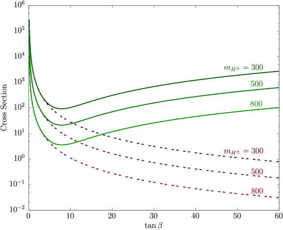
Figure 2: Matched charged Higgs production cross section(fb) at $\sqrt{s}=13$ TeV for three different masses(in GeV) in Type II (green/solid) and Type I (red/dashed) 2HDM.

The cross sections for both in Type I and II 2HDM are presented in Fig. 2 for various values of $\tan\beta$ and three choices of $m_{{H}^{\pm}}=300$ GeV, 500 GeV and 800 GeV. Clearly, as expected, the cross sections in Type I model are suppressed over Type II model by approximately $\sim\tan^{2}\beta$, for $\tan\beta\gg 1$. The cross sections in Type III(Type IV) model are the same as the Type I(Type II) due to the identical Yukawa coupling structures with quarks. A dip is observed for Type II model around $\tan\beta\sim 7-8$ unlike Type I, which can be understood from the respective couplings dependence on $\tan\beta$ or $\cot\beta$.

4 Signal and Background

As mentioned before, in this current study, the signature of charged Higgs boson is explored with its decay mode, ${{H}^{+}}\rightarrow{t}\bar{b}$. The $\text{Br}\left({{{H}^{+}}\rightarrow{t}\bar{b}}\right)$ is almost dominant, more than 70% for a wide range of $\tan\beta$, and for all classes of 2HDM as shown in Fig. 1, except for the Type III model which is lepton specific. Signal is simulated considering ${H}^{\pm}$ production mechanisms, Eq.3.2, and eventually the final results are obtained by combining them following the recipe, given in Eq.3.3.

The resulting signal final state consists multiple top quarks via the following processes:

$$\begin{array}[]{ccccccc}5\text{FS}&:&{gb}&\rightarrow&{tH}^{-}&\rightarrow&{t}\bar{t}{b}\\ 4\text{FS}&:&{gg}&\rightarrow&{t}\bar{b}H^{-}&\rightarrow&{t}\bar{b}\bar{t}{b}\end{array}$$ (4.1)

Both leptonic and hadronic final states are considered following the semi leptonic and hadronic decays of the top quarks respectively. Note that the final states consist multiple $b$ quarks, a characteristics of the heavier charged Higgs signal for the ${{H}^{+}}\rightarrow{t}\bar{b}$ decay channel [51, 52]. The top quark originating from ${H}^{\pm}$ decay is tagged in it’s hadronic mode, and combined with the appropriately identified $b$-jet, the charged Higgs mass reconstructed. Tagging of top quark is performed implementing the powerful jet substructure analysis[73], which is postponed for discussion in the next section. In case of pure hadronic signal final state, the associated top quark is also identified through kinematic reconstruction in order to make signal more robust. In addition to the reconstruction of top quarks, we exploit the presence of extra hard b-jets in the final state in order to separate out backgrounds. Therefore, we focus the charged Higgs signal final state in two categories:

$$\begin{array}[]{ccccccc}\text{a}&:&{H}_{\text{reco}}^{\pm}&+&{t}_{\text{reco}}&+&\text{n}_{b}\left(\geq 1\right)\leavevmode\nobreak\ {b}-\text{jet}\\ \text{b}&:&{H}_{\text{reco}}^{\pm}&+&\text{n}_{\ell}\left(\geq 1\right)&+&\text{n}_{b}\left(\geq 1\right)\leavevmode\nobreak\ {b}-\text{jet}\end{array}$$ (4.2)

where ${H}^{\pm}_{\text{reco}}$ and ${t}_{\text{reco}}$ represent the reconstructed Charged Higgs and top quark, and $n_{\ell}$ and $n_{b}$ are the number of leptons and $b$-jets respectively and required to be at least one. The main dominant source of irreducible SM backgrounds are due to $t\bar{t}$, and inclusive hard QCD jet production. However, in both cases, extra b-jets may arise via gluon splitting in the initial state radiation. The QCD jet production becomes dominant source of irreducible background, in particular corresponding to the hadronic signal final state, due to the non-negligible mis-tagging probability of hard jets as a top jet. Moreover, the process $t\bar{t}{g}$ which predominantly produces the final state $t\bar{t}{b}\bar{b}$ is also taken into account in our background estimation. Before discussing the signal and background simulation strategy, we discuss briefly the top tagging methodology used in our simulation.

4.1 Top Tagging

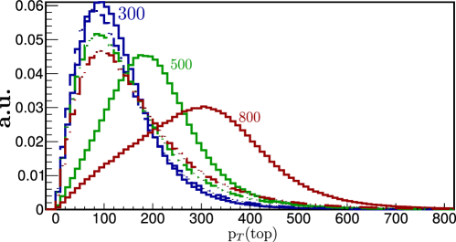
Figure 3: Parton level transverse momentum of top quark from charged Higgs decay(solid) and associated with it(dashed) for $m_{{H}^{\pm}}=300$ GeV, 500 GeV and 800 GeV, normalized to arbitrary units (a.u). The distribution of $p_{T}$ of top quark corresponds to the combined processes (Eq. 3.2) and then appropriately matched using Eq. 3.3.

The top tagged jets are the essential components of our considered signal events. It has been pointed out earlier that the top quark originating from ${H}^{\pm}$ decay is expected to be boosted(boost factor, $\gamma_{t}\sim m_{{H}^{\pm}}/m_{t}$), in particular for heavier charged Higgs boson masses. The $p_{T}$ of those top quarks are demonstrated in Fig. 3 for three masses of ${H}^{\pm}$, along with the same for associated top quarks. Clearly, this figure indicates that the top quark from heavier ${H}^{\pm}$ decay is moderately boosted, however, $p_{T}$ distribution of associated top quarks are found not so sensitive to $m_{{H}^{\pm}}$. A top quark decays to a $b$-quark and a $W$ which subsequently decays to a pair of light quarks leading to jets in the calorimeter. However, for fast top quark, these decay products may not appear well separated to resolve as a separate jets. In such cases, the boosted top quarks may look like a single jet, called fat jet with three or more subjets as constituent corresponding to its decay products. These subjets are well separated within an angular cone of the order $\sim 2m_{t}/p_{T}$. Following this kinematic features, we attempt to tag topjets, surrounded by busy hadronic environment using the top tagger, namely HepTopTagger [74, 75, 76, 77]. In the process of tagging tops, first cluster particles with $p_{T}\geq 0.5$ GeV and $|\eta|<5$, using the Cambridge/Aachen [78] jet algorithm implemented in Fastjet-3.3.0 [79] for jet radius R=1.5 to form fat jets. Then require at least one hard fat jet in the event with $p_{T}\geq 200$ GeV. In our searches, top tagged jets are likely to be contaminated by QCD radiation, since wider radius R=1.5 is considered to contain all subjets from the moderately boosted top quark decay. Therefore, it is suggestive to take extra measures to eliminate QCD effects due to soft radiation in reconstructing subjets. The sub structures of Fatjets are obtained following the mass drop method using some recursive steps which are built in HepTopTagger[74, 75, 76, 77]. In this process, the last step of clustering process is declustered to obtain two subjets $j_{1}$ and $j_{2}$, such that $m_{j_{1}}>m_{j_{2}}$. If $m_{j_{1}}+m_{j_{2}}\sim m_{j}$, and $m_{j_{1}}>0.8m_{j}$, then it is expected that $j_{2}$ originates from QCD emission or underlying events, and we discard $j_{2}$, otherwise we keep both $j_{1}$ and $j_{2}$. If the mass of the subjet is 30 GeV or less, then we keep it or decompose it further (both $j_{1}$ and $j_{2}$ or just $j_{1}$ depending on how symmetrically the mass splits). The subjets which are obtained at the end of the recursive declustering procedure, are also cleaned further through filtering [73] to eliminate the contamination from the QCD radiation. Two subjets are suppose to originate from $W$ decay, and it is ensured by requiring the invariant mass of two subjets $m_{jj}=m_{W}\pm 15$ GeV. Finally, the top is tagged by adding the third sub-jet, which is a $b$-like jet, examined by matching with the parton level b quark in the event. The invariant mass of three subjets after filtering is required to be $m_{jj{b}}=m_{t}\pm 30$ GeV. If there be more than one top tagged jet, we choose the one which is the closest to the pole mass of the top quark. Using the default conditions in HepTopTagger, we find the single top tagging efficiency is about 10% for this kind of moderately boosted tops in signal events. Note that in calculating this efficiency no pile-up effects are taken into account. The mistagging efficiencies are obtained using the QCD events and it is found to be around $2-3$ %.

We attempt to recover this top tagging efficiency to a better level by employing multivariate analysis. The multivariate analysis is implemented within TMVA [80] combining the HepTopTagger mass drop method, and instead of using the full chain of HepTopTagger, some other additional kinematic variables including N-Subjettiness, energy correlation, are used as listed below:

1. N-Subjettiness [81]: Variables are defined as,

   $$\frac{\tau_{2}}{\tau_{1}},\frac{\tau_{3}}{\tau_{2}},\frac{\tau_{4}}{\tau_{3}},$$ (4.3)

   where $\tau_{N}$ is the N-th subjettiness variable [82] as defined,

   $$\tau_{N}=\frac{1}{R_{0}\sum_{k}P_{T,k}}\sum_{k}P_{T,k}{\rm min}\left(\Delta R_{1,k},\Delta R_{2,k}...\Delta R_{N,k}\right)$$ (4.4)

   $\Delta R_{ik}$ is defined to be the geometrical separation between i-the subjet and the k-th reference axes, $R_{0}$ is the jet cone size parameter. Clearly, a smaller $\tau_{N}$ implies more radiation around the given axes, i.e a better description of jets with N or less subjets, where as large $\tau_{N}$ means a better description of jets with more than N subjets. It is found that $\tau_{N}/\tau_{N-1}$ is an efficient discriminating variable to distinguish boosted objects [82, 83, 81].

2. Mass difference: It is defined as, $\Delta m_{t}=|m_{j_{t}}-m_{t}|$, where $m_{j_{t}}$ is the mass of the tagged top jet. This mass difference is also very crucial in tagging tops.

3. Invariant mass of 2 and 3 subjets: Invariant mass of the 3 sub jets, $m_{123}$ and 2 sub jets $m_{ij}$ where $(i,j\in\left\{1,2,3\right\})$, is computed for each possible combination of subjets.

4. Number of $b$-like sub jets: The number of $b$-like sub jets $n_{b}^{j}$, it is counted by matching subjets with $b$-partons within $|\eta|<$ 2.5, and $p_{T}>5$ GeV using the matching cone $\Delta R<0.3$ around the subjet.

5. Variable related with reconstructed masses: It is defined to be,

   $$f_{\text{rec}}\equiv\min_{i,j}\left|\frac{\left(\frac{m_{ij}}{m_{123}}\right)}{\left(\frac{m_{W}}{m_{t}}\right)}-1\right|.$$ (4.5)

   This ratio determines the quality of reconstructed $W$ with respect to the overall quality of reconstructed top mass.

6. Energy correlations: The energy correlators among the subjets or particles inside a jet distinguishes the various properties of jets [84]. The correlation function uses the information about the energies and pair-wise angles between particles within a jet. This generalized energy correlation function, is interestingly can be made infrared and collinear safe. This energy correlation function is found to be very effective to classify jets. For details, see Ref.[84].

With these set of variables, 1-6, we train Boosted Decision Trees to tag top jets in $t\bar{t}$ and mis-tags in QCD process. In Fig.4, we show the results as a receiver operator response(ROC) curves for both signal acceptance and background(QCD) rejection efficiencies. This figure clearly demonstrates an improvement in top tagging efficiencies, along with the suppressed background mis-tag rates. The efficiencies obtained using HepTopTagger is also shown by a star. Undoubtedly, the top tagging efficiency through MVA method is improved significantly. We use this improved efficiency in the simulation of signal and background.

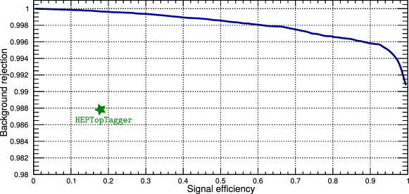
Figure 4: ROC curve for the MVA TopTagger obtained from signal events in hadronic final state and QCD for mis tagging. Efficiencies obtained using HepTopTagger is also shown.

4.2 Signal and Background Simulation

The PYTHIA8-8.2.26 (PYTHIA8) [85] is used to generate events via the process $gb\rightarrow t{H^{-}}$, where as MadGraph_aMC@NLO-2.6.1 (MG5) [69] is used for $gg\rightarrow t\bar{b}\text{H}^{-}$ and then showering through PYTHIA8. The dominant SM background processes $t\bar{t}$ and QCD events are generated using PYTHIA8, while MG5 interfacing with PYTHIA8 is used for $t\bar{t}{b}\bar{b}$ process. Events are generated by dividing the phase space in $\hat{p}_{T}$ bins, $\hat{p}_{T}$ is the transverse momentum of the final state partons in the center of mass frame. For instance, in case of signal events, bins are chosen as $0-200$ GeV, $200-400$ GeV and $400-\infty$, where as for backgrounds ($t\bar{t}$ and QCD), bins are set as $0-200$ ($20-200$ for QCD) GeV, $200-500$ GeV, $500-800$ GeV and $800-\infty$. Various event selections imposed in the simulation for both signal and backgrounds are described below:

1. Lepton selection: Leptons, both electrons and muons are selected with cuts on the transverse momentum($p_{T}^{\ell}$), and rapidity($\eta_{\ell}$),

   $$p_{T}^{\ell}\geq 20\leavevmode\nobreak\ {\rm GeV},\leavevmode\nobreak\ \leavevmode\nobreak\ \leavevmode\nobreak\ \leavevmode\nobreak\ \leavevmode\nobreak\ \left|\eta_{\ell}\right|\leq 2.5$$ (4.6)

   Isolation of lepton is ensured by requiring, $E_{T}^{AC}\leq$ 30% of $p_{T}^{\ell}$, where $E_{T}^{AC}$ is the sum of transverse momenta of the particles which are within the cone $\Delta R$(= $\sqrt{\Delta\eta^{2}+\Delta\phi^{2}}$) $<0.3$ along the direction of lepton. It is to be noted that the lepton isolation criteria is not imposed while selecting events applying lepton veto, otherwise genuine leptonic events would contribute to the hadronic events.

2. $b$-jet identification: In the simulation jets are reconstructed using Fastjet [79] with anti-$k_{T}$ algorithm [86] and jet size parameter R=0.5. Reconstructed jets are subject to $p_{T}^{j}>20$GeV, $|\eta_{j}|<4$. A given reconstructed jet identified as $b$-like jet, if there is a matching with parton level $b$ quark with a matching cone $\Delta R<0.3$. In addition, the matched jets are required to have $|\eta|<2.5$. We found about 70% cases $b$ quarks are identified as $b$-like jets Finally, in the simulation to select b-like jets, we apply a hard cut $p_{T}>$30 GeV. It is to be noted that in our simulation the mistags are not taken into account, which is out of the scope of the present analysis. However,from the studies [87, 88], we found that the mistags of the order of few percent are not expected to affect our results significantly.

3. Top reconstruction: The details of the top tagging are already discussed in the previous section. However among the tops tagged using this technique, we found 60-70% are from the decay of ${H}^{\pm}$ while the remaining are the associated tops, for the case of $m_{{H}^{\pm}}=500$ GeV and it goes up with the increase of $m_{{H}^{\pm}}$. In addition, after the reconstruction of charged Higgs using tagged top jets, an additional top quark is also reconstructed through kinematic fitting out of the remaining jets for hadronic signal events. This extra kinematically reconstructed top quark is likely to correspond to the associated top quark. For leptonic signal events no such top quark is reconstructed.

4. Charged Higgs mass reconstruction: We observed via matching that the leading identified $b$-jet with $p_{T}>50$ GeV corresponds ($\sim$ 70-80%) to $b$ quark originating from ${H}^{\pm}$ decay (for ${m_{{H}^{\pm}}}{\gtrsim}500$ GeV). Hence, the charged Higgs mass is reconstructed combining the leading top tagged jet with the leading $b$-like jet. In Fig.5, we show the reconstructed mass($m_{{t}_{j}{b}_{1}}$) of charged Higgs for three input values, $m_{{H}^{\pm}}=300$ GeV, 500 GeV, 800 GeV along with the dominant background from $t\bar{t}$ corresponding to hadronic final states, Eq. 4.2(a) subject to selection cuts on $b$-jets. The distribution due to $t\bar{t}b\bar{b}$ appears to be almost same as $t\bar{t}$, where as for QCD it comes out as flat without any visible peak. The distributions from both these sources are not shown in this Fig. 5, otherwise it would be very crowded. Notice that the peaks are not appearing exactly at the input mass of charged Higgs because of the smearing of the momenta of tagged top and $b$ jet. The wide spread of $m_{{t}_{j}{b}_{1}}$ distribution around the peak is due to incorrect combination of the reconstructed top and $b$-like jet. The events are selected requiring the reconstructed mass $m_{{t}_{j}{b}_{1}}$ within the range,

   $$m_{{t}_{j}{b}_{1}}=m_{{H}^{\pm}}\pm 0.3\leavevmode\nobreak\ m_{{H}^{\pm}},$$ (4.7)

   which is 30% around the peak.

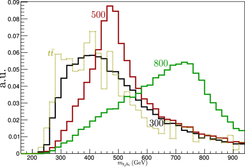
   Figure 5: Charged Higgs mass($=m_{{{t}_{j}}{b}_{1}}$, matched with 4FS and 5FS) reconstruction for $m_{{H}^{\pm}}=300$ GeV, 500 GeV and 800 GeV and $\tan\beta=30$ along with the background from $t\bar{t}$(dashed).

   

5. Multiplicity of $b$ jets: In signal events multiplicity of $b$-jets is higher than the $t\bar{t}$ and QCD backgrounds. Hard $b$-jet remains in signal final state, even after reconstruction of two(one) tops, and subsequently a charged Higgs in hadronic(leptonic) final state. The additional $b$-jets appearing in background events are due to the gluon splitting, and is not expected to be hard. Therefore, requirement of at least one hard $b$ jet in the final state is expected to be useful in rejecting backgrounds. Hence, a selection,

   $$n_{b}\geq 1\ \ {\rm with}\ \ p_{T}^{b}\geq 30\leavevmode\nobreak\ {\rm GeV}$$ (4.8)

   is imposed in the simulation.

4.3 Results

We simulate both the production processes in 4FS and 5FS, and then obtain the final yield by appropriately weighting both the resulting cross sections, as per prescription given by Eq. 3.3 and 3.4. For the illustration purpose, in Table 3, the event yields in terms of cross sections are presented after each set of cuts as described above, for signal and backgrounds corresponding to the hadronic final state, see Eq. 4.2(a). The second row shows the total production cross sections of the respective processes at 13 TeV center of mass energy. Results for signal events are shown only for a representative choice of a single mass of charged Higgs, $m_{{H}^{\pm}}=500$ GeV, although simulations are performed for a wide range of masses, upto 1 TeV. Also note that the results are presented for $\tan\beta=30$ and within the framework of Supersymmetric based model (Type II). Fat jets are reconstructed selecting events with a lepton veto and at least one $b$-identified jets. In order to access the boosted region, events are selected with a $p_{T}>200$ GeV on fat jets. These high $p_{T}$ fat jets are used as a input to HepTopTagger to tag them as top jets. We employ MVA method as described above to tag top jets, and found that about 30% of events are tagged as a top jet. Subsequently, after top tagging, we look for the hardest leading $b$-jet with a cut $p_{T}>50$ GeV, which is found to be originating from ${H}^{\pm}$ decay for about 70-80% events. Combining top tagged jets and the hardest $b$ jet, the charged Higgs mass is reconstructed, and select events within the mass window $\pm 30\%$ of the input charged Higgs mass. Notice that a good fraction of background events remain within this reconstructed charged Higgs mass window. With the remaining untagged jets and identified $b$-jets, the associated top quark is reconstructed. The requirement of a second reconstructed top quark, suppresses the background, in particular QCD, more than the signal. Finally, demanding a hard $b$-jet with $p_{T}>30$ GeV rejects backgrounds substantially.

Table 3: Cross section yields for signal and backgrounds in the hadronic signal final state (Eq 4.2(a)) for ${m_{{H}^{\pm}}}=500$ GeV, $\tan\beta=30$ in Type II 2HDM. The first row presents the production cross sections. For signal, $\text{Br}\left({{{H}^{+}}\rightarrow{t}\bar{b}}\right)$ is multiplied with the signal cross sections.

Selection	5FS$\times$Br	4FS$\times$Br	$t\bar{t}$	$t\bar{t}{b}\bar{b}$	QCD
$\sigma$(fb)	$124.9$	$64.4$	$8.3\times 10^{5}$	$1.4\times 10^{4}$	$7.2\times 10^{11}$
$N_{b}\geq 1$ & Lepton Veto	$55.8$	$28.8$	$4.6\times 10^{5}$	$7.4\times 10^{3}$	$1.2\times 10^{10}$
$N_{\text{FJ}}\geq 1$	$44.8$	$24.2$	$1.1\times 10^{5}$	$2.6\times 10^{3}$	$9.4\times 10^{6}$
$N_{{t}_{j}}\geq 1$	$13.3$	$7.4$	$3.2\times 10^{4}$	$790.4$	$2.5\times 10^{5}$
$p_{T}^{{b}_{1}}\geq 50$ GeV	$12.3$	$6.9$	$2.0\times 10^{4}$	$633.5$	$9.2\times 10^{4}$
$m_{{t}_{j}{b}_{1}}\in\left[0.7m_{{H}^{\pm}},1.3m_{{H}^{\pm}}\right]$	$8.8$	$5.2$	$1.3\times 10^{4}$	$387.6$	$4.2\times 10^{4}$
$N_{{t}_{\text{Associated}}^{\text{Hadronic}}}=1$	$2.2$	$1.6$	$364.1$	$78.8$	$1.2\times 10^{3}$
Extra b, $p_{T}\geq 30$ GeV	$0.5$	$0.5$	$20.3$	$15.9$	$50.2$

Similarly cross section yields for leptonic final states(Eq.4.2(b)) are presented in Table 4. The events are selected with at least one identified $b$-jet and one isolated lepton. A top jet is tagged, and it is observed that efficiency of top tagging is less, due to the lack of availability of many hadronic top quarks. As before, requiring a hard identified $b$-jet, with $p_{T}>50$ GeV and combining it with tagged top jet, the charged Higgs mass is reconstructed. Finally, requirement of a hard $b$-jet suppresses the background more than the signal. Use of an additional cut on missing transverse momentum due to the presence of neutrinos in the leptonic decay of top quark is found to be not so helpful.

Table 4: Same as in Table 3, but for the leptonic signal final state.

Selection	5FS$\times\text{Br}$	4FS$\times\text{Br}$	$t\bar{t}$	$t\bar{t}{b}\bar{b}$	QCD
$\sigma$(fb)	$124.9$	$64.4$	$8.3\times 10^{5}$	$1.4\times 10^{4}$	$7.2\times 10^{11}$
$N_{b}\geq 1$ & $N_{\ell}\geq 1$	$39.3$	$20.3$	$2.5\times 10^{5}$	$4.2\times 10^{3}$	$5.0\times 10^{6}$
$N_{\text{FJ}}\geq 1$	$29.3$	$15.8$	$5.0\times 10^{4}$	$1.3\times 10^{3}$	$3.6\times 10^{3}$
$N_{{t}_{j}}\geq 1$	$5.4$	$3.0$	$1.0\times 10^{4}$	$276.1$	$103.1$
$p_{T}^{{b}_{1}}\geq 50$ GeV	$4.9$	$2.8$	$6.7\times 10^{3}$	$221.8$	$71.7$
$m_{{t}_{j}{b}_{1}}\in\left[0.7m_{{H}^{\pm}},1.3m_{{H}^{\pm}}\right]$	$3.4$	$2.0$	$4.4\times 10^{3}$	$138.3$	$20.5$
$p_{T}^{{b}_{2}}\geq 30$ GeV	$2.1$	$1.3$	$301.0$	$66.1$	$\lesssim 1.0$

Table 5: Cross sections (fb) normalized by acceptance efficiencies ($\epsilon_{\text{ac}}$) for signal and background. Signal significances for three integrated luminosity options for hadronic (leptonic) final state are performed for the Type II model and $\tan\beta=30$.

		$\sigma\times\epsilon_{\text{ac}}$ (in fb)
${m_{{H}^{\pm}}}{\rightarrow}$	300 GeV	500 GeV	800 GeV
5FS	0.4 $\left(1.4\right)$	0.5 $\left(2.1\right)$	0.1 $\left(0.51\right)$
4FS	0.3 $\left(0.95\right)$	0.5 $\left(1.3\right)$	0.1 $\left(0.34\right)$
$t\bar{t}$	5.9 $\left(140.0\right)$	20.3 $\left(301.0\right)$	15.5 $\left(142.3\right)$
$t\bar{t}{b}\bar{b}$	5.4 $\left(22.0\right)$	15.9 $\left(66.1\right)$	8.8 $\left(37.6\right)$
QCD	$\lesssim 1.0$ $\left(\lesssim 1.0\right)$	50.2 $\left(\lesssim 1.0\right)$	21.4 $\left(\lesssim 1.0\right)$
Matched Signal cross section(S)	0.4 $\left(1.3\right)$	0.5 $\left(1.9\right)$	0.1 $\left(0.47\right)$
Total Background cross section(B)	11.3 $\left(161.9\right)$	86.4 $\left(367.1\right)$	45.7 $\left(179.9\right)$
${\cal L}$ (fb-1)		$S/\sqrt{B}$
300	1.9 $\left(1.73\right)$	0.92 $\left(1.71\right)$	0.28 $\left(0.61\right)$
1000	3.4 $\left(3.16\right)$	1.7 $\left(3.13\right)$	0.51 $\left(1.11\right)$
3000	5.9 $\left(5.48\right)$	2.9 $\left(5.42\right)$	0.88 $\left(1.92\right)$

In Table 5, we summarize the signal and background cross sections normalized by the kinematic acceptance efficiencies for both the hadronic and leptonic final state respectively. For illustration, we show results for three choices of charged Higgs mass, $m_{{H}^{\pm}}=300$, 500 and 800 GeV, corresponding to the signal cross sections in both 4FS and 5FS mechanisms. The signal cross sections are found to be ${\cal O}$(fb), where as the total background contribution is huge, in particular for hadronic final state. But for leptonic final state, the level of background contamination is comparatively less. In this case, the presence of leptons and a hard $b$ jet requirement in the final state help to get rid of a good fraction of the QCD background.

The signal significances are presented for three integrated luminosity options ${\cal L}=300$, 1000 and 3000 $\text{fb}^{-1}$. Table 5 reveals that the charged Higgs boson of mass 300 GeV can be discovered for high luminosity options(3000 $\text{fb}^{-1}$) with a reasonable significance, but for higher masses $\sim 500$ GeV or more, the signal is merely observable. Clearly, it is hard to achieve discoverable signal sensitivity for heavier charged Higgs mass in this channel. However, discovery potential of charged Higgs in leptonic final state is comparatively better. For instance, Table 5 shows that the charged Higgs signal observable with a moderate significance for the mass range around 500 GeV even for 1000 $\text{fb}^{-1}$ integrated luminosity option.

In summary, undoubtedly, this cut based analysis indicates how difficult it is to achieve discoverable sensitivity of charged Higgs signal in the ${t}\bar{b}$ decay mode owing to the huge background cross section with identical event topology. The present set of cuts are not very efficient to suppress backgrounds at the required level in order to make signal sensitivity better. One may think of more better construction of kinematic observables, and devise a set of cuts providing efficient optimization to reduce the background effect. It is a very challenging task to find the feasibility of the charged Higgs signal for heavier masses at the LHC. It motivates us further to develop a search strategy using the technique of multivariate analysis, which is discussed in the next section.

5 Multivariate Analysis

In the previous section, we observed that there is no single or a combination of kinematic variables which has the potential to isolate tiny signal out of huge backgrounds. In this section, we discuss MVA in order to improve signal to background ratio aiming to achieve a better significance for a given luminosity option. The basic idea of this method is to combine many kinematic variables which are the characteristics of signal events, into a single discriminator, and eventually this single discriminator is used to separate out the signal suppressing backgrounds. The MVA framework is a powerful tool used very widely in high energy physics, to extract the tiny signal events out of huge background events, including single top discovery [89] and recently the Higgs boson at the LHC [90]. Here we carry out MVA through Boosted Decision Tree(BDT) method within the framework of TMVA [80].

In the BDT method, events are classified by applying sequentially a set of cuts making sub sets of events with different signal purity. Several disjoint decision trees consisting two branches are constructed through a best selection of cuts out of listed input variables of the given process, and it is repeated using subsequent set of cuts till all the events are classified. While training the sample events, if an event is misclassified i.e a signal event labeled as background or background event as signal event, then it is boosted by increasing the weight of that event. Subsequently, a second tree is made using the new weights, which may not be same as the previous tree. This process is repeated and we constructed about 1000 trees. There are few methods of boosting [91], and we use the gradient boosting technique [92]. In BDT algorithm, these trees are made by training half of the signal and background events. The remaining half of the signal and background events are used to check the performance of the trained BDT.

Following the production and decay mechanism, Eq. 4.1, events are selected for the final state consisting one top tagged jet, more than one identified $b$ jet and untagged jets corresponding to hadronic signal final state. For leptonic signal, in addition, at least one isolated lepton is required. A large number of kinematic variables are constructed out of the momenta of these objects to train event samples, and eventually 10 input variables are used in BDT to train signal and background sample. In Table 6 and 7, the set of input variables are shown ranking them according to the importance in the BDT analysis for ${m_{{H}^{\pm}}}=500$ GeV corresponding to hadronic and leptonic final states respectively. In the third row of this table a brief description is provided for each of the variables. The importance here means the effectiveness of those variables in suppressing backgrounds while maintaining a better signal purity.

Table 6: Kinematic variables used to train the signal and background sample for hadronic final state and $m_{{H}^{\pm}}=500$ GeV.

Rank	Variables	Description
1	$m_{{b}\bar{b}}^{12}$	Invariant mass of two b jets
2	$p_{T}^{j}$	$p_{T}$ of the leading jet
3	TaggedTopMVA	MVA Discriminator for Toptagging
4	$m_{{b}_{1}{b}_{2}{b}_{3}}$	Invariant mass of 3 bjets
5	$p_{T_{2}}^{{b}_{\text{jet}}}$	$p_{T}$ of 2nd b jet after top tagging
6	$m^{\text{reco}}_{{t}_{j}{b}_{1}}$	Reconstructed Higgs mass
7	$H_{T}$	Scalar sum of $p_{T}$ of all final detectable particles
8	$n_{j}$	Number of un tagged
9	$p_{T_{3}}^{{b}_{\text{jet}}}$	$p_{T}$ of 3rd b jet
10	$H_{T}^{b}$	Scalar sum of $p_{T}$ of all b jets

Table 7: Same as Table 6, but for leptonic final state.

Rank	Variables	Description
1	$H_{T}^{b}$	Scalar sum of $p_{T}$ of all b jets
2	$m_{{t}_{j}}$	Mass of the tagged top jet
3	$m_{{b}\bar{b}}^{12}$	Invariant mass of two b jets
4	$m_{{t}{{b}_{2}}}$	Invariant mass of tagged top jet and second b jet
5	$H_{T}/{\text{MHT}}$	Ratio over $H_{T}$ and MHT
6	$p_{T}^{j_{1}}$	$p_{T}$ of leading un tagged jet
7	$H_{T}$	Scalar sum of $p_{T}$ of all jets
8	$p_{T}^{{b}_{\text{jet}}}$	$p_{T}$ of leading b jet
9	$p_{T_{2}}^{{b}_{\text{jet}}}$	$p_{T}$ of $2^{\text{nd}}$ b jet after top tagging
10	MHT	Vector sum of $p_{T}$ of all jets and leptons

We have observed that for ${m_{{H}^{\pm}}}=300$ GeV, the importance or ranking of some of the variables are altered. For example, for 300 GeV, $p_{T_{3}}^{{b}_{\text{jet}}}$ and $H_{T}^{b}$ are found to be more important than $m^{\text{reco}}_{tb}$. Similarly, for very heavier charged Higgs mass, the $H_{T}$ is expected to be more important in suppressing background, hence it is ranked to second. Interestingly, the invariant mass of the first two leading $b$ jets seems to be a very strong discriminant variable in separating the signal and background. Moreover, the MVA discriminator for top tagging using HepTopTagger, multiplicity of untagged jets, and $p_{T}$ of the second $b$-jet, all appear to be useful variables in eliminating the background events.

In Table 7, the set of kinematic variables are presented for leptonic final state and for ${m_{{H}^{\pm}}}=500$ GeV. However, as before, this set remains same for ${m_{{H}^{\pm}}}=300$ and 1000 GeV, but ranking becomes different for obvious reasons. For instance, for lower mass of ${m_{{H}^{\pm}}}=500$ GeV, the variable 3 becomes more important than the variable 1. Due to the presence of neutrinos, the variable related with missing transverse energy, MHT plays role in discriminating background, in particular from QCD. Like hadronic case, the number of $b$ jets and their corresponding transverse momentum are very effective in increasing signal to background ratio.

In this type of analysis based on machine learning models, one of the issue often encountered is the problem of overtraining the sample. The training of the sample can be checked using a test data sample. Ideally, for a sufficiently large and random monte carlo data, performance of training and testing data should be similar. If a significant deviations between these two are found, that would be an indication of over training of the sample. This overtraining tests are performed for all ${m_{{H}^{\pm}}}=300-1000$ GeV masses.

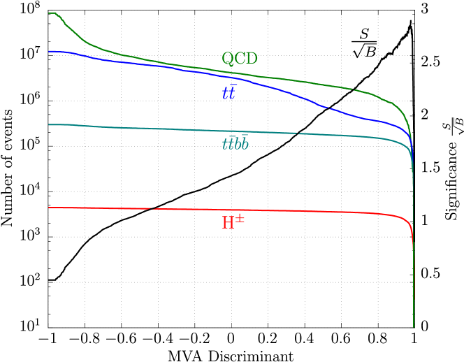
Figure 6: MVA output (D) distribution for signal and backgrounds corresponding to hadronic signal final state and ${m_{{H}^{\pm}}}=500$ GeV, $\tan\beta=30$ for Type II 2HDM.

In Fig. 6, the distribution of MVA output discriminator (D) with the number of events are presented, for signal events with ${m_{{H}^{\pm}}}=500$ GeV and backgrounds from QCD, $t\bar{t}$ and $t\bar{t}b\bar{b}$, along with the significance $S/\sqrt{B}$ for an integrated luminosity 300 $\text{fb}^{-1}$. Significance close to $3\sigma$ can be achieved with a selection of the discriminator, $\text{D}>0.9$. With this cut on D, and for integrated luminosity of 300 fb^-1, the number of events turn out to be 2830 for signal, and 1140000 for total backgrounds, where 70% contribution come from QCD. The selection of $D>0.9$ leads to a significance $\sim 2.65\sigma$ which goes up more for higher luminosity options.

Unlike the hadronic case, in the leptonic signal final state (see Fig. 7), the dominant background appears to be due to $t\bar{t}$ production. A cut on BDT output $\text{D}>0.9$ leads to a significance of about 3$\sigma$ for ${\cal L}=300\text{ fb}^{-1}$. The study is extended upto the 1000 GeV mass of the charged Higgs.

Signal significances are presented for both hadronic and leptonic final state(in parenthesis) in Table.8 for three masses of charged Higgs and for three integrated luminosity options. Remarkably, using MVA technique a significant improvement in sensitivity for both hadronic and leptonic signal is achieved. This table suggests that in hadronic channel the charged Higgs boson of mass upto $\sim$ 500 GeV can be probed with a reasonable sensitivity, much better than the obtained using simple cut based analysis as shown in, Table 5.

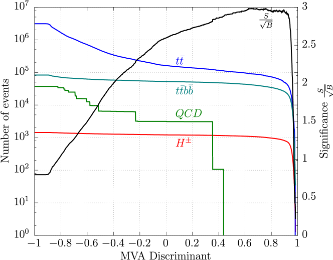
Figure 7: Same as for Fig. 6, but for leptonic signal.

Table 8: Significances for hadronic (leptonic) final states and for three luminosity options, in SUSY motivated Type II model with $\tan\beta=30$.

		$S/\sqrt{B}$
${m_{{H}^{\pm}}}(GeV){\rightarrow}$	300	500	800	1000
${\cal L}=300$ fb-1	$6.1$ $\left(5.2\right)$	$2.7$ $\left(2.94\right)$	$0.61$ $\left(0.96\right)$	$0.22$ $\left(0.39\right)$
${\cal L}=1000$ fb-1	$11.0$ $\left(9.5\right)$	$4.8$ $\left(5.4\right)$	1.1 $\left(1.7\right)$	$0.40$ $\left(0.71\right)$
${\cal L}=3000$ fb-1	$19.1$ $\left(16.5\right)$	$8.4$ $\left(9.3\right)$	1.9 $\left(3.0\right)$	$0.70$ $\left(1.2\right)$

The Table 8 shows that the signature of charged Higgs of mass around 800 GeV is observable in leptonic channel for 3000 $\text{fb}^{-1}$ luminosity option unlike the hadronic final state. For lower range of masses($\sim$ 500 GeV) signal is feasible even for 1000 $\text{fb}^{-1}$ luminosity option.

The results presented in Table 8 correspond to the SUSY motivated Type II model. However, the signal cross sections for other classes of 2HDM can be obtained out of these estimated values simply by rescaling the couplings and appropriately multiplying $\text{Br}\left({{{H}^{+}}\rightarrow{t}\bar{b}}\right)$. The significances for all four types of models are presented for both both hadronic and leptonic(within the parenthesis) in Table 9 and  10, corresponding to $\tan\beta=30$ and 3 respectively. Table 9 suggests that for high $\tan\beta$ scenario, discovery potential of charged Higgs in the context of Type II and Type IV model is quite promising for masses upto around 600-700 GeV, however, due to little increase($\sim$ 20%) of Br$\left({{H}^{+}}\rightarrow{t}\bar{b}\right)$, sensitivity is better for Type IV model. Because of the suppressed coupling of charged Higgs with top and bottom quarks, for high $\tan\beta$ scenario, the signal sensitivity is very poor for both Type I and III model. However, for low $\tan\beta$ scenario(10), results suggest that discovery potential is quite promising for this kine of model parameter space. Interestingly significances corresponding to all types of model, are found to be almost same for a given mass and luminosity option. It can be attributed to the fact, that in all classes of 2HDM, the dominant part of charged Higgs couplings proportional to $m_{t}\cot\beta$ which results the same significances.

Table 9: Sensitivity($S/{\sqrt{\rm B}}$) for hadronic (leptonic) signal events corresponding to all 4 types of 2HDM, and $\tan\beta=30$, $\sin\left(\beta-\alpha\right)=1$.

$m_{{H}^{\pm}}$ (GeV)	${\cal L}$ (in fb-1)	Type I	Type II	Type III	Type IV
	300	0.043 $\left({0.037}\right)$	$7.4$ $\left({6.4}\right)$	$0.0007$ $\left({0.0006}\right)$	$9.270$ $\left({7.999}\right)$
300	1000	$0.08$ $\left({0.07}\right)$	$13.5$ $\left({11.6}\right)$	$0.001$ $\left({0.001}\right)$	$16.925$ $\left({14.603}\right)$
	3000	$0.14$ $\left({0.12}\right)$	$23.3$ $\left({20.1}\right)$	$0.002$ $\left({0.002}\right)$	$29.316$ $\left({25.294}\right)$
	300	$0.017$ $\left({0.019}\right)$	$3.1$ $\left({3.4}\right)$	$0.0004$ $\left({0.0004}\right)$	$3.621$ $\left({4.017}\right)$
500	1000	$0.031$ $\left({0.034}\right)$	$5.6$ $\left({6.2}\right)$	$0.0007$ $\left({0.0009}\right)$	$6.611$ $\left({7.335}\right)$
	3000	$0.053$ $\left({0.059}\right)$	$9.8$ $\left({10.8}\right)$	$0.001$ $\left({0.001}\right)$	$11.451$ $\left({12.704}\right)$
	300	$0.004$ $\left({0.006}\right)$	$0.71$ $\left({1.1}\right)$	$0.0001$ $\left({0.0002}\right)$	$0.823$ $\left({1.294}\right)$
800	1000	$0.007$ $\left({0.011}\right)$	$1.3$ $\left({2.0}\right)$	$0.0002$ $\left({0.0003}\right)$	$1.502$ $\left({2.363}\right)$
	3000	$0.01$ $\left({0.02}\right)$	$2.2$ $\left({3.5}\right)$	$0.0003$ $\left({0.0005}\right)$	$2.601$ $\left({4.093}\right)$

Table 10: Same as Table.9, but with $\tan\beta=3$.

$m_{{H}^{\pm}}$ (GeV)	${\cal L}$ (in fb-1)	Type I	Type II	Type III	Type IV
	300	$4.3$ $\left({3.7}\right)$	$4.3$ $\left({3.7}\right)$	$4.3$ $\left({3.7}\right)$	$4.3$ $\left({3.7}\right)$
300	1000	$7.8$ $\left({6.7}\right)$	$7.9$ $\left({6.8}\right)$	$7.9$ $\left({6.8}\right)$	$7.8$ $\left({6.7}\right)$
	3000	$13.5$ $\left({11.7}\right)$	$13.7$ $\left({11.8}\right)$	$13.7$ $\left({11.8}\right)$	$13.5$ $\left({11.7}\right)$
	300	$1.7$ $\left({1.9}\right)$	$1.7$ $\left({1.9}\right)$	$1.7$ $\left({1.9}\right)$	$1.7$ $\left({1.9}\right)$
500	1000	$3.1$ $\left({3.4}\right)$	$3.1$ $\left({3.5}\right)$	$3.1$ $\left({3.5}\right)$	$3.1$ $\left({3.4}\right)$
	3000	$5.3$ $\left({5.9}\right)$	$5.4$ $\left({6.0}\right)$	$5.4$ $\left({6.0}\right)$	$5.3$ $\left({5.9}\right)$
	300	$0.39$ $\left({0.62}\right)$	$0.40$ $\left({0.63}\right)$	$0.40$ $\left({0.63}\right)$	$0.39$ $\left({0.62}\right)$
800	1000	$0.72$ $\left({1.1}\right)$	$0.73$ $\left({1.1}\right)$	$0.73$ $\left({1.1}\right)$	$0.72$ $\left({1.1}\right)$
	3000	$1.2$ $\left({2.0}\right)$	$1.3$ $\left({2.0}\right)$	$1.3$ $\left({2.0}\right)$	$1.2$ $\left({2.0}\right)$

The discovery potential of charged Higgs of mass 300 GeV, in the $\bar{t}{b}$ decay channel is quite promising even for 300 $\text{fb}^{-1}$ luminosity option at 13 TeV energy. However, for higher masses, e.g. for $m_{{H}^{\pm}}=500$ GeV, one needs high luminosity options such as 1000 $\text{fb}^{-1}$ and more. This study shows that for higher masses $\sim$ 1000 GeV, it is very hard to achieve better signal sensitivity even for high luminosity option.

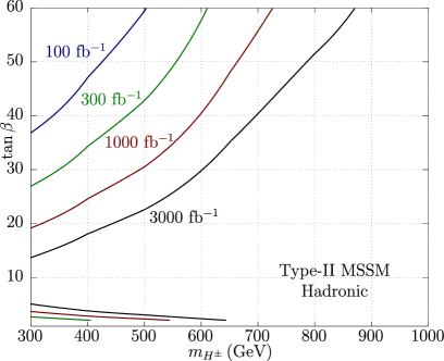
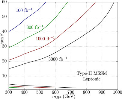
Figure 8: Discovery region for a given luminosity(in $\text{fb}^{-1}$) options in the context of SUSY(Type II) model for hadronic(left) and leptonic(right) final state at $\sqrt{s}=13$ TeV.

Finally, in Fig. 8 the discovery region is presented in the $m_{{H}^{\pm}}-\tan\beta$ plane in the context of SUSY motivated Type II model, requiring a 5$\sigma$ significance for a given luminosity options, as shown in the figure. Contours show that the minimum value of $\tan\beta$ required to discover charged Higgs of given mass mass at $5\sigma$ level for a given luminosity option. The parameter space above the contours are discoverable corresponding to that luminosity option at $\sqrt{s}=$13 TeV energy. In hadronic channel, even for high luminosity option, it is very hard to find charged Higgs of mass beyond 850 GeV. On the other hand, for the leptonic final state, charged Higgs can be explored almost upto $m_{{H}^{\pm}}\sim$1 TeV with high luminosity. Discovery regions below the contours for much lower $\tan\beta$ are also shown with three luminosity options. For a given $m_{{H}^{\pm}}$, the lowest $\tan\beta$ corresponds to 3000$\text{fb}^{-1}$ and then decreases to 1000$\text{fb}^{-1}$ and 300$\text{fb}^{-1}$ for other two lines respectively.

It is to be noted that while calculating the signal significance, the uncertainties of the background are not taken into account. The estimation of systematics in the background evaluation is currently out of the scope for the present analysis. However, due to the tiny signal size in comparison to background events, i.e with less purity, the impact of systematic uncertainties is expected to be severe. It can be understood by evaluating the significance as, S/${\sqrt{B+(\delta B)^{2}}}$, where $\delta$ stands for the level of uncertainties. For instance, corresponding to moderate range of charged Higgs masses, and for about 20% uncertainties in background estimation, the signficances go down drastically, for both hadronic and leptonic case. For heavier mass range, $m_{{H}^{\pm}}\sim$ 800 GeV, the impact of systematics to significance is not that severe due to less number of background events. Clearly, in order to achieve a reasonable significance to discover the charged Higgs for the intermediate mass range, one needs to perform the background estimation as precisely as possible.

6 Summary

In this study, we explore the detection prospect of the charged Higgs boson for the heavier mass range at the LHC in Run 2 experiments with the center of mass energy, $\sqrt{s}=13$ TeV, within the framework of generic 2HDM. A very brief discussion of 2HDM is presented in order to set up model framework to carry out the analysis. It is observed, that in all classes of 2HDM, the $\text{Br}\left({{{H}^{+}}\rightarrow{t}\bar{b}}\right)$ always the dominant one, except in Type III model where it holds only for lower range of $\tan\beta\left(<10\right)$. It is to be noted that the other decay modes, such as ${H}^{\pm}\to{W}^{\pm}\phi$ $\left(\phi\in\left\{h,H,A\right\}\right)$ also open up with a large Br once the condition $\sin(\beta-\alpha)=1$ is relaxed, as discussed in Sec.2. The charged Higgs boson production cross section at $\sqrt{s}=13$ TeV are computed in both 4FS and 5FS mechanisms, and finally the matched values are presented for a few representative choices of $m_{{H}^{\pm}}$. In the context of SUSY motivated Type II model, the matched cross sections vary from ${\cal O}$(100 fb) to ${\cal O}$(10 fb) for the range of $m_{{H}^{\pm}}\sim 300-1000$ GeV corresponding to large values of $\tan\beta$, and found to be less for other classes of 2HDM. The signature of charged Higgs is analyzed for the final state consisting of a reconstructed charged Higgs mass and extra $b$-jets plus an additional reconstructed top quark for hadronic events, while in leptonic events, a lepton is required without reconstruction of second top. The jet substructure technique is used to tag moderately boosted top quark from heavier charged Higgs decay in order to avoid re-combinatorial problem while reconstructing the charged Higgs mass. The MVA method is employed including inputs from HepTopTagger to tag topjets. A better top tagging efficiency with lower mis-tagging rate is achieved in comparison to the result obtained using only default HepTopTagger. The detailed simulation is performed for signal, and the main dominant irreducible SM backgrounds from the top quark pair production and QCD. The cut based analysis predicts very poor signal sensitivity even for high luminosity options. However, for lower mass range of charged Higgs, ${m_{{H}^{\pm}}}\sim 300$ GeV, one can expect a modest sensitivity for 3000 $\text{fb}^{-1}$ luminosity option. In order to improve the signal significance, the analysis is carried out using the techniques of BDT within the framework of TMVA. Several kinematic variables are constructed to train BDT. Remarkably, MVA analysis yields substantial improvement in signal significance. For example, this MVA based analysis shows that with ${\cal L}=1000$ $\text{fb}^{-1}$, the signature of charged Higgs boson for the mass range $\sim 300-700$ GeV can be probed for both hadronic and leptonic channel. For more higher luminosity option, such as 3000 $\text{fb}^{-1}$, the discovery reach of $m_{{H}^{\pm}}$ can be extended up to $\sim$ 800 GeV for hadronic final state, where as for leptonic case, it can be extended further, up to almost 1 TeV for high values of $\tan\beta$. In Fig. 8, the discovery potential of charged Higgs boson are presented in the $m_{{H}^{\pm}}-\tan\beta$ plane for a few integrated luminosity options. This figure indicates that the discovery reach corresponding to leptonic final state is better than the hadronic signal case. Simply scaling the charged Higgs couplings with fermions, and then the production cross sections, we present signal significances for all classes of 2HDM for three representative choices of $m_{{H}^{\pm}}$ and two values of $\tan\beta=30$ and 3. The results show that for high $\tan\beta=30$ scenario, it is difficult to achieve any detectable signal sensitivity, except for Type II and Type IV models. However, for low $\tan\beta\left(=3\right)$ case, the signal of charged Higgs for the mass range $\sim 300-600$ GeV seems to be detectable with a $\sim 3\sigma$ sensitivity for leptonic final state with ${\cal L}=1000\text{fb}^{-1}$. Indeed, it is hard to discover the signal of the charged Higgs boson of mass beyond 800 GeV for low $\tan\beta$ scenario, even for higher luminosity options. Definitely, to probe charged Higgs boson of very mass, more than 800 GeV, one needs very high energy option, such as 100 TeV hadron Collider[93].

7 Acknowledgments:

The authors are thankful to Abhishek Iyer and Rickmoy Samanta for joining this project at the earlier stage. We used feynrules [70] model file uploaded by authors of [71], and also contacted C. Degrande (one of the author) regarding running b-quark masses in the model. MG acknowledges support from CERN theory division where the last phase of the work is done.

References

- [1] ATLAS Collaboration Collaboration, G. Aad et al., “Observation of a new particle in the search for the Standard Model Higgs boson with the ATLAS detector at the LHC,” Phys.Lett. B716 (2012) 1–29, arXiv:1207.7214 [hep-ex]. https://arxiv.org/abs/1207.7214.
- [2] CMS Collaboration Collaboration, S. Chatrchyan et al., “Observation of a new boson at a mass of 125 GeV with the CMS experiment at the LHC,” Phys.Lett. B716 (2012) 30–61, arXiv:1207.7235 [hep-ex]. https://arxiv.org/abs/1207.7235.
- [3] ATLAS, CMS Collaboration, G. Aad et al., “Measurements of the Higgs boson production and decay rates and constraints on its couplings from a combined ATLAS and CMS analysis of the LHC pp collision data at and 8 TeV,” JHEP 08 (2016) 045, arXiv:1606.02266 [hep-ex].
- [4] J. F. Gunion, S. Dawson, H. E. Haber, and G. L. Kane, The Higgs hunter’s guide, vol. 80. Brookhaven Nat. Lab., Upton, NY, 1989. https://cds.cern.ch/record/425736.
- [5] G. C. Branco, P. M. Ferreira, L. Lavoura, M. N. Rebelo, M. Sher, and J. P. Silva, “Theory and phenomenology of two-Higgs-doublet models,” Phys. Rept. 516 (2012) 1–102, arXiv:1106.0034 [hep-ph].
- [6] J. F. Gunion and H. E. Haber, “The CP conserving two Higgs doublet model: The Approach to the decoupling limit,” Phys. Rev. D67 (2003) 075019, arXiv:hep-ph/0207010 [hep-ph].
- [7] M. Carena, I. Low, N. R. Shah, and C. E. M. Wagner, “Impersonating the Standard Model Higgs Boson: Alignment without Decoupling,” JHEP 04 (2014) 015, arXiv:1310.2248 [hep-ph].
- [8] P. S. Bhupal Dev and A. Pilaftsis, “Maximally Symmetric Two Higgs Doublet Model with Natural Standard Model Alignment,” JHEP 12 (2014) 024, arXiv:1408.3405 [hep-ph]. [Erratum: JHEP11,147(2015)].
- [9] M. Carena, H. E. Haber, I. Low, N. R. Shah, and C. E. M. Wagner, “Complementarity between Nonstandard Higgs Boson Searches and Precision Higgs Boson Measurements in the MSSM,” Phys. Rev. D91 no. 3, (2015) 035003, arXiv:1410.4969 [hep-ph].
- [10] S. Profumo and T. Stefaniak, “Alignment without Decoupling: the Portal to Light Dark Matter in the MSSM,” Phys. Rev. D94 no. 9, (2016) 095020, arXiv:1608.06945 [hep-ph].
- [11] LHC Higgs Cross Section Working Group Collaboration, D. de Florian et al., “Handbook of LHC Higgs Cross Sections: 4. Deciphering the Nature of the Higgs Sector,” arXiv:1610.07922 [hep-ph].
- [12] A. Datta, A. Djouadi, M. Guchait, and Y. Mambrini, “Charged higgs boson production from supersymmetric particle cascade decays at the cern lhc,” Phys. Rev. D 65 (Dec, 2001) 015007. https://link.aps.org/doi/10.1103/PhysRevD.65.015007.
- [13] A. Datta, A. Djouadi, M. Guchait, and F. Moortgat, “Detection of mssm higgs bosons from supersymmetric particle cascade decays at the LHC,” Nucl. Phys. B681 (2004) 31–64, arXiv:hep-ph/0303095 [hep-ph].
- [14] LEP, DELPHI, OPAL, ALEPH, L3 Collaboration, G. Abbiendi et al., “Search for Charged Higgs bosons: Combined Results Using LEP Data,” Eur. Phys. J. C73 (2013) 2463, arXiv:1301.6065 [hep-ex].
- [15] CDF Collaboration, T. Aaltonen et al., “Search for charged Higgs bosons in decays of top quarks in p anti-p collisions at s**(1/2) = 1.96 TeV,” Phys. Rev. Lett. 103 (2009) 101803, arXiv:0907.1269 [hep-ex].
- [16] ATLAS Collaboration, G. Aad et al., “Search for charged Higgs bosons decaying via in fully hadronic final states using collision data at TeV with the ATLAS detector,” JHEP 03 (2015) 088, arXiv:1412.6663 [hep-ex].
- [17] CMS Collaboration, V. Khachatryan et al., “Search for a charged Higgs boson in pp collisions at TeV,” JHEP 11 (2015) 018, arXiv:1508.07774 [hep-ex].
- [18] ATLAS Collaboration, G. Aad et al., “Search for a light charged Higgs boson in the decay channel in events using pp collisions at = 7 TeV with the ATLAS detector,” Eur. Phys. J. C73 no. 6, (2013) 2465, arXiv:1302.3694 [hep-ex].
- [19] CMS Collaboration, V. Khachatryan et al., “Search for a light charged Higgs boson decaying to in pp collisions at TeV,” JHEP 12 (2015) 178, arXiv:1510.04252 [hep-ex].
- [20] CMS Collaboration Collaboration, “Search for Charged Higgs boson to in lepton+jets channel using top quark pair events,” Tech. Rep. CMS-PAS-HIG-16-030, CERN, Geneva, 2016. https://cds.cern.ch/record/2209237.
- [21] CMS Collaboration Collaboration, “Search for charged Higgs bosons with the decay channel in the fully hadronic final state at ,” Tech. Rep. CMS-PAS-HIG-16-031, CERN, Geneva, 2016. https://cds.cern.ch/record/2223865.
- [22] ATLAS Collaboration, M. Aaboud et al., “Search for charged Higgs bosons produced in association with a top quark and decaying via using collision data recorded at TeV by the ATLAS detector,” Phys. Lett. B759 (2016) 555–574, arXiv:1603.09203 [hep-ex].
- [23] ATLAS Collaboration Collaboration, “Search for charged Higgs bosons in the decay channel in collisions at TeV using the ATLAS detector,” Tech. Rep. ATLAS-CONF-2016-089, CERN, Geneva, Aug, 2016. http://cds.cern.ch/record/2206809.
- [24] CMS Collaboration Collaboration, “Search for a high-mass resonance decaying into a dilepton final state in 13 fb-1 of pp collisions at ,” Tech. Rep. CMS-PAS-EXO-16-031, CERN, Geneva, 2016. https://cds.cern.ch/record/2205764.
- [25] ATLAS Collaboration, G. Aad et al., “Search for charged Higgs bosons in the decay channel in collisions at TeV using the ATLAS detector,” JHEP 03 (2016) 127, arXiv:1512.03704 [hep-ex].
- [26] CMS Collaboration, A. M. Sirunyan et al., “Search for additional neutral MSSM Higgs bosons in the final state in proton-proton collisions at 13 TeV,” arXiv:1803.06553 [hep-ex].
- [27] A. Arbey, F. Mahmoudi, O. Stal, and T. Stefaniak, “Status of the Charged Higgs Boson in Two Higgs Doublet Models,” arXiv:1706.07414 [hep-ph].
- [28] M. Krawczyk, S. Moretti, P. Osland, G. Pruna, and R. Santos, “Prospects for 2HDM charged Higgs searches,” J. Phys. Conf. Ser. 873 no. 1, (2017) 012048, arXiv:1703.05925 [hep-ph].
- [29] A. Arhrib, R. Benbrik, R. Enberg, W. Klemm, S. Moretti, and S. Munir, “Identifying a light charged Higgs boson at the LHC Run II,” Phys. Lett. B774 (2017) 591–598, arXiv:1706.01964 [hep-ph].
- [30] L. Basso, A. Lipniacka, F. Mahmoudi, S. Moretti, P. Osland, G. M. Pruna, and M. Purmohammadi, “The CP-violating type-II 2HDM and Charged Higgs boson benchmarks,” PoS Corfu2012 (2013) 029, arXiv:1305.3219 [hep-ph].
- [31] A. Arhrib, R. Benbrik, and S. Moretti, “Bosonic Decays of Charged Higgs Bosons in a 2HDM Type-I,” Eur. Phys. J. C77 no. 9, (2017) 621, arXiv:1607.02402 [hep-ph].
- [32] K. A. Assamagan, M. Guchait, and S. Moretti, “Charged Higgs bosons in the transition region M(H+-) m(t) at the LHC,” in Physics at TeV colliders. Proceedings, Workshop, Les Houches, France, May 26-June 3, 2003. 2004. arXiv:hep-ph/0402057 [hep-ph].
- [33] D. P. Roy, “The Hadronic decay signature of a heavy charged Higgs boson at LHC,” Phys. Lett. B459 (1999) 607–614, arXiv:hep-ph/9905542 [hep-ph].
- [34] S. Moretti and K. Odagiri, “Production of charged Higgs bosons of the minimal supersymmetric standard model in b quark initiated processes at the large hadron collider,” Phys. Rev. D55 (1997) 5627–5635, arXiv:hep-ph/9611374 [hep-ph].
- [35] S. Moretti, R. Santos, and P. Sharma, “Optimising Charged Higgs Boson Searches at the Large Hadron Collider Across Final States,” Phys. Lett. B760 (2016) 697–705, arXiv:1604.04965 [hep-ph].
- [36] R. Enberg, W. Klemm, S. Moretti, S. Munir, and G. Wouda, “Charged Higgs boson in the Higgs channel at the Large Hadron Collider,” Nucl. Phys. B893 (2015) 420–442, arXiv:1412.5814 [hep-ph].
- [37] R. Guedes, S. Moretti, and R. Santos, “Charged Higgs bosons in single top production at the LHC,” JHEP 10 (2012) 119, arXiv:1207.4071 [hep-ph].
- [38] J. L. Diaz-Cruz, J. Hernandez-Sanchez, S. Moretti, and A. Rosado, “Charged Higgs boson phenomenology in Supersymmetric models with Higgs triplets,” Phys. Rev. D77 (2008) 035007, arXiv:0710.4169 [hep-ph].
- [39] S. Moretti, “2HDM Charged Higgs Boson Searches at the LHC: Status and Prospects,” PoS CHARGED2016 (2016) 014, arXiv:1612.02063 [hep-ph].
- [40] M. Aoki, R. Guedes, S. Kanemura, S. Moretti, R. Santos, and K. Yagyu, “Light Charged Higgs bosons at the LHC in 2HDMs,” Phys. Rev. D84 (2011) 055028, arXiv:1104.3178 [hep-ph].
- [41] L. Basso, A. Lipniacka, F. Mahmoudi, S. Moretti, P. Osland, G. M. Pruna, and M. Purmohammadi, “Probing the charged Higgs boson at the LHC in the CP-violating type-II 2HDM,” JHEP 11 (2012) 011, arXiv:1205.6569 [hep-ph].
- [42] A. G. Akeroyd et al., “Prospects for charged Higgs searches at the LHC,” Eur. Phys. J. C77 no. 5, (2017) 276, arXiv:1607.01320 [hep-ph].
- [43] S. Raychaudhuri and D. P. Roy, “Sharpening up the charged Higgs boson signature using polarization at LHC,” Phys. Rev. D53 (1996) 4902–4908, arXiv:hep-ph/9507388 [hep-ph].
- [44] M. Guchait and D. P. Roy, “Using Tau Polarisation for Charged Higgs Boson and SUSY Searches at the LHC,” in Physics at the Large Hadron Collider, pp. 205–212. 2009. arXiv:0808.0438 [hep-ph]. https://inspirehep.net/record/792239/files/arXiv:0808.0438.pdf. [,205(2008)].
- [45] M. Guchait, R. Kinnunen, and D. P. Roy, “Signature of heavy Charged Higgs Boson at LHC in the 1 and 3 prong Hadronic Tau Decay channels,” Eur. Phys. J. C52 (2007) 665–672, arXiv:hep-ph/0608324 [hep-ph].
- [46] S. Moretti and K. Odagiri, “The Phenomenology of production at the large hadron collider,” Phys. Rev. D59 (1999) 055008, arXiv:hep-ph/9809244 [hep-ph].
- [47] A. A. Barrientos Bendezu and B. A. Kniehl, “H+ H- pair production at the Large Hadron Collider,” Nucl. Phys. B568 (2000) 305–318, arXiv:hep-ph/9908385 [hep-ph].
- [48] A. Krause, T. Plehn, M. Spira, and P. M. Zerwas, “Production of charged Higgs boson pairs in gluon-gluon collisions,” Nucl. Phys. B519 (1998) 85–100, arXiv:hep-ph/9707430 [hep-ph].
- [49] J. F. Gunion, “Detecting the t b decays of a charged Higgs boson at a hadron supercollider,” Phys. Lett. B322 (1994) 125–130, arXiv:hep-ph/9312201 [hep-ph].
- [50] V. D. Barger, R. J. N. Phillips, and D. P. Roy, “Heavy charged Higgs signals at the LHC,” Phys. Lett. B324 (1994) 236–240, arXiv:hep-ph/9311372 [hep-ph].
- [51] D. J. Miller, S. Moretti, D. P. Roy, and W. J. Stirling, “Detecting heavy charged Higgs bosons at the CERN LHC with four quark tags,” Phys. Rev. D61 (2000) 055011, arXiv:hep-ph/9906230 [hep-ph].
- [52] S. Moretti and D. P. Roy, “Detecting heavy charged Higgs bosons at the LHC with triple b tagging,” Phys. Lett. B470 (1999) 209–214, arXiv:hep-ph/9909435 [hep-ph].
- [53] S. Yang and Q.-S. Yan, “Searching for Heavy Charged Higgs Boson with Jet Substructure at the LHC,” JHEP 02 (2012) 074, arXiv:1111.4530 [hep-ph].
- [54] R. Patrick, P. Sharma, and A. G. Williams, “Exploring a heavy charged Higgs using jet substructure in a fully hadronic channel,” Nucl. Phys. B917 (2017) 19–30, arXiv:1610.05917 [hep-ph].
- [55] K. Pedersen and Z. Sullivan, “Probing the two Higgs doublet wedge region with charged Higgs boson decays to boosted jets,” Phys. Rev. D95 no. 3, (2017) 035037, arXiv:1612.03978 [hep-ph].
- [56] A. Djouadi, J. Kalinowski, M. Muehlleitner, and M. Spira, “HDECAY: Twenty++ Years After,” arXiv:1801.09506 [hep-ph].
- [57] A. Djouadi, J. Kalinowski, and M. Spira, “HDECAY: A Program for Higgs boson decays in the standard model and its supersymmetric extension,” Comput. Phys. Commun. 108 (1998) 56–74, arXiv:hep-ph/9704448 [hep-ph].
- [58] M. Bisset, M. Guchait, and S. Moretti, “Signatures of MSSM charged Higgs bosons via chargino neutralino decay channels at the LHC,” Eur. Phys. J. C19 (2001) 143–154, arXiv:hep-ph/0010253 [hep-ph].
- [59] S. Dittmaier, M. Kramer, M. Spira, and M. Walser, “Charged-Higgs-boson production at the LHC: NLO supersymmetric QCD corrections,” Phys. Rev. D83 (2011) 055005, arXiv:0906.2648 [hep-ph].
- [60] T. Plehn, “Charged Higgs boson production in bottom gluon fusion,” Phys. Rev. D67 (2003) 014018, arXiv:hep-ph/0206121 [hep-ph].
- [61] E. L. Berger, T. Han, J. Jiang, and T. Plehn, “Associated production of a top quark and a charged Higgs boson,” Phys. Rev. D71 (2005) 115012, arXiv:hep-ph/0312286 [hep-ph].
- [62] N. Kidonakis, “Charged Higgs production via bg —¿ tH- at the LHC,” JHEP 05 (2005) 011, arXiv:hep-ph/0412422 [hep-ph].
- [63] N. Kidonakis, “Charged Higgs production: Higher-order corrections,” PoS HEP2005 (2006) 336, arXiv:hep-ph/0511235 [hep-ph].
- [64] N. Kidonakis, “Charged Higgs production in association with a top quark at approximate NNLO,” Phys. Rev. D94 no. 1, (2016) 014010, arXiv:1605.00622 [hep-ph].
- [65] M. Flechl, R. Klees, M. Kramer, M. Spira, and M. Ubiali, “Improved cross-section predictions for heavy charged Higgs boson production at the LHC,” Phys. Rev. D91 no. 7, (2015) 075015, arXiv:1409.5615 [hep-ph].
- [66] R. Harlander, M. Kramer, and M. Schumacher, “Bottom-quark associated Higgs-boson production: reconciling the four- and five-flavour scheme approach,” arXiv:1112.3478 [hep-ph].
- [67] F. Maltoni, G. Ridolfi, and M. Ubiali, “b-initiated processes at the LHC: a reappraisal,” JHEP 07 (2012) 022, arXiv:1203.6393 [hep-ph]. [Erratum: JHEP04,095(2013)].
- [68] F. Borzumati, J.-L. Kneur, and N. Polonsky, “Higgs-Strahlung and R-parity violating slepton-Strahlung at hadron colliders,” Phys. Rev. D60 (1999) 115011, arXiv:hep-ph/9905443 [hep-ph].
- [69] J. Alwall, R. Frederix, S. Frixione, V. Hirschi, F. Maltoni, O. Mattelaer, H. S. Shao, T. Stelzer, P. Torrielli, and M. Zaro, “The automated computation of tree-level and next-to-leading order differential cross sections, and their matching to parton shower simulations,” JHEP 07 (2014) 079, arXiv:1405.0301 [hep-ph].
- [70] A. Alloul, N. D. Christensen, C. Degrande, C. Duhr, and B. Fuks, “FeynRules 2.0 - A complete toolbox for tree-level phenomenology,” Comput. Phys. Commun. 185 (2014) 2250–2300, arXiv:1310.1921 [hep-ph].
- [71] C. Degrande, M. Ubiali, M. Wiesemann, and M. Zaro, “Heavy charged Higgs boson production at the LHC,” JHEP 10 (2015) 145, arXiv:1507.02549 [hep-ph].
- [72] A. V. Bednyakov, B. A. Kniehl, A. F. Pikelner, and O. L. Veretin, “On the -quark running mass in QCD and the SM,” Nucl. Phys. B916 (2017) 463–483, arXiv:1612.00660 [hep-ph].
- [73] J. M. Butterworth, A. R. Davison, M. Rubin, and G. P. Salam, “Jet substructure as a new Higgs search channel at the LHC,” Phys. Rev. Lett. 100 (2008) 242001, arXiv:0802.2470 [hep-ph].
- [74] T. Plehn and M. Spannowsky, “Top Tagging,” J. Phys. G39 (2012) 083001, arXiv:1112.4441 [hep-ph].
- [75] G. Kasieczka, T. Plehn, T. Schell, T. Strebler, and G. P. Salam, “Resonance Searches with an Updated Top Tagger,” JHEP 06 (2015) 203, arXiv:1503.05921 [hep-ph].
- [76] T. Plehn, M. Spannowsky, M. Takeuchi, and D. Zerwas, “Stop Reconstruction with Tagged Tops,” JHEP 10 (2010) 078, arXiv:1006.2833 [hep-ph].
- [77] T. Plehn, G. P. Salam, and M. Spannowsky, “Fat Jets for a Light Higgs,” Phys. Rev. Lett. 104 (2010) 111801, arXiv:0910.5472 [hep-ph].
- [78] Y. L. Dokshitzer, G. D. Leder, S. Moretti, and B. R. Webber, “Better jet clustering algorithms,” JHEP 08 (1997) 001, arXiv:hep-ph/9707323 [hep-ph].
- [79] M. Cacciari, G. P. Salam, and G. Soyez, “Fastjet user manual,” The European Physical Journal C 72 no. 3, (Mar, 2012) 1896. https://doi.org/10.1140/epjc/s10052-012-1896-2.
- [80] A. Hoecker, P. Speckmayer, J. Stelzer, J. Therhaag, E. von Toerne, and H. Voss, “TMVA: Toolkit for Multivariate Data Analysis,” PoS ACAT (2007) 040, arXiv:physics/0703039.
- [81] J. Thaler and K. Van Tilburg, “Maximizing Boosted Top Identification by Minimizing N-subjettiness,” JHEP 02 (2012) 093, arXiv:1108.2701 [hep-ph].
- [82] J. Thaler and K. Van Tilburg, “Identifying Boosted Objects with N-subjettiness,” JHEP 03 (2011) 015, arXiv:1011.2268 [hep-ph].
- [83] I. W. Stewart, F. J. Tackmann, and W. J. Waalewijn, “N-Jettiness: An Inclusive Event Shape to Veto Jets,” Phys. Rev. Lett. 105 (2010) 092002, arXiv:1004.2489 [hep-ph].
- [84] A. J. Larkoski, G. P. Salam, and J. Thaler, “Energy Correlation Functions for Jet Substructure,” JHEP 06 (2013) 108, arXiv:1305.0007 [hep-ph].
- [85] T. Sjostrand, S. Mrenna, and P. Z. Skands, “PYTHIA 6.4 Physics and Manual,” JHEP 05 (2006) 026, arXiv:hep-ph/0603175 [hep-ph].
- [86] M. Cacciari, G. P. Salam, and G. Soyez, “The Anti-k(t) jet clustering algorithm,” JHEP 04 (2008) 063, arXiv:0802.1189 [hep-ph].
- [87] “Expected performance of the ATLAS -tagging algorithms in Run-2,” Tech. Rep. ATL-PHYS-PUB-2015-022, CERN, Geneva, Jul, 2015. http://cds.cern.ch/record/2037697.
- [88] CMS Collaboration Collaboration, “Identification of b quark jets at the CMS Experiment in the LHC Run 2,” Tech. Rep. CMS-PAS-BTV-15-001, CERN, Geneva, 2016. https://cds.cern.ch/record/2138504.
- [89] D0 Collaboration, V. M. Abazov et al., “Evidence for production of single top quarks and first direct measurement of —Vtb—,” Phys. Rev. Lett. 98 (2007) 181802, arXiv:hep-ex/0612052 [hep-ex].
- [90] CMS Collaboration, V. Khachatryan et al., “Observation of the diphoton decay of the Higgs boson and measurement of its properties,” Eur. Phys. J. C74 no. 10, (2014) 3076, arXiv:1407.0558 [hep-ex].
- [91] R. E. Schapire, “The strength of weak learnability,” Machine Learning 5 no. 2, (Jun, 1990) 197–227. https://doi.org/10.1007/BF00116037.
- [92] J. H. Friedman, “Greedy function approximation: A gradient boosting machine.,” Ann. Statist. 29 no. 5, (10, 2001) 1189–1232. https://doi.org/10.1214/aos/1013203451.
- [93] M. Mangano, “Physics at the FCC-hh, a 100 TeV pp collider,” arXiv:1710.06353 [hep-ph].