Cell Motility Dependence on Adhesive Wetting

Abstract

Adhesive cell-substrate interactions are crucial for cell motility and are responsible for the necessary traction that propels cells. These interactions can also change the shape of the cell, analogous to liquid droplet wetting on adhesive substrates. To address how these shape changes affect cell migration and cell speed we model motility using deformable, 2D cross-sections of cells in which adhesion and frictional forces between cell and substrate can be varied separately. Our simulations show that increasing the adhesion results in increased spreading of cells and larger cell speeds. We propose an analytical model which shows that the cell speed is inversely proportional to an effective height of the cell and that increasing this height results in increased internal shear stress. The numerical and analytical results are confirmed in experiments on motile eukaryotic cells.

I Introduction

Migration of eukaryotic cells plays an important role in many biological processes including developmentMunjal and Lecuit (2014), chemotaxisKölsch et al. (2008), and cancer invasionWirtz et al. (2011). Cell migration is a complex process, involving external cues, intra-cellular biochemical pathways, and force generation. The adhesive interaction between cells and their extracellular environment is an essential part of cell motility Geiger et al. (2009) and is generally thought to be responsible for frictional forces necessary for propulsion Charras and Sahai (2014); Chan and Odde (2008). These frictional forces are due to the motion of the cytoskeleton network and can be measured by traction force microscopy Harris et al. (1980). On the other hand, adhesive cell-substrate interaction can also lead to cell spreading in both moving and non-moving cells Frisch and Thoumine (2002); Keren et al. (2008a); Reinhart-King et al. (2005). This is similar to the spreading of a liquid droplet during the wetting of an adhesive substrate. The resulting changes of the cell shape can potentially affect cell motility. Experimentally, it is not possible to decouple the effect of adhesion and friction, making it challenging to quantify the relative importance of spreading in cell motility.

Here we investigate the dependence of motility on cell-substrate adhesion using a mathematical model in which we can alter the adhesive forces independent of frictional forces. We carry out numerical simulations of this model using the phase field approach, ideally suited for objects with deforming free boundaries Kockelkoren et al. (2003); Ziebert and Aranson (2013). We focus on a 2D vertical cross-section of a migrating cell which captures both cell-substrate interactions and internal fluid dynamics Tjhung et al. (2015). Our adhesive interactions are based on the phase-field description of wetting Zhao et al. (2010); Mickel et al. (2011) and are independent of the molecular details of cell-substrate adhesion. Our simulations, together with an analytical 2D model extended from a previous 1D model Carlsson (2011), generate several nontrivial and testable predictions which are subsequently verified by experiments using motile Dictyostelium discoideum cells.

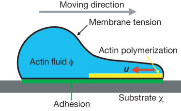
Figure 1: Schematic illustration of a model cell on a substrate. The cross-section of the cell is represented by a phase field $\phi$ while the substrate is defined by a field $\chi$. The dynamics of the cytoskeleton network is modeled as an actin fluid with velocity $\bf{u}$ (red arrow). Forces in the model include the membrane tension, cell-substrate adhesive forces, forces due to active actin polymerization, and cytosolic viscous forces (proportional to $\bf{u}$). Actin polymerization is restricted to a narrow region near the substrate at the cell front-half, as indicated by the yellow band. Additional model details are given in main text and in Supplemental Material.

II Results

II.1 Model

Our vertical cross-sectional model cell captures the interaction of the cell with the bottom and, possibly, top substrate, as well as the interior of the cell Tjhung et al. (2015) (Fig. 1). This is in contrast to most computational studies of cell motility which model a flat cell that is entirely in contact with the substrateStéphanou et al. (2008); Mogilner (2009); Buenemann et al. (2010); Alonso et al. (2018). This interior consists of a viscous cytoskeleton and is described as a compressible actin fluid Rubinstein et al. (2009) with constant viscosity while cell movement is driven by active stress, located at the front of the cell. Note that we do not consider myosin-based contraction. Furthermore, and following Ref. Rubinstein et al. (2009), we neglect the coupling between the actin fluid (representing the cytoskeleton) and the cytoplasm. The latter is assumed to be incompressible, resulting in volume conservation. This type of model which treats the cytoskeleton as an active viscous compressible fluid has been used in several recent studies Barnhart et al. (2011); Bois et al. (2011a); Shao et al. (2012); Camley et al. (2013); Goff et al. (2017). Friction is caused by the motion of the cytoskeleton relative to the substrate and is taken to be proportional to the actin fluid velocity. To accurately capture cell shape and its deformations, we use the phase field approach in which an auxiliary field $\phi(\boldsymbol{r},t)$ is introduced to distinguish between the interior ($\phi=1$) and exterior ($\phi=0$). This approach allows us to efficiently track the cell boundary which is determined by $\phi(\bm{r},t)=1/2$ Shao et al. (2010, 2012); Camley et al. (2013); Najem and Grant (2013); Ziebert and Aranson (2013); Alonso et al. (2018). In our model, boundary motion is driven by fluid flow which is determined by adhesion, friction, membrane forces and active protrusion. The cell is placed on a substrate which is parallel to the $x$ direction, and polarized in one direction. As described in earlier work Biben et al. (2005); Shao et al. (2012); Camley et al. (2013), the evolution of the cell’s shape is determined by the phase field dynamics:

$$\frac{\partial\phi(\bm{r},t)}{\partial t}=-\bm{u}\cdot\nabla\phi(\bm{r},t)+\Gamma(\epsilon\nabla^{2}\phi-G^{\prime}/\epsilon+c\epsilon|\nabla\phi|),$$ (1)

where the advection term couples the velocity field of the actin fluid, $\bm{u}$, to the phase field, $\epsilon$ is the width of the boundary, $\Gamma$ is a relaxation coefficient, $G$ is a double-well potential with minima at $\phi=1$ and $\phi=0$, and $c$ is the local curvature of the boundary (see Supplemental Material).

The actin fluid velocity field is determined by the stationary Stokes equation with an assumption of perfect compressibility (zero pressure and neglecting the inertial term because of low Reynolds number) Rubinstein et al. (2009); Bois et al. (2011b):

$$\nabla\cdot[\nu\phi(\nabla\bm{u}+\nabla\bm{u}^{T})]+\bm{F}_{sub}+\bm{F}_{mem}+\bm{F}_{area}+\nabla\cdot\sigma^{a}=0,$$ (2)

where $\nu$ is the viscosity of the cell and where $\sigma^{a}$ is the active stress due to actin polymerization, further detailed below. $\bm{F}_{sub}$ is the interaction between the cell and substrate and contains both adhesion and friction, $\bm{F}_{sub}=\bm{F}_{adh}+\bm{F}_{fric}$. The adhesive force is given by $\bm{F}_{adh}=\frac{\delta H(\phi,\chi)}{\delta\phi}\nabla\phi$, with the cell-substrate interaction potential:

$$H(\phi,\chi)=\int d\bm{r}^{2}\phi^{2}(\phi-2)^{2}W(\chi).$$

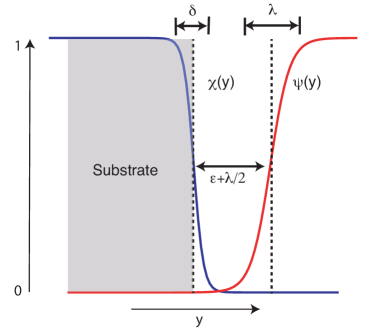
Figure S1: Illustration of the substrate field $\chi$, with width $\delta$, together with the protrusion band $\psi$, with width $\lambda$ and located a distance of $\epsilon$ away from the substrate.

Here, $\chi(\bm{r})$ is a constant field which marks the substrate (or ceiling) and continuously changes from $\chi=1$ (within the substrate) to $\chi=0$ (out of substrate; Fig. S1). $W(\chi)$ is a potential with a negative adhesion energy per unit length controlled by a parameter $A$ such that larger values of $A$ represent a larger adhesive force between cell and substrate. In addition, this potential contains a short-range repulsion that ensures that the cell does not penetrate the substrate. The term $\phi^{2}(\phi-2)^{2}$ is added to ensure that the force peaks within the boundary and vanishes at $\phi=0$ and $\phi=1$.

The second term in $\bm{F}_{sub}$ describes the frictional force between the cell and the substrate. Depending on the cell type, these forces can arise from focal adhesions or from non-specific cell-substrate interactions. For simplicity, the frictional force in our cross-sectional model is modeled as a viscous drag proportional to the actin fluid velocity :

$$\bm{F}_{fric}=-\xi_{s}\chi\bm{u}-\xi_{d}\bm{u},$$

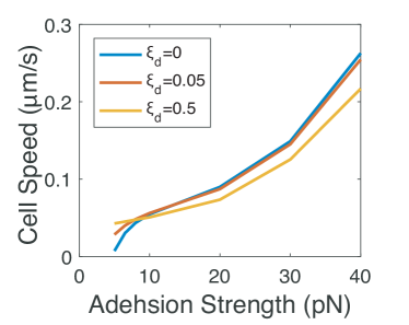
Figure S2: Cell speed as a function of adhesion strength for different values of the drag coefficient $\xi_{d}$ (in units of Pa s/$\mu$m). Cell speed changes little as $\xi_{d}$ is increased from 0 to 0.5.

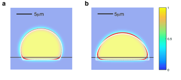
Figure S3: Simulation results of the phase-field method without active force (red line) compared to results obtained using Surface Evolver (white dots). The phase field is plotted using the indicated color scale. (a). Adhesion strength 10 pN. (b). Adhesion strength 20 pN.

where the first term is the cell-substrate friction, parameterized by the coefficient $\xi_{s}$, and the second term represents a damping force, introduced to increase numerical stability. We have verified that the cell speed changes little when we vary the drag coefficient $\xi_{d}$ (Fig. S2). Initially, we will vary both the adhesion energy (which controls spreading) and the frictional drag separately, allowing us to determine its relative contribution to cell motility. We will then examine model extensions which implement dependent adhesion and friction mechanisms (see Fig. 4). The uniform membrane tension $\bm{F}_{mem}$ and a force arising from cell area conservation $\bm{F}_{area}$ are introduced as in our previous work Shao et al. (2010); Camley et al. (2013). The latter force results in cell shapes with roughly constant area. More details of these forces, along with details of the simulation techniques for Eqns. (1&2) are given in Supplemental Material. As a consistency check, we have simulated cells without any propulsive force and have verified that the resulting static shapes agree well with shapes obtained using standard energy minimization simulations Brakke (1992) (Fig. S3).

Polarization in our model is introduced through the polarization indicator $\rho_{a}$ which is steering the actin polymerization. For simplicity, we have chosen $\rho_{a}=1$ at the front half and $\rho_{a}=0$ at the rear half of the cell. This corresponds to different actin promoter (e.g., Rac or Cdc42) distributions at the front and back induced by internal or external signaling. We assume the density of newly-made actin filaments is uniform at the cell membrane so we do not track the evolution of the actin density. In more complicated modelsShao et al. (2012); Camley et al. (2013) the actin can diffuse or be advected but we do not include them here to keep the model simple. Following earlier work Kruse et al. (2006); Nagel et al. (2014); Tjhung et al. (2015), we assume that protrusions that are generated by actin polymerization only occur at the front of the cell and close to the substrate. Our formulation of the active stress $\sigma^{a}$ incorporates these assumptions. Specifically, we introduce a field $\psi(\bm{r})$ with width $\lambda$ and located a distance $\epsilon$ away from the substrate (Fig. S1). By making the active stress proportional to $G(\psi)\phi\rho_{a}(\bm{r})$, we restrict possible protrusions to a narrow band parallel to the substrate and in the cell front. This band is schematically shown in yellow in Fig. 1. In addition, we localize the stress to the interface by multiplying the expression of $\sigma^{a}$ by the factor $|\nabla\phi|^{2}$. This is schematically shown as blue dots in Figs. 2 and 3. The expression for the stress is then given by:

$$\sigma^{a}=-\eta_{a}G(\psi)\phi\rho_{a}(\bm{r})\epsilon|\nabla\phi|^{2}\hat{\bm{n}}\hat{\bm{n}}.$$ (3)

Here, $\eta_{a}$ is the protrusion coefficient, and $\hat{\bm{n}}=\nabla\phi/|\nabla\phi|$ is the normal to the cell boundary. Note that our model does not include any possible feedback between substrate and stress generation.

Our simulations are carried out as described previously Camley et al. (2013) and further detailed in the Supplemental Material where we also list the full set of equations. As initial conditions, our simulations start with polarized cells in which the distribution of $\rho_{a}$ is asymmetric. The cell’s speed is tracked by $\bm{v}_{c}=d\bm{x}_{c}/dt$ with $\bm{x}_{c}$ the cell mass center $\bm{x}_{c}=\int\bm{x}\phi d^{2}\bm{r}/\int\phi d^{2}\bm{r}$ and simulations are continued until a steady state has been achieved. Parameters values used in the simulations are given in Table S1.

II.2 Simulation results and analysis

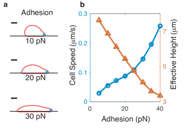
Figure 2: a, Cell shapes for different values of substrate adhesion strength. The blue dots here, and elsewhere, schematically indicate the location of active stress. Scale bar $5\mu m$. b, Cell speed (blue circles) and effective height of a cell (red triangles) as a function of the adhesion strength.

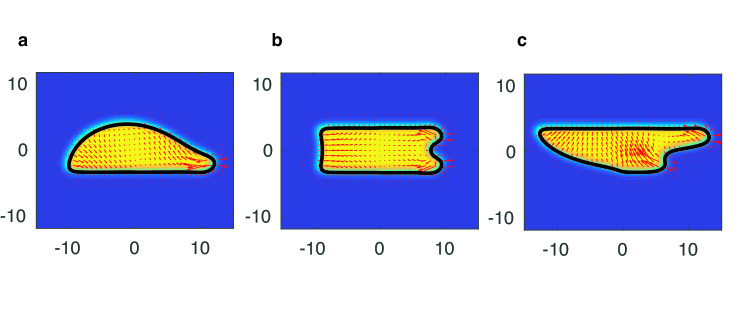
Figure S4: Numerical results showing the phase field using a color scale, the outline of the cell in black (defined as $\phi=1/2$), and the actin fluid velocity (multiplied with the phase field $\phi$) for a cell moving on a single substrate (a), and confined in a channel with equal (b) and unequal substrate adhesion (c). Arrows indicate the direction of the velocity and the arrow length indicates the amplitude of the velocity.

We first investigate how cells move on a single substrate with different adhesion energies. For this, we solve the phase field equations for different values of the adhesion parameter $A$. Examples of resulting cell shapes are shown in Fig. 2 while an example of the actin fluid velocity field is shown in Fig. S4. We find that with increasing adhesion strength, cells spread more and thus become thinner, similar to the spreading of a droplet on surfaces with increasing wettability (Fig. 2a). Our simulations reveal that the cell speed (i.e., the velocity parallel to the substrate) keeps increasing as the adhesion increases, without any indication of saturation (Fig. 2b). This is perhaps surprising, as our physical intuition suggests that adhesion and friction go hand in hand, with larger adhesion corresponding to higher friction. In our simulations, however, adhesion and friction are independent and can be separately adjusted.

To provide insights into the relation between adhesion, cell shape and speed, we consider a simplified version of Eq. (2), similar to the 1D model examined in Ref. Carlsson (2011). Since only asymmetric stress will contribute to the cell’s speed Tanimoto and Sano (2014), we only need to take into account the viscosity, friction and active stress in the equation:

$$\nu\nabla\cdot\sigma^{vis}-\xi\bm{u}+\nabla\cdot\sigma^{a}=0,$$ (4)

where $\sigma^{vis}=\nabla\bm{u}+\nabla\bm{u}^{T}$, $\xi$ is a friction coefficient taken to be spatially homogeneous, and $\sigma^{a}$ is the active stress which is 0 outside the cell. Boundary conditions include a steady cell shape $\hat{\bm{n}}\cdot\bm{v}_{c}=\hat{\bm{n}}\cdot\bm{u}$, zero net traction force $\int\xi\bm{u}d^{2}\bm{r}=0$, and zero parallel stress $\sigma^{vis}\cdot\hat{\bm{t}}=0$, where $\hat{\bm{n}},\hat{\bm{t}}$ are the normal and tangential unit vector, respectively.

It is in general not possible to solve Eq. 4 in a arbitrary geometry. However, for the special case of a fixed-shape rectangular cell with length $L$ and height $H$ occupying $x\in[-L/2,L/2],y\in[0,H]$ we can solve for the cell speed $v_{c}$ (see the Supplemental Material). By averaging the stress over the vertical direction and following Carlsson’s one-dimensional solution Carlsson (2011), we find:

$$v_{c}=-\frac{1}{4\nu H}\int_{-L/2}^{L/2}\frac{\tilde{\sigma}^{a}_{xx}\sinh(\kappa x)}{\sinh(\kappa L/2)}dx,$$ (5)

where $\kappa=\sqrt{\xi/(2\nu)}$ determines the spatial scale of the decay of a point stress source Carlsson (2011) and where $\tilde{\sigma}^{a}_{xx}=\int_{0}^{H}\sigma^{a}_{xx}dy$ (see also the Supplemental Material). From this solution it is clear that asymmetric active stress distribution will lead to cell motion. When $\kappa L/2\ll 1$, corresponding to a highly viscous cytoskeleton Bausch et al. (1998), the speed is proportional to the normalized active stress dipole $1/(LH)\times\int x\tilde{\sigma}_{xx}dx$. In the phase field model, the active stress in Eq. 3 is a negative bell shape function located at the front tip of the cell. This active stress can be approximated by $\tilde{\sigma}_{xx}=-\lambda\beta\delta[x-(L/2)_{-}]$ where $\beta$ is the active stress strength and where the stress is assumed to be located just inside the cell (see the Supplemental Material and Ref. Carlsson (2011)). Substituting this into Eq. 5, we find

$$v_{c}=\frac{\lambda\beta}{4\nu H},$$ (6)

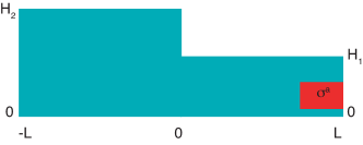
Figure S5: Schematic illustration of the non-deformable cell considered here, consisting of two rectangles of unequal height. Active stress occurs in the right (front) rectangle.

which shows that the cell speed scales inversely with the height of the cell, and that this scaling is independent of the cell length. Of course, a real cell will not be rectangular, and in the Supplemental Material we show that the cell speed scales with the average height for a more complex-shaped cell (Fig. S5). This suggests that the cell speed can be parameterized using an effective height $H_{\text{eff}}$, which can be computed by averaging the height over the cell length: $H_{\text{eff}}=(1/L)\int H(x)dx$. In Fig. 2b we see that $H_{\text{eff}}$ is monotonically decreasing when adhesion increases. The inverse relation between cell speed and effective height qualitatively agrees with the above analysis.

Interestingly, the above found relation between cell speed and cell height does not depend on the way the cell’s effective height is altered. To verify this, we also simulated cells in confined geometries in which they are “squeezed” between two substrates, as shown in Fig. 3a (an example of a cell with the actin fluid velocity field can be found in Fig. S4). Consistent with our analytical results, we find that as the chamber height is reduced, the cell’s speed increases while the cell’s effective height decreases (Fig. 3b). Furthermore, changing the adhesive strength on the top and bottom substrate while keeping the distance between them fixed will also affect the cell shape and its effective height (Fig. 3c and Fig. S4). Our simulations show that a difference in the top and bottom adhesion leads to an asymmetric cross-section and that the cell’s effective height reaches a maximum for equal top and bottom adhesion (Fig. 3d). Consistent with Eq. 6, our simulations show that the cell speed reach a minimum for substrates with equal adhesive strengths (Fig. 3d).

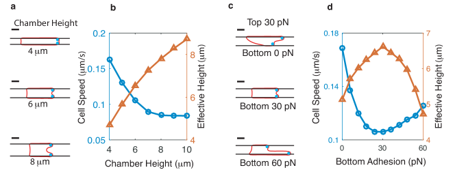
Figure 3: a. Cell shapes for different chamber heights. The adhesion strength of the top and bottom substrate is fixed at 30 pN. Scale bar: $5\mu m$. b. Corresponding cell speed (blue circles) and effective height (red triangles) as a function of chamber height. c. Cell shapes in a chamber with adhesive top and bottom substrates, with the top substrate adhesion fixed to 30 pN. Scale bar: $5\mu m$. d. Cell speed (blue circles) and effective height (red triangles) as a function of adhesion strength of the bottom substrate (chamber height=6$\mu$m).

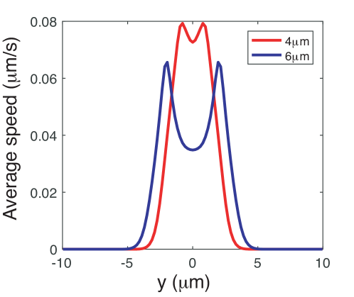
Figure S6: The average speed along the y-direction, defined as $1/L\int|\phi u_{x}|dx$, for a cell in a confined chamber with a height of $h=4\mu$m (red line) and $h=6\mu$m (blue line). The vertical shear dissipation increases with increasing cell height.

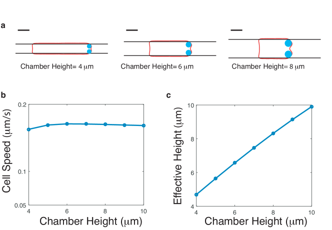
Figure S7: Simulation results of cells with a constant ratio 0.5 of the width of active stress band and the chamber height. The cyan dots schematically indicate the active stress sites. (a) Cell shapes for different chamber heights. Scalebar=5 $\mu m$ (b) Cell speed as a function of chamber height. (c) Effective height as a function of chamber height.

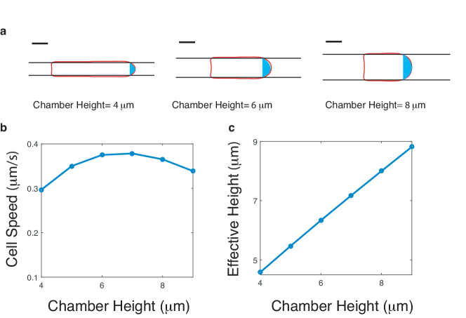
Figure S8: Simulation results of cells with active stress at the entire front, as indicated. (a) Cell shapes for different chamber heights. Scalebar=$5\mu$m (b) Cell speed as a function of chamber height. (c) Effective height as a function of chamber height.

Our results can be explained by realizing that cells contain a cytoskeleton network that can be described as a compressible viscous actin fluid. This actin fluid contains “active” regions which are confined to a layer with fixed width of $\lambda$, and “passive” regions that are outside these active regions. Active stress is only generated within this active region. Large viscosity will make the cell speed independent of cell length (see Eq. 5 and Ref. Carlsson (2011)). However, this viscosity also leads to dissipation due to internal shear stress: passive regions are coupled to the active regions through vertical shear interactions, resulting in dissipation. This dissipation increases with increasing cell height, as can also be seen in the velocity profile shown in Fig. S6, and thinner cells will move faster. We have tested this explanation by carrying out additional simulations. In one set, we simulated cells moving in chambers of varying height while keeping the ratio of the size of the active stress layer $\lambda$ and cell height constant. Consistent with our theoretical predictions, the speed of these cells is independent of the chamber height (Fig. S7). In addition, we have simulated cells in which the active stress region spans the entire front. Again in line with our theoretical insights, the cell speed was found to be largely independent of the chamber height (Fig. S8).

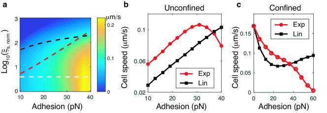
Figure 4: a, Cell crawling speed dependence on adhesion strength and friction coefficient (normalized by $\xi_{s}=$1 Pa s/$\mu$m). Cell speed is visualized using the colormap. The dashed lines correspond to different dependencies of the friction on adhesion (white: constant friction, black: linear dependence, red: exponential dependence). b, Cell speed for unconfined cells as a function of adhesion for linear (black line) and exponential (red line) dependence on adhesion (for parameters see main text). c, Speed of confined cells as function of bottom substrate adhesion strength for linear (black line) and exponential (red line) dependence of friction on adhesion (top substrate adhesion=30 pN, chamber height=6$\mu$m).

In our simulations, we have kept the friction coefficient constant and have thus ignored any potential link between adhesion and friction. This is likely appropriate for Dictyostelium cells but may not be valid for mammalian cells that have integrin mediated focal adhesions. The exact dependence of friction on adhesion is complicated and poorly understood Srinivasan and Walcott (2009); Walcott and Sun (2010). Our model, however, can easily be extended to explore the entire phase space of friction and adhesion. To illustrate this, we compute the speed of a cell crawling on a single substrate by sampling a broad range of adhesion strengths ($A=10$ pN to $A=40$ pN) and friction coefficients ($\xi_{s}=1$ Pa s/$\mu$m to $\xi_{s}=10^{3}$ Pa s/$\mu$m) while keeping all other parameters fixed. The resulting cell speeds are shown in Fig.4a using a color map. As expected, cells stall when adhesion is low and friction is high (dark blue region) while the highest cell speed occurs for large adhesion and a relatively broad range of low friction values (yellow region).

Different dependencies between friction and adhesion correspond to different trajectories through the two-dimensional phase space of Fig. 4a. The results we have presented so far correspond to traversing the phase space along the white dashed line in Fig. 4a. The black dashed line in this figure, on the other hand, represents a linear dependence between friction and adhesion ($\xi_{s}=\xi_{b}+\xi_{l}A/A_{l}$ with $\xi_{b}=$1 Pa s/$\mu$m, $\xi_{l}=$5 Pa s/$\mu$m, and $A_{l}=$1 pN) while the red dashed line represents an exponential dependence ($\xi_{s}=\xi_{b}+\xi_{e}\exp{(A/A_{e})}$ with $\xi_{b}=$1 Pa s/$\mu$m, $\xi_{e}=$1 Pa s/$\mu$m, and $A_{e}=$7 pN). For these two adhesion-friction dependencies, we have computed the cell speed for unconfined (Fig.4b) and confined cells (Fig.4c). For friction that depends linearly on adhesion, the speed of unconfined cells continues to increase as adhesion increases (black line in Fig.4b). This is very similar to the results we obtained for constant friction (cf. Fig. 2b). For exponential friction, the speed of unconfined cells initially increases for increasing adhesion. As adhesion increases, however, friction becomes more and more dominant, and cell’s speed reaches a maximum, followed by a decrease (red line in Fig.4b). This bi-phasic dependence of adhesion is consistent with a variety of experimentsHuttenlocher et al. (1996); Palecek et al. (1997); Gardel et al. (2008); Barnhart et al. (2011). For confined cells and a linear friction-adhesion relationship, the dependence of the cell speed on the adhesive strength of the bottom substrate is shown in Fig. 4.c (black line). Again, the results are very similar to our previously studied, constant friction case (cf. Fig.3d): cell speed reaches a minimum when the top and bottom adhesion strength are equal. Not surprisingly, the dependence of cell speed on bottom adhesion is different for the exponential relationship. Here, friction becomes dominant when adhesion increases, resulting in a cell speed that continuously decreases. These results show that friction plays a relatively small role in determining cell speed unless friction $\xi_{s}$ increases over orders of magnitude when adhesion $A$ changes by small amounts.

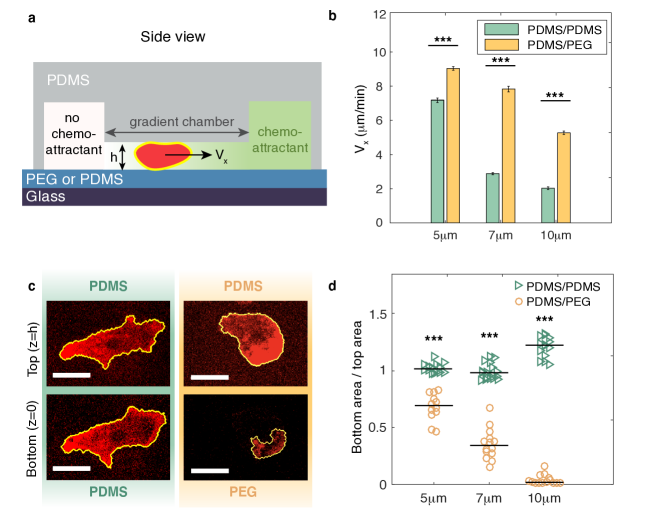
Figure 5: Experimental tests of the numerical and theoretical predictions. a. Schematic side view of the microfluidics chamber. Cells are placed in a confined chamber with variable height. The top substrate is composed of PDMS while the bottom substrate is either composed of PDMS or coated with less adhesive PEG. Cells are guided by a chemoattractant (cAMP) gradient of strength 0.45 nM/$\mu$m in the chamber. b. Cell speed in the gradient direction for varying chamber height, indicated along the x-axis, and top/bottom substrate composition, indicated by the label. For both PDMS/PDMS and PDMS/PEG substrate compositions, the cell speed decreases as chamber height is increased. Furthermore, for fixed chamber height, cells move faster when the bottom substrate is less adhesive (i.e., PDMS/PEG). P-value $<10^{-5}$ with unpaired t-test. Error bars represent the standard error of the mean. c. Scan of the cell area profile at the top and bottom of the chamber using the fluorescent membrane marker Car1-RFP ($h=5\mu$m). Cells with PEG-coated bottom substrates (PDMS/PEG) show asymmetric shapes whereas cells with PDMS bottom substrates (PDMS/PDMS) show symmetric shapes. Scale bar, 10$\mu$m. d. Ratio of top and bottom contact area under different conditions (label indicates bottom substrate composition). P-value $<10^{-5}$ with Wilcoxon rank-sum test.

II.3 Experimental results

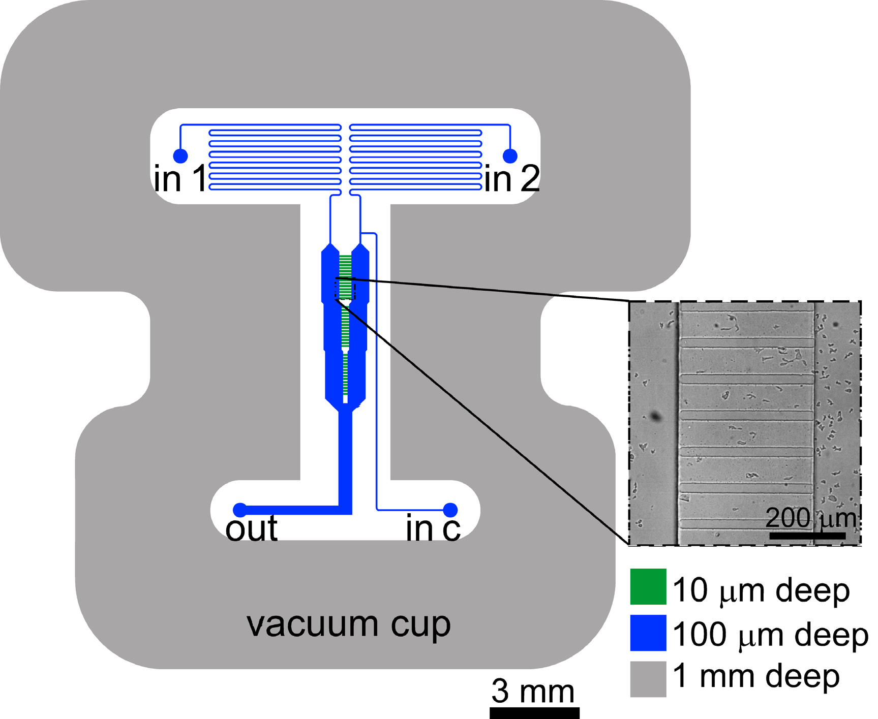
Figure S9: Design of the microfluidic device. The enlarged image is the experimental DIC view using a 10x objective showing gradient chambers and flow chambers with cells.

To test the above predictions, we performed motility experiments of Dictyostelium discoideum cells. Importantly, these cells, unlike mammalian cells, do not make integrin mediated focal adhesions and their substrate adhesion is likely to be mediated by direct physiochemical factors such as van der Waals attraction Loomis et al. (2012). Experiments are carried out in microfluidic devices, as shown in Fig. 5a and modified from earlier work Skoge et al. (2014) (see also Supplemental Material and Fig. S9). Cells are moving in chambers with height $h$ and with substrates that have variable adhesive properties. A constant cAMP gradient is established by diffusion so that cells preferably move in one direction (denoted as the $x$ direction). Note that the constant signal polarizing the cell in one direction is consistent with our model of a constantly-polarized cell.

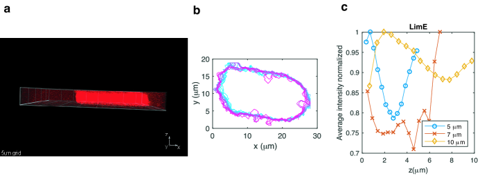
Figure S10: Experimentally obtained cell shapes and F-actin distribution for a cell moving in a 5 $\mu$m high channel. (a) z-stack of a cell containing the fluorescent membrane marker Car1-RFP. The cell extends from top to bottom PDMS substrate. (b) Cell outlines for different z values ranging from 0 (magenta) to 5 $\mu$m (cyan). The outline is essentially identical for all z values. (c) Average fluorescence intensity (normalized) of LimE, an F-actin marker, for each confocal slice as a function of z for representative cells in channels with height of 5,7 and 10 $\mu$m. All cells examined (N=5) displayed a qualitatively similar pattern with increased intensity close to the substrates.

Dictyostelium cells move by extending actin filled protrusions called pseudopods which can extend over a significant distance from the substrate. As a consequence, our confined cells occlude the entire space between two substrates. This was verified explicitly by labeling the cell with a fluorescent membrane marker and creating confocal z-stacks (Fig. S10). The results also demonstrate that in the case of symmetric adhesion the outline of the cell does not change appreciably as one moves from one to the other substrate. Furthermore, using LimE as a fluorescent marker, we have verified that the level of actin polymerization is largest near the substrates (Fig. S10 C). This observation is in agreement with earlier experiments of Dictyostelium cells migrating in a narrow channel Nagel et al. (2014) which revealed significantly larger levels of LimE fluoresence near the channel walls.

The top substrate of the chamber consists of Polydimethylsiloxane (PDMS) and the bottom substrate is either made of PDMS or is coated with a thin layer of Polyethylene glycol (PEG) gel. Cells moving on these PEG-coated substrates have vastly reduced adhesion, as reported in earlier studies Tzvetkova-Chevolleau et al. (2009). We measure the average speed of the cell $V_{x}$ in the direction of the chemoattractant gradient, both as a function of the height of the chamber and for different substrate compositions (Fig. 5b). Furthermore, to quantify the effect of the adhesive properties of the substrates on migrating cells, we measure the contact area of the cell on both top and bottom substrates of the chamber using confocal microscopy (Fig. 5c and d). More adhesive substrates will result in more cell spreading and thus larger contact areas.

Our theoretical predictions for cells in confinement are that decreased height increases speed, and that cells in asymmetric adhesion are faster than cells in symmetric adhesion. Both of these qualitative predictions are observed in our experiments. First, our experiments show that cell speed is significantly affected by the height of the chamber (Fig. 5b). Cells in chambers of height $h=10\mu$m move markedly slower than cells in chambers with $h=7\mu$m which, in turn, have smaller speed than cells in chambers with $h=5\mu$m. The trend of slower motion in deeper chambers holds for both PDMS and PEG coated bottom substrates. Furthermore, we have verified that these results do not depend on the steepness of the gradient (Fig. S11). These observations are fully consistent with our numerical and theoretical predictions (Fig. 3).

In addition, our experiments show that cells moving in a chamber with unequal top and bottom adhesion are markedly asymmetric (Fig. 5c), consistent with past results that showed that Dictyostelium cells only weakly adhere to PEG. Specifically, the contact area of cells on PEG coated substrates is significantly smaller than the contact area on PDMS substrates and the resulting asymmetry can be quantified by the ratio of bottom and top contact area. Cells with PDMS on top and bottom and for $h=$5$\mu$m and $h=$7$\mu$m have ratios close to 1 indicating that the shape is symmetric. In contrast, cells moving in chambers with these values of $h$ that have a PEG bottom have ratios that are much smaller than 1, indicating a more asymmetric cell shape. For the largest value of $h$ ($h=$10$\mu$m) cell preferentially attach to the top PDMS substrate, resulting in negligible contact area at the bottom PEG substrate and ratios close to 0. For this chamber height, the ratio for PDMS substrates is larger than one since cells are loaded on the bottom substrate and cannot fully attach to the top substrate.

Importantly, quantifying the cell speed for the different chambers reveals that cells in the symmetric PDMS/PDMS condition move slower than cells in the asymmetric PDMS/PEG condition (Fig. 5b). Again, these experimental results are fully consistent with our theoretical and numerical predictions and show that cell shape, and more specifically its effective height, can significantly affect motility speed (Fig. 3).

III Discussion and conclusion

In this study, we examined how cell shape can affect cell speed using simulations, analytics, and experiments. We should stress that our experiments can only be compared to the simulations on a qualitative level. Values for the model parameters are not precisely known, and our model cell is not fully three-dimensional. Nevertheless, separating the frictional and adhesive force in the model provides clear insights into the role of adhesion and cell shape in determining cell speed. This separation also makes it challenging to compare our results to previous studies that investigated the effects of cell-substrate interactions on cell speed. For example, a recent study using fish keratocyte cells Barnhart et al. (2011) found that cell spreading increases with adhesion strength (measured by the concentration of adhesive molecules). These experiments also revealed a biphasic speed dependence on adhesion such that cell speed increases between low and intermediate adhesion strengths and decreases between intermediate and high adhesion strengths. These results are similar to earlier experimental studies, and have previously been interpreted in terms of minimal models without cell shape DiMilla et al. (1991); Palecek et al. (1997); Liu et al. (2015). Our results suggest that the increase of cell speed with increased adhesion found in these experiments might be attributed to cell spreading and a lower effective height. The observed decrease in cell speed following a further increase in adhesion can then be explained by a larger relative role of frictional forces. Likewise, our experimental results suggest that our experiments operate in a regime where substrate friction is less important than the internal viscosity and hence the major effect of the substrate modification is the change in adhesion.

Our numerical and experimental results indicate that changing cell morphology through confinement can also significantly alter the migration speed, with decreasing chamber heights resulting in increased cell speeds. Comparison with other cell types is challenging as cells might change their behavior following confinement. A recent study using normal human dermal fibroblast cells, for example, found that slow mesenchymal cells can spontaneously switch to a fast amoeboid migration phenotype under confinement Liu et al. (2015). This phenotypic transition makes it difficult to directly compare those observations with our results and further investigation is needed to determine how different cell types behave in confinement.

We should point out that the simple scaling of cell speed dependence on cell height (Eq. 6) is based on the assumption of localized active stress (the numerator) and uniform cytoskeleton viscosity (the denominator) in the entire cross section. As shown in our experimental work and in previous studies Nagel et al. (2014), F-actin is localized close to the substrate, in support of the first assumption. It is currently unclear whether the second approximation is valid for Dictyostelium or other cells. Presumably, in cells with a clear segregation of actin cortex and cytoplasm, a large viscosity contrast could be present. Nevertheless, our arguments might still hold, as long as passive regions are coupled to the active regions through shear interactions (one example is the model in Ref.Kruse et al. (2006)). In this case, passive regions will still slow down the cell, but the relation between cell speed and shape will be more complicated and will have contributions from regions with different viscosity. To address this more general case, a full three-dimension model with viscosity contrast between the cortex and cytoplasm is necessary and will be part of future extensions.

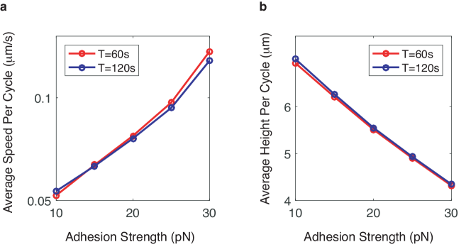
Figure S12: Cell speed and effective height for cells with oscillatory active stress. (a) Average cell speed, computed as moving distance divided by cycle time, and (b) effective height as a function of substrate adhesion strength. Shown are the results for oscillatory stress cycles with two different periods.

In summary, we show how adhesion forces result in cell spreading and that the accompanying shape changes can result in larger velocities. Key in this result is the existence of a narrow band of active stress that has a smaller spatial extent than the height of the cell. As a result, the dissipation due to the shear stress between this active band and the remainder of the cell increases as the effective height of the cell increases. In our model, we have assumed a cell motility model corresponding to stable flat protrusions. The conclusion that cell speed scales inversely with the effective height is also valid for other cell motility models as long as the active propulsion region has limited spatial extent. For example, replacing the constant active stress by an oscillating stress, similar to protrusion-retraction cycles seen in amoeboid cells, does not change the qualitative results (Fig. S12). Further extensions of our model could include focal adhesive complexes (to model a broader range of eukaryotic cell types) and different types of actin structures in different parts of the cell. These extensions can then be used to further determine the role of adhesion in cell motility.

Supplemental Material for “Cell Motility Dependence on Adhesive Wetting”

IV Phase field model of cell motility

The equations for the phase-field cross section model are:

$$\frac{\partial\phi(\bm{r},t)}{\partial t}=-\bm{u}\cdot\nabla\phi(\bm{r},t)+\Gamma(\epsilon\nabla^{2}\phi-G^{\prime}/\epsilon+c\epsilon|\nabla\phi|)$$ (S1)

$$\nabla\cdot[\nu\phi(\nabla\bm{u}+\nabla\bm{u}^{T})]+\bm{F}_{sub}+\bm{F}_{mem}+\bm{F}_{area}+\nabla\cdot\sigma^{a}=0.$$ (S2)

Here, $\phi$ describes the field of the cell. The double-well potential is defined as $G=18\phi^{2}(1-\phi)^{2}$ and the curvature is computed as $c=-\nabla\cdot(\nabla\phi/|\nabla\phi|)$ while $\Gamma$ is a relaxation coefficient. The force terms are explicitly explained below.

The substrate force contains the cell-substrate adhesion and friction: $\bm{F}_{sub}=\bm{F}_{adh}+\bm{F}_{fric}$, where

$$\bm{F}_{fric}=-\xi_{s}\chi\bm{u}-\xi_{d}\bm{u},\;\bm{F}_{adh}=\frac{\delta H(\phi,\chi)}{\delta\phi}\nabla\phi.$$

Here, $\bm{u}$ is the velocity field of the actin fluid and $\xi_{s},\xi_{d}$ are the cell-substrate friction coefficient and damping coefficient, respectively. $\chi$ is the field describing the substrate, and $H(\phi,\chi)$ is the interaction potential between the cell and substrate. The The cell moves either on top of a plain substrate or between a top and bottom substrate. The location of these substrates is given by a field $\chi(y)$ with a boundary width of $\delta$ (Fig. S1). Here, $\chi=1$ indicates the substrate into which the cell cannot penetrate, and $\chi=0$ indicates the region accessible to the cell. In our simulations, the substrate is parallel to the x direction and, for the case of a single substrate located at $y=y_{B}$, $\chi$ is written as

$$\chi(y)=\frac{1}{2}-\frac{1}{2}\tanh\{3(y-y_{B})/\delta\},$$

For a chamber with a parallel top substrate located at $y=y_{T}$ this becomes

$$\chi(y)=\frac{1}{2}+\frac{1}{2}\tanh\{3[|y-(y_{T}+y_{B})/2|-(y_{T}-y_{B})/2]/\delta\}.$$

Given $\phi$ and $\chi$, the interaction potential is:

$$H(\phi,\chi)=\int d\bm{r}^{2}\phi^{2}(\phi-2)^{2}W(\chi),$$

where $W(\chi)$ contains an attractive term, corresponding to adhesion, and a repulsive term, corresponding to the non-penetrability of the substrate. For the bottom substrate, we use

$$W(\chi)=-2A\frac{G(\chi)}{\delta}+\frac{g}{2}\chi(y+\epsilon),$$ (S3)

while the potential for the top substrate has an identical form with $\epsilon$ replaced by $-\epsilon$. Here, $A$ is the adhesion energy per unit length, $g$ is a parameter that measures the penalty of overlap between cell and substrate Camley et al. (2014), and $G$ is a double-well potential $G(\chi)=18\chi^{2}(1-\chi)^{2}$. The energy function

$$H(\phi,\chi)=\int\phi^{2}(\phi-2)^{2}W(\chi)d^{2}\bm{r}$$

corresponds, in the sharp interface limit, to an adhesive energy equal to $-Al$ where $l$ is the length of the cell in contact with the substrate. Note that the inclusion of the $\phi^{2}(\phi-2)^{2}$ results in a force that only vanishes outside the membrane Zhao et al. (2017). In our simulations we take $\delta=\epsilon/2$. For this choice of $\delta$ we simulated cells without any propulsive force. The resulting static shapes can be directly compared to standard energy minimization simulations. Fig. S3 shows that the phase field shapes agree well with shapes obtained using Surface Evolver, a simulation tool that evolves surfaces toward minimal energy by a gradient descent method Brakke (1992).

The contribution from both the tension and bending of the membrane is captured by $\bm{F}_{mem}$. In our simulation we ignore the bending term since it contributes little to the shape of cell. The tension energy is given by Shao et al. (2010); Camley et al. (2013):

$$H_{ten}=\int\frac{\gamma}{2}[\epsilon|\nabla\phi|^{2}+\frac{G(\phi)}{\epsilon}]d^{2}\bm{r},$$

resulting in $\bm{F}_{mem}=\frac{\delta H_{ten}}{\delta\phi}\nabla\phi$. Area conservation is introduced via $\bm{F}_{area}=M_{a}(\int\phi d\bm{r}^{2}-A_{0})\nabla\phi$ with $A_{0}$ the prescribed area size, and $M_{a}$ a parameter which controls the strength of the area constraint Shao et al. (2010).

The active stress term in our model, $\sigma^{a}=-\eta_{a}G(\psi)\phi\rho_{a}\epsilon|\nabla\phi|^{2}\hat{\bm{n}}\hat{\bm{n}}$, is similar to our earlier work Shao et al. (2012) but only acts near the substrate. This is accomplished through the addition of the term $G(\psi)=18\psi^{2}(1-\psi)^{2}$, where $\psi$, for the bottom substrate, takes on the form

$$\psi_{B}(y)=\frac{1}{2}+\frac{1}{2}\tanh\{3[y_{B}+(\epsilon+\lambda/2)-y]/\lambda\}.$$

A similar expression is used for the top substrate. The inclusion of $G(\psi)$ results in active stresses confined to a band with width $\lambda$ and located a distance $\epsilon$ away from the substrate (Fig. S1). Note that vertical height of the active stress is controlled by $\lambda$ and that $\int G(\psi)dy=\lambda/2$.

Three examples of the velocity fields obtained numerically are shown in Fig. S4, corresponding to the cell motion on single substrate, confined in channels and confined in channels with asymmetric adhesion (Fig. 2 and Fig. 3 in main text). The retrograde flow patterns are similar to previous studies inShao et al. (2012).

V Numerical Methods

The equation for $\phi$ is stepped by uniform time step $\Delta t=2\times 10^{-3}s$ in a forward Euler scheme so that $\phi$ at time step $n+1$ is obtained from $\phi$ at time step $n$:

$$\phi^{(n+1)}=\phi^{(n)}-\Delta t\bm{u}+\Delta t\Gamma[\epsilon\nabla^{2}\phi^{(n)}-G^{\prime}(\phi^{(n)})+\epsilon c^{(n)}|\nabla\phi^{(n)}|],$$

Here, $c^{(n)}=-\nabla\cdot(\nabla\phi^{(n)}/|\nabla\phi^{(n)}|)$ is computed using a finite difference method and all other differentiation operators are computed using a fast Fourier spectral method. Simulations were carried out on a $256\times 256$ grid of size $50\mu m\times 50\mu m$. Model parameters, modified from Shao et al. (2012); Camley et al. (2013), are listed in Table S1.

The velocity field $\bm{u}$ is updated every time step by a semi-implicit Fourier spectral method after updating $\phi$ as detailed in Camley et al. (2013). The equation is iterated as:

$$\xi_{0}\bm{u}_{k+1}-\nu\tilde{\phi}\nabla^{2}\bm{u}_{k+1}=\nabla\cdot[\nu\phi\nabla\bm{u}_{k}+\nu(\phi-\tilde{\phi})\nabla\bm{u}^{T}_{k}]-\xi_{s}\chi\bm{u}_{k}+\bm{F},$$

where $\tilde{\phi}=2$, and $\bm{F}$ represents the terms in the Stokes equation that are independent of the iteration step $k$. The iteration will continue until

$$\frac{\max|\bm{u}_{k+1}-\bm{u}_{k}|}{\max|\bm{u}_{k}|}<0.1,$$

or until a maximal number of iterations (here chosen to be 20) is reached.

VI Analytical Results

As stated in the main text, we aim to analytically solve Eq. S1&S2, where several simplifications have to be made. First, we are trying to find the steady-state solutions, so the cell shape will not change with time. Thus we drop Eq. S1 and, instead, put boundary conditions for Eq. S2. In accordance with our simulations, we choose slip boundary conditions, similar toCarlsson (2011). The boundary condition for the steady-state cell shape is

$$\bm{u}\cdot\hat{\bm{n}}=\vec{v}_{c}\cdot\hat{\bm{n}},$$

where $\vec{v}_{c}$ is the cell’s mass of center velocity, which is our target to solve, and $\hat{\bm{n}}$ is the normal unit vector of the boundary. The cell’s boundary is free so the parallel stress at the boundary is zero

$$\hat{\bm{t}}\cdot\sigma^{vis}=0,$$

where $\hat{\bm{t}}$ is the tangential unit vector of the boundary. Notice that the active stress is always constrained inside the cell so it will not enter any boundary conditions. The total force of the cell exerted on substrate should be balanced which gives a zero net traction force condition

$$\int\xi(\bm{r})\bm{u}d^{2}\bm{r}=0,$$

where $\xi(\bm{r})$ is the friction coefficient at different locations. To get analytical expressions, we neglect the spatial heterogeneity in friction and simply take $\xi(\bm{r})=\xi$. This simplification does not change the central feature of our main result (the cell’s speed is inversely related to the cell’s height).

Second, we only take into account the viscosity, friction and active stress because they are directly related to the cell motion. The adhesion, area conservation and membrane forces only contribute to the cell’s shape, which is implicitly included in the boundary conditions. Thus we get a simplified equation for Eq. S2:

$$\nu\nabla\cdot\sigma^{vis}-\xi\bm{u}+\nabla\cdot\sigma^{a}=0.$$ (S4)

Integrating the above equation and using the zero traction force condition, we obtain $\oint(\nu\sigma^{vis}+\sigma^{a})\cdot\hat{\bm{n}}dl=0$. As the active stress $\sigma^{a}$ is constrained inside the cell, this will lead to a condition equivalent to the zero traction force condition

$$\oint\hat{\bm{n}}\cdot\sigma^{vis}dl=0,$$

which is the zero traction force condition we used below.

Notice that a fixed cell shape has to be given in order to apply the boundary conditions. Since we only care about the cell’s mass of center velocity $\vec{v}_{c}$, and not the full solution for $\bm{u}$, we will next show how $\vec{v}_{c}$ can be obtained without knowing $\bm{u}$.

VI.1 Analytical solution of the rectangular model cell

Here we wish to solve the Eq. S4 for a rectangular fixed cell shape $x\in[-L/2,L/2],y\in[0,H]$ with an unknown cell speed $v_{c}$ (notice we put the x-direction as cell moving direction so $v_{c}$ is a scalar). The boundary conditions are $\bm{u}_{x}(x=\pm L/2)=v_{c},\;\bm{u}_{y}(y=0,H)=0,\;\rm{and}\int\bm{u}dxdy=0$. Integrating the Stokes equation, we get $\int d^{2}\bm{r}(\nu\nabla\cdot\sigma^{vis}+\nabla\cdot\sigma^{a})=\oint(\nu\sigma^{vis}\cdot\bm{n}+\sigma^{a}\cdot\bm{n})dl=\xi\int\bm{u}d^{2}\bm{r}=0$. Note that the active stress $\sigma^{a}$ should be constrained within the cell Carlsson (2011) resulting in the zero net traction force condition $\oint\sigma^{vis}\cdot\bm{n}dl=0$. This means $\int[\sigma_{xx}^{vis}(x=L/2)-\sigma_{xx}^{vis}(x=-L/2)]dy=\int[\partial_{x}\bm{u}_{x}|_{x=L/2}-\partial_{x}\bm{u}_{x}|_{x=-L/2}]dy=0$ and $\int[\sigma_{xy}^{vis}(y=H)-\sigma_{xy}^{vis}(y=0)]dx=0$ due to the rectangular shape.

The tangential vector $\hat{\bm{t}}$ can be determined by the normal vector $\hat{\bm{t}}_{x}=-\hat{\bm{n}}_{y},\hat{\bm{t}}_{y}=\hat{\bm{n}}_{x}$. The zero-parallel stress condition $\hat{\bm{t}}\cdot\sigma^{vis}=0$ results in

$$\hat{\bm{n}}_{y}\sigma^{vis}_{xx}-\hat{\bm{n}}_{x}\sigma^{vis}_{xy}=0,\;\;\hat{\bm{n}}_{y}\sigma^{vis}_{xy}-\hat{\bm{n}}_{x}\sigma^{vis}_{yy}=0.$$

For rectangular boundaries, these conditions lead to

$$\sigma^{vis}_{xy}=0,$$ (S5)

at all boundaries.

Since the cell is moving along x-direction, only $\bm{u}_{x}$ is relevant and we can integrate the 2D Stokes equation in the y-direction. With the condition of $\sigma^{vis}_{xy}=0$, we obtain a 1D Stokes equation:

$$2\nu\frac{\partial^{2}\tilde{\bm{u}}_{x}}{\partial x^{2}}-\xi\tilde{\bm{u}}_{x}+\frac{\partial\tilde{\sigma}^{a}_{xx}}{\partial x}=0,$$ (S6)

where $\tilde{\bm{u}}_{x}=\int_{0}^{H}\bm{u}_{x}dy$, and $\tilde{\sigma}^{a}_{xx}=\int_{0}^{H}\sigma^{a}_{xx}dy$. The corresponding boundary conditions are $\tilde{\bm{u}}_{x}(L/2)=\tilde{\bm{u}}_{x}(-L/2)=v_{c}H$ and $\partial_{x}\tilde{\bm{u}}_{x}|_{x=L/2}=\partial_{x}\tilde{\bm{u}}_{x}|_{x=-L/2}$. This is exactly the same problem as in reference Carlsson (2011). Using standard Green’s function methods, we obtain:

$$\tilde{\bm{u}}_{x}(L/2)=-\frac{1}{4\nu}\int_{-L/2}^{L/2}\frac{\tilde{\sigma}^{a}_{xx}\sinh(\kappa x)}{\sinh(\kappa L/2)}dx,$$

and, since $\bm{u}_{x}=v_{c}$ at boundaries $x=\pm L/2$, we obtain

$$v_{c}=\frac{\tilde{\bm{u}}_{x}(L/2)}{H},$$ (S7)

as reported in the main text (Eq. 5). If the active stress is confined in a band with width $\lambda$, i.e., $\int_{0}^{H}\sigma^{a}_{xx}dy=\lambda f(x)$, the cell’s speed $v_{c}$ will scale as:

$$v_{c}=\frac{\lambda v_{0}}{H},$$ (S8)

where $v_{0}$ is a constant, corresponding to the boundary velocity determined by the 1D problem $2\nu\partial_{x}^{2}v-\xi v+f^{\prime}(x)=0$ with homogeneous boundary conditions. Notice that this scaling does not depend on the vertical position of the active stress. Therefore, our model will give the same cell speed independent of the type of active stress (actin polymerization, myosin contraction), as long as the integrated active stress is the same.

VI.2 Effective height for non-rectangular cells

In the above section, the speed of a rectangular cell was determined exactly. Actual cells are, of course, not rectangular but obtaining a solution for cells with more complex shapes is challenging. Nevertheless, insight can be obtained by considering a cell composed of two rectangles, one positioned at $[-L,0]\times[0,H_{2}]$ and one positioned at $(0,L]\times[0,H_{1}]$ ($H_{1}<H_{2}$ (see Fig. S5). We take the active stress to be located at the latter (right) rectangle. This problem has the same boundary conditions as above, with two additional continuity conditions:

$$\bm{u}_{x}(x=0^{+})=\bm{u}_{x}(x=0^{-}),\;\;\;\partial_{x}\bm{u}_{x}|_{x=0^{+}}=\partial_{x}\bm{u}_{x}|_{x=0^{-}}.$$ (S9)

To simplify the problem, we introduce the new variables $u_{1}=\int_{0}^{H_{1}}\bm{u}_{x}dy$ and $u_{2}=\int_{0}^{H_{2}}\bm{u}_{x}dy$. Using the continuity condition we have:

$$u_{2}(0^{-})=\int_{0}^{H_{2}}\bm{u}_{x}(x=0^{-})dy=\int_{H_{1}}^{H_{2}}\bm{u}_{x}(x=0^{-})dy+\int_{0}^{H_{1}}\bm{u}_{x}(x=0^{+})dy=(H_{2}-H_{1})v_{c}+u_{1}(0^{+}).$$

Together with $u_{1}(L)=H_{1}v_{c},\,u_{2}(-L)=H_{2}v_{c}$ we get

$$\left.u_{2}\right|_{-L}^{0}+\left.u_{1}\right|_{0}^{L}=0.$$ (S10)

The zero traction force will give

$$\int_{0}^{H_{2}}\partial_{x}\bm{u}_{x}|_{x=-L}dy=\int_{H_{1}}^{H_{2}}\partial_{x}\bm{u}_{x}|_{x=0}dy+\int_{0}^{H_{1}}\partial_{x}\bm{u}_{x}|_{x=L}dy.$$

Combining with the stress continuity we obtain

$$\partial_{x}u_{2}|_{0}=\int_{0}^{H_{2}}\partial_{x}\bm{u}_{x}|_{x=0}dy=(\int_{0}^{H_{1}}dy+\int_{H_{1}}^{H_{2}}dy)(\partial_{x}\bm{u}_{x}|_{x=0})=\partial_{x}u_{1}|_{0}+\partial_{x}u_{2}|_{-L}-\partial_{x}u_{1}|_{L}.$$

such that

$$\left.\partial_{x}u_{2}\right|_{-L}^{0}+\left.\partial_{x}u_{1}\right|_{0}^{L}=0.$$ (S11)

Notice that Eq. S10 and Eq. S11 have clear physical meanings, namely flow conservation and force balance, respectively. It is convenient to introduce the net flow $C$ and net force $F$ on each rectangle:

$$u_{2}|_{-L}^{0}=C,\;\;u_{1}|_{0}^{L}=-C,\;\;\partial_{x}u_{2}|_{-L}^{0}=F,\;\;\partial_{x}u_{1}|_{0}^{L}=-F,$$

and, using the zero-parallel stress condition, we obtain the 1D version of the problem for the right and left rectangle:

$$2\nu\partial_{x}^{2}u_{2}-\xi u_{2}=0,\;\;\;2\nu\partial_{x}^{2}u_{1}-\xi u_{1}+\partial_{x}\sigma^{a}=0,$$

with $\sigma^{a}=\int_{0}^{H_{1}}\sigma_{xx}dy$. $u_{1}$ can be solved by superposition of two parts: $\tilde{u}_{1}$ with homogeneous boundary conditions and active stress, and $\hat{u}_{1}$ with inhomogeneous boundary conditions but zero active stress. After substituting $u_{1}=\tilde{u}_{1}+\hat{u}_{1}$, we obtain

$$2\nu\partial_{x}^{2}\tilde{u}_{1}-\xi\tilde{u}_{1}+\partial_{x}\sigma^{a}=0,\;\tilde{u}_{1}|_{0}^{L}=0,\;\partial_{x}\tilde{u}_{1}|_{0}^{L}=0,$$

and

$$2\nu\partial_{x}^{2}\hat{u}_{1}-\xi\hat{u}_{1}=0,\;\hat{u}_{1}|_{0}^{L}=-C,\;\partial_{x}\hat{u}_{1}|_{0}^{L}=-F.$$

We can then solve for $\tilde{u}_{1},\hat{u}_{1}$ and $u_{2}$ and obtain the boundary velocity:

$$H_{1}v_{c}=u_{1}(L)=v_{a}-\frac{C}{2}-\frac{\alpha F}{2\kappa},\;\;H_{2}v_{c}=u_{2}(-L)=-\frac{C}{2}+\frac{\alpha F}{2\kappa},$$ (S12)

and the boundary stresses:

$$\partial_{x}u_{2}|_{-L}=-\frac{F}{2}+\frac{\alpha\kappa C}{2},\partial_{x}u_{2}|_{0}=\frac{F}{2}+\frac{\alpha\kappa C}{2},\partial_{x}u_{1}|_{0}=\pi_{a}+\frac{F}{2}-\frac{\alpha\kappa C}{2},\partial_{x}u_{1}|_{L}=\pi_{a}-\frac{F}{2}-\frac{\alpha\kappa C}{2},$$ (S13)

where $\kappa=\sqrt{\xi/2\nu},\alpha=\coth(\kappa L/2)$. $v_{a}$ and $\pi_{a}$ are the boundary speed and boundary stress from the homogeneous equation of $\tilde{u}_{1}$, which are constants.

To calculate $v_{c}$, we have to determine $C$ and $F$. Eq. S12 gives one condition $H_{1}/H_{2}=u_{1}(L)/u_{2}(L)$ and an additional condition from the stresses in Eq. S13 is needed. Unfortunately, there is no simple relation between the four equalities in Eq. S13 since the stress continuity equation cannot be defined at the boundary at $x=0$ and between $y=H_{1}$ and $y=H_{2}$. Instead, we assume that the ratio of the integrated stress at $x=0$ satisfies $(\partial_{x}u_{1}|_{0})/(\partial_{x}u_{2}|_{0})=\beta$. Then, we have:

$$v_{c}=\frac{\kappa v_{a}\alpha^{2}(1+\beta)+\kappa v_{a}(1-\beta)-2\alpha\pi_{a}}{\kappa[\alpha^{2}(1+\beta)(H_{1}+H_{2})+(\beta-1)(H_{1}-H_{2})]}.$$ (S14)

Note that when $H_{1}=H_{2}$, corresponding to $\beta=1$, this result gives the same scaling as for the simple rectangular shape.

With $\alpha\gg 1$, corresponding to a highly viscous cytoskeleton, we have

$$v_{c}\approx\frac{v_{a}}{H_{1}+H_{2}}-\frac{2\pi_{a}}{\kappa\alpha(1+\beta)(H_{1}+H_{2})},$$ (S15)

which clearly shows that the cell speed is scaling inversely with the average height $(H_{1}+H_{2})/2$.

VII Test of model predictions

The above analysis indicates that the ratio of the height of stress band $\lambda$ and the cell height $H$ determines the cell speed. Thus, cells with equal ratio should have similar speeds. To test this explicitly, we simulated cells in chambers with heights varying between $h=4\mu m$ and $h=10\mu m$, constraining the cell’s height, while keeping the ratio $\lambda/h=0.5$. Cells shapes for three different chamber heights are shown in Fig. S7a while the cell speed and effective height as a function of chamber height are shown in Fig. S7b and c, respectively. Clearly, the results from Fig. S7b show that the speed of the cell is independent of the chamber height, consistent with our model prediction.

In addition, our derived expression predicts that if $\lambda=H$, corresponding to an active stress region that spans the entire height of the cell, the cell speed should be independent of the chamber height. To verify this, we performed simulations of confined cells with the active stress at the entire cell front. To this end, we no longer constrain the stress to a narrow band and, instead, use $\sigma^{a}=-\phi\rho_{a}(1-\chi)\epsilon|\nabla\phi|^{2}\hat{\bm{n}}\hat{\bm{n}}$. We introduce the factor of $1-\chi$ to prevent protrusion in the region where the cell and substrate overlap, something that is excluded from occurring in other models when the band restricts protrusion. Resulting cell shapes for different chamber heights are shown in Fig. S8a. In Fig. S8b, we plot the cell speed as a function of the chamber height and in the Fig. S8 we plot the effective height. As expected, the cell speed changes little as the chamber height is varied, again consistent with our predictions.

VIII Oscillatory protrusions

Results in the main text are for cells with constant active stress, resulting in constant cell shapes. Such constant shapes are applicable to fish keratocytes, fast moving cells that maintain their morphology Keren et al. (2008). Other cell types, however, including neutrophils and Dictyostelium discoideum cells Levine and Rappel (2013), move in a more time-dependent way, with repetitive and short-lived protrusions called pseudopods. To determine the dependence of cell speed on chamber height for these types of cells we introduce an oscillatory modulation to the active stress: $\sigma^{a}=-\phi\rho_{a}G(\psi)\sin(2\pi t/T)\epsilon|\nabla\phi|^{2}\hat{\bm{n}}\hat{\bm{n}}$. Here, $T$ is the period of the oscillation cycle which can be varied. Results from additional simulations show that the cell speed gets larger as the substrate adhesion is increased (Fig. S12a). This dependence on adhesion was found to be largely independent of the period and is similar to the one found for model cells with constant stress (Fig. 2b). Also consistent with our results in the main text (Fig. 2c), the effective height is again inversely related to the adhesion strength.

IX Experiments

IX.1 Cell culture and preparation

Wild type Dictyostelium discoideum (AX4) cells were transformed with a construct in which the regulatory region of actin 15 drives genes encoding a fusion of GFP to LimE ($\Delta$ coil LimE-GFP) and a gene encoding a fusion of RFP to Coronin (LimE GFP/corA RFP)Fuller et al. (2010). Cells were transformed with the plasmid pDM115 cAR1-RFP (Hygromycin resistance) to visualize the membrane. Cells were grown in a shaker, containing 35.5g HL5 media (^®FORMEDIUM)/L of DI waterSussman (1987) in a shaker. When cells reached their exponential phase ($1-2\times 10^{6}$ cells/mL), they were harvested by centrifugation, washed in $\text{KN}_{2}$/Ca buffer (14.6 mM $\text{KH}_{2}\text{PO}_{4}$, 5.4 mM $\text{Na}_{2}\text{HPO}_{4}$, 100 $\mu$M $\text{CaCl}_{2}$, pH 6.4), and resuspended in $\text{KN}_{2}$/Ca at $10^{7}$ cells/mL. The washed cells were developed for 5h with pulses of 50 nM cAMP added every 6 min.

IX.2 Microfluidic device

The design of microfluidic device used in the study is similar to the design of the devices that were previously used to study gradient sensing in yeastPaliwal et al. (2007) and chemotaxis in DictyosteliumSkoge et al. (2010, 2014). The microfluidic device (Fig. S9) consists of a lithographically fabricated silicone (polydimethylsiloxane, PDMS, Sylgard 184) chip and a cover glass substrate (with either PDMS or hydrogel coating, see below), against which the chip is sealed using vacuum suction. To this end, the network of liquid-filled microfabricated microchannels of the chip, which are relatively narrow and either 100 or 10 $\mu$m deep, is surrounded by a wide ($\sim$6 mm) and deep ($\sim$1 mm) groove, serving as a vacuum cup. When the PDMS chip is placed on a substrate, the application of vacuum to the cup generates a pulling force that instantly seals the liquid-filled microchannels of the chip against the substrate. The application of vacuum also leads to controlled partial collapse of the microchannels, making it possible to reduce the depth of the 10 $\mu$m deep microchannels by $>5\mu$m by controlling the level of vacuum. The network of liquid-filled microchannels of the device (Fig. S9) has a single outlet (out), two main inlets, for a $C_{0}=$100nM solution of cAMP (in 1) and for buffer (in 2), and an auxiliary inlet for cell loading (in c). The functional region of the device has two mirror-symmetric 100 $\mu$m deep, 500 $\mu$m wide flow-through channels (Fig. S9), which are connected to the two main inlets and are flanking 3 clusters of 10 $\mu$m deep gradient chambers. The flow through the device is driven by applying equal differential pressures of $\sim$2 kPa between the two main inlets and the outlet. The resulting mean flow velocity in the 500 $\mu$m wide flow-through channels is $\sim$200 $\mu$m/s. The gradient chambers are all 70 $\mu$m wide and each cluster has 15 identical chambers with equal lengths. The lengths $L$ of the gradient chambers in the upstream, middle, and downstream clusters are 360, 220, or 120 $\mu$m, respectively. There is practically no flow through the gradient chamber because of near zero pressure gradient along them, and the diffusion of cAMP from the flow-through channel perfused with the 100 nM solution to the flow-through channel perfused with buffer results in linear concentration profiles of cAMP with gradients of 0.28, 0.45, and 0.83 nM/$\mu$m, respectively. In different sets of experiments, the application of different levels of vacuum resulted in the effective depths of the gradient chambers of 10, 7, and 5 $\mu$m.

IX.3 Substrate preparation

In our experiments, the microfluidic chips were sealed against cover glass substrates with two different types of coating: $\sim$10 $\mu$m thick layer of PDMS of the same type as the material of the chip and $\sim$3 $\mu$m thick layer of 30% polyethylene glycol (PEG) gel. In the former case, the cover glass was a #1.5 thickness 47 mm circle at the bottom of a 50 mm WillCo cell culture dish. A small amount ($\sim$0.2 mL) of PDMS pre-polymer (10:1 mixture of base and curing agent of Sylgard 184 by Dow Corning) was dispensed onto the cover glass. Spin-coating was made at 6000 rpm for 2 min, and PDMS was cured by overnight baking in a 60$\mathrm{\SIUnitSymbolDegree}$C oven. In the latter case, the cover glass was #2, 50x35 mm rectangle. The cover glass was cleaned with water and ethanol, dried, air-plasma treated for 10 s, and then exposed to 3-(Trimethoxysilyl) propyl Methacrylate (^®Aldrich) vapor at 75$\mathrm{\SIUnitSymbolDegree}$C for 30 min. A 30% PEG pre-polymer solution was prepared by mixing PEG diacrylate (PEG-DA; avg Mn 900, ^®Aldrich) with a 0.03% aqueous solution VA086 (300 $\mu$g dissolved in 1000 $\mu$L of DI water) in a 3:7 ratio by volume. VA086 is iLine (365nm) sensitive UV photo-initiator that cross-links PEG-DA molecules (thus, converting a PEG-DA solution into a PEG gel) by binding to the acrylate groups and also links PEG-DA chains to the acrylate groups on the glass surface. An $\sim$100$\mu$L drop of the solution was dispensed onto the center of the cover glass and squeezed to a thin layer by placing an untreated #1.5 thickness, 30 mm diameter round cover glass on top, gently pushing this second cover glass with a pipette tip, and removing the excess solution with a wipe. The cross-linking of PEG-DA was done by exposing it to a total of 2.19 $J/cm^{2}$ of 365 nm UV (derived from 365nm UV LEDs; $\sim$365 $mW/cm^{2}$ for 60 sec). After the round cover glass was removed, the 50x35 mm cover glass had an $\sim$4 $\mu$m thick layer of covalently bonded PEG gel in the middle.

IX.4 Data acquisition and image analysis

Differential interference contrast (DIC) images were taken of all gradient chambers on a spinning-disk confocal Zeiss Axio Observer inverted microscope using a 10x objective and a Roper Cascade QuantEM 512SC camera. DIC images were captured every 15 s for 30 min and were used to calculate the speed of the cells. To obtain the shape of the cells, fluorescent images (488 nm and 561 nm excitation) were captured every 2 seconds with a 63X oil objective. To visualize the shape of the cells near the substrates, z-stacks of confocal images were collected.

The centroids of all cells were tracked across the gradient chambers from 10X image sequences using Slidebook 6 (Intelligent Imaging Innovations) software. Cells that moved more than 5 frames without encountering another cell were chosen for data analysis. 50 to 100 cell tracks were analyzed in each experiment. Velocity in the gradient direction, $V_{x}(t)$, was computed using data from frames 45 s apart with Matlab R2016a (The MathWorks, Natick, MA). We have verified that cell speeds were largely independent of their positions within the gradient chambers. Consequently, the average speed was defined as the mean speed of all cells at least 30$\mu$m from the sides of the chamber adjacent to the flow-through channels at all recorded times.

Cells outlines near the top (PDMS chip) and the bottom (substrate, PDMS or PEG) of the gradient chambers were obtained from confocal fluorescence images at 63X magnification with a custom-made Matlab code, as follows. After removing the average background intensity value, images were binarized using a threshold that was dependent on the cell’s maximum intensity. Matlab algorithms were then used to dilate images, to fill possible holes, to erode images, to smooth images, and to provide information (area and outlines) about the connected pixels of the binary image. Finally, using the resulting images, we computed the ratio between the cell contact area at the top and bottom of the chamber and averaged this ratio over three time points for each cell.

IX.5 Statistics and reproducibility

Each experiment was carried out four or five times on different days and the data were averaged for N=200-300 cells. Cell speed was found to be approximately normally distributed and p-values were computed with the unpaired t-test. For the area size ratio, the data distribution was not normal, and the Wilcoxon rank-sum test was used to obtain the p-values. The variations of the cell speed with the gradient chamber height and the type of substrate coating (PDMS vs. PEG) followed the same trends in gradient chambers of different lengths, $L$ (cf. Fig. 4d and Fig. S11).

Parameter	Description	Value
$\gamma$	Tension	20 pN
$\epsilon$	Width of phase field	2 $\mu$m
$A_{0}$	Cell area size	120 $\mu\text{m}^{2}$
$M_{a}$	Cell area conservation strength	$20\;\text{pN}/\mu m$
$\Gamma$	Phase field relaxation parameter	$0.4\;\mu m/s$
$\nu$	Cell viscosity	$10^{2}\;\text{pN s}/\mu m$
$\xi_{d}$	Damping coefficient	$0.05\;\text{Pa s}/\mu m$
$\xi_{s}$	Substrate friction coefficient	$5\;\text{Pa s}/\mu m$
$\eta_{a}$	Active protrusion coefficient	$10^{3}\;\text{pN}\;\mu m^{2}$
$\lambda$	Width of active stress confinement	$2\;\mu m$
$\delta$	Width of the substrate phase field	$1\;\mu m$
$g$	Substrate repellent coefficient	$5\times 10^{3}\;\text{pN}/\mu m$

Table 1: Model Parameters

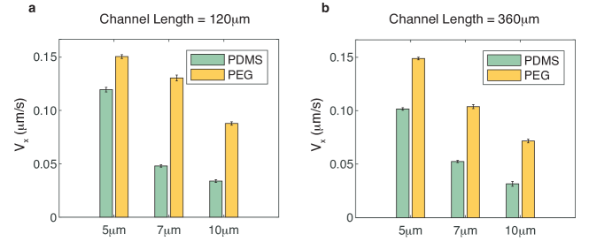
Figure S11: Average cell speed for different chamber heights and substrate composition for channel length $L=120\mu$m, corresponding to a gradient of 0.83 nM/$\mu$m, and $L=360\mu$m, corresponding to a gradient of 0.28 nM/$\mu$m.

References

- Munjal and Lecuit (2014) A. Munjal and T. Lecuit, Development 141, 1789 (2014).
- Kölsch et al. (2008) V. Kölsch, P. G. Charest, and R. A. Firtel, J Cell Sci 121, 551 (2008).
- Wirtz et al. (2011) D. Wirtz, K. Konstantopoulos, and P. C. Searson, Nature Reviews Cancer 11, 512 (2011).
- Geiger et al. (2009) B. Geiger, J. P. Spatz, and A. D. Bershadsky, Nature reviews Molecular cell biology 10, 21 (2009).
- Charras and Sahai (2014) G. Charras and E. Sahai, Nature reviews Molecular cell biology 15, 813 (2014).
- Chan and Odde (2008) C. E. Chan and D. J. Odde, Science 322, 1687 (2008).
- Harris et al. (1980) A. K. Harris, P. Wild, and D. Stopak, Science 208, 177 (1980).
- Frisch and Thoumine (2002) T. Frisch and O. Thoumine, Journal of biomechanics 35, 1137 (2002).
- Keren et al. (2008a) K. Keren, Z. Pincus, G. M. Allen, E. L. Barnhart, G. Marriott, A. Mogilner, and J. A. Theriot, Nature 453, 475 (2008a).
- Reinhart-King et al. (2005) C. A. Reinhart-King, M. Dembo, and D. A. Hammer, Biophysical journal 89, 676 (2005).
- Kockelkoren et al. (2003) J. Kockelkoren, H. Levine, and W.-J. Rappel, Physical Review E 68, 037702 (2003).
- Ziebert and Aranson (2013) F. Ziebert and I. S. Aranson, PloS one 8, e64511 (2013).
- Tjhung et al. (2015) E. Tjhung, A. Tiribocchi, D. Marenduzzo, and M. Cates, Nature communications 6, 5420 (2015).
- Zhao et al. (2010) Y. Zhao, S. Das, and Q. Du, Physical Review E 81, 041919 (2010).
- Mickel et al. (2011) W. Mickel, L. Joly, and T. Biben, The Journal of chemical physics 134, 094105 (2011).
- Carlsson (2011) A. Carlsson, New journal of physics 13, 073009 (2011).
- Stéphanou et al. (2008) A. Stéphanou, E. Mylona, M. Chaplain, and P. Tracqui, Journal of theoretical biology 253, 701 (2008).
- Mogilner (2009) A. Mogilner, Journal of mathematical biology 58, 105 (2009).
- Buenemann et al. (2010) M. Buenemann, H. Levine, W. J. Rappel, and L. M. Sander, Biophys J 99, 50 (2010).
- Alonso et al. (2018) S. Alonso, M. Stange, and C. Beta, PloS one 13, e0201977 (2018).
- Rubinstein et al. (2009) B. Rubinstein, M. F. Fournier, K. Jacobson, A. B. Verkhovsky, and A. Mogilner, Biophysical journal 97, 1853 (2009).
- Barnhart et al. (2011) E. L. Barnhart, K.-C. Lee, K. Keren, A. Mogilner, and J. A. Theriot, PLoS biology 9, e1001059 (2011).
- Bois et al. (2011a) J. S. Bois, F. Jülicher, and S. W. Grill, Physical review letters 106, 028103 (2011a).
- Shao et al. (2012) D. Shao, H. Levine, and W.-J. Rappel, Proc Natl Acad Sci U S A 109, 6851 (2012).
- Camley et al. (2013) B. A. Camley, Y. Zhao, B. Li, H. Levine, and W.-J. Rappel, Physical Review Letters 111, 158102 (2013).
- Goff et al. (2017) T. L. Goff, B. Liebchen, and D. Marenduzzo, arXiv preprint arXiv:1712.03138 (2017).
- Shao et al. (2010) D. Shao, W.-J. Rappel, and H. Levine, Physical Review Letters 105, 108104 (2010).
- Najem and Grant (2013) S. Najem and M. Grant, Physical Review E 88, 034702 (2013).
- Biben et al. (2005) T. Biben, K. Kassner, and C. Misbah, Physical Review E 72, 041921 (2005).
- Bois et al. (2011b) J. S. Bois, F. Jülicher, and S. W. Grill, Physical review letters 106, 028103 (2011b).
- Brakke (1992) K. A. Brakke, Experimental mathematics 1, 141 (1992).
- Kruse et al. (2006) K. Kruse, J. Joanny, F. Jülicher, and J. Prost, Physical biology 3, 130 (2006).
- Nagel et al. (2014) O. Nagel, C. Guven, M. Theves, M. Driscoll, W. Losert, and C. Beta, PloS one 9, e113382 (2014).
- Tanimoto and Sano (2014) H. Tanimoto and M. Sano, Biophysical journal 106, 16 (2014).
- Bausch et al. (1998) A. R. Bausch, F. Ziemann, A. A. Boulbitch, K. Jacobson, and E. Sackmann, Biophys. J. 75, 2038 (1998).
- Srinivasan and Walcott (2009) M. Srinivasan and S. Walcott, Physical Review E 80, 046124 (2009).
- Walcott and Sun (2010) S. Walcott and S. X. Sun, Proc Natl Acad Sci U S A 107, 7757 (2010).
- Huttenlocher et al. (1996) A. Huttenlocher, M. H. Ginsberg, and A. F. Horwitz, The Journal of cell biology 134, 1551 (1996).
- Palecek et al. (1997) S. P. Palecek, J. C. Loftus, M. H. Ginsberg, D. A. Lauffenburger, A. F. Horwitz, et al., Nature 385, 537 (1997).
- Gardel et al. (2008) M. L. Gardel, B. Sabass, L. Ji, G. Danuser, U. S. Schwarz, and C. M. Waterman, J cell Biol 183, 999 (2008).
- Loomis et al. (2012) W. F. Loomis, D. Fuller, E. Gutierrez, A. Groisman, and W.-J. Rappel, PloS one 7, e42033 (2012).
- Skoge et al. (2014) M. Skoge, H. Yue, M. Erickstad, A. Bae, H. Levine, A. Groisman, W. F. Loomis, and W.-J. Rappel, Proc Natl Acad Sci U S A 111, 14448 (2014).
- Tzvetkova-Chevolleau et al. (2009) T. Tzvetkova-Chevolleau, E. Yoxall, D. Fuard, F. Bruckert, P. Schiavone, and M. Weidenhaupt, Microelectronic Engineering 86, 1485 (2009).
- DiMilla et al. (1991) P. A. DiMilla, K. Barbee, and D. A. Lauffenburger, Biophys. J. 60, 15 (1991).
- Liu et al. (2015) Y.-J. Liu, M. Le Berre, F. Lautenschlaeger, P. Maiuri, A. Callan-Jones, M. Heuzé, T. Takaki, R. Voituriez, and M. Piel, Cell 160, 659 (2015).
- Camley et al. (2014) B. A. Camley, Y. Zhang, Y. Zhao, B. Li, E. Ben-Jacob, H. Levine, and W.-J. Rappel, Proc Natl Acad Sci U S A 111, 14770 (2014).
- Zhao et al. (2017) Y. Zhao, Y. Ma, H. Sun, B. Li, and Q. Du, arXiv preprint arXiv:1712.01951 (2017).
- Keren et al. (2008b) K. Keren, Z. Pincus, G. M. Allen, E. L. Barnhart, G. Marriott, A. Mogilner, and J. A. Theriot, Nature 453, 475 (2008b).
- Levine and Rappel (2013) H. Levine and W.-J. Rappel, Phys Today 66 (2013), 10.1063/PT.3.1884.
- Fuller et al. (2010) D. Fuller, W. Chen, M. Adler, A. Groisman, H. Levine, W.-J. Rappel, and W. F. Loomis, Proc Natl Acad Sci U S A 107, 9656 (2010).
- Sussman (1987) M. Sussman, in Methods in cell biology, Vol. 28 (Elsevier, 1987) pp. 9–29.
- Paliwal et al. (2007) S. Paliwal, P. A. Iglesias, K. Campbell, Z. Hilioti, A. Groisman, and A. Levchenko, Nature 446, 46 (2007).
- Skoge et al. (2010) M. Skoge, M. Adler, A. Groisman, H. Levine, W. F. Loomis, and W.-J. Rappel, Integrative Biology 2, 659 (2010).

References

- Camley et al. (2014) B. A. Camley, Y. Zhang, Y. Zhao, B. Li, E. Ben-Jacob, H. Levine, and W.-J. Rappel, Proc Natl Acad Sci U S A 111, 14770 (2014).
- Zhao et al. (2017) Y. Zhao, Y. Ma, H. Sun, B. Li, and Q. Du, arXiv preprint arXiv:1712.01951 (2017).
- Brakke (1992) K. A. Brakke, Experimental mathematics 1, 141 (1992).
- Shao et al. (2010) D. Shao, W.-J. Rappel, and H. Levine, Physical Review Letters 105, 108104 (2010).
- Camley et al. (2013) B. A. Camley, Y. Zhao, B. Li, H. Levine, and W.-J. Rappel, Physical Review Letters 111, 158102 (2013).
- Shao et al. (2012) D. Shao, H. Levine, and W.-J. Rappel, Proc Natl Acad Sci U S A 109, 6851 (2012).
- Carlsson (2011) A. Carlsson, New journal of physics 13, 073009 (2011).
- Keren et al. (2008) K. Keren, Z. Pincus, G. M. Allen, E. L. Barnhart, G. Marriott, A. Mogilner, and J. A. Theriot, Nature 453, 475 (2008).
- Levine and Rappel (2013) H. Levine and W.-J. Rappel, Phys Today 66 (2013), 10.1063/PT.3.1884.
- Fuller et al. (2010) D. Fuller, W. Chen, M. Adler, A. Groisman, H. Levine, W.-J. Rappel, and W. F. Loomis, Proc Natl Acad Sci U S A 107, 9656 (2010).
- Sussman (1987) M. Sussman, in Methods in cell biology, Vol. 28 (Elsevier, 1987) pp. 9–29.
- Paliwal et al. (2007) S. Paliwal, P. A. Iglesias, K. Campbell, Z. Hilioti, A. Groisman, and A. Levchenko, Nature 446, 46 (2007).
- Skoge et al. (2010) M. Skoge, M. Adler, A. Groisman, H. Levine, W. F. Loomis, and W.-J. Rappel, Integrative Biology 2, 659 (2010).
- Skoge et al. (2014) M. Skoge, H. Yue, M. Erickstad, A. Bae, H. Levine, A. Groisman, W. F. Loomis, and W.-J. Rappel, Proc Natl Acad Sci U S A 111, 14448 (2014).