Differential drag control scheme
for large constellation of Planet satellites
and on-orbit results

Abstract

A methodology is presented for the differential drag control of a large fleet of propulsion-less satellites deployed in the same orbit. The controller places satellites into a constellation with specified angular offsets and zero-relative speed. Time optimal phasing is achieved by first determining an appropriate relative placement, i.e. the order of the satellites. A second optimization problem is then solved as a large coupled system to find the drag command profile required for each satellite. The control authority is the available ratio of low-drag to high-drag ballistic coefficients of the satellites when operating in their background mode. The controller is able to successfully phase constellations with up to 100 satellites in simulations. On-orbit performance of the controller is demonstrated by phasing the Planet Flock 2p constellation of twelve cubesats launched in June 2016 into a 510 km sun-synchronous orbit.

1 Introduction

Due to easier access to space in recent years, there have been an increasing number of satellites launched. In addition to more launches, multiple satellites are deployed into orbit in one launch. The resent launch by the Indian Space Research Organisation (ISRO), for example, carried 104 satellites into orbit in February 2017. Other launches with a large number of satellites were a Russian Dnepr launch with 37 satellites, and an Orbital Antares rocket with 34 satellites onboard in 2004. Such launches are optimal for large constellations of small satellites that are in the same orbit but spread out in mean anomaly. The customized or randomized deployment velocities provided by the launcher can help in the spreading of the satellites. It is, unfortunately, not possible to first spread the satellites and then maintain relative phasing by only using the deployment velocities. To realize a fully spread and operationally useful constellation as shown in Figure 1, some propulsive capability is required.

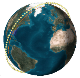
Figure 1: A line scanner configuration of satellites uniformly spread over the orbit

A constellation launched together typically consists of small homogeneous satellites. Adding propulsion to these satellites is an undertaking in terms of engineering, cost, and regulations. It might not be possible to fit the required propulsion subsystem for the desired $\Delta v$ due to size and weight constrains. Atmospheric drag, however, can be used to provide the relative velocities required to phase the constellation without additional mass if the altitude is sufficiently low. Differential drag changes the drag characteristics of space objects in order to control relative accelerations. The effective surface area perpendicular to the velocity vector acts as the actuator by changing the Ballistic Coefficient (BC).

Differential drag was first proposed for station keeping of a pair of satellites in 1989 ¹ by using drag plates. The control freedom is the angle of attack of the drag plates at $0^{\circ}$ or $90^{\circ}$ and the control law is based on the linearized Clohessy-Wiltshire equations of motion ². A similar strategy using a drag plate and including $J_{2}$ perturbation for satellite rendezvous is demonstrated by Bevilacqua ³ using the Schweighart-Sedwick linearized equations of motion ⁴. Rendezvous using a combination of differential drag for the first phase and low-thrust propulsion for the second precise phase is shown ⁵. Differential drag has also been combined with other perturbations such as Solar Radiation Pressure (SRP) for formation maneuvers ⁶.

Various types of controllers have been used to create trajectories such as an optimal control approach ⁷, Lyapunov based controllers ⁸, and sliding mode control ⁹. The extension of the two satellite problem into a multiple satellite problem has been carried out previously ¹⁰, ¹¹, ¹².

Differential drag has also been used for collision avoidance ¹³, ¹⁴. For satellites using differential drag, uncertainties in the atmosphere models have a noticeable effect on the uncertainty propagation of the satellites ¹⁵, ¹⁶. Another possible application of differential drag is to minimize the post-deployment probability of collision of nanosatellties ¹⁷.

To date, the Aerospace Corporation has demonstrated the use of differential drag on-orbit with small satellites, most recently with the AeroCube-4 mission in 2013 ¹⁸. This three-satellite mission was deployed into a 480 x 780 km orbit and operators were able to control along-track spacing of the satellites by selectively retracting solar panel wings. Orbcomm, with its constellation of 35 satellites in a 720 km altitude circular orbit, has also used differential drag to save propellant on its thrust-based station-keeping system ¹⁹.

The work presented in this paper shows an end to end implementation of a differential drag controller that phases out and performs station keeping on a constellation of satellites. The proposed controller converts the phasing problem into two separate optimization problems. The phase called Reslotting is only relevant when the constellation has more than two spacecraft where the relative phasing of the satellites is determined. The atmospheric density is allowed to be time varying, as is the case for real missions. Almost all prior work in differential drag, except for Guglielmo et al. ²⁰, assumes a constant density. Intra-constellation coupling is also included when computing the control. Coupling is considered by Harris and Açikmeşe ¹⁰ for up to five spacecraft with constant atmospheric drag. It is, however, unclear how this method scales up to 100 satellites. Li and Mason ²¹ treated a degenerate case of the multi-spacecraft problem limited to five satellites where the reference satellite performs no high drag maneuver. In addition to simulation results, on-orbit results of the successful phasing of 12 cubesats and the ongoing phasing of 88 cubesats is shown.

2 Differential-Drag Controller

As illustrated in Figure 2, the controller consists of three components. It first uses Cartesian position-velocity state vectors generated by orbit determination to estimate the relative motion of the satellites in the along-track direction. Two optimization problems aiming to minimize the total phasing time are then solved sequentially:

1. Slot Allocator: allocating each satellite to specific slots

2. Command Generator: finding appropriate high-drag windows required to reach the slots

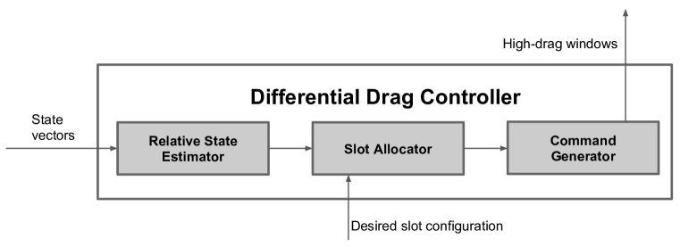
Figure 2: Controller produces high-drag windows from state vectors

2.1 Relative State Estimator

Since differential drag only controls the along-track dynamics of the satellite, the independent set of cartesian state vectors are reduced to relative Earth-centered angles shown in Figure 3 and their time derivatives.

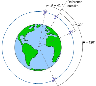
Figure 3: Relative state $\theta$ reduces complexity of control problem to along-track space

2.1.1 Initial Condition

Relative angles $\theta$ are calculated between each satellite and a reference satellite. This reference can be chosen to be any of the satellites but by convention the one that starts in the lowest orbit is used.

$\theta_{osc}$ is defined as the osculating Earth-centered relative angle between each satellite $i$ and the reference’s position vectors $R$, defined over $[0..2\pi)$ in the along-track direction (Equation 1). The half-plane ambiguity is solved with the reference pole vector $\vec{N}=||\vec{R}_{ref}\times\vec{V}_{ref}||$. It is noted that the reference satellite’s $\theta$ and $\dot{\theta}$ are always 0 by definition.

$$\theta_{osc,i}=angle_{[0..2\pi)}(\vec{R}_{ref},\vec{R}_{i})$$ (1)

The initial state consisting of $\theta$ and its time derivative, the angular velocity $\dot{\theta}$, are calculated as mean elements by fitting a line through the time history of $\theta_{osc}$ via least-squares as shown in Figure 4a. A 1-day fit period proves to be sufficient for capturing the motion of a typical LEO SSO orbit (400-600 km). To produce this time history, orbits are propagated under a 10x10 gravity and NRL-MSIS00 atmosphere force model.

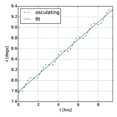
(a) Relative state $\theta_{0}$ and $\dot{\theta_{0}}$ from osculating motion

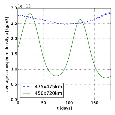
(b) Mean atmosphere density encountered by satellite, and hence control authority for differential drag, can fluctuate with time

Figure 4: Relative motion is estimated from propagated satellite state vectors

2.1.2 Control authority

To model the dynamics of satellites in high-drag, $\ddot{\theta}$ is also calculated, the relative angular acceleration of one satellite in high-drag mode relative to the reference satellite in low-drag. $\ddot{\theta}$ is a measure of available control authority, and is calculated across the simulation time horizon to effectively model the time-varying nature of control authority due to osculating motion of perigee and apogee and forecasted solar flux variations. This time-varying nature is important to capture when planning months ahead, and especially so for elliptical orbits where perigee and apogee vary cyclically over month timescales due the Earth’s gravity field (Figure 4b).

The mean dynamic pressure encountered by the reference satellite $q_{\text{ref}}$ throughout a discretized time period $\Delta t$ at time $k$ is first obtained using the atmosphere model with the latest space weather data.

$$q_{\text{ref},k}=\frac{1}{2}\overline{\rho v^{2}}$$ (2)

Next, the $\Delta V$ during the discretized time period is calculated using the observed ballistic coefficients $BC=\frac{m}{C_{d}A}$ in low and high-drag modes, $BC_{L}$ and $BC_{H}$ respectively:

$$\Delta V=q_{\text{ref},k}\Big{(}\frac{1}{BC_{L}}-\frac{1}{BC_{H}}\Big{)}\Delta t$$ (3)

The mean relative velocity $\dot{y}$ between the satellites is then evaluated, using the secular along-track component of the solution to Hill’s equations for relative motion ²²:

$$\dot{y}\approx-3\dot{y}_{0}=-3\Delta V=3q_{\text{ref},k}\Big{(}\frac{1}{BC_{H}}-\frac{1}{BC_{L}}\Big{)}\Delta t$$ (4)

Finally, the angular acceleration $\ddot{\theta}_{k}$ is evaluated during this discretized period, converting to angular coordinates using the reference satellite’s mean semi-major axis at epoch $\overline{a}_{\text{ref}}$:

$$\ddot{\theta}_{k}=\frac{\dot{y}\Delta t}{\overline{a}_{\text{ref}}}=\frac{3q_{\text{ref},k}}{\overline{a}_{\text{ref}}}\Big{(}\frac{1}{BC_{H}}-\frac{1}{BC_{L}}\Big{)}$$ (5)

2.1.3 Dynamics

The along-track dynamics of a constellation of $n$ satellites subject to time-discretized binary control inputs (low-drag or high-drag) can now be summarized by $n-1$ systems of Equation 6 for each satellite-reference pair. Note these systems are coupled since they all share the reference’s commands $u_{ref}$.

$$\begin{bmatrix}\theta\\ \dot{\theta}\end{bmatrix}_{k+1}=\begin{bmatrix}1&\Delta t\\ 0&1\end{bmatrix}\begin{bmatrix}\theta\\ \dot{\theta}\end{bmatrix}_{k}+\begin{bmatrix}0\\ B_{k}(u_{k})\end{bmatrix}$$ (6a)

where the control inputs $B_{k}$ are evaluated over the discretization period $\Delta t$ with the combined angular acceleration from the two satellites:

$$B_{k}(u_{k})=(-\ddot{\theta}_{ref,k}u_{ref,k}+\ddot{\theta}_{sat,k}u_{sat,k})\Delta t$$ (6b)

and high-drag commands $u_{i,k}$ are defined by:

$$u_{i,k}=\begin{cases}0\quad\text{if {i} is in low-drag at}\quad t_{k}\\ 1\quad\text{if {i} is in high-drag at}\quad t_{k}\end{cases}$$ (6c)

2.2 Slot Allocator

With the control problem reduced to optimization in relative-motion $\theta$ space, satellite ordering relative to one another is first determined to minimize predicted phasing time. The Dove satellites are interchangeable, so optimization is targeted to seek the lowest phasing time that achieves the desired slot vector irrespective of satellite order. As shown in Figure 5, the judicious assignment of satellites to slots is important for minimizing the time to phase of the constellation. Figure 5a shows a phasing attempt when target slots are assigned randomly, while Figure 5b starts with the same initial condition but slots have been allocated optimally to minimize time to phase.

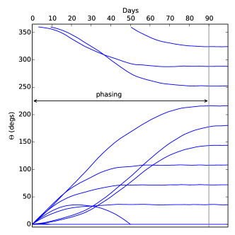
(a) random slot order: $\Delta t_{\text{phase}}=90$ days

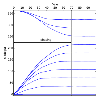
(b) optimal slot order: $\Delta t_{\text{phase}}=70$ days

Figure 5: Allocating slots judiciously significantly lowers the time required to phase a constellation.

2.2.1 Slots

A vector of slots is defined, where a slot is a desired $\theta_{f}$ for the final state of slot with $\dot{\theta}_{f}=0$. Various examples of slot configurations are shown in Figure 6. Equally-spaced satellites make sense for minimizing imaging swath overlap and ground station conflicts, while the fixed-spaced configuration is ideal for realizing a line scanner with adjacent swaths.

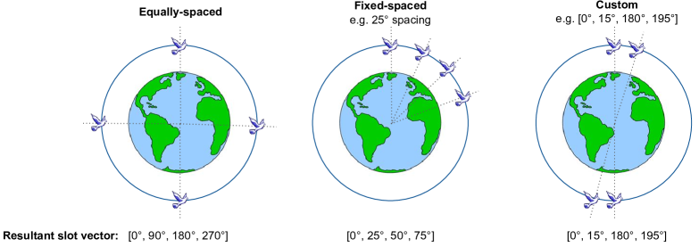
Figure 6: Slot vector describes desired relative placement of satellites

2.2.2 Flip-flop solution

Since the objective is to minimize phasing time, there is a need to estimate the amount of time required to achieve a certain slot configuration $\begin{bmatrix}\theta&\dot{\theta}\end{bmatrix}^{T}_{f}$ given the initial condition $\begin{bmatrix}\theta&\dot{\theta}\end{bmatrix}^{T}_{0}$ of each non-reference satellite. A method is introduced for solving the phasing time of a two-satellite constellation open-loop; to be used subsequently in the slot allocation optimizer.

The time-optimal solution for phasing two-satellites always has two phases (Figure 7): one satellite high-drags for a duration $\Delta t_{A}$ while the other low-drags (flip), then the roles reverse for another duration $\Delta t_{B}$ (flop). The solution to this control problem (duration of each phase, which satellite starts first) can be found analytically if assuming time-invariant $\ddot{\theta}$ (see Appendix B). The general problem can also be solved numerically via a line search as outlined in Algorithm 1, where the relative motion is propagated with the discretized equations of motion from Equation 6 to account for time-varying $\ddot{\theta}$.

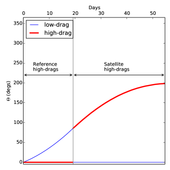
Figure 7: Flip-flop solution provides the time-optimal schedule for phasing two satellites

Algorithm 1 Flip-flop solution

1:procedure Solve two-satellite flip-flop problem

2:     try both order combinations for first sat to high-drag (one has a bracketed root in line search)

3:     while line searching to find $\Delta t_{A}$ such that $\theta_{f}=\theta_{f,desired}$ do

4:         prop via Eq 6 first sat in high-drag for $\Delta t_{A}$ then second in high-drag until $\dot{\theta}_{f}=\dot{\theta}_{f,desired}$

5:     end while

6:     output $\Delta t_{\text{phase}}=\Delta t_{A}+\Delta t_{B}$, and order in which satellites high-drag.

7:end procedure

2.2.3 Optimizer

The optimal slot configuration is solved for by selecting the order which minimizes the largest $\Delta t_{\text{phase}}$ of each reference-satellite pair. Algorithm 2 describes an implementation using simulated annealing ²³ wherein random perturbations are made to the slot configuration and kept if it satisfies an acceptance probability described in equation 7. It is found that values of $k_{max}=10^{6}$ and $t_{0}=100$ produce good results for typical differential drag scenarios.

Algorithm 2 Slot Allocator

1:procedure Obtain slot configuration for minimum time phasing

2:     for $k$ through $k_{max}$ do

3:         create $\text{slot}_{new}$ from slot by randomly swapping two satellites

4:         compute $\Delta t$ to phase for all reference-sat pairs with Algorithm 1

5:         if $P(\Delta t_{\text{max,old}},\Delta t_{\text{max,new}},k,k_{max})\geq\text{random}(0,1)$ then

6:              slot $\leftarrow\text{slot}_{new}$

7:         end if

8:     end for

9:end procedure

$$P(\text{cost},\text{cost}_{\text{new}},k,k_{max})=\begin{cases}1\quad\text{if cost}_{\text{new}}<\text{cost}\\ \exp{(\frac{\text{cost}-\text{cost}_{\text{new}}}{t})}\quad\text{if cost}_{\text{new}}\geq\text{cost with}\quad t=t_{0}(1-\frac{k}{k_{max}})\end{cases}$$ (7)

If the condition $\Delta t_{\text{max,old}}=\Delta t_{\text{max,new}}$ is reached, because the reference-satellite pair with the maximum phasing time is the same in the nominal and perturbed slot configurations, one then backs up to comparing the second greatest $\Delta t_{\text{phase}}$ (or next greatest if still equal).

When computing $\Delta t$ to phase to a particular slot, one also solves for which $2\pi$ offset to use by trying several neighboring $2\pi$ multiples and selecting the one with lowest phasing time.

2.3 Command Generator

Now that a final desired state $\theta_{f}$ is determined for each satellite, a set of high-drag commands is needed to guide the satellites to their desired slots in minimum time (Figure 8).

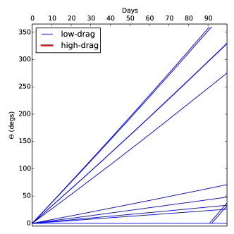
(a) without commands

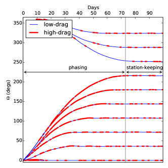
(b) with commands

Figure 8: Time-discretized high-drag commands are assigned to achieve desired slots

High-drag commands are discretized for simulation with Equation 6 across a time horizon that sufficiently captures the required settling time as estimated by the flip-flop solutions. The initial guess for the command matrix $u$ comes from the superposition of commands from flip-flop solutions to each reference-satellite sub-problem, or alternatively from the commands of the last time the controller was run. $u$ is then perturbed to converge satellites to their assigned slots via simulated annealing per the procedure described in Algorithm 3.

Algorithm 3 Command generator

1:procedure Obtain high-drag commands to target slots in minimum time

2:     for $k$ through $k_{max}$ do

3:         create $u_{new}$ with randomly flipped command $u_{sat=i,t=k}$

4:         compute finals states $\theta_{i,f}$ under $u_{new}$ with eq. 6

5:         compute $\text{cost}_{new}=\sum_{i}(\theta_{i,f}-\theta_{i,desired})^{2}$

6:         if $P(\text{cost}_{old},\text{cost}_{new},k,k_{max})\geq\text{random}(0,1)$ then

7:              $u\leftarrow u_{new}$

8:         end if

9:     end for

10:end procedure

During the station-keeping phase, the default high-drag mode is replaced with one that performs high-drag only a fraction of the time (e.g. 25%) to minimize the lifetime lost to drag since full control authority is no longer required. This also has the desireable side effect of shortening the limit cycle (station-keeping phasing error) when the time discretization period is kept constant.

3 Results

Results from the simulation and on-orbit implementation of the controller presented in Section 2 are presented here. All simulations and results use Planet’s Dove satellites. The various attitude modes of Planet’s Dove satellites exhibit a large difference in cross-sectional area thanks to their deployed solar panels, as shown in Figure 9.

(a) Orthographic projections with cross-sectional areas.

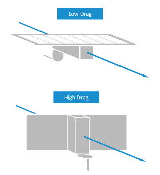
(b) High-drag and low-drag attitudes

Figure 9: Attitude modes of Dove satellite enable large drag area ratios

Although there is a 10:1 ratio between solar-panel and telescope facing cross-sectional areas, only a 3:1 ratio in orbit-derived ballistic coefficients (BC) is observed in reality. This reduction in control authority is due to several factors:

• Satellite duty-cycle: a satellite only executes the desired low-drag or high-drag mode when it is neither imaging nor downlinking. In imaging mode, the satellite presents a cross-sectional area between low and high-drag areas, while during downlinks the satellite tracks the ground station with its antenna boresight (co-aligned with telescope).

• Attitude pointing accuracy: attitude errors effectively reduce the ratio of high to low-drag cross-section areas. For example when not imaging or downlinking, the satellites are not using the star camera for attitude determination, resulting in deviations from modeled area.

• Skin friction effects: even in a perfect low-drag attitude, the large solar panel faces parallel to the velocity vector still contribute to drag via skin friction effects ²⁴, resulting in the low-drag mode having a higher drag coefficient $c_{d}$.

3.1 Performance of Controller

The main contributions of the proposed controller is the slot allocator and solving for the trajectories of all satellites as one highly coupled system. The coupling occurs due to the various flip-flop solutions possible requiring conflicting high-drag windows for the reference satellite.

Although the current controller reliably produces a robust solution, there are a few possible for improvements: a one-step optimizer and second-order optimizations. A source of future work is to solve the two optimization steps in one, by both assigning slots and generating commands in a single optimization loop. This would account for inter satellite-pair coupling effects, but it is currently computationally prohibitive to nest the command generator in the slot allocator. Finally, it would be of interest to implement second-order objective functions such as minimizing clustering during early stages of phasing, and minimizing station-keeping control effort given a specified control box.

3.2 In-Space Results

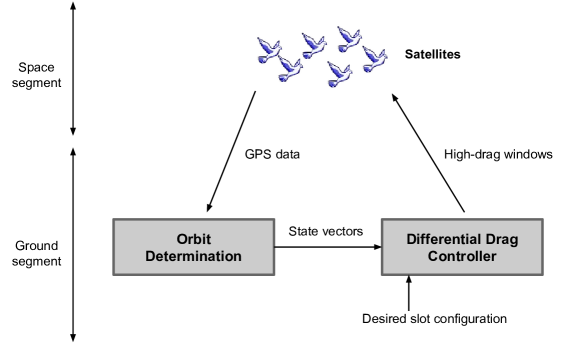
Figure 10: Orbit determination and differential drag controller runs on the ground

For satellite operations, all estimation and control for differential drag is performed on the ground (Figure 10). GPS data is regularly downloaded during X-band passes and ground-based orbit determination maintains state vector ephemerides for each satellite. The differential drag controller then uses these state vectors and the desired slot configuration to produce a set of high-drag commands that are uploaded to the satellite. For Planet’s operational orbits in the neighborhood of 500 km altitude, it is found that a controller update and time discretization of 1-day are sufficient for achieving desired performance.

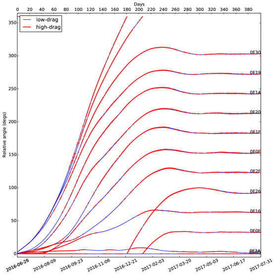
Figure 11: On-orbit results from Flock 2p

The differential drag controller described in this paper was applied to Flock 2p, a set of 12 satellites launched into a circular 510 km sun-synchronous orbit in June 2016. The satellites were deployed with a non-uniform total spread of 0.5 m/s along-track $\Delta V$ (deployer ejection speed is 1 m/s, along-track spread results from upper stage attitude schedule), and the controller allocated high-drag commands that initially increased this spread before converging to the desired slot configuration. The orbit-derived relative motion and commanded high-drag windows are shown in Figure 11. The same information is presented in a polar plot in Figure 14 of Appendix A. This relative motion plot can be recreated using JSpOC TLEs (CATIDs 41606, 41608-41618) or publicly-available Planet-produced ephemerides. The plan for Flock 2p was to achieve an equally-spaced constellation to minimize swath overlap and antenna conflicts, except for a pair of satellites that would maintain $3.6^{\circ}$ spacing to demonstrate the line scanner imaging strategy.

The primary lesson learned from automated on-orbit control of Flock 2p is to account for the significant unmodeled variations in effective BC. These fluctuations have been treated extensively by others ²⁵, and its specifics as encountered by Planet’s differential drag phasing are discussed below. Figure 12a shows the expected versus actual BCs; the expected values were pre-launch estimates based on an older Flock launched into a 600 km orbit in 2014. Figure 12b shows the resulting available control authority with pre-launch BCs using the solar flux prediction data at the time, and the actual control authority available from post-processed orbit data. One can see that the actual control authority available was significantly less than that predicted, by up to 50% 6 months after launch. This underestimation of control authority is responsible for the overshoot observed in Figure 11; and caused some churn with the slot allocator as it attempted to continuously target slots using its optimistic estimate of control authority.

Even though the satellites’ attitude control systems were consistent at maintaining low and high-drag modes, the resulting BCs exhibit large periodic fluctuations. The same fluctuating behavior has also been observed across year-long time-scales on satellites that are tumbling at rates much shorter than orbit fit-spans (therefore effectively presenting a constant cross-sectional area). One would expect the BCs in various consistent modes to be time-invariant when using a-posteriori solar flux data and industry standard atmosphere models like MSIS00 or Jacchia-Bowman 2008 ²⁶, so the fluctuating behavior of orbit-derived BCs is attributed to unmodeled atmospheric density variations due to solar phenomena (the period of the fluctuations also matches the Sun’s synodic period of 26 days). Atmosphere models have evolved in complexity, but they still fundamentally rely on a handful or less of channels of solar data. Since the Sun is the greatest contributor to these atmospheric density fluctuations, there must be potential for improved atmosphere models that make use of more data from the Sun, perhaps 10’s or 100’s channels and at higher frequencies from various measurement platforms that were not historically available.

The mitigation was to continuously update the controller’s estimate of low and high-drag BCs based on observed control authority from satellites in those modes.

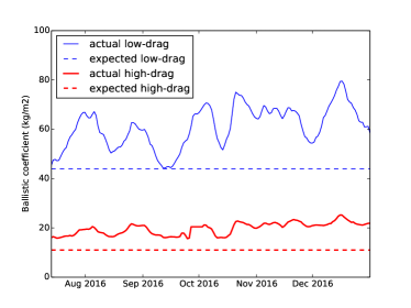
(a) Ballistic Coefficients (BC)

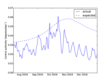
(b) Control authority

Figure 12: Expected vs. actual atmosphere-dependend performance

3.3 Future Contellations

Planet recently launched Flock 3p on February 14th 2017 into a 505 km altitude orbit. It consists of 88 Doves that were individually deployed and targeted to achieve a roughly uniform distribution of along-track $\Delta V$’s. The total initial spread is 2 m/s, spanning two groups of satellites, with a gap in the middle consisting of 13 non-Planet satellites. Figure 13 shows the simulated behavior of Flock 3p from deployment through station-keeping. The same information is presented in a polar plot in Figure 15 of Appendix A. The simulation factors in the fact that not all satellites are eligible to perform differential drag maneuvers right-away, as commissioning of specific satellites are staggered over the first 80 days.

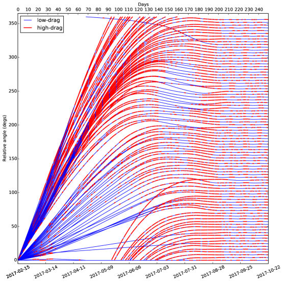
Figure 13: Simulation of Flock 3p phasing and station-keeping

4 Conclusion

This paper details a controller design for phasing and station-keeping large fleets of satellites with only differential drag. The controller works in three steps: relative motion estimation, slot allocating and high-drag command generation for the entire couple system.

Relative motion is first estimated in the along-track direction to obtain the mean angular separation angle and speed between each satellite and a designated reference. The satellites are assumed to be commandable into discrete low and high-drag modes, and angular acceleration for each mode is evaluated across a time horizon of interest to capture variations in mean atmospheric density.

Two optimization problems are then solved sequentially: the first to assign each satellite to a specific constellation slot and the second to generate time-discretized commands to guide each satellite to its slot using a coupled system. Both optimization problems seek to minimize the required phasing time given the available control authority, and are solved with simulated annealing, a method that lends well to the discretized nature of the problem. They also make use of the solution to the two-satellite sub-problem to either estimate the required phasing time or provide an initial guess to the general multi-satellite problem. Although both components are required for an optimal solution, the coupling of the system has a larger influence on the optimality and feasibility of the solutions.

The closed-loop performance of the controller is demonstrated with an operational fleet of twelve satellites, and it is also being applied to another fleet of 88 satellites that was recently launched in February 2017.

5 Acknowledgments

The authors would like to acknowledge Planet’s Missions and Spacecraft Design teams for putting together all the pieces needed to execute the automated differential drag operations described in the paper.

Appendix

.1 Polar Plots

Figures 14 and 15 are polar projections of Figures 11 and 13 respectively. Radial axis shows time (in days), while relative angle is on the $\theta$ axis. These polar projections better illustrate the relative angles that wrap around, at the cost of a time axis that is harder to read.

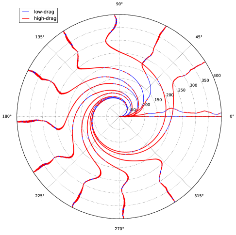
Figure 14: On-orbit results from Flock 2p

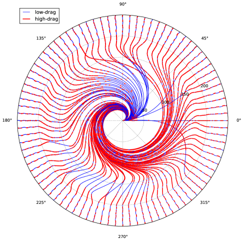
Figure 15: Simulation of Flock 3p phasing and station-keeping

.2 Analytic solution for two satellite case

This section presents the analytical solution to the time-optimal open-loop differential drag control of two satellites under time-invariant control authority $\ddot{\theta}$. The initial relative motion is given by $\begin{bmatrix}\theta&\dot{\theta}\end{bmatrix}^{T}_{0}$ and the final condition by $\begin{bmatrix}\theta&\dot{\theta}\end{bmatrix}^{T}_{f}$.

The solution consists of two phases (Figure 7): one satellite high-drags for a duration $\Delta t_{A}$ while the other low-drags, then the roles reverse for another duration $\Delta t_{B}$. If the reference high-drags first, the effective control authority during phases A and B are $\ddot{\theta}_{A}=-\ddot{\theta}$ and $\ddot{\theta}_{B}=\ddot{\theta}$ respectively. Similarly if the satellite high-drags first, then one has $\ddot{\theta}_{A}=\ddot{\theta}$ and $\ddot{\theta}_{B}=-\ddot{\theta}$ respectively.

The relative motion at the mid-point between phases A and B is expressed as $\begin{bmatrix}\theta&\dot{\theta}\end{bmatrix}^{T}_{m}$:

$$\begin{split}\theta_{m}&=\theta_{0}+\dot{\theta}_{0}\Delta t_{A}+\frac{1}{2}\ddot{\theta}_{A}\Delta t_{A}^{2}\\ \dot{\theta}_{m}&=\dot{\theta}_{0}+\ddot{\theta}_{A}\Delta t_{A}\end{split}$$ (8)

The final condition after phase B is then expressed as:

$$\begin{split}\theta_{f}&=\theta_{m}+\dot{\theta}_{m}\Delta t_{B}+\frac{1}{2}\ddot{\theta}_{B}\Delta t_{B}^{2}\\ \dot{\theta}_{f}&=\dot{\theta}_{m}+\ddot{\theta}_{B}\Delta t_{B}\end{split}$$ (9)

$\Delta t_{A}$ and $\Delta t_{B}$ are solved for from equations 8 and 9 by first eliminating $\theta_{m}$ and $\dot{\theta}_{m}$, and introducing the short hands $\Delta\theta=\theta_{f}-\theta_{0}$ and $\Delta\dot{\theta}=\dot{\theta}_{f}-\dot{\theta}_{0}$, to reveal $\Delta t_{B}$ as a function of $\Delta t_{A}$:

$$\Delta t_{B}=\frac{\Delta\dot{\theta}-\ddot{\theta}_{A}\Delta t_{A}}{\ddot{\theta}_{B}}$$ (10)

and $\Delta t_{A}$ from the quadratic:

$$\Bigg{[}\frac{1}{2}\ddot{\theta}_{A}\bigg{(}\frac{\ddot{\theta}_{A}}{\ddot{\theta}_{B}}-1\bigg{)}\Bigg{]}\Delta t_{A}^{2}+\Bigg{[}\dot{\theta}_{0}\bigg{(}\frac{\ddot{\theta}_{A}}{\ddot{\theta}_{B}}-1\bigg{)}\Bigg{]}\Delta t_{A}+\Bigg{[}\Delta\theta-\frac{\Delta\dot{\theta}}{\ddot{\theta}_{B}}\bigg{(}\dot{\theta}_{0}+\frac{1}{2}\Delta\dot{\theta}\bigg{)}\Bigg{]}=0\\$$ (11)

There are four possible solutions to the ($\Delta t_{A}$, $\Delta t_{B}$) couple given the ambiguity of which satellite should high-drag first, and the two roots to Equation 11, but only one couple has positive real values, the physical solution to the problem.

References

- 1 C. Leonard, W. Hollister, and E. Bergmann, “Orbital Formationkeeping with Differential Drag,” AIAA Journal of Guidance, Control, and Dynamics, Vol. 12, No. 1, 1989, pp. 108–113, 10.2514/3.20374.
- 2 W. H. Clohessy and R. S. Wiltshire, “Terminal Guidance System for Satellite Rendezvous,” Journal of the Aerospace Sciences, Vol. 27, No. 9, 1960, pp. 653 – 658, 10.2514/8.8704.
- 3 R. Bevilacqua and M. Romano, “Rendezvous Maneuvers of Multiple Spacecraft Using Differential Drag Under J2 Perturbation,” Journal of Guidance, Control, and Dynamics, Vol. 31, No. 6, 2008, pp. 1595–1607, 10.2514/1.36362.
- 4 S. A. Schweighart and R. J. Sedwick, “High-Fidelity Linearized J Model for Satellite Formation Flight,” Journal of Guidance, Control, and Dynamics, Vol. 25, No. 6, 2002, pp. 1073–1080, 10.2514/2.4986.
- 5 R. Bevilacqua, J. S. Hall, and M. Romano, “Multiple spacecraft rendezvous maneuvers by differential drag and low thrust engines,” Celestial Mechanics and Dynamical Astronomy, Vol. 106, No. 1, 2009, p. 69, 10.1007/s10569-009-9240-3.
- 6 D. Spiller, F. Curti, and C. Circi, “Minimum-Time Reconfiguration Maneuvers of Satellite Formations Using Perturbation Forces,” Journal of Guidance, Control, and Dynamics, Ahead of print, 2017, 10.2514/1.G002382.
- 7 L. Dell’Elce and G. Kerschen, “Optimal propellantless rendez-vous using differential drag,” Acta Astronautica, Vol. 109, 2015, pp. 112 – 123, 10.1016/j.actaastro.2015.01.011.
- 8 D. Pérez and R. Bevilacqua, “Lyapunov-Based Adaptive Feedback for Spacecraft Planar Relative Maneuvering via Differential Drag,” Journal of Guidance, Control, and Dynamics, Vol. 37, No. 5, 2014, pp. 1678–1684, 10.2514/1.G000191.
- 9 S. Varma and K. D. Kumar, “Multiple Satellite Formation Flying Using Differential Aerodynamic Drag,” Journal of Spacecraft and Rockets, Vol. 49, No. 2, 2012, pp. 325–336, 10.2514/1.52395.
- 10 M. W. Harris and B. Açikmeşe, “Minimum time rendezvous of multiple spacecraft using differential drag,” Journal of Guidance, Control, and Dynamics, Vol. 37, 3 2014, pp. 365–373, 10.2514/1.61505.
- 11 B. S. Kumar, A. Ng, K. Yoshihara, and A. D. Ruiter, “Differential Drag as a Means of Spacecraft Formation Control,” 2007 IEEE Aerospace Conference, March 2007, pp. 1–9, 10.1109/AERO.2007.352790.
- 12 M. Horsley, “An investigation into using differential drag for controlling a formation of CubeSats,” Advanced Maui Optical and Space Surveillance Technologies Conference, Sept. 2011, p. E28.
- 13 D. Mishne and E. Edlerman, “Collision-Avoidance Maneuver of Satellites Using Drag and Solar Radiation Pressure,” Journal of Guidance, Control, and Dynamics, Ahead of print, 2017, 10.2514/1.G002376.
- 14 X. Huang, Y. Yan, and Y. Zhou, “Underactuated spacecraft formation reconfiguration with collision avoidance,” Acta Astronautica, Vol. 131, 2017, pp. 166 – 181, http://doi.org/10.1016/j.actaastro.2016.11.037.
- 15 L. Mazal, D. Pérez, R. Bevilacqua, and C. F., “Spacecraft Rendezvous by Differential Drag Under Uncertainties,” Journal of Guidance, Control, and Dynamics, Vol. 39, August 2016, pp. 1721–1733, 10.2514/1.G001785.
- 16 O. Ben-Yaacov, A. Ivantsov, and P. Gurfil, “Covariance analysis of differential drag-based satellite cluster flight,” Acta Astronautica, Vol. 123, 2016, pp. 387 – 396, 10.1016/j.actaastro.2015.12.035.
- 17 J. A. Atchison and A. Q. Rogers, “Operational Methodology for Large-Scale Deployment of Nanosatellites into Low Earth Orbit,” Journal of Spacecraft and Rockets, Vol. 53, No. 5, 2016, pp. 799–810, 10.2514/1.A33361.
- 18 J. Gangestad, B. Hardy, and D. Hinkley, “Operations, Orbit Determination, and Formation Control of the AeroCube-4 CubeSats,” 27th Annual AIAA/USU Conference on Small Satellites, No. SSC13-X-4, Logan, Utah, 2013.
- 19 T. D. Maclay and C. Tuttle, “Satellite stationkeeping of the ORBCOMM constellation via active control of atmospheric drag: operations, constraints, and performance,” AAS/AIAA Space Flight Mechaics Meeting, No. AAS 05-152, Copper Mountain, CO, January 2005.
- 20 D. Guglielmo, D. Pérez, R. Bevilacqua, and L. Mazal, “Spacecraft relative guidance via spatio-temporal resolution in atmospheric density forecasting,” Acta Astronautica, Vol. 129, 2016, pp. 32 – 43, 10.1016/j.actaastro.2016.08.016.
- 21 A. S. Li and J. Mason, “Optimal Utility of Satellite Constelllation Separation with Differential Drag,” AIAA/AAS Astrodynamics Specialist Conference, AIAA SPACE Forum, No. AIAA 2014-4112, San Diego, CA, August 2014, 10.2514/6.2014-4112.
- 22 D. Vallado, Fundamentals of Astrodynamics and Applications. Microcosm Press and Springer, 3 ed., 2007. page 387.
- 23 A. Khachaturyan, S. Semenovskaya, and B. Vainshtein, “Statistical-Thermodynamic Approach to Determination of Structure Amplitude Phases,” Soviet Physics, Crystallography, Vol. 24, No. 5, 1979, pp. 519–524.
- 24 G. Koppenwallner, “Satellite Aerodynamics and Determination of Thermospheric Density and Wind,” American Institute of Physics Conference Series, Vol. 1333 of American Institute of Physics Conference Series, May 2011, pp. 1307–1312, 10.1063/1.3562824.
- 25 D. A. Vallado and D. Finkleman, “A critical assessment of satellite drag and atmospheric density modeling,” Acta Astronautica, Vol. 95, 2014, pp. 141 – 165, http://doi.org/10.1016/j.actaastro.2013.10.005.
- 26 B. R. Bowman, W. K. Tobiska, F. Marcos, and C. Huang, “The Thermospheric Density Model JB2008 using New EUV Solar and Geomagnetic Indices,” 37th COSPAR Scientific Assembly, Vol. 37 of COSPAR Meeting, 2008, p. 367.