EUROPEAN ORGANIZATION FOR NUCLEAR RESEARCH (CERN)

​​​ CERN-EP-2018-135 LHCb-PAPER-2018-017 21 September 2018

Measurement of the CKM angle $\gamma$

using ${{B}^{\pm}}\rightarrow D{{K}^{\pm}}$ with

$D\rightarrow{{K}^{0}_{\mathrm{\scriptscriptstyle S}}}{{\pi}^{+}}{{\pi}^{-}},{{K}^{0}_{\mathrm{\scriptscriptstyle S}}}{{K}^{+}}{{K}^{-}}$ decays

LHCb collaboration

A binned Dalitz plot analysis of $B^{\pm}\rightarrow DK^{\pm}$ decays, with $D\rightarrow{{K}^{0}_{\mathrm{\scriptscriptstyle S}}}{{\pi}^{+}}{{\pi}^{-}}$ and $D\rightarrow{{K}^{0}_{\mathrm{\scriptscriptstyle S}}}{{K}^{+}}{{K}^{-}}$, is used to perform a measurement of the $C\!P$-violating observables $x_{\pm}$ and $y_{\pm}$, which are sensitive to the Cabibbo-Kobayashi-Maskawa angle $\gamma$. The analysis is performed without assuming any $D$ decay model, through the use of information on the strong-phase variation over the Dalitz plot from the CLEO collaboration. Using a sample of proton-proton collision data collected with the LHCb experiment in 2015 and 2016, and corresponding to an integrated luminosity of 2.0$\mbox{\,fb}^{-1}$, the values of the $C\!P$ violation parameters are found to be $x_{-}=(9.0\pm 1.7\pm 0.7\pm 0.4)\times 10^{-2}$, $y_{-}=(2.1\pm 2.2\pm 0.5\pm 1.1)\times 10^{-2}$, $x_{+}=(-7.7\pm 1.9\pm 0.7\pm 0.4)\times 10^{-2}$, and $y_{+}=(-1.0\pm 1.9\pm 0.4\pm 0.9)\times 10^{-2}$. The first uncertainty is statistical, the second is systematic, and the third is due to the uncertainty on the strong-phase measurements. These values are used to obtain $\gamma=\left(87\,^{+11}_{-12}\right)^{\circ}$, $r_{B}=0.086^{+0.013}_{-0.014}$, and $\delta_{B}=(101\pm 11)^{\circ}$, where $r_{B}$ is the ratio between the suppressed and favoured $B$-decay amplitudes and $\delta_{B}$ is the corresponding strong-interaction phase difference. This measurement is combined with the result obtained using 2011 and 2012 data collected with the LHCb experiment, to give $\gamma=\left(80\,^{+10}_{\,-9}\right)^{\circ}$, $r_{B}=0.080\pm 0.011$, and $\delta_{B}=(110\pm 10)^{\circ}$.

Published in JHEP (2018) 2018: 176.

© 2024 CERN for the benefit of the LHCb collaboration. CC-BY-4.0 licence.

 

1 Introduction

The Standard Model (SM) description of $C\!P$ violation [1, 2] can be tested by overconstraining the angles of the Unitarity Triangle. The Cabibbo-Kobayashi-Maskawa (CKM) angle $\gamma\equiv\mathrm{arg}(-V_{ud}^{\phantom{\ast}}V_{ub}^{\ast}/V_{cd}^{\phantom{\ast}}V_{cb}^{\ast})$ is experimentally accessible through the interference between $\bar{b}\rightarrow\bar{c}u\bar{s}$ and $\bar{b}\rightarrow\bar{u}c\bar{s}$ transitions. It is the only CKM angle easily accessible in tree-level processes and it can be measured with negligible uncertainty from theory [3]. Hence, in the absence of new physics effects at tree level, a precision measurement of $\gamma$ provides a SM benchmark that can be compared with other CKM-matrix observables more likely to be affected by physics beyond the SM. Such comparisons are currently limited by the uncertainty on direct measurements of $\gamma$, which is about $5^{\circ}$ [4] and is driven by the LHCb average.

The effects of interference between $\bar{b}\rightarrow\bar{c}u\bar{s}$ and $\bar{b}\rightarrow\bar{u}c\bar{s}$ transitions can be probed by studying $C\!P$-violating observables in ${{B}^{\pm}}\rightarrow D{{K}^{\pm}}$ decays, where $D$ represents a ${D}^{0}$ or a ${\kern 1.99997pt\overline{\kern-1.99997ptD}{}}{}^{0}$ meson reconstructed in a final state that is common to both  [5, 6, 7]. This decay mode has been studied at LHCb with a wide range of $D$-meson final states to measure observables with sensitivity to $\gamma$ [8, 9, 10, 11]. In addition to these studies, other $B$ decays have also been used with a variety of techniques to determine $\gamma$ [12, 13, 14, 15].

This paper presents a model-independent study of the decay mode ${{B}^{\pm}}\rightarrow D{{K}^{\pm}}$, using $D\rightarrow{{K}^{0}_{\mathrm{\scriptscriptstyle S}}}{{\pi}^{+}}{{\pi}^{-}}$ and $D\rightarrow{{K}^{0}_{\mathrm{\scriptscriptstyle S}}}{{K}^{+}}{{K}^{-}}$ decays (denoted $D\rightarrow{{K}^{0}_{\mathrm{\scriptscriptstyle S}}}h^{+}h^{-}$ decays). The analysis utilises $pp$ collision data accumulated with LHCb in 2015 and 2016 at a centre-of-mass energy of $\sqrt{s}=13$ $\mathrm{\,Te\kern-1.00006ptV}$ and corresponding to a total integrated luminosity of $2.0\mbox{\,fb}^{-1}$. The result is combined with the result obtained by LHCb with the same analysis technique, using data collected in 2011 and 2012 (Run 1) at centre-of-mass energies of $\sqrt{s}=7$ $\mathrm{\,Te\kern-1.00006ptV}$ and $\sqrt{s}=8$ $\mathrm{\,Te\kern-1.00006ptV}$ [9].

The sensitivity to $\gamma$ is obtained by comparing the distributions in the Dalitz plots of $D\rightarrow{{K}^{0}_{\mathrm{\scriptscriptstyle S}}}h^{+}h^{-}$ decays from reconstructed $B^{+}$ and $B^{-}$ mesons [6, 7]. For this comparison, the variation of the strong-phase difference between ${D}^{0}$ and ${\kern 1.99997pt\overline{\kern-1.99997ptD}{}}{}^{0}$ decay amplitudes within the Dalitz plot needs to be known. An attractive, model-independent, approach makes use of direct measurements of the strong-phase variation over bins of the Dalitz plot [6, 16, 17]. The strong phase can be directly accessed by exploiting the quantum correlation of ${{D}^{0}}{{\kern 1.99997pt\overline{\kern-1.99997ptD}{}}{}^{0}}$ pairs from $\psi(3770)$ decays. Such measurements have been performed by the CLEO collaboration [18] and have been used by the LHCb [9] and Belle [19] collaborations to measure $\gamma$ in ${{B}^{\pm}}\rightarrow D{{K}^{\pm}}$ decays, and have also been used to study ${{B}^{0}}\rightarrow D{{K}^{*0}}$ decays  [20, 21]. An alternative method relies on amplitude models of $D\rightarrow{{K}^{0}_{\mathrm{\scriptscriptstyle S}}}h^{+}h^{-}$ decays, determined from flavour-tagged $D\rightarrow{{K}^{0}_{\mathrm{\scriptscriptstyle S}}}h^{+}h^{-}$ decays, to predict the strong-phase variation over the Dalitz plot. This method has been used for a variety of $B$ decays [22, 23, 24, 25, 26, 27, 28].

The separation of data into binned regions of the Dalitz plot leads to a loss of statistical sensitivity in comparison to using an amplitude model [16, 17]. However, the advantage of using the direct strong-phase measurements resides in the model-independent nature of the systematic uncertainties. Where the direct strong-phase measurements are used, there is only a systematic uncertainty associated with the finite precision of such measurements. Conversely, systematic uncertainties associated with determining a phase from an amplitude model are difficult to evaluate, as common approaches to amplitude-model building break the optical theorem [29]. Therefore, the loss in statistical precision is compensated by reliability in the evaluation of the systematic uncertainty, which is increasingly important as the overall precision on the CKM angle $\gamma$ improves.

2 Overview of the analysis

The amplitude of the decay $B^{-}\rightarrow DK^{-}$, $D\rightarrow{{K}^{0}_{\mathrm{\scriptscriptstyle S}}}h^{+}h^{-}$ can be written as a sum of the favoured $B^{-}\rightarrow D^{0}K^{-}$ and suppressed $B^{-}\rightarrow{{\kern 1.99997pt\overline{\kern-1.99997ptD}{}}{}^{0}}K^{-}$ contributions as

$$A_{B}(m_{-}^{2},m_{+}^{2})\propto\,A_{D}(m_{-}^{2},m_{+}^{2})+r_{B}e^{i(\delta_{B}-\gamma)}A_{{\kern 1.39998pt\overline{\kern-1.39998ptD}{}}}(m_{-}^{2},m_{+}^{2}),$$ (1)

where $m_{-}^{2}$ and $m_{+}^{2}$ are the squared invariant masses of the ${{K}^{0}_{\mathrm{\scriptscriptstyle S}}}h^{-}$ and ${{K}^{0}_{\mathrm{\scriptscriptstyle S}}}h^{+}$ particle combinations, respectively, that define the position of the decay in the Dalitz plot, $A_{D}(m_{-}^{2},m_{+}^{2})$ is the ${{D}^{0}}\rightarrow{{K}^{0}_{\mathrm{\scriptscriptstyle S}}}h^{+}h^{-}$ decay amplitude, and $A_{{\kern 1.39998pt\overline{\kern-1.39998ptD}{}}}(m_{-}^{2},m_{+}^{2})$ the ${{\kern 1.99997pt\overline{\kern-1.99997ptD}{}}{}^{0}}\rightarrow{{K}^{0}_{\mathrm{\scriptscriptstyle S}}}h^{+}h^{-}$ decay amplitude. The parameter $r_{B}$ is the ratio of the magnitudes of the $B^{-}\rightarrow{{\kern 1.99997pt\overline{\kern-1.99997ptD}{}}{}^{0}}K^{-}$ and $B^{-}\rightarrow{{D}^{0}}K^{-}$ amplitudes, while $\delta_{B}$ is their strong-phase difference. The equivalent expression for the charge-conjugated decay $B^{+}\rightarrow DK^{+}$ is obtained by making the substitutions $\gamma\rightarrow-\gamma$ and $A_{D}(m_{-}^{2},m_{+}^{2})\leftrightarrow A_{{\kern 1.39998pt\overline{\kern-1.39998ptD}{}}}(m_{-}^{2},m_{+}^{2})$. Neglecting $C\!P$ violation in charm decays, the charge-conjugated amplitudes satisfy the relation $A_{{\kern 1.39998pt\overline{\kern-1.39998ptD}{}}}(m^{2}_{-},m^{2}_{+})=A_{D}(m^{2}_{+},m^{2}_{-})$.

The $D$-decay Dalitz plot is partitioned into $2\times N$ bins labelled from $i=-N$ to $i=+N$ (excluding zero), symmetric around $m^{2}_{-}=m^{2}_{+}$ such that if $(m^{2}_{-},m^{2}_{+})$ is in bin $i$ then $(m^{2}_{+},m^{2}_{-})$ is in bin $-i$. By convention, the positive values of $i$ correspond to bins for which $m_{-}^{2}>m_{+}^{2}$. The strong-phase difference between the ${D}^{0}$ and ${\kern 1.99997pt\overline{\kern-1.99997ptD}{}}{}^{0}$-decay amplitudes at a given point on the Dalitz plot is denoted as $\delta_{D}(m_{-}^{2},m_{+}^{2})$. The cosine of $\delta_{D}(m_{-}^{2},m_{+}^{2})$ weighted by the $D$-decay amplitude and averaged over bin $i$ is written as $c_{i}$ [6], and is given by

$$c_{i} \equiv\frac{\int_{i}dm^{2}_{-}\,dm^{2}_{+}\,|A_{D}(m^{2}_{-},m^{2}_{+})||A_{D}(m^{2}_{+},m^{2}_{-})|\cos[\delta_{D}(m^{2}_{-},m^{2}_{+})-\delta_{D}(m^{2}_{+},m^{2}_{-})]}{\sqrt{\int_{i}dm^{2}_{-}\,dm^{2}_{+}\,|A_{D}(m^{2}_{-},m^{2}_{+})|^{2}\int_{i}dm^{2}_{-}\,dm^{2}_{+}\,|A_{D}(m^{2}_{+},m^{2}_{-})|^{2}}}\,,$$ (2)

where the integrals are evaluated over the phase space of bin $i$. An analogous expression can be written for $s_{i}$, which is the sine of the strong-phase difference weighted by the decay amplitude and averaged over the bin phase space. The values of $c_{i}$ and $s_{i}$ have been directly measured by the CLEO collaboration, exploiting quantum-correlated ${{D}^{0}}{{\kern 1.99997pt\overline{\kern-1.99997ptD}{}}{}^{0}}$ pairs produced at the $\psi(3770)$ resonance [18].

The measurements of $c_{i}$ and $s_{i}$ are available in four different $2\times 8$ binning schemes for the $D\rightarrow{{K}^{0}_{\mathrm{\scriptscriptstyle S}}}{{\pi}^{+}}{{\pi}^{-}}$ decay. This analysis uses the ‘optimal binning’ scheme where the bins have been chosen to optimise the statistical sensitivity to $\gamma$, as described in Ref. [18]. The optimisation was performed assuming a strong-phase difference distribution as predicted by the BaBar model presented in Ref. [23]. For the ${{K}^{0}_{\mathrm{\scriptscriptstyle S}}}{{K}^{+}}{{K}^{-}}$ final state, three choices of binning schemes are available, containing $2\times 2$, $2\times 3$, and $2\times 4$ bins. The guiding model used to determine the bin boundaries is taken from the BaBar study described in Ref. [24]. The $2\times 2$ binning scheme is chosen, due to the low signal yields in the $D\rightarrow{{K}^{0}_{\mathrm{\scriptscriptstyle S}}}{{K}^{+}}{{K}^{-}}$ mode. The same choice of bins was used in the LHCb Run 1 analysis [9]. The measurements of $c_{i}$ and $s_{i}$ are not biased by the use of a specific amplitude model in defining the bin boundaries. The choice of the model only affects this analysis to the extent that a poor model description of the underlying decay would result in a reduced statistical sensitivity of the $\gamma$ measurement. The binning choices for the two decay modes are shown in Fig. 1.

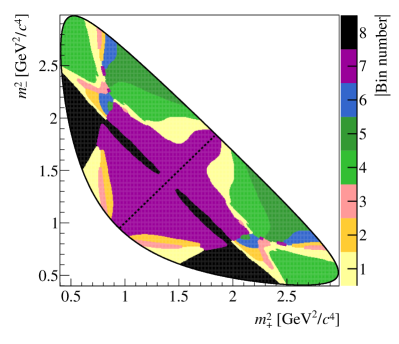
Figure 1: Binning schemes for (left) $D\rightarrow{{K}^{0}_{\mathrm{\scriptscriptstyle S}}}{{\pi}^{+}}{{\pi}^{-}}$ decays and (right) $D\rightarrow{{K}^{0}_{\mathrm{\scriptscriptstyle S}}}{{K}^{+}}{{K}^{-}}$ decays. The diagonal line separates the positive and negative bins, where the positive bins are in the region in which $m^{2}_{-}>m^{2}_{+}$ is satisfied.

The physics parameters of interest, $r_{B}$, $\delta_{B}$, and $\gamma$, are translated into four $C\!P$ obser-vables [22] that are measured in this analysis. These observables are defined as

$$x_{\pm}\equiv r_{B}\cos(\delta_{B}\pm\gamma){\rm\ \ and\ }\;y_{\pm}\equiv r_{B}\sin(\delta_{B}\pm\gamma).$$ (3)

It follows from Eq. (1) that the expected numbers of ${{B}^{+}}$ and ${{B}^{-}}$ decays in bin $i$, $N^{+}_{i}$ and $N^{-}_{i}$, are given by

$$\begin{split}N_{\pm i}^{+}&=h_{B^{+}}\left[F_{\mp i}+(x_{+}^{2}+y_{+}^{2})F_{\pm i}+2\sqrt{F_{i}F_{-i}}(x_{+}c_{\pm i}-y_{+}s_{\pm i})\right],\\ N_{\pm i}^{-}&=h_{B^{-}}\left[F_{\pm i}+(x_{-}^{2}+y_{-}^{2})F_{\mp i}+2\sqrt{F_{i}F_{-i}}(x_{-}c_{\pm i}+y_{-}s_{\pm i})\right],\end{split}$$ (4)

where $F_{i}$ are the fractions of decays in bin $i$ of the ${{D}^{0}}\rightarrow{{K}^{0}_{\mathrm{\scriptscriptstyle S}}}h^{+}h^{-}$ Dalitz plot, and $h_{B^{\pm}}$ are normalisation factors, which can be different for $B^{+}$ and $B^{-}$ due to production, detection, and $C\!P$ asymmetries. In this measurement, the integrated yields are not used to provide information on $x_{\pm}$ and $y_{\pm}$, and so the analysis is insensitive to such effects. From Eq. (4) it is seen that studying the distribution of candidates over the $D\rightarrow{{K}^{0}_{\mathrm{\scriptscriptstyle S}}}h^{+}h^{-}$ Dalitz plot gives access to the $x_{\pm}$ and $y_{\pm}$ observables. The detector and selection requirements placed on the data lead to a non-uniform efficiency over the Dalitz plot, which affects the $F_{i}$ parameters. The efficiency profile for the signal candidates is denoted as $\eta(m^{2}_{-},m^{2}_{+})$. The parameters $F_{i}$ can then be expressed as

$$F_{i}=\frac{\int_{i}dm^{2}_{-}dm^{2}_{+}|A_{D}(m^{2}_{-},m^{2}_{+})|^{2}\,\eta(m^{2}_{-},m^{2}_{+})}{\sum_{j}\int_{j}dm^{2}_{-}dm^{2}_{+}|A_{D}(m^{2}_{-},m^{2}_{+})|^{2}\,\eta(m^{2}_{-},m^{2}_{+})}\,.$$ (5)

The values of $F_{i}$ are determined from the control decay mode $\kern 1.79993pt\shortstack{{(\rule[2.15277pt]{12.50002pt}{0.51212pt})} \\ [-.7ex] $\kern-1.79993ptB$}{}\!\rightarrow{{D}^{*\pm}}\mu^{\mp}\shortstack{{(\rule[2.15277pt]{10.00002pt}{0.51212pt})} \\ [-.7ex] $\nu$}{}_{\!\!\mu}X$, where the ${D}^{*-}$ meson decays to ${\kern 1.99997pt\overline{\kern-1.99997ptD}{}}{}^{0}$ ${\pi}^{-}$ and the ${\kern 1.99997pt\overline{\kern-1.99997ptD}{}}{}^{0}$ meson decays to either the ${{K}^{0}_{\mathrm{\scriptscriptstyle S}}}{{\pi}^{+}}{{\pi}^{-}}$ or ${{K}^{0}_{\mathrm{\scriptscriptstyle S}}}{{K}^{+}}{{K}^{-}}$ final state. The symbol $X$ indicates other particles which may be produced in the decay but are not reconstructed. Samples of simulated events are used to correct for the small differences in efficiency arising through unavoidable differences in selecting $\kern 1.79993pt\shortstack{{(\rule[2.15277pt]{12.50002pt}{0.51212pt})} \\ [-.7ex] $\kern-1.79993ptB$}{}\!\rightarrow{{D}^{*\pm}}\mu^{\mp}\shortstack{{(\rule[2.15277pt]{10.00002pt}{0.51212pt})} \\ [-.7ex] $\nu$}{}_{\!\!\mu}X$ and ${{B}^{\pm}}\rightarrow D{{K}^{\pm}}$ decays, as discussed further in Sect. 5.

In addition to ${{B}^{\pm}}\rightarrow D{{K}^{\pm}}$ and $\kern 1.79993pt\shortstack{{(\rule[2.15277pt]{12.50002pt}{0.51212pt})} \\ [-.7ex] $\kern-1.79993ptB$}{}\!\rightarrow{{D}^{*\pm}}\mu^{\mp}\shortstack{{(\rule[2.15277pt]{10.00002pt}{0.51212pt})} \\ [-.7ex] $\nu$}{}_{\!\!\mu}X$ candidates, ${{B}^{\pm}}\rightarrow D{{\pi}^{\pm}}$ decays are selected. These provide an important control sample that is used to constrain the invariant-mass shape of the ${{B}^{\pm}}\rightarrow D{{K}^{\pm}}$ signal, as well as to determine the yield of ${{B}^{\pm}}\rightarrow D{{\pi}^{\pm}}$ decays misidentified as ${{B}^{\pm}}\rightarrow D{{K}^{\pm}}$ candidates. Note that this channel is not optimal for determining the values of $F_{i}$ as the small level of $C\!P$ violation in the decay leads to a significant systematic uncertainty, as was reported in Ref. [30]. This uncertainty is eliminated when using the flavour-specific semileptonic decay, in favour of a smaller systematic uncertainty associated with efficiency differences.

The effect of ${D}^{0}$–${\kern 1.99997pt\overline{\kern-1.99997ptD}{}}{}^{0}$ mixing was ignored in the above discussion. If the parameters $F_{i}$ are obtained from $\kern 1.79993pt\shortstack{{(\rule[2.15277pt]{12.50002pt}{0.51212pt})} \\ [-.7ex] $\kern-1.79993ptB$}{}\!\rightarrow{{D}^{*\pm}}\mu^{\mp}\shortstack{{(\rule[2.15277pt]{10.00002pt}{0.51212pt})} \\ [-.7ex] $\nu$}{}_{\!\!\mu}X$, where the ${D}^{*-}$ decays to ${\kern 1.99997pt\overline{\kern-1.99997ptD}{}}{}^{0}$ ${\pi}^{-}$, ${D}^{0}$–${\kern 1.99997pt\overline{\kern-1.99997ptD}{}}{}^{0}$ mixing has been shown to lead to a bias of approximately $0.2^{\circ}$ in the $\gamma$ determination [31], which is negligible for the current analysis. The effects of $C\!P$ violation in the neutral kaon system and of the different nuclear interaction cross-sections for ${K}^{0}$ and ${\kern 1.99997pt\overline{\kern-1.99997ptK}{}}{}^{0}$ mesons are discussed in Sect. 7, where a systematic uncertainty is assigned.

3 Detector and simulation

The LHCb detector [32, 33] is a single-arm forward spectrometer covering the pseudorapidity range $2<\eta<5$, designed for the study of particles containing $b$ or $c$ quarks. The detector includes a high-precision tracking system consisting of a silicon-strip vertex detector surrounding the $pp$ interaction region, a large-area silicon-strip detector located upstream of a dipole magnet with a bending power of about $4{\mathrm{\,Tm}}$, and three stations of silicon-strip detectors and straw drift tubes placed downstream of the magnet. The polarity of the dipole magnet is reversed periodically throughout data-taking. The tracking system provides a measurement of momentum, $p$, of charged particles with relative uncertainty that varies from 0.5% at low momentum to 1.0% at 200${\mathrm{\,Ge\kern-1.00006ptV\!/}c}$. The minimum distance of a track to a primary vertex (PV), the impact parameter (IP), is measured with a resolution of $(15+29/\mbox{$p_{\mathrm{T}}$}){\,\upmu\mathrm{m}}$, where $p_{\mathrm{T}}$ is the component of the momentum transverse to the beam, in ${\mathrm{\,Ge\kern-1.00006ptV\!/}c}$. Different types of charged hadrons are distinguished using information from two ring-imaging Cherenkov detectors. Photons, electrons, and hadrons are identified by a calorimeter system consisting of scintillating-pad and preshower detectors, an electromagnetic calorimeter and a hadronic calorimeter. Muons are identified by a system composed of alternating layers of iron and multiwire proportional chambers.

The online event selection is performed by a trigger, which consists of a hardware stage based on information from the calorimeter and muon systems, followed by a software stage, which applies a full event reconstruction. At the hardware trigger stage, events are required to have a muon with high $p_{\mathrm{T}}$ or a hadron, photon or electron with high transverse energy in the calorimeters. For hadrons, the transverse energy threshold is 3.5$\mathrm{\,Ge\kern-1.00006ptV}$. The software trigger requires a two-, three- or four-track secondary vertex with a significant displacement from any primary $pp$ interaction vertex. At least one charged particle must have transverse momentum $\mbox{$p_{\mathrm{T}}$}>1.6{\mathrm{\,Ge\kern-1.00006ptV\!/}c}$ and be inconsistent with originating from a PV. A multivariate algorithm [34] is used for the identification of secondary vertices consistent with the decay of a $b$ hadron. Small changes in the trigger thresholds were made throughout both years of data taking.

In the simulation, $pp$ collisions are generated using Pythia 8 [35, *Sjostrand:2006za] with a specific LHCb configuration [37]. Decays of hadronic particles are described by EvtGen [38], in which final-state radiation is generated using Photos [39]. The interaction of the generated particles with the detector, and its response, are implemented using the Geant4 toolkit [40, *Agostinelli:2002hh] as described in Ref. [42].

4 Event selection and fit to the invariant-mass spectrum for $\boldsymbol{{{B}^{\pm}}\rightarrow D{{K}^{\pm}}}$ and $\boldsymbol{{{B}^{\pm}}\rightarrow D{{\pi}^{\pm}}}$ decays

Decays of ${K}^{0}_{\mathrm{\scriptscriptstyle S}}$ mesons to the ${{\pi}^{+}}{{\pi}^{-}}$ final state are reconstructed in two categories, the first containing ${K}^{0}_{\mathrm{\scriptscriptstyle S}}$ mesons that decay early enough for the pions to be reconstructed in the vertex detector and the second containing ${K}^{0}_{\mathrm{\scriptscriptstyle S}}$ mesons that decay later such that track segments of the pions cannot be formed in the vertex detector. These categories are referred to as long and downstream, respectively. The candidates in the long category have better mass, momentum and vertex resolution than those in the downstream category. Hereinafter, ${B}^{\pm}$ candidates are denoted long or downstream depending on which category of ${K}^{0}_{\mathrm{\scriptscriptstyle S}}$ candidate they contain.

For many of the quantities used in the selection and analysis of the data, a kinematic fit [43] is imposed on the full ${B}^{\pm}$ decay chain. Depending on the quantity being calculated, the $D$ and ${K}^{0}_{\mathrm{\scriptscriptstyle S}}$ candidates may be constrained to have their known masses [44], as described below. The fit also constrains the ${B}^{\pm}$ candidate momentum vector to point towards the associated PV, defined as the PV for which the candidate has the smallest IP significance. These constraints improve the resolution of the calculated quantities, and thus help improve separation between signal and background decays. Furthermore, it improves the resolution on the Dalitz plot coordinates and ensures that all candidates lie within the kinematically allowed $D\rightarrow{{K}^{0}_{\mathrm{\scriptscriptstyle S}}}h^{+}h^{-}$ phase space.

The $D$ (${{K}^{0}_{\mathrm{\scriptscriptstyle S}}}$) candidates are required to be within $25{\mathrm{\,Me\kern-1.00006ptV\!/}c^{2}}$ ($15{\mathrm{\,Me\kern-1.00006ptV\!/}c^{2}}$) of their known mass [44]. These requirements are placed on masses obtained using kinematic fits in which all constraints are applied except for that on the mass under consideration. Combinatorial background is primarily suppressed through the use of a boosted decision tree (BDT) multivariate classifier [45, 46]. The BDT is trained on simulated signal events and background taken from the high ${B}^{\pm}$ mass sideband (5800–7000${\mathrm{\,Me\kern-1.00006ptV\!/}c^{2}}$). Separate BDTs are trained for the long and downstream categories.

Each BDT uses the same set of variables: the $\chi^{2}$ of the kinematic fit of the whole decay chain; $p$ and $p_{\mathrm{T}}$ of the companion, $D$, and ${B}^{\pm}$ after the kinematic refit (here and in the following, companion refers to the final state ${\pi}^{\pm}$ or ${K}^{\pm}$ meson produced in the ${{B}^{\pm}}\rightarrow{D}{h}^{\pm}$ decay); the vertex quality of the ${K}^{0}_{\mathrm{\scriptscriptstyle S}}$, $D$, and ${B}^{\pm}$ candidates; the distance of closest approach between tracks forming the $D$ and ${B}^{\pm}$ vertices; the cosine of the angle between the momentum vector and the vector between the production and decay vertices of a given particle, for each of the ${K}^{0}_{\mathrm{\scriptscriptstyle S}}$, $D$, and ${B}^{\pm}$ candidates; the minimum and maximum values of the $\chi^{2}_{\text{IP}}$ of the pions from both the $D$ and ${K}^{0}_{\mathrm{\scriptscriptstyle S}}$ decays, where $\chi^{2}_{\text{IP}}$ is defined as the difference in $\chi^{2}$ of the PV fit with and without the considered particle; the $\chi^{2}_{\text{IP}}$ for the companion, ${K}^{0}_{\mathrm{\scriptscriptstyle S}}$, $D$, and ${B}^{\pm}$ candidates; the ${B}^{\pm}$ flight-distance significance; the radial distance from the beamline to the $D$ and ${B}^{\pm}$-candidate vertices; and a ${B}^{\pm}$ isolation variable, which is designed to ensure the ${B}^{\pm}$ candidate is well isolated from other tracks in the event. The ${B}^{\pm}$ isolation variable is the asymmetry between the $p_{\mathrm{T}}$ of the signal candidate and the sum of the $p_{\mathrm{T}}$ of other tracks in the event that lie within a distance of 1.5 in $\eta$–$\phi$ space, where $\phi$ is the azimuthal angle measured in radians. Candidates in the data samples that have a BDT output value below a threshold are rejected. An optimal threshold value is determined for each of the two BDTs, using a series of pseudoexperiments to obtain the values that provide the best sensitivity to $x_{\pm}$ and $y_{\pm}$. Across all ${{B}^{\pm}}\rightarrow D{{K}^{\pm}}$ channels this requirement is found to reject 99.1 % of the combinatorial background in the high $B$ mass sideband that survives all other requirements, while having an efficiency of 92.4 % on simulated ${{B}^{\pm}}\rightarrow D{{K}^{\pm}}$ signal samples.

Particle identification (PID) requirements are placed on the companion to separate ${{B}^{\pm}}\rightarrow D{{K}^{\pm}}$ and ${{B}^{\pm}}\rightarrow D{{\pi}^{\pm}}$ candidates, and on the charged decay products of the $D$ meson to remove cross-feed between different $D\rightarrow{{K}^{0}_{\mathrm{\scriptscriptstyle S}}}h^{+}h^{-}$ decays. To ensure good control of the PID performance it is required that information from the RICH detectors is present. To remove background from $D\rightarrow{{\pi}^{+}}{{\pi}^{-}}{{\pi}^{+}}{{\pi}^{-}}$ or $D\rightarrow{{\pi}^{+}}{{\pi}^{-}}{{K}^{+}}{{K}^{-}}$ decays, long ${K}^{0}_{\mathrm{\scriptscriptstyle S}}$ candidates are required to have travelled a significant distance from the $D$ vertex. This requirement is not necessary for downstream candidates. Similarly, the $D$ decay vertex is required be significantly displaced from the ${B}^{\pm}$ decay vertex in order to remove charmless ${B}^{\pm}$ decays.

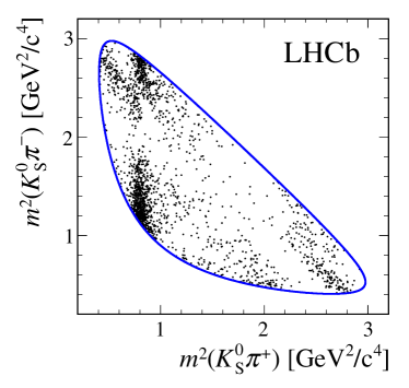
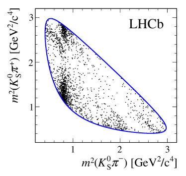
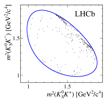
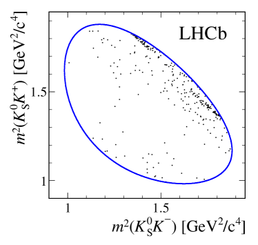
Figure 2: Dalitz plots of long and downstream (left) ${{{B}^{+}}}\rightarrow D{{K}^{+}}$ and (right) ${{{B}^{-}}}\rightarrow D{{K}^{-}}$ candidates for (top) $D\rightarrow{{K}^{0}_{\mathrm{\scriptscriptstyle S}}}{{\pi}^{+}}{{\pi}^{-}}$ and (bottom) $D\rightarrow{{K}^{0}_{\mathrm{\scriptscriptstyle S}}}{{K}^{+}}{{K}^{-}}$ decays in which the reconstructed invariant mass of the ${B}^{\pm}$ candidate is in a region of $\pm 25{\mathrm{\,Me\kern-0.90005ptV\!/}c^{2}}$ around the ${B}^{\pm}$ mass. The narrow region is chosen to obtain high purity, as no background subtraction has been made. The Dalitz coordinates are calculated using the results of a kinematic fit in which the $D$ and ${K}^{0}_{\mathrm{\scriptscriptstyle S}}$ masses are constrained to their known values. The blue lines show the kinematic boundaries of the decays.

The Dalitz plots for ${{B}^{\pm}}\rightarrow D{{K}^{\pm}}$ candidates in a narrow region of $\pm 25{\mathrm{\,Me\kern-1.00006ptV\!/}c^{2}}$ around the ${B}^{\pm}$ mass are shown in Fig. 2, for both $D\rightarrow{{K}^{0}_{\mathrm{\scriptscriptstyle S}}}h^{+}h^{-}$ final states samples. Separate plots are shown for $B^{+}$ and $B^{-}$ decays. The Dalitz coordinates are calculated from the kinematic fit with all mass constraints applied.

In order to determine the parameterisation of the signal and background components that are used in the fit of partitioned regions of the Dalitz plot described in Sect. 6, an extended maximum likelihood fit to the invariant-mass distributions of the ${B}^{\pm}$ candidates is performed, in which the ${{B}^{+}}$ and ${{B}^{-}}$ candidates in all of the Dalitz bins are combined. The invariant mass of each ${B}^{\pm}$ candidate is calculated using the results of a kinematic fit in which the $D$ and ${K}^{0}_{\mathrm{\scriptscriptstyle S}}$ masses are constrained to their known values. The sample is split into ${{B}^{\pm}}\rightarrow D{{K}^{\pm}}$ and ${{B}^{\pm}}\rightarrow D{{\pi}^{\pm}}$ candidates, by $D$ decay mode and by ${K}^{0}_{\mathrm{\scriptscriptstyle S}}$ category. In order to allow sharing of some parameters, the fit is performed simultaneously for all of the above categories. The projections of the fit and the invariant-mass distributions of the selected ${B}^{\pm}$ candidates are shown in Figs. 3 and 4 for $D\rightarrow{{K}^{0}_{\mathrm{\scriptscriptstyle S}}}{{\pi}^{+}}{{\pi}^{-}}$ and $D\rightarrow{{K}^{0}_{\mathrm{\scriptscriptstyle S}}}{{K}^{+}}{{K}^{-}}$ candidates, respectively. The fit range is between 5080${\mathrm{\,Me\kern-1.00006ptV\!/}c^{2}}$ and 5800${\mathrm{\,Me\kern-1.00006ptV\!/}c^{2}}$ in the ${B}^{\pm}$ candidate invariant mass.

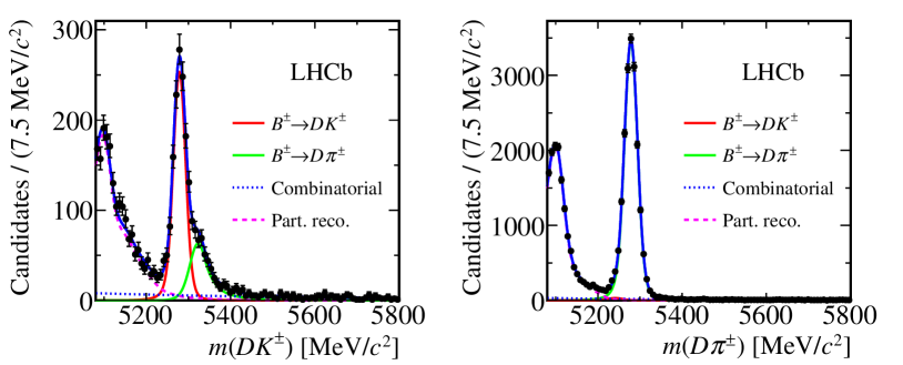
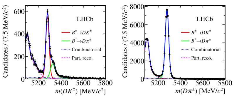
Figure 3: Invariant-mass distributions of (left) ${{B}^{\pm}}\rightarrow D{{K}^{\pm}}$ and (right) ${{B}^{\pm}}\rightarrow D{{\pi}^{\pm}}$ candidates, with $D\rightarrow{{K}^{0}_{\mathrm{\scriptscriptstyle S}}}{{\pi}^{+}}{{\pi}^{-}}$, shown separately for the (top) long and (bottom) downstream ${K}^{0}_{\mathrm{\scriptscriptstyle S}}$ categories. Fit results, including the signal component and background components due to misidentified companions, partially reconstructed decays and combinatorial background, are also shown.

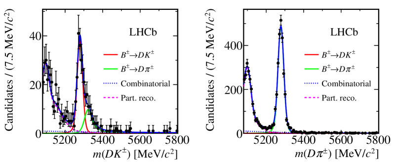
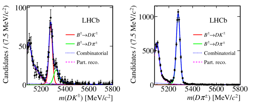
Figure 4: Invariant-mass distributions of (left) ${{B}^{\pm}}\rightarrow D{{K}^{\pm}}$ and (right) ${{B}^{\pm}}\rightarrow D{{\pi}^{\pm}}$ candidates, with $D\rightarrow{{K}^{0}_{\mathrm{\scriptscriptstyle S}}}{{K}^{+}}{{K}^{-}}$, shown separately for the (top) long and (bottom) downstream ${K}^{0}_{\mathrm{\scriptscriptstyle S}}$ categories. Fit results, including the signal component and background components due to misidentified companions, partially reconstructed decays and combinatorial background, are also shown.

The peaks corresponding to actual ${{B}^{\pm}}\rightarrow D{{K}^{\pm}}$ and ${{B}^{\pm}}\rightarrow D{{\pi}^{\pm}}$ candidates are fitted with a sum of two Crystal Ball [47] functions, which are parameterised as

$$\text{CB}(m,\mu,\sigma,\alpha,n)\propto\left\{\begin{array}[]{ll}\exp\left[-\frac{1}{2}\left(\frac{m-\mu}{\sigma}\right)^{2}\right]&\text{if }(m-\mu)/\sigma>-\alpha\\ A\left(B-\frac{m-\mu}{\sigma}\right)^{-n}&\text{otherwise,}\end{array}\right.$$ (8)

where $\alpha>0$, and

$$A =\left(\frac{n}{\alpha}\right)^{n}\exp[-\alpha^{2}/2]\,,$$ (9)

$$B =\frac{n}{\alpha}-\alpha\,.$$ (10)

The sum is implemented such that the Crystal Ball functions have tails pointing in either direction. They share a common width, $\sigma$, and mean, $\mu$. In practice, the signal probability density function (PDF) is defined as

$$f_{\text{signal}}(m,\mu,\sigma,\alpha_{\text{L}} ,n_{\text{L}},\alpha_{\text{R}},n_{\text{R}},f_{\text{CB}})$$

$$=f_{\text{CB}}\cdot\text{CB}(m,\mu,\sigma,\alpha_{\text{L}},n_{\text{L}})+(1-f_{\text{CB}})\cdot\text{CB}(m,\mu,-\sigma,\alpha_{\text{R}},n_{\text{R}}).$$ (11)

The tail parameters, $n_{\text{L},\text{R}}$ and $\alpha_{\text{L},\text{R}}$, are fixed from simulation, while the other parameters are left as free parameters in the fit. Separate tail parameters, $f_{\text{CB}}$, and $\sigma$ are used for long and downstream candidates. Different widths are used for the ${{B}^{\pm}}\rightarrow D{{K}^{\pm}}$ and ${{B}^{\pm}}\rightarrow D{{\pi}^{\pm}}$ channels, with their ratio $r_{\sigma}=\sigma_{DK}/\sigma_{D\pi}$ shared between all categories. The mean is shared among all categories. The yield of ${{B}^{\pm}}\rightarrow D{{\pi}^{\pm}}$ decays in each ${K}^{0}_{\mathrm{\scriptscriptstyle S}}$ and $D$-meson decay category, $N^{\text{cat}}({{B}^{\pm}}\rightarrow D{{\pi}^{\pm}})$, is determined in the fit. Instead of fitting the yield of ${{B}^{\pm}}\rightarrow D{{K}^{\pm}}$ decays directly in each category, it is determined from the ${{B}^{\pm}}\rightarrow D{{\pi}^{\pm}}$ yield in the corresponding category and the ratio

$$\mathcal{R}\equiv\frac{N^{\text{cat}}({{B}^{\pm}}\rightarrow D{{K}^{\pm}})}{{\varepsilon}^{\text{cat}}_{\text{PID}}({{B}^{\pm}}\rightarrow D{{K}^{\pm}})}\bigg{/}\frac{N^{\text{cat}}({{B}^{\pm}}\rightarrow D{{\pi}^{\pm}})}{{\varepsilon}^{\text{cat}}_{\text{PID}}({{B}^{\pm}}\rightarrow D{{\pi}^{\pm}})}\,,$$ (12)

which is a free parameter in the fit. The category-dependent PID efficiencies, ${\varepsilon}^{\text{cat}}_{\text{PID}}({{B}^{\pm}}\rightarrow{D}h^{\pm})$, are taken into account, so that a single $\mathcal{R}$ parameter can be shared between all categories in the fit. How these efficiencies are obtained is described below. As the parameter $\mathcal{R}$ is efficiency corrected, it is equal to the ratio of branching fractions between the ${{B}^{\pm}}\rightarrow D{{K}^{\pm}}$ and ${{B}^{\pm}}\rightarrow D{{\pi}^{\pm}}$ decay modes. The measured ratio is found to be ${\mathcal{R}}=(7.66\pm 0.14)\,\%$, where the uncertainty is statistical only, and this is consistent with the expected value of $(7.8\pm 0.4)\,\%$ [44].

The background consists of random track combinations, partially reconstructed $B$ decays, and ${{B}^{\pm}}\rightarrow Dh^{\pm}$ decays in which the companion has been misidentified. The random track combinations are modelled by an exponential PDF. The slopes of the exponentials are free parameters in the fit to the data. These slopes are independent for each of the ${{B}^{\pm}}\rightarrow D{{\pi}^{\pm}}$ categories, while they are shared for the ${{B}^{\pm}}\rightarrow D{{K}^{\pm}}$ categories to improve the stability of the fit. When these slopes are allowed to be independent, the fit returns results that are statistically compatible.

In the ${{B}^{\pm}}\rightarrow D{{K}^{\pm}}$ sample there is a clear contribution from ${{B}^{\pm}}\rightarrow D{{\pi}^{\pm}}$ decays in which the companion particle is misidentified as a kaon by the RICH system. The rate for ${{B}^{\pm}}\rightarrow D{{K}^{\pm}}$ decays to be misidentified and placed in the ${{B}^{\pm}}\rightarrow D{{\pi}^{\pm}}$ sample is much lower due to the reduced branching fraction. Nevertheless, this contribution is still accounted for in the fit. The yields of these backgrounds are fixed in the fit, using knowledge of misidentification efficiencies and the fitted yields of reconstructed decays with the correct particle hypothesis. The misidentification efficiencies are obtained from large samples of ${{D}^{*\pm}}\rightarrow\kern 1.79993pt\shortstack{{(\rule[2.15277pt]{12.50002pt}{0.51212pt})} \\ [-.7ex] $\kern-1.79993ptD$}{}^{0}\pi^{\pm}$, $\kern 1.79993pt\shortstack{{(\rule[2.15277pt]{12.50002pt}{0.51212pt})} \\ [-.7ex] $\kern-1.79993ptD$}{}^{0}\rightarrow K^{\mp}\pi^{\pm}$ decays. These decays are selected using only kinematic variables in order to provide pure samples of ${{K}^{\mp}}$ and ${{\pi}^{\pm}}$ that are unbiased in the PID variables. The PID efficiency is parameterised as a function of the companion momentum and pseudorapidity, and the charged-particle multiplicity in the event. The calibration sample is weighted so that the distribution of these variables matches that of the candidates in the signal region of the ${B}^{\pm}$ sample, thereby ensuring that the measured PID performance is representative for the samples used in this measurement. The efficiency to identify a kaon correctly is found to be approximately 86 %, while that for a pion is approximately 97 %. The PDFs of the backgrounds due to misidentified companion particles are determined using data. As an example, consider the case of true ${{B}^{\pm}}\rightarrow D{{\pi}^{\pm}}$ decays misidentified as ${{B}^{\pm}}\rightarrow D{{K}^{\pm}}$ candidates. The sPlot method [48] is used on the ${{B}^{\pm}}\rightarrow D{{\pi}^{\pm}}$ sample in order to isolate the contribution from the signal decays. The ${B}^{\pm}$ invariant mass is then calculated using the kaon mass hypothesis for the companion pion, and weighting by PID efficiencies in order to properly reproduce the kinematic properties of pions misidentified as kaons in the signal ${{B}^{\pm}}\rightarrow D{{K}^{\pm}}$ sample. The weighted distribution is fitted with a sum of two Crystal Ball shapes. The fitted parameters are subsequently fixed in the fit to the ${B}^{\pm}$ invariant-mass spectrum, with the procedure applied separately for long and downstream candidates. An analogous approach is used to determine the shape of the misidentified ${{B}^{\pm}}\rightarrow D{{K}^{\pm}}$ contribution in the ${{B}^{\pm}}\rightarrow D{{\pi}^{\pm}}$ sample.

Partially reconstructed $b$-hadron decays contaminate the sample predominantly at invariant masses smaller than that of the signal peak. These decays contain an unreconstructed pion or photon, which predominantly comes from an intermediate resonance. There are contributions from $B^{0}\rightarrow D^{*\pm}h^{\mp}$ and $B^{\pm}\rightarrow D^{*0}h^{\pm}$ decays in all channels (denoted as ${B}\rightarrow{D}^{*}h^{\pm}$ decays), while $B^{\pm}\rightarrow{D}\rho^{\pm}$ and $B^{\pm}\rightarrow{D}{{K}^{*\pm}}$ decays contribute to the ${{B}^{\pm}}\rightarrow D{{\pi}^{\pm}}$ and ${{B}^{\pm}}\rightarrow D{{K}^{\pm}}$ channels, respectively. In the ${{B}^{\pm}}\rightarrow D{{K}^{\pm}}$ channels there is also a contribution from ${{B}^{0}_{s}}\rightarrow{{\kern 1.99997pt\overline{\kern-1.99997ptD}{}}{}^{0}}\pi^{+}{{K}^{-}}$ (${{\kern 1.79993pt\overline{\kern-1.79993ptB}{}}{}^{0}_{s}}\rightarrow{{D}^{0}}\pi^{-}{{K}^{+}}$) decays where the charged pion is not reconstructed. The invariant-mass distributions of these backgrounds depend on the spin and mass of the missing particle, as described in Ref. [49]. The shape of the background from ${B}^{0}_{s}$ decays is based on the results of Ref. [50]. Additionally, each of the above backgrounds of ${{B}^{\pm}}\rightarrow D{{\pi}^{\pm}}$ decays can contribute in the ${{B}^{\pm}}\rightarrow D{{K}^{\pm}}$ channels if the pion is misidentified. The inverse contribution is negligible and is neglected. The shapes for the decays in which a pion is misidentified as a kaon are parameterised with semi-empirical PDFs formed from sums of Gaussian and error functions. The parameters of these backgrounds are fixed to the results of fits to data from two-body $D$ decays [49], where they were obtained with a much larger data sample. However, the width of the resolution function and a shift along the ${B}^{\pm}$ mass are allowed to differ in order to accommodate small differences between the $D$ decay modes.

In each of the ${{B}^{\pm}}\rightarrow D{{\pi}^{\pm}}$ channels, the total yield of the partially reconstructed background is fitted independently. The relative amount of each ${B}\rightarrow{D}^{*}\pi^{\mp}$ mode is fixed from efficiencies obtained from simulation and known branching fractions, while the fraction of $B^{\pm}\rightarrow{D}\rho^{\pm}$ decays is left free. In the ${{B}^{\pm}}\rightarrow D{{K}^{\pm}}$ channels, the yield of the ${{B}^{0}_{s}}\rightarrow{{\kern 1.99997pt\overline{\kern-1.99997ptD}{}}{}^{0}}\pi^{+}{{K}^{-}}$ background is fixed relative to the corresponding ${{B}^{\pm}}\rightarrow D{{\pi}^{\pm}}$ yield, using efficiencies from simulation and the known branching fraction. The total yield of the remaining partially reconstructed backgrounds is expressed via a single fraction, $\mathcal{R}_{{D}{K}/{D}\pi}^{\text{low}}$, relative the ${{B}^{\pm}}\rightarrow D{{\pi}^{\pm}}$ yields. It is free in the fit, and common to all channels after taking into account the different particle-identification efficiencies. The relative amount of each ${B}\rightarrow{D}^{*}{K}^{\mp}$ mode is fixed using efficiencies from simulation and known branching fractions, while the fraction of $B^{\pm}\rightarrow{D}{{K}^{*}}^{\pm}$ decays is fixed using the results of Ref. [49]. The yields of the partially reconstructed modes with a companion pion misidentified as a kaon are fixed via the known PID efficiencies, based on the fitted yield of the partially reconstructed backgrounds in the corresponding ${{B}^{\pm}}\rightarrow D{{\pi}^{\pm}}$ channel.

In the ${{B}^{\pm}}\rightarrow D{{\pi}^{\pm}}$ channels, a total signal yield of approximately $56\,100$ ($7750$) is found in the signal region 5249–5319${\mathrm{\,Me\kern-1.00006ptV\!/}c^{2}}$ of the $D\rightarrow{{K}^{0}_{\mathrm{\scriptscriptstyle S}}}{{\pi}^{+}}{{\pi}^{-}}$ ($D\rightarrow{{K}^{0}_{\mathrm{\scriptscriptstyle S}}}{{K}^{+}}{{K}^{-}}$) channel, $31\,\%$ ($32\,\%$) of which are in the long ${K}^{0}_{\mathrm{\scriptscriptstyle S}}$ category. The purity in the signal region is found to be $98.4\,\%$ ($97.7\,\%$), with the dominant background being combinatorial. In the ${{B}^{\pm}}\rightarrow D{{K}^{\pm}}$ channels, a total signal yield of approximately $3900$ ($530$) is found in the signal region of the $D\rightarrow{{K}^{0}_{\mathrm{\scriptscriptstyle S}}}{{\pi}^{+}}{{\pi}^{-}}$ ($D\rightarrow{{K}^{0}_{\mathrm{\scriptscriptstyle S}}}{{K}^{+}}{{K}^{-}}$) channel, again finding $31\,\%$ ($32\,\%$) of the candidates in the long ${K}^{0}_{\mathrm{\scriptscriptstyle S}}$ category. The purity in the signal region is found to be $81\,\%$. The dominant background is from misidentified ${{B}^{\pm}}\rightarrow D{{\pi}^{\pm}}$ decays, which accounts for $66\,\%$ of the background in the signal region. Equal amounts of combinatorial background and partially reconstructed decays, predominantly including a misidentified companion pion, make up the remaining background.

5 Event selection and yield determination for ${\shortstack{{(\rule[2.15277pt]{17.50002pt}{0.51212pt})} \\ [-.3ex] $B$}{}\rightarrow{{D}^{*\pm}}\mu^{\mp}\shortstack{{(\rule[2.15277pt]{12.50002pt}{0.51212pt})} \\ [-.3ex] $\nu$}\!_{\mu}}$ decays

A sample of $\kern 1.79993pt\shortstack{{(\rule[2.15277pt]{12.50002pt}{0.51212pt})} \\ [-.7ex] $\kern-1.79993ptB$}{}\!\rightarrow{{D}^{*\pm}}\mu^{\mp}\shortstack{{(\rule[2.15277pt]{10.00002pt}{0.51212pt})} \\ [-.7ex] $\nu$}{}_{\!\!\mu}X$, ${{D}^{*\pm}}\rightarrow\kern 1.79993pt\shortstack{{(\rule[2.15277pt]{12.50002pt}{0.51212pt})} \\ [-.7ex] $\kern-1.79993ptD$}{}{{\pi}^{\pm}}$, $\kern 1.79993pt\shortstack{{(\rule[2.15277pt]{12.50002pt}{0.51212pt})} \\ [-.7ex] $\kern-1.79993ptD$}{}\rightarrow{{K}^{0}_{\mathrm{\scriptscriptstyle S}}}h^{+}h^{-}$ decays is used to determine the quantities $F_{i}$, defined in Eq. (5), as the expected fractions of ${D}^{0}$ decays falling into the $i$th Dalitz plot bin, taking into account the efficiency profile of the signal decay. The semileptonic decay of the $B$ meson and the strong-interaction decay of the ${D}^{*\pm}$ meson allow the flavour of the ${D}^{0}$ meson to be determined from the charges of the muon and the soft pion from the ${D}^{*\pm}$ decay. This particular decay chain, involving a flavour-tagged ${D}^{0}$ decay, is chosen due to its high yield, low background level, and low mistag probability. The selection requirements are chosen to minimise changes to the efficiency profile with respect to those associated with the ${{B}^{\pm}}\rightarrow D{{K}^{\pm}}$ channels.

The selection is identical to that applied in Ref. [9], except for a tighter requirement on the significance of the ${D}^{0}$ flight distance that helps to suppress backgrounds from charmless $B$ decays. To improve the resolution of the distribution of candidates across the Daltiz plot, the $B$-decay chain is refitted [43] with the ${D}^{0}$ and ${K}^{0}_{\mathrm{\scriptscriptstyle S}}$ candidates constrained to their known masses. An additional fit, in which only the ${K}^{0}_{\mathrm{\scriptscriptstyle S}}$ mass is constrained, is performed to improve the ${D}^{0}$ and ${D}^{*\pm}$ mass resolution in the invariant-mass fit used to determine signal yields.

The invariant mass of the ${D}^{0}$ candidate, $m({{K}^{0}_{\mathrm{\scriptscriptstyle S}}}h^{+}h^{-})$, and the invariant-mass difference, $\Delta m\equiv m({{K}^{0}_{\mathrm{\scriptscriptstyle S}}}h^{+}h^{-}{{\pi}^{\pm}})-m({{K}^{0}_{\mathrm{\scriptscriptstyle S}}}h^{+}h^{-})$, are fitted simultaneously to determine the signal yields. This two-dimensional parameterisation allows the yield of selected candidates to be measured in three categories: true ${{D}^{*\pm}}$ candidates (signal), candidates containing a true ${D}^{0}$ meson but random soft pion (RSP) and candidates formed from random track combinations that fall within the fit range (combinatorial background). Background contributions from real ${D}^{*\pm}$ decays paired with a random $\mu$ are determined to be negligible by selecting pairs of ${{D}^{*\pm}}$ mesons and $\mu^{\pm}$ with the same charge.

An example projection of $m({{K}^{0}_{\mathrm{\scriptscriptstyle S}}}{{\pi}^{+}}{{\pi}^{-}})$ and $\Delta m$ is shown in Fig. 5. The result of a two-dimensional extended, unbinned, maximum likelihood fit is superimposed. The fit is performed simultaneously for the two ${D}^{0}$ final states and the two ${K}^{0}_{\mathrm{\scriptscriptstyle S}}$ categories with some parameters allowed to be independent between categories. Candidates selected from data recorded in 2015 and 2016 are fitted separately, in order to accommodate different trigger threshold settings that result in slightly different Dalitz plot efficiency profiles. The fit region is defined by $1830<m({{K}^{0}_{\mathrm{\scriptscriptstyle S}}}h^{+}h^{-})<1910{\mathrm{\,Me\kern-1.00006ptV\!/}c^{2}}$ and $139.5<\Delta m<153.0{\mathrm{\,Me\kern-1.00006ptV\!/}c^{2}}$. Within this $m({{K}^{0}_{\mathrm{\scriptscriptstyle S}}}h^{+}h^{-})$ range, the $\Delta m$ resolution does not vary significantly.

The signal is parameterised in $\Delta m$ with a sum of two Crystal Ball functions, as for the ${{B}^{\pm}}\rightarrow Dh^{\pm}$ signal. The mean, $\mu$, is shared between all categories, while the other parameters are different for long and downstream candidates. The tail parameters are fixed from simulation. The combinatorial and RSP backgrounds are both parameterised with an empirical model given by

$$f(\Delta m;\Delta m_{0},x,p_{1},p_{2})=\left[1-\exp\left(-\frac{\Delta m-\Delta m_{0}}{x}\right)\right]\left({\frac{\Delta m}{\Delta m_{0}}}\right)^{p_{1}}+p_{2}\left(\frac{\Delta m}{\Delta m_{0}}-1\right)$$ (13)

for $\Delta m-\Delta m_{0}>0$ and $f(\Delta m)=0$ otherwise, where $\Delta m_{0}$, $x$, $p_{1}$, and $p_{2}$ are free parameters. The parameter $\Delta m_{0}$, which describes the kinematic threshold for a ${{D}^{*\pm}}\rightarrow\kern 1.79993pt\shortstack{{(\rule[2.15277pt]{12.50002pt}{0.51212pt})} \\ [-.7ex] $\kern-1.79993ptD$}{}{}^{0}\pi^{\pm}$ decay, is shared in all data categories and for both the combinatorial and RSP shapes. The remaining parameters are determined separately for $D\rightarrow{{K}^{0}_{\mathrm{\scriptscriptstyle S}}}{{\pi}^{+}}{{\pi}^{-}}$ and $D\rightarrow{{K}^{0}_{\mathrm{\scriptscriptstyle S}}}{{K}^{+}}{{K}^{-}}$ candidates.

In the $m({{K}^{0}_{\mathrm{\scriptscriptstyle S}}}h^{+}h^{-})$ fit, all of the parameters in the signal and RSP PDFs are constrained to be the same as both describe a true ${D}^{0}$ candidate. These are also fitted with a sum of two Crystal Ball functions, with the tail parameters fixed from simulation. The parameters are fitted separately for the $D\rightarrow{{K}^{0}_{\mathrm{\scriptscriptstyle S}}}{{\pi}^{+}}{{\pi}^{-}}$ and $D\rightarrow{{K}^{0}_{\mathrm{\scriptscriptstyle S}}}{{K}^{+}}{{K}^{-}}$ shapes, due to the different phase space available in the ${D}^{0}$ decay. The combinatorial background is parameterised by an exponential function in $m({{K}^{0}_{\mathrm{\scriptscriptstyle S}}}h^{+}h^{-})$.

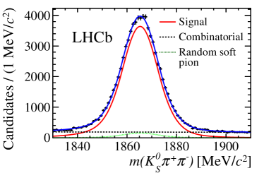
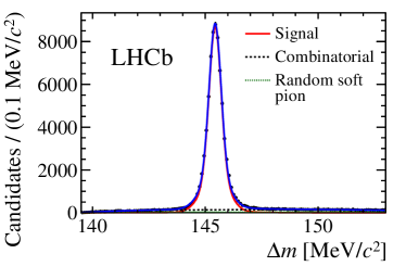
Figure 5: Result of the simultaneous fit to $\kern 1.79993pt\shortstack{{(\rule[2.15277pt]{12.50002pt}{0.51212pt})} \\ [-.7ex] $\kern-1.79993ptB$}{}\!\rightarrow{{D}^{*\pm}}\mu^{\mp}\shortstack{{(\rule[2.15277pt]{10.00002pt}{0.51212pt})} \\ [-.7ex] $\nu$}{}_{\!\!\mu}$, ${{D}^{*}}^{\pm}\rightarrow\kern 1.79993pt\shortstack{{(\rule[2.15277pt]{12.50002pt}{0.51212pt})} \\ [-.7ex] $\kern-1.79993ptD$}{}^{0}(\rightarrow{{K}^{0}_{\mathrm{\scriptscriptstyle S}}}{{\pi}^{+}}{{\pi}^{-}}){{\pi}^{\pm}}$ decays with downstream ${K}^{0}_{\mathrm{\scriptscriptstyle S}}$ candidates, in 2016 data. The projections of the fit result are shown for (left) $m({{K}^{0}_{\mathrm{\scriptscriptstyle S}}}{{\pi}^{+}}{{\pi}^{-}})$ and (right) $\Delta m$. The (blue) total fit PDF is the sum of components describing (solid red) signal, (dashed black) combinatorial background and (dotted green) random soft pion background.

A total signal yield of approximately 113 000 (15 000) $D\rightarrow{{K}^{0}_{\mathrm{\scriptscriptstyle S}}}{{\pi}^{+}}{{\pi}^{-}}$ ($D\rightarrow{{K}^{0}_{\mathrm{\scriptscriptstyle S}}}{{K}^{+}}{{K}^{-}}$) decays is obtained. This is approximately 25 times larger than the ${{B}^{\pm}}\rightarrow D{{K}^{\pm}}$ yield. In the range surrounding the signal peaks, defined as 1840–1890 (1850–1880)${\mathrm{\,Me\kern-1.00006ptV\!/}c^{2}}$ in $m({{K}^{0}_{\mathrm{\scriptscriptstyle S}}}{{\pi}^{+}}{{\pi}^{-}})$ ($m({{K}^{0}_{\mathrm{\scriptscriptstyle S}}}{{K}^{+}}{{K}^{-}})$) and 143.9–146.9${\mathrm{\,Me\kern-1.00006ptV\!/}c^{2}}$ in $\Delta m$, the background components account for 2–5 % of the yield depending on the category.

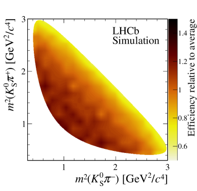
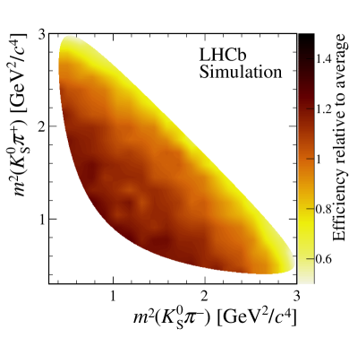
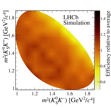
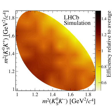
Figure 6: Example efficiency profiles of (left) ${{B}^{\pm}}\rightarrow D{{\pi}^{\pm}}$ and (right) $\kern 1.79993pt\shortstack{{(\rule[2.15277pt]{12.50002pt}{0.51212pt})} \\ [-.7ex] $\kern-1.79993ptB$}{}\!\rightarrow{{D}^{*\pm}}\mu^{\mp}\shortstack{{(\rule[2.15277pt]{10.00002pt}{0.51212pt})} \\ [-.7ex] $\nu$}{}_{\!\!\mu}X$ decays in the simulation. The top (bottom) plots are for $D\rightarrow{{K}^{0}_{\mathrm{\scriptscriptstyle S}}}{{\pi}^{+}}{{\pi}^{-}}$ ($D\rightarrow{{K}^{0}_{\mathrm{\scriptscriptstyle S}}}{{K}^{+}}{{K}^{-}}$) decays. These plots refer to downstream ${K}^{0}_{\mathrm{\scriptscriptstyle S}}$ candidates under 2016 data taking conditions. The normalisation is chosen so that the average over the Dalitz plot is unity.

The two-dimensional fit in $m({{K}^{0}_{\mathrm{\scriptscriptstyle S}}}h^{+}h^{-})$ and $\Delta m$ of the $\kern 1.79993pt\shortstack{{(\rule[2.15277pt]{12.50002pt}{0.51212pt})} \\ [-.7ex] $\kern-1.79993ptB$}{}\!\rightarrow{{D}^{*\pm}}\mu^{\mp}\shortstack{{(\rule[2.15277pt]{10.00002pt}{0.51212pt})} \\ [-.7ex] $\nu$}{}_{\!\!\mu}X$ decay is repeated in each Dalitz plot bin with all of the PDF parameters fixed, resulting in a raw control-mode yield, $R_{i}$, for each bin $i$. The measured $R_{i}$ are not equivalent to the $F_{i}$ fractions required to determine the $C\!P$ parameters due to unavoidable differences from selection criteria in the efficiency profiles of the signal and control modes. Examples of the efficiency profiles from simulation of the downstream candidates in 2016 data are shown in Fig. 6. For each Dalitz plot bin $i$ a correction factor $\xi_{i}$ is determined to account for these efficiency differences, defined as

$$\xi_{i}\equiv\frac{\int_{i}dm^{2}_{-}\,dm^{2}_{+}\,|A_{D}(m^{2}_{-},m^{2}_{+})|^{2}\,\eta(m^{2}_{-},m^{2}_{+})_{D\pi}}{\int_{i}dm^{2}_{-}\,dm^{2}_{+}\,|A_{D}(m^{2}_{-},m^{2}_{+})|^{2}\,\eta(m^{2}_{-},m^{2}_{+})_{{{D}^{*}}\!\mu}},$$ (14)

where $\eta(m^{2}_{-},m^{2}_{+})_{D\pi}$ and $\eta(m^{2}_{-},m^{2}_{+})_{{{D}^{*}}\!\mu}$ are the efficiency profiles of the ${{B}^{\pm}}\rightarrow D{{\pi}^{\pm}}$ and $\kern 1.79993pt\shortstack{{(\rule[2.15277pt]{12.50002pt}{0.51212pt})} \\ [-.7ex] $\kern-1.79993ptB$}{}\!\rightarrow{{D}^{*\pm}}\mu^{\mp}\shortstack{{(\rule[2.15277pt]{10.00002pt}{0.51212pt})} \\ [-.7ex] $\nu$}{}_{\!\!\mu}X$ decays, respectively, and are determined from simulation. The ${{B}^{\pm}}\rightarrow D{{\pi}^{\pm}}$ decay mode is used rather than ${{B}^{\pm}}\rightarrow D{{K}^{\pm}}$ as the simulation is more easily compared to the data, due to the larger decay rate and the smaller interference between ${{B}^{\pm}}\rightarrow{{D}^{0}}\pi^{\pm}$ and ${{B}^{\pm}}\rightarrow{{\kern 1.99997pt\overline{\kern-1.99997ptD}{}}{}^{0}}\pi^{\pm}$ decays, compared to in the ${{B}^{\pm}}\rightarrow D{{K}^{\pm}}$ decay mode. It is verified using simulation that the efficiency profiles of the ${{B}^{\pm}}\rightarrow D{{\pi}^{\pm}}$ and ${{B}^{\pm}}\rightarrow D{{K}^{\pm}}$ decays are the same. The simulated events are generated with a flat distribution across the ${D}\rightarrow{{K}^{0}_{\mathrm{\scriptscriptstyle S}}}h^{+}h^{-}$ phase space; hence the distribution of simulated events after triggering, reconstruction and selection is directly proportional to the efficiency profile. The amplitude models used to determine the Dalitz plot intensity for the correction factor are those from Ref. [23] and Ref. [24] for the $D\rightarrow{{K}^{0}_{\mathrm{\scriptscriptstyle S}}}{{\pi}^{+}}{{\pi}^{-}}$ and $D\rightarrow{{K}^{0}_{\mathrm{\scriptscriptstyle S}}}{{K}^{+}}{{K}^{-}}$ decays, respectively. The amplitude models provide a description of the intensity distribution over the Dalitz plot and introduce no significant model dependence into the analysis. The $F_{i}$ values can be determined via the relation $F_{i}=h^{\prime}\xi_{i}R_{i}$, where $h^{\prime}$ is a normalisation factor such that the sum of all $F_{i}$ is unity. The $F_{i}$ values are determined separately for each year of data taking and ${K}^{0}_{\mathrm{\scriptscriptstyle S}}$ category and are then combined in the fractions observed in the ${{B}^{\pm}}\rightarrow D{{\pi}^{\pm}}$ signal region in data. This method of determining the $F_{i}$ parameters is preferable to using solely the amplitude models and ${{B}^{\pm}}\rightarrow D{{\pi}^{\pm}}$ simulated events, since the method is data-driven. The amplitude models and simulation data enter the correction factor as a ratio, and thus imperfections in the simulation and the model cancel at first order. The average correction factor over all bins is approximately $2\,\%$ from unity and the largest correction factor is within $7\,\%$. Uncertainties on these correction factors are driven by the size of the simulation samples and are of a similar size as the corrections themselves.

6 Dalitz plot fit to determine the $C\!P$-violating parameters $x_{\pm}$ and $y_{\pm}$

The Dalitz plot fit is used to measure the $C\!P$-violating parameters $x_{\pm}$ and $y_{\pm}$, as introduced in Sect. 2. Following Eq. (4), these parameters are determined from the populations of the ${{B}^{+}}$ and ${{B}^{-}}$ Dalitz plot bins, given the external information of the $c_{i}$ and $s_{i}$ parameters from CLEO-c data and the values of $F_{i}$ from the semileptonic control decay modes. Although the absolute numbers of ${{B}^{+}}$ and ${{B}^{-}}$ decays integrated over the $D$ Dalitz plot have some dependence on $x_{\pm}$ and $y_{\pm}$, the sensitivity gained compared to using just the relations in Eq. (4) is negligible [51] given the available sample size. Consequently, as stated previously, the integrated yields are not used to provide information on $x_{\pm}$ and $y_{\pm}$ and the analysis is insensitive to $B$ meson production and detection asymmetries.

A simultaneous fit is performed on the ${{B}^{\pm}}\rightarrow Dh^{\pm}$ data, split into the two $B$ charges, the two ${K}^{0}_{\mathrm{\scriptscriptstyle S}}$ categories, the ${{B}^{\pm}}\rightarrow D{{K}^{\pm}}$ and ${{B}^{\pm}}\rightarrow D{{\pi}^{\pm}}$ candidates, and the two $D\rightarrow{{K}^{0}_{\mathrm{\scriptscriptstyle S}}}h^{+}h^{-}$ final states. The invariant mass of each ${B}^{\pm}$ candidate is calculated using the results of a kinematic fit in which the $D$ and ${K}^{0}_{\mathrm{\scriptscriptstyle S}}$ masses are constrained to their known values. Each category is then divided into the Dalitz plot bins shown in Fig. 1, where there are 16 bins for $D\rightarrow{{K}^{0}_{\mathrm{\scriptscriptstyle S}}}{{\pi}^{+}}{{\pi}^{-}}$ and 4 bins for $D\rightarrow{{K}^{0}_{\mathrm{\scriptscriptstyle S}}}{{K}^{+}}{{K}^{-}}$. The ${{B}^{\pm}}\rightarrow D{{K}^{\pm}}$ and ${{B}^{\pm}}\rightarrow D{{\pi}^{\pm}}$ samples are fitted simultaneously because the yield of ${{B}^{\pm}}\rightarrow D{{\pi}^{\pm}}$ signal in each Dalitz plot bin is used to determine the yield of misidentified candidates in the corresponding ${{B}^{\pm}}\rightarrow D{{K}^{\pm}}$ Dalitz plot bin. The PDF parameters for both the signal and background invariant-mass distributions are fixed to the values determined in the invariant-mass fit described in Sect. 4. The ${{B}^{\pm}}$ mass range is reduced to 5150–5800${\mathrm{\,Ge\kern-1.00006ptV\!/}c^{2}}$ to avoid the need of a detailed description of the shape of the partially reconstructed background. The yields of signal candidates for each bin in the ${{B}^{\pm}}\rightarrow D{{\pi}^{\pm}}$ sample are free parameters. In each of the ${{B}^{\pm}}\rightarrow D{{K}^{\pm}}$ channels, the total yield integrated over the Dalitz plot is a free parameter. The fractional yields in each bin are defined using the expressions for the Dalitz plot distribution in terms of $x_{\pm},\,y_{\pm},\,F_{i},\,c_{i}$, and $s_{i}$ in Eq. (4), where the $x_{\pm}$ and $y_{\pm}$ parameters are free and the values of $F_{i}$ are Gaussian-constrained within their uncertainties. The values of $c_{i}$ and $s_{i}$ are fixed to their central values, which is taken into account as a source of systematic uncertainty. The yields of the component due to ${{B}^{\pm}}\rightarrow D{{\pi}^{\pm}}$ decays, where the companion has been misidentified as a kaon, are fixed in each ${{B}^{\pm}}\rightarrow D{{K}^{\pm}}$ bin, relative to the yield in the corresponding ${{B}^{\pm}}\rightarrow D{{\pi}^{\pm}}$ bin, using the known PID efficiencies. A component for misidentified ${{B}^{\pm}}\rightarrow D{{K}^{\pm}}$ decays in the ${{B}^{\pm}}\rightarrow D{{\pi}^{\pm}}$ channels is not included, as it is found to contribute less than $0.5\%$ of the yield in the signal region in the global fit described in Sect. 4. The total yield of the partially reconstructed ${B}^{\pm}$ and ${B}^{0}$ backgrounds is fitted in each bin, using the same shape in all bins, with the fractions of each component taken from the global fit. The total yield of the ${{B}^{0}_{s}}\rightarrow{{\kern 1.99997pt\overline{\kern-1.99997ptD}{}}{}^{0}}{{\pi}^{+}}{{K}^{-}}$ (${{\kern 1.79993pt\overline{\kern-1.79993ptB}{}}{}^{0}_{s}}\rightarrow{{D}^{0}}{{\pi}^{-}}{{K}^{+}}$) background is fixed in each channel, using the results of the global fit. The yield in each bin is then fixed from the $F_{i}$ parameters, using the known Dalitz distribution of ${{\kern 1.99997pt\overline{\kern-1.99997ptD}{}}{}^{0}}({{D}^{0}})\rightarrow{{K}^{0}_{\mathrm{\scriptscriptstyle S}}}h^{+}h^{-}$ decays. The separate treatment of the partially reconstructed background from ${B}^{0}_{s}$ decays is necessary due to the significantly different Dalitz distribution, arising because only a ${\kern 1.99997pt\overline{\kern-1.99997ptD}{}}{}^{0}$ meson is produced along with a ${K}^{-}$ meson, while for the remaining modes, the $D$ meson is either a ${D}^{0}$ meson or an admixture where the ${\kern 1.99997pt\overline{\kern-1.99997ptD}{}}{}^{0}$ component is $r_{B}$-suppressed. The yield of the combinatorial background in each bin is a free parameter. In bins in which an auxiliary fit determines the yield of the partially reconstructed or combinatorial background to be negligible, the corresponding yields are set to zero to facilitate the calculation of the covariance matrix [52, 53].

A large ensemble of pseudoexperiments is performed to validate the fit procedure. In each pseudoexperiment the numbers and distributions of signal and background candidates are generated according to the expected distribution in data, and the full fit procedure is then executed. The input values for $x_{\pm}$ and $y_{\pm}$ correspond to $\gamma=70^{\circ}$, $r_{B}=0.1$, and $\delta_{B}=130^{\circ}$. The uncertainties determined by the fit to data are consistent with the size of the uncertainties determined by the pseudoexperiments. Small biases are observed in the central values and are due to the low event yields in some of the bins. These biases are observed to decrease in simulated experiments of larger size. The central values are corrected for the biases and a systematic uncertainty is assigned, as described in Sect. 7.

The $C\!P$ parameters obtained from the fit are

$$x_{-} =(\phantom{-}9.0\pm 1.7)\times 10^{-2}\,,$$

$$y_{-} =(\phantom{-}2.1\pm 2.2)\times 10^{-2}\,,$$

$$x_{+} =(-7.7\pm 1.9)\times 10^{-2}\,,$$

$$y_{+} =(-1.0\pm 1.9)\times 10^{-2}\,,$$

where the uncertainties are statistical only. The correlation matrix is shown in Table 1. The total ${{B}^{\pm}}\rightarrow D{{K}^{\pm}}$ yields in the signal region, where the invariant mass of the $B$ candidate is in the interval 5249–5319${\mathrm{\,Me\kern-1.00006ptV\!/}c^{2}}$, are shown in Table 2.

Table 1: Statistical correlation matrix for the fit to data.

	$\phantom{-}x_{-}$	$\phantom{-}y_{-}$	$\phantom{-}x_{+}$	$\phantom{-}y_{+}$
$x_{-}$	$\phantom{-}1$	$-0.21$	$\phantom{-}0.05$	$\phantom{-}0.00$
$y_{-}$		$\phantom{-}1$	$-0.01$	$\phantom{-}0.02$
$x_{+}$			$\phantom{-}1$	$\phantom{-}0.02$
$y_{+}$				$\phantom{-}1$

Table 2: Fit results for the total ${{B}^{\pm}}\rightarrow{D}{{K}^{\pm}}$ yields in the signal region, where the invariant mass of the $B$ candidate is in the interval 5249–5319${\mathrm{\,Me\kern-1.00006ptV\!/}c^{2}}$, integrated over the Dalitz plots.

	${{{B}^{-}}}\rightarrow{D}{{K}^{-}}$			${{{B}^{+}}}\rightarrow{D}{{K}^{+}}$
	Long	Downstream		Long	Downstream
${D}\rightarrow{{K}^{0}_{\mathrm{\scriptscriptstyle S}}}{{\pi}^{+}}{{\pi}^{-}}$	$602\pm 26$	$1\,315\pm 39$		$606\pm 26$	$1\,334\pm 39$
${D}\rightarrow{{K}^{0}_{\mathrm{\scriptscriptstyle S}}}{{K}^{+}}{{K}^{-}}$	$\phantom{6}92\pm 10$	$\phantom{1\,}189\pm 15$		$\phantom{6}82\pm 10$	$\phantom{1\,}193\pm 15$

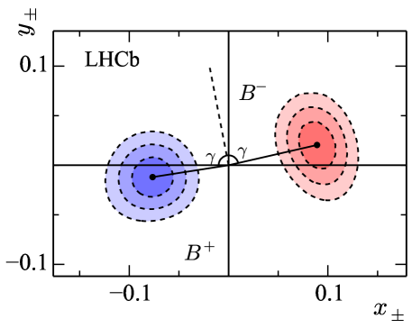
Figure 7: Confidence levels at 68.2%, 95.5% and 99.7% probability for $(x_{+},y_{+})$ and $(x_{-},y_{-})$ as measured in $B^{\pm}\rightarrow DK^{\pm}$ decays (statistical uncertainties only). The parameters $(x_{+},y_{+})$ relate to ${{B}^{+}}$ decays and $(x_{-},y_{-})$ refer to ${{B}^{-}}$ decays. The black dots show the central values obtained in the fit.

The measured values of $(x_{\pm},y_{\pm})$ from the fit to data are displayed in Fig. 7, along with their likelihood contours, corresponding to statistical uncertainties only. The systematic uncertainties are discussed in the next section. The two vectors defined by the coordinates $(x_{-},y_{-})$ and $(x_{+},y_{+})$ are not consistent with zero magnitude and they have a non-zero opening angle. Therefore the data sample exhibits the expected features of $C\!P$ violation. The opening angle is equal to $2\gamma$, as illustrated in Fig. 7.

In order to assess the goodness of fit, and to demonstrate that the equations in $(x_{\pm},y_{\pm})$ provide a good description of data, an alternative fit is performed where the ${{B}^{\pm}}\rightarrow D{{K}^{\pm}}$ yields are measured independently in each bin. In Fig. 8 (left) the obtained yields are compared with the yields predicted from the values of $(x_{\pm},y_{\pm})$ obtained in the default fit. The yields from the direct fit agree with the prediction with a $p$-value of 0.33. In Fig. 8 (right) the difference $N_{{{B}^{+}}}^{i}-N_{{{B}^{-}}}^{-i}$ in each bin is calculated using the results of the direct fit of the ${{B}^{\pm}}\rightarrow D{{K}^{\pm}}$ yields. This distribution is compared to that predicted by the central $(x_{\pm},y_{\pm})$ values. The measured yield differences are compatible with the prediction with a $p$-value of 0.58. In addition, data are fitted with the assumption of no $C\!P$ violation by enforcing $x_{+}=x_{-}\equiv x_{0}$ and $y_{+}=y_{-}\equiv y_{0}$. The obtained $x_{0}$ and $y_{0}$ values are used to determine the predicted values of $N_{{{B}^{+}}}^{i}-N_{{{B}^{-}}}^{-i}$, which are also shown in Fig. 8 (right). This prediction is not zero because the $B$ meson production and various detection effects can induce a global asymmetry in the measured yields. The comparison of the data to this hypothesis yields a $p$-value of $1\times 10^{-6}$, which strongly disfavours the $C\!P$-conserving hypothesis.

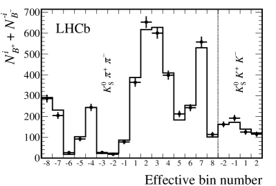
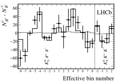
Figure 8: (Left) Comparison of total signal yields from the direct fit (points) to those calculated from the central values of $x_{\pm}$ and $y_{\pm}$ (solid line). The yields are given for the effective bin: $+i$ for ${{B}^{+}}$ and $-i$ for ${{B}^{-}}$, and summed over $B$ charge and ${{K}^{0}_{\mathrm{\scriptscriptstyle S}}}$ decay category. (Right) Comparison of the difference between the ${{B}^{+}}$ and ${{B}^{-}}$ yield obtained in the direct fit for each effective bin (points), the prediction from the central values of $x_{\pm}$ and $y_{\pm}$ (solid line), and the prediction assuming no $C\!P$ violation (dotted line).

7 Systematic uncertainties

Systematic uncertainties on the measurements of the $x_{\pm}$ and $y_{\pm}$ parameters are evaluated and are presented in Table 3. The source of each systematic uncertainty is described below. The systematic uncertainties are generally determined from an ensemble of pseudoexperiments where the simulated data are generated in an alternative configuration and fitted with the default method. The mean shifts in the fitted values of $x_{\pm}$ and $y_{\pm}$ in comparison to their input values are taken as the systematic uncertainty.

Table 3: Summary of uncertainties for the parameters $x_{\pm}$ and $y_{\pm}$. The various sources of systematic uncertainties are described in the main text. All entries are given in multiples of $10^{-2}$.

Source	$\quad x_{-}\quad$	$\quad y_{-}\quad$	$\quad x_{+}\quad$	$\quad y_{+}\quad$
Statistical	1.7	2.2	1.9	1.9
Strong phase measurements	0.4	1.1	0.4	0.9
Efficiency corrections	0.6	0.2	0.6	0.1
Mass fit PDFs	0.2	0.3	0.2	0.3
Different mis-ID shape over Dalitz plot	0.2	0.1	0.1	0.1
Different low mass shape over Dalitz plot	0.1	0.2	0.1	0.1
Uncertainty on ${{B}^{0}_{s}}\rightarrow{{\kern 1.99997pt\overline{\kern-1.99997ptD}{}}{}^{0}}{{\pi}^{+}}{{K}^{-}}$ yield	0.1	0.1	0.1	0.1
Bias correction	0.1	0.1	0.1	0.1
Bin migration	0.1	0.1	0.1	0.1
$K^{0}$ $C\!P$ violation and material interaction	0.1	0.2	0.1	0.1
Total experimental systematic uncertainty	0.7	0.5	0.7	0.4

The limited precision on $(c_{i},s_{i})$ coming from the CLEO measurement induces uncertainties on $x_{\pm}$ and $y_{\pm}$ [18]. These uncertainties are evaluated by fitting the data multiple times, each with different $(c_{i},s_{i})$ values sampled according to their experimental uncertainties and correlations. The resulting widths in the distributions of $x_{\pm}$ and $y_{\pm}$ values are assigned as the systematic uncertainties. Values of $(0.4\text{--}1.1)\times 10^{-2}$ are found for the fit to the full sample. The uncertainties are similar to, but different from, those reported in Ref. [9]. This is as expected since it is found from simulation studies that the ($c_{i}$, $s_{i}$)-related uncertainty depends on the particular sample under study. It is found that the uncertainties do become constant when simulated samples with very high signal yields are studied. The uncertainties arising from the CLEO measurements are kept separate from the other experimental uncertainties.

A systematic uncertainty arises from imperfect modelling in the simulation used to derive the efficiency correction for the determination of the $F_{i}$ parameters. As the simulation enters the correction in a ratio, it is expected that imperfections cancel to first order. To determine the residual systematic uncertainty associated with this correction, an additional set of correction factors is calculated and used to evaluate an alternative set of $F_{i}$ parameters. To determine this additional factor, a new rectangular binning scheme is used, which is shown in Fig. 9. The bin-to-bin efficiency variation in this rectangular scheme is significantly larger than for the default partitioning and is more sensitive to imperfections in the simulated data efficiency profile. The yields of the ${{B}^{\pm}}\rightarrow D{{\pi}^{\pm}}$ and $\kern 1.79993pt\shortstack{{(\rule[2.15277pt]{12.50002pt}{0.51212pt})} \\ [-.7ex] $\kern-1.79993ptB$}{}\!\rightarrow{{D}^{*\pm}}\mu^{\mp}\shortstack{{(\rule[2.15277pt]{10.00002pt}{0.51212pt})} \\ [-.7ex] $\nu$}{}_{\!\!\mu}X$ decays in each bin of the rectangular scheme are compared to the predictions from the amplitude model and the simulated data efficiency profile. The usage of the rectangular binning also helps to dilute the small level of $C\!P$ violation in ${{B}^{\pm}}\rightarrow D{{\pi}^{\pm}}$ such that differences from this comparison will come primarily from efficiency effects. The alternative correction factors $\xi_{i}^{\textrm{alt}}$ are calculated as

$$\xi_{i}^{\textrm{alt}}=\frac{\int_{i}dm^{2}_{-}dm^{2}_{+}\eta(m^{2}_{-},m^{2}_{+})_{D\pi}\,|A_{D}(m^{2}_{-},m^{2}_{+})|^{2}\,C_{D\pi}(m^{2}_{-},m^{2}_{+})}{\int_{i}dm^{2}_{-}dm^{2}_{+}\eta(m^{2}_{-},m^{2}_{+})_{{{D}^{*}}\!\mu}\,|A_{D}(m^{2}_{-},m^{2}_{+})|^{2}\,C_{{{D}^{*}}\!\mu}(m^{2}_{-},m^{2}_{+})}\,,$$ (15)

where the $C(m^{2}_{-},m^{2}_{+})$ terms are the ratios between the predicted and observed data yields in the rectangular bins. Many pseudoexperiments are performed, in which the data are generated according to the alternative $F_{i}$ parameters and then fitted with the default $F_{i}$ parameters. The overall shift in the fitted values of the $C\!P$ parameters in comparison to their input values is taken as the systematic uncertainty, yielding $0.6\times 10^{-2}$ for $x_{\pm}$ and $0.1(0.2)\times 10^{-2}$ for $y_{+}$ ($y_{-}$).

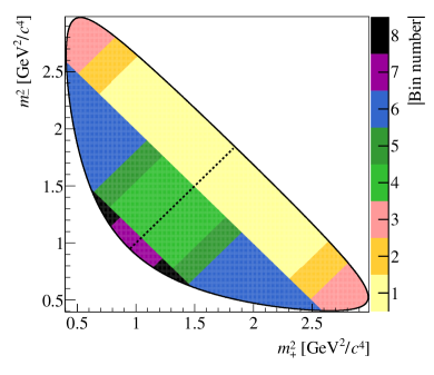
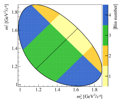
Figure 9: Rectangular binning schemes for (left) $D\rightarrow{{K}^{0}_{\mathrm{\scriptscriptstyle S}}}{{\pi}^{+}}{{\pi}^{-}}$ decays and (right) $D\rightarrow{{K}^{0}_{\mathrm{\scriptscriptstyle S}}}{{K}^{+}}{{K}^{-}}$ decays. The diagonal line separates the positive and negative bins, where the positive bins are in the region in which $m^{2}_{-}>m^{2}_{+}$ is satisfied.

Various effects are considered to assign an uncertainty for the imperfections in the description of the invariant-mass spectrum. For the PDF used to fit the signal, the parameters of the PDF used in the binned fit are varied according to the uncertainties obtained in the global fit. An alternative shape is also tested. The global fit is repeated with the mean and width of the shape used to describe the background due to misidentified companions allowed to vary freely. The results are used to generate data sets with an alternative PDF, and fit them using the default setup. The description of the partially reconstructed background is changed to a shape obtained from a fit of the PDF to simulated decays. The slope of the exponential used to fit the combinatorial background is also fluctuated according to the uncertainty obtained in the global fit. The contributions from each change are summed in quadrature and are $0.2\times 10^{-2}$ for each of the $x_{\pm}$ parameters and $0.3\times 10^{-2}$ for each of the $y_{\pm}$ parameters.

Two systematic uncertainties associated with the misidentified ${{B}^{\pm}}\rightarrow D{{\pi}^{\pm}}$ background in the ${{B}^{\pm}}\rightarrow D{{K}^{\pm}}$ sample are considered. First, the uncertainties on the particle misidentification probabilities are found to have a negligible effect on the measured values of $x_{\pm}$ and $y_{\pm}$. Second, it is possible that the invariant-mass distribution of the misidentified background (the mis-ID shape) is not uniform over the Dalitz plot, as assumed in the fit. This can occur through kinematic correlations between the reconstruction efficiency across the Dalitz plot of the $D$ decay and the momentum of the companion pion from the ${B}^{\pm}$ decay. Alternative mass shapes are constructed by repeating the procedure used to obtain the default shape for each Dalitz bin individually. The alternative shapes are used when generating data sets for pseudoexperiments, and the fits then performed assuming a single shape, as in the fit to data. The resulting uncertainty is at most $0.2\times 10^{-2}$ for all $C\!P$ parameters.

In the fit to the data, the relative contributions of the partially reconstructed ${B}^{\pm}$ and ${B}^{0}$ backgrounds are kept the same in each Dalitz bin. This is a simplification as some partially reconstructed backgrounds will be distributed as ${{D}^{0}}({{\kern 1.99997pt\overline{\kern-1.99997ptD}{}}{}^{0}})\rightarrow{{K}^{0}_{\mathrm{\scriptscriptstyle S}}}h^{+}h^{-}$ for reconstructed ${{B}^{-}}$ (${{B}^{+}}$) candidates, while partially reconstructed ${B}^{\pm}\rightarrow D^{(*)}K^{(*)\pm}$ decays will be distributed as a ${{D}^{0}}-{{\kern 1.99997pt\overline{\kern-1.99997ptD}{}}{}^{0}}$ admixture depending on the relevant $C\!P$ violation parameters. Pseudoexperiments are generated, where the $D$-decay Dalitz plot distribution for ${B}^{\pm}\rightarrow D^{*}K^{+}$ is based on the $C\!P$ parameters reported in Ref. [54] and those for ${B}^{\pm}\rightarrow DK^{*+}$ are taken from Ref. [55]. The generated samples are fitted with the standard method. The resulting uncertainty is at most $0.2\times 10^{-2}$ for all $C\!P$ parameters.

The total yield of the ${{B}^{0}_{s}}\rightarrow{{\kern 1.99997pt\overline{\kern-1.99997ptD}{}}{}^{0}}{{\pi}^{+}}{{K}^{-}}$ background in the ${{B}^{\pm}}\rightarrow D{{K}^{\pm}}$ channels is fixed relative to the corresponding ${{B}^{\pm}}\rightarrow D{{\pi}^{\pm}}$ yield. The systematic uncertainty due to the uncertainty on the relative rate is estimated via pseudoexperiments, where data sets are generated with the rate varied by $\pm 1\sigma$ and fitted using the default value. The maximal mean bias for each parameter is taken as the uncertainty. The resulting uncertainty is $0.1\times 10^{-2}$ for all $C\!P$ parameters.

An uncertainty is assigned to each $C\!P$ parameter to accompany the correction that is applied for the small bias observed in the fit procedure. These uncertainties are determined by performing sets of pseudoexperiments, each generated with different values of $x_{\pm}$ and $y_{\pm}$ throughout a range around the values predicted by the world averages. The spread in observed bias is combined in quadrature with the uncertainty in the precision of the pseudoexperiments. This is taken as the systematic uncertainty and is $0.1\times 10^{-2}$ for all $C\!P$ parameters.

The systematic uncertainty from the effect of candidates being assigned the wrong Dalitz bin number is considered. The resolution in $m^{2}_{+}$ and $m^{2}_{-}$ is approximately 0.006${\mathrm{\,Ge\kern-1.00006ptV^{2}\!/}c^{4}}$ for candidates with long ${K}^{0}_{\mathrm{\scriptscriptstyle S}}$ decays and 0.007${\mathrm{\,Ge\kern-1.00006ptV^{2}\!/}c^{4}}$ for candidates with downstream ${K}^{0}_{\mathrm{\scriptscriptstyle S}}$ decays. While this is small compared to the typical width of a bin, net migration can occur in regions where the presence of resonances cause the density to change rapidly. To first order this effect is accounted for by use of the control channel. However, differences in the distributions of the Dalitz plots due to efficiency differences or the nonzero value of $r_{B}$ in the signal decay may cause residual effects. The uncertainty from this is determined via pseudoexperiments, in which different input $F_{i}$ values are used to reflect the residual migration. The size of any possible bias is found to be $0.1\times 10^{-2}$ for all $C\!P$ parameters.

There is a systematic uncertainty related to $C\!P$ violation in the neutral kaon system due to the fact that the ${{K}^{0}_{\mathrm{\scriptscriptstyle S}}}$ state is not an exact $C\!P$ eigenstate and, separately, due to different nuclear interaction cross-sections of the ${K}^{0}$ and ${\kern 1.99997pt\overline{\kern-1.99997ptK}{}}{}^{0}$ mesons. The measurement is insensitive to global asymmetries, but is affected by the different Dalitz distributions of ${D}\rightarrow{{K}^{0}_{\mathrm{\scriptscriptstyle S}}}h^{-}h^{+}$ and ${D}\rightarrow{{K}^{0}_{\mathrm{\scriptscriptstyle L}}}h^{-}h^{+}$ decays, as well as any correlations between Dalitz coordinates and the net material interaction. The potential bias on $x_{\pm}$ and $y_{\pm}$ is assessed using a series of pseudoexperiments, where data are generated taking the effects into account and fitted using the default fit. The ${D}\rightarrow{{K}^{0}_{\mathrm{\scriptscriptstyle L}}}h^{-}h^{+}$ Dalitz distribution is estimated by transforming an amplitude model of ${D}\rightarrow{{K}^{0}_{\mathrm{\scriptscriptstyle S}}}h^{-}h^{+}$ [22], following arguments and assumptions laid out in Ref. [18]. The effect of material interaction is treated using the formalism described in Ref. [56]. The size of the potential bias is found to be $\leq 0.2\times 10^{-2}$ for all $C\!P$ parameters, corresponding to a bias on $\gamma$ of approximately $0.8^{\circ}$, which is within expected limits [57].

The nonuniform efficiency profile over the Dalitz plot means that the values of $(c_{i},s_{i})$ appropriate for this analysis can differ from those measured by the CLEO collaboration, which correspond to the constant-efficiency case. Amplitude models are used to calculate the values of $c_{i}$ and $s_{i}$ both with and without the efficiency profiles determined from simulation. The models are taken from Ref. [23] for $D\rightarrow{{K}^{0}_{\mathrm{\scriptscriptstyle S}}}{{\pi}^{+}}{{\pi}^{-}}$ decays and from Ref. [24] for $D\rightarrow{{K}^{0}_{\mathrm{\scriptscriptstyle S}}}{{K}^{+}}{{K}^{-}}$ decays. The difference is taken as an estimate of the size of this effect. Pseudoexperiments are generated in which the values have been shifted by this difference, and then fitted with the default $(c_{i},s_{i})$ values. The resulting bias on $x_{\pm}$ and $y_{\pm}$ is found to be negligible.

The effect that a detection asymmetry between hadrons of opposite charge can have on the symmetry of the efficiency across the Dalitz plot is found to be negligible. Changes in the mass model used to describe the semileptonic control sample are also found to have a negligible effect on the $F_{i}$ values.

Finally, several checks are conducted to assess the stability of the results. These include repeating the fits separately for both ${K}^{0}_{\mathrm{\scriptscriptstyle S}}$ categories, for each data-taking year, and by splitting the candidates depending on whether the hardware trigger decision was due to particles in the signal-candidate decay chain or other particles produced in the $pp$ collision. No anomalies are found and no additional systematic uncertainties are assigned.

In total the systematic uncertainties are less than half of the corresponding statistical uncertainties. The correlation matrix obtained for the combined effect of the sources of experimental and strong-phase related systematic uncertainties is given in Table 4.

Table 4: Correlation matrix of the experimental and strong-phase related systematic uncertainties.

	$\phantom{-}x_{-}$	$\phantom{-}y_{-}$	$\phantom{-}x_{+}$	$\phantom{-}y_{+}$
$x_{-}$	$\phantom{-}1$	$-0.25$	$\phantom{-}0.43$	$-0.09$
$y_{-}$		$\phantom{-}1$	$-0.20$	$-0.05$
$x_{+}$			$\phantom{-}1$	$\phantom{-}0.14$
$y_{+}$				$\phantom{-}1$

8 Results and interpretation

The $C\!P$ observables are measured to be

$$x_{-} =(\phantom{-}9.0\pm 1.7\pm 0.7\pm 0.4)\times 10^{-2},$$

$$y_{-} =(\phantom{-}2.1\pm 2.2\pm 0.5\pm 1.1)\times 10^{-2},$$

$$x_{+} =(-7.7\pm 1.9\pm 0.7\pm 0.4)\times 10^{-2},$$

$$y_{+} =(-1.0\pm 1.9\pm 0.4\pm 0.9)\times 10^{-2},$$

where the first uncertainty is statistical, the second is the total experimental systematic uncertainty and the third is that arising from the precision of the CLEO measurements.

The signature for $C\!P$ violation is that $(x_{+},y_{+})\neq(x_{-},y_{-})$. The distance between $(x_{+},y_{+})$ and $(x_{-},y_{-})$ is calculated, taking all uncertainties and correlations into account, and found to be $|(x_{+},y_{+})-(x_{-},y_{-})|=(17.0\pm 2.7)\times 10^{-2}$, which is different from zero by 6.4 standard deviations. This constitutes the first observation of $C\!P$ violation in ${{B}^{\pm}}\rightarrow D{{K}^{\pm}}$ decays for the ${D}\rightarrow{{K}^{0}_{\mathrm{\scriptscriptstyle S}}}h^{+}h^{-}$ final states.

These results are compared to the expected central values of $x_{\pm}$ and $y_{\pm}$ that can be computed from $r_{B},\delta_{B}$, and $\gamma$ as determined in the LHCb combination in Ref. [54], and the results are shown in Fig. 10 (the later LHCb combination in Ref. [58] includes the results of this measurement and is therefore unsuitable for comparison). The two sets of $(x_{+},y_{+})$ are in agreement within 1.6 standard deviations when the uncertainties and correlations of both the LHCb combination and this measurement are taken into account. There is a 2.7 standard deviation tension between the measured values of $(x_{-},\,y_{-})$ and the values calculated from the LHCb combination. This tension will be investigated further when this measurement and the LHCb combination are updated using data taken in 2017 and 2018.

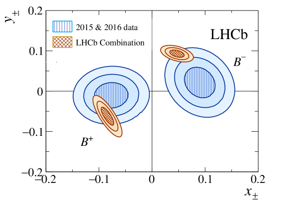
Figure 10: Two-dimensional 68.3 %, 95.5 % and 99.7 % confidence regions for $(x_{\pm},\,y_{\pm})$ obtained in this measurement, as well as for the LHCb combination in Ref. [54], taking statistical and systematic uncertainties, as well as their correlations, into account.

The results for $x_{\pm}$ and $y_{\pm}$ are interpreted in terms of the underlying physics parameters $\gamma$, $r_{B}$ and $\delta_{B}$. The interpretation is done via a maximum likelihood fit using a frequentist treatment as described in Ref. [59]. The solution for the physics parameters has a two-fold ambiguity as the equations are invariant under the simultaneous substitutions $\gamma\rightarrow\gamma+180^{\circ}$ and $\delta_{B}\rightarrow\delta_{B}+180^{\circ}$. The solution that satisfies $0<\gamma<180^{\circ}$ is chosen. The central values and 68% (95%) confidence intervals, calculated with the PLUGIN [60] method, are

$$\gamma =87^{\circ}\,{}^{+11^{\circ}}_{-12^{\circ}}\left({}^{+22^{\circ}}_{-23^{\circ}}\right),$$

$$r_{B} =0.086\,^{+0.013}_{-0.014}\left({}^{+0.025}_{-0.027}\right),$$

$$\delta_{B} =101^{\circ}\,{}^{+11^{\circ}}_{-11^{\circ}}\left({}^{+22^{\circ}}_{-23^{\circ}}\right).$$

The values for $\gamma$ and $r_{B}$ are consistent with those presented in Ref. [54]. This is the most precise measurement of $\gamma$ from a single analysis. The value of $\delta_{B}$ shows some disagreement with Ref. [54], where the angle is determined to be $\left(139.9\,^{+4.8}_{-5.2}\right)^{\circ}$.

The values of $x_{\pm},y_{\pm}$ measured in this analysis can be combined with those from the corresponding analysis of Run 1 data [9]. This procedure is done via a maximum likelihood fit, as implemented in the gammacombo package [59]. The previous measurements are identified by the index I, and the results within this paper are identified by the index II. When combining the two results, the fit determines the $(\hat{x}_{\pm},\hat{y}_{\pm})$ parameters that maximize the multivariate Gaussian likelihood function

$$\mathcal{L}(z|\hat{z})=((2\pi)^{8}|\Sigma|)^{-1/2}\exp\left[-\frac{1}{2}(z-\hat{z})^{T}\Sigma^{-1}(z-\hat{z})\right],$$ (16)

where $z=(x_{\pm}^{\text{I}},y_{\pm}^{\text{I}},x_{\pm}^{\text{II}},y_{\pm}^{\text{II}})^{T}$ and $\hat{z}=(\hat{x}_{\pm},\hat{y}_{\pm},\hat{x}_{\pm},\hat{y}_{\pm})^{T}$ are $8\times 1$ vectors and $\Sigma$ is the $8\times 8$ covariance matrix

$$\Sigma=\left(\begin{array}[]{cc}\Sigma^{\text{I}}&\Sigma^{\text{I--II}}\\ \Sigma^{\text{II--I}}&\Sigma^{\text{II}}\end{array}\right).$$ (19)

The covariance matrix is expressed in terms of the covariance matrices obtained for the individual measurements, $\Sigma^{\text{I}}$ and $\Sigma^{\text{II}}$, and the cross-covariance matrix $\Sigma^{\text{I--II}}$ describing correlations between the measurements. The covariance matrix for this measurement, $\Sigma^{\text{II}}$, is calculated using the total statistical and systematic uncertainties, and the correlation matrices in Tables 1 and 4. The covariance matrix for the Run 1 measurement, $\Sigma^{\text{I}}$, is taken from Ref. [9], where it was calculated taking strong-phase-related correlations into account, but treating the experimental systematic uncertainties as uncorrelated. The impact of using the correlation matrix in Table 4 for these instead is found to be negligible.

The dominant uncertainty in both measurements is the statistical uncertainty. As the measurements use independent data sets, the statistical uncertainties are uncorrelated. The cross-correlations of the systematic errors between measurements due to the strong phase inputs are obtained from the results of a series of fits to the two data sets in which the strong phases are varied identically. This mirrors the procedure used to evaluate the uncertainties within a single data set. The obtained cross-correlations between the fit results are given in Table 5. The elements on the diagonal do not have unit value because the obtained correlations depend on the specific data sets for the two measurements.

Table 5: Correlation matrix between Run 1 results (I) and the results presented in this paper (II), when fitting data while varying the inputs from the CLEO collaboration in a correlated way.

CLEO cross-run correlation matrix
	$\phantom{-}x_{-}^{\text{II}}$	$\phantom{-}y_{-}^{\text{II}}$	$\phantom{-}x_{+}^{\text{II}}$	$\phantom{-}y_{+}^{\text{II}}$
$x_{-}^{\text{I}}$	$\phantom{-}0.02$	$\phantom{-}0.35$	$-0.32$	$-0.21$
$y_{-}^{\text{I}}$	$\phantom{-}0.45$	$-0.23$	$\phantom{-}0.03$	$-0.28$
$x_{+}^{\text{I}}$	$-0.19$	$\phantom{-}0.01$	$\phantom{-}0.55$	$-0.22$
$y_{+}^{\text{I}}$	$-0.30$	$-0.28$	$\phantom{-}0.13$	$\phantom{-}0.48$

Table 6: Total correlation matrix for the systematic uncertainties of the Run 1 results (I) and the results presented in this paper (II), including experimental and strong phase related systematic uncertainties.

Total systematic cross-run correlation matrix
	$\phantom{-}x_{-}^{\text{II}}$	$\phantom{-}y_{-}^{\text{II}}$	$\phantom{-}x_{+}^{\text{II}}$	$\phantom{-}y_{+}^{\text{II}}$
$x_{-}^{\text{I}}$	$\phantom{-}0.76$	$\phantom{-}0.04$	$\phantom{-}0.55$	$\phantom{-}0.02$
$y_{-}^{\text{I}}$	$\phantom{-}0.14$	$-0.06$	$-0.13$	$-0.25$
$x_{+}^{\text{I}}$	$\phantom{-}0.58$	$-0.19$	$\phantom{-}0.91$	$\phantom{-}0.05$
$y_{+}^{\text{I}}$	$-0.05$	$-0.24$	$\phantom{-}0.17$	$\phantom{-}0.55$

The combination is performed assuming full correlation between the non-strong-phase related experimental systematic uncertainties in Run 1 and this measurement. The correlation matrix for the experimental uncertainties of this analysis is used as the cross-run correlation of the experimental systematic uncertainties. The complete correlation matrix for the experimental and strong-phase-related systematic uncertainties is given in Table 6. The impact on the combination due to different assumptions on the cross-correlations of the systematic uncertainties is found to be negligible. This is unsurprising as both measurements remain limited in precision by their statistical uncertainties. The central values, along with the combined statistical and systematic uncertainties for this combination are

$$<x_{-}> =(\phantom{-}7.0\pm 1.7)\times 10^{-2},$$

$$<y_{-}> =(\phantom{-}4.1\pm 2.0)\times 10^{-2},$$

$$<x_{+}> =(-7.8\pm 1.7)\times 10^{-2},$$

$$<y_{+}> =(-1.4\pm 1.7)\times 10^{-2}.$$

The interpretation in terms of the underlying physics parameters is performed on the combined values of $x_{\pm}$ and $y_{\pm}$ and the central values and their 68$\%$ (95$\%$) confidence intervals are

$$\gamma =80^{\circ}\,{}^{+10^{\circ}}_{-9^{\circ}}\left({}^{+19^{\circ}}_{-18^{\circ}}\right),$$

$$r_{B} =0.080\,^{+0.011}_{-0.011}\left({}^{+0.022}_{-0.023}\right),$$

$$\delta_{B} =110^{\circ}\,{}^{+10^{\circ}}_{-10^{\circ}}\left({}^{+19^{\circ}}_{-20^{\circ}}\right).$$

The results of the interpretation for both the combined and individual data sets are shown in Fig. 11, where the projections of the three-dimensional surfaces bounding the one and two standard deviation volumes on the ($\gamma$, $r_{B}$) and ($\gamma$, $\delta_{B}$) planes are shown. The uncertainty on $\gamma$ is inversely proportional to $r_{B}$. Therefore the lower central value of $r_{B}$ in the combined results lead to a larger than naively expected uncertainty on $\gamma$ when both data sets are used. The contribution of each source of uncertainty are estimated by performing the combination while taking only subsets of the uncertainties into account. It is found that the statistical uncertainty on $\gamma$ is $8.5^{\circ}$, the uncertainty due to strong-phase inputs is $4^{\circ}$, and the uncertainty due to experimental systematic effects is $2^{\circ}$.

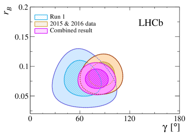
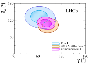
Figure 11: Two-dimensional 68.3 % and 95.5 % confidence regions for $(\gamma,r_{B},\delta_{B})$ for the $x_{\pm}$, $y_{\pm}$ parameters obtained in the fit to 2015 and 2016 data, the fit to Run 1 data, and their combinations.

9 Conclusions

Approximately 4100 (560) $B^{\pm}\rightarrow DK^{\pm}$ decays with the $D$ meson decaying to ${{K}^{0}_{\mathrm{\scriptscriptstyle S}}}\pi^{+}\pi^{-}$ (${{K}^{0}_{\mathrm{\scriptscriptstyle S}}}K^{+}K^{-}$) are selected from data corresponding to an integrated luminosity of 2.0 ${\rm fb^{-1}}$ collected with the LHCb detector in 2015 and 2016. These samples are analysed to determine the $C\!P$-violating parameters $x_{\pm}\equiv r_{B}\cos(\delta_{B}\pm\gamma)$ and $y_{\pm}\equiv r_{B}\sin(\delta_{B}\pm\gamma)$, where $r_{B}$ is the ratio of the absolute values of the $B^{+}\rightarrow D^{0}K^{-}$ and $B^{+}\rightarrow{{\kern 1.99997pt\overline{\kern-1.99997ptD}{}}{}^{0}}K^{-}$ amplitudes, $\delta_{B}$ is their strong-phase differences, and $\gamma$ is an angle of the Unitarity Triangle. The analysis is performed in bins of the $D$-decay Dalitz plot and existing measurements performed by the CLEO collaboration [18] are used to provide input on the $D$-decay strong-phase parameters $(c_{i},s_{i})$. Such an approach allows the analysis to be free from model-dependent assumptions on the strong-phase variation across the Dalitz plot. This paper also gives the combination with the results obtained with an earlier data set, thereby allowing further improvements in the precision on $\gamma$. Considering only the data collected in 2015 and 2016 and choosing the solution that satisfies $0<\gamma<180^{\circ}$ yields $r_{B}$ = $0.086^{+0.013}_{-0.014}$, $\delta_{B}=(101\pm 11)^{\circ}$, and $\gamma=(87^{+11}_{-12})^{\circ}$. The values of $r_{B}$ and $\gamma$ are consistent with world averages, while there is some tension in the determined value of $\delta_{B}$. This could be resolved by future analyses of the $B\rightarrow DK$ mode in a variety of $D$ decays, including those analysed here, utilising the data set that is being collected with LHCb in 2017 and 2018. The measurement reported in this paper represents the most precise determination of $\gamma$ from a single analysis.

LHCb collaboration

R. Aaij²⁷, B. Adeva⁴¹, M. Adinolfi⁴⁸, C.A. Aidala⁷³, Z. Ajaltouni⁵, S. Akar⁵⁹, P. Albicocco¹⁸, J. Albrecht¹⁰, F. Alessio⁴², M. Alexander⁵³, A. Alfonso Albero⁴⁰, S. Ali²⁷, G. Alkhazov³³, P. Alvarez Cartelle⁵⁵, A.A. Alves Jr⁵⁹, S. Amato², S. Amerio²³, Y. Amhis⁷, L. An³, L. Anderlini¹⁷, G. Andreassi⁴³, M. Andreotti^16,g, J.E. Andrews⁶⁰, R.B. Appleby⁵⁶, F. Archilli²⁷, P. d’Argent¹², J. Arnau Romeu⁶, A. Artamonov³⁹, M. Artuso⁶¹, K. Arzymatov³⁷, E. Aslanides⁶, M. Atzeni⁴⁴, S. Bachmann¹², J.J. Back⁵⁰, S. Baker⁵⁵, V. Balagura^7,b, W. Baldini¹⁶, A. Baranov³⁷, R.J. Barlow⁵⁶, S. Barsuk⁷, W. Barter⁵⁶, F. Baryshnikov⁷⁰, V. Batozskaya³¹, B. Batsukh⁶¹, V. Battista⁴³, A. Bay⁴³, J. Beddow⁵³, F. Bedeschi²⁴, I. Bediaga¹, A. Beiter⁶¹, L.J. Bel²⁷, N. Beliy⁶³, V. Bellee⁴³, N. Belloli^20,i, K. Belous³⁹, I. Belyaev^34,42, E. Ben-Haim⁸, G. Bencivenni¹⁸, S. Benson²⁷, S. Beranek⁹, A. Berezhnoy³⁵, R. Bernet⁴⁴, D. Berninghoff¹², E. Bertholet⁸, A. Bertolin²³, C. Betancourt⁴⁴, F. Betti^15,42, M.O. Bettler⁴⁹, M. van Beuzekom²⁷, Ia. Bezshyiko⁴⁴, S. Bhasin⁴⁸, J. Bhom²⁹, S. Bifani⁴⁷, P. Billoir⁸, A. Birnkraut¹⁰, A. Bizzeti^17,u, M. Bjørn⁵⁷, M.P. Blago⁴², T. Blake⁵⁰, F. Blanc⁴³, S. Blusk⁶¹, D. Bobulska⁵³, V. Bocci²⁶, O. Boente Garcia⁴¹, T. Boettcher⁵⁸, A. Bondar^38,w, N. Bondar³³, S. Borghi^56,42, M. Borisyak³⁷, M. Borsato^41,42, F. Bossu⁷, M. Boubdir⁹, T.J.V. Bowcock⁵⁴, C. Bozzi^16,42, S. Braun¹², M. Brodski⁴², J. Brodzicka²⁹, D. Brundu²², E. Buchanan⁴⁸, A. Buonaura⁴⁴, C. Burr⁵⁶, A. Bursche²², J. Buytaert⁴², W. Byczynski⁴², S. Cadeddu²², H. Cai⁶⁴, R. Calabrese^16,g, R. Calladine⁴⁷, M. Calvi^20,i, M. Calvo Gomez^40,m, A. Camboni^40,m, P. Campana¹⁸, D.H. Campora Perez⁴², L. Capriotti⁵⁶, A. Carbone^15,e, G. Carboni²⁵, R. Cardinale^19,h, A. Cardini²², P. Carniti^20,i, L. Carson⁵², K. Carvalho Akiba², G. Casse⁵⁴, L. Cassina²⁰, M. Cattaneo⁴², G. Cavallero^19,h, R. Cenci^24,p, D. Chamont⁷, M.G. Chapman⁴⁸, M. Charles⁸, Ph. Charpentier⁴², G. Chatzikonstantinidis⁴⁷, M. Chefdeville⁴, V. Chekalina³⁷, C. Chen³, S. Chen²², S.-G. Chitic⁴², V. Chobanova⁴¹, M. Chrzaszcz⁴², A. Chubykin³³, P. Ciambrone¹⁸, X. Cid Vidal⁴¹, G. Ciezarek⁴², P.E.L. Clarke⁵², M. Clemencic⁴², H.V. Cliff⁴⁹, J. Closier⁴², V. Coco⁴², J. Cogan⁶, E. Cogneras⁵, L. Cojocariu³², P. Collins⁴², T. Colombo⁴², A. Comerma-Montells¹², A. Contu²², G. Coombs⁴², S. Coquereau⁴⁰, G. Corti⁴², M. Corvo^16,g, C.M. Costa Sobral⁵⁰, B. Couturier⁴², G.A. Cowan⁵², D.C. Craik⁵⁸, A. Crocombe⁵⁰, M. Cruz Torres¹, R. Currie⁵², C. D’Ambrosio⁴², F. Da Cunha Marinho², C.L. Da Silva⁷⁴, E. Dall’Occo²⁷, J. Dalseno⁴⁸, A. Danilina³⁴, A. Davis³, O. De Aguiar Francisco⁴², K. De Bruyn⁴², S. De Capua⁵⁶, M. De Cian⁴³, J.M. De Miranda¹, L. De Paula², M. De Serio^14,d, P. De Simone¹⁸, C.T. Dean⁵³, D. Decamp⁴, L. Del Buono⁸, B. Delaney⁴⁹, H.-P. Dembinski¹¹, M. Demmer¹⁰, A. Dendek³⁰, D. Derkach³⁷, O. Deschamps⁵, F. Desse⁷, F. Dettori⁵⁴, B. Dey⁶⁵, A. Di Canto⁴², P. Di Nezza¹⁸, S. Didenko⁷⁰, H. Dijkstra⁴², F. Dordei⁴², M. Dorigo^42,y, A. Dosil Suárez⁴¹, L. Douglas⁵³, A. Dovbnya⁴⁵, K. Dreimanis⁵⁴, L. Dufour²⁷, G. Dujany⁸, P. Durante⁴², J.M. Durham⁷⁴, D. Dutta⁵⁶, R. Dzhelyadin³⁹, M. Dziewiecki¹², A. Dziurda²⁹, A. Dzyuba³³, S. Easo⁵¹, U. Egede⁵⁵, V. Egorychev³⁴, S. Eidelman^38,w, S. Eisenhardt⁵², U. Eitschberger¹⁰, R. Ekelhof¹⁰, L. Eklund⁵³, S. Ely⁶¹, A. Ene³², S. Escher⁹, S. Esen²⁷, T. Evans⁵⁹, A. Falabella¹⁵, N. Farley⁴⁷, S. Farry⁵⁴, D. Fazzini^20,42,i, L. Federici²⁵, G. Fernandez⁴⁰, P. Fernandez Declara⁴², A. Fernandez Prieto⁴¹, F. Ferrari¹⁵, L. Ferreira Lopes⁴³, F. Ferreira Rodrigues², M. Ferro-Luzzi⁴², S. Filippov³⁶, R.A. Fini¹⁴, M. Fiorini^16,g, M. Firlej³⁰, C. Fitzpatrick⁴³, T. Fiutowski³⁰, F. Fleuret^7,b, M. Fontana^22,42, F. Fontanelli^19,h, R. Forty⁴², V. Franco Lima⁵⁴, M. Frank⁴², C. Frei⁴², J. Fu^21,q, W. Funk⁴², C. Färber⁴², M. Féo Pereira Rivello Carvalho²⁷, E. Gabriel⁵², A. Gallas Torreira⁴¹, D. Galli^15,e, S. Gallorini²³, S. Gambetta⁵², M. Gandelman², P. Gandini²¹, Y. Gao³, L.M. Garcia Martin⁷², B. Garcia Plana⁴¹, J. García Pardiñas⁴⁴, J. Garra Tico⁴⁹, L. Garrido⁴⁰, D. Gascon⁴⁰, C. Gaspar⁴², L. Gavardi¹⁰, G. Gazzoni⁵, D. Gerick¹², E. Gersabeck⁵⁶, M. Gersabeck⁵⁶, T. Gershon⁵⁰, D. Gerstel⁶, Ph. Ghez⁴, S. Gianì⁴³, V. Gibson⁴⁹, O.G. Girard⁴³, L. Giubega³², K. Gizdov⁵², V.V. Gligorov⁸, D. Golubkov³⁴, A. Golutvin^55,70, A. Gomes^1,a, I.V. Gorelov³⁵, C. Gotti^20,i, E. Govorkova²⁷, J.P. Grabowski¹², R. Graciani Diaz⁴⁰, L.A. Granado Cardoso⁴², E. Graugés⁴⁰, E. Graverini⁴⁴, G. Graziani¹⁷, A. Grecu³², R. Greim²⁷, P. Griffith²², L. Grillo⁵⁶, L. Gruber⁴², B.R. Gruberg Cazon⁵⁷, O. Grünberg⁶⁷, C. Gu³, E. Gushchin³⁶, Yu. Guz^39,42, T. Gys⁴², C. Göbel⁶², T. Hadavizadeh⁵⁷, C. Hadjivasiliou⁵, G. Haefeli⁴³, C. Haen⁴², S.C. Haines⁴⁹, B. Hamilton⁶⁰, X. Han¹², T.H. Hancock⁵⁷, S. Hansmann-Menzemer¹², N. Harnew⁵⁷, S.T. Harnew⁴⁸, T. Harrison⁵⁴, C. Hasse⁴², M. Hatch⁴², J. He⁶³, M. Hecker⁵⁵, K. Heinicke¹⁰, A. Heister⁹, K. Hennessy⁵⁴, L. Henry⁷², E. van Herwijnen⁴², M. Heß⁶⁷, A. Hicheur², D. Hill⁵⁷, M. Hilton⁵⁶, P.H. Hopchev⁴³, W. Hu⁶⁵, W. Huang⁶³, Z.C. Huard⁵⁹, W. Hulsbergen²⁷, T. Humair⁵⁵, M. Hushchyn³⁷, D. Hutchcroft⁵⁴, D. Hynds²⁷, P. Ibis¹⁰, M. Idzik³⁰, P. Ilten⁴⁷, K. Ivshin³³, R. Jacobsson⁴², J. Jalocha⁵⁷, E. Jans²⁷, A. Jawahery⁶⁰, F. Jiang³, M. John⁵⁷, D. Johnson⁴², C.R. Jones⁴⁹, C. Joram⁴², B. Jost⁴², N. Jurik⁵⁷, S. Kandybei⁴⁵, M. Karacson⁴², J.M. Kariuki⁴⁸, S. Karodia⁵³, N. Kazeev³⁷, M. Kecke¹², F. Keizer⁴⁹, M. Kelsey⁶¹, M. Kenzie⁴⁹, T. Ketel²⁸, E. Khairullin³⁷, B. Khanji¹², C. Khurewathanakul⁴³, K.E. Kim⁶¹, T. Kirn⁹, S. Klaver¹⁸, K. Klimaszewski³¹, T. Klimkovich¹¹, S. Koliiev⁴⁶, M. Kolpin¹², R. Kopecna¹², P. Koppenburg²⁷, I. Kostiuk²⁷, S. Kotriakhova³³, M. Kozeiha⁵, L. Kravchuk³⁶, M. Kreps⁵⁰, F. Kress⁵⁵, P. Krokovny^38,w, W. Krupa³⁰, W. Krzemien³¹, W. Kucewicz^29,l, M. Kucharczyk²⁹, V. Kudryavtsev^38,w, A.K. Kuonen⁴³, T. Kvaratskheliya^34,42, D. Lacarrere⁴², G. Lafferty⁵⁶, A. Lai²², D. Lancierini⁴⁴, G. Lanfranchi¹⁸, C. Langenbruch⁹, T. Latham⁵⁰, C. Lazzeroni⁴⁷, R. Le Gac⁶, A. Leflat³⁵, J. Lefrançois⁷, R. Lefèvre⁵, F. Lemaitre⁴², O. Leroy⁶, T. Lesiak²⁹, B. Leverington¹², P.-R. Li⁶³, T. Li³, Z. Li⁶¹, X. Liang⁶¹, T. Likhomanenko⁶⁹, R. Lindner⁴², F. Lionetto⁴⁴, V. Lisovskyi⁷, X. Liu³, D. Loh⁵⁰, A. Loi²², I. Longstaff⁵³, J.H. Lopes², G.H. Lovell⁴⁹, D. Lucchesi^23,o, M. Lucio Martinez⁴¹, A. Lupato²³, E. Luppi^16,g, O. Lupton⁴², A. Lusiani²⁴, X. Lyu⁶³, F. Machefert⁷, F. Maciuc³², V. Macko⁴³, P. Mackowiak¹⁰, S. Maddrell-Mander⁴⁸, O. Maev^33,42, K. Maguire⁵⁶, D. Maisuzenko³³, M.W. Majewski³⁰, S. Malde⁵⁷, B. Malecki²⁹, A. Malinin⁶⁹, T. Maltsev^38,w, G. Manca^22,f, G. Mancinelli⁶, D. Marangotto^21,q, J. Maratas^5,v, J.F. Marchand⁴, U. Marconi¹⁵, C. Marin Benito⁴⁰, M. Marinangeli⁴³, P. Marino⁴³, J. Marks¹², G. Martellotti²⁶, M. Martin⁶, M. Martinelli⁴², D. Martinez Santos⁴¹, F. Martinez Vidal⁷², A. Massafferri¹, R. Matev⁴², A. Mathad⁵⁰, Z. Mathe⁴², C. Matteuzzi²⁰, A. Mauri⁴⁴, E. Maurice^7,b, B. Maurin⁴³, A. Mazurov⁴⁷, M. McCann^55,42, A. McNab⁵⁶, R. McNulty¹³, J.V. Mead⁵⁴, B. Meadows⁵⁹, C. Meaux⁶, F. Meier¹⁰, N. Meinert⁶⁷, D. Melnychuk³¹, M. Merk²⁷, A. Merli^21,q, E. Michielin²³, D.A. Milanes⁶⁶, E. Millard⁵⁰, M.-N. Minard⁴, L. Minzoni^16,g, D.S. Mitzel¹², A. Mogini⁸, J. Molina Rodriguez^1,z, T. Mombächer¹⁰, I.A. Monroy⁶⁶, S. Monteil⁵, M. Morandin²³, G. Morello¹⁸, M.J. Morello^24,t, O. Morgunova⁶⁹, J. Moron³⁰, A.B. Morris⁶, R. Mountain⁶¹, F. Muheim⁵², M. Mulder²⁷, C.H. Murphy⁵⁷, D. Murray⁵⁶, D. Müller⁴², J. Müller¹⁰, K. Müller⁴⁴, V. Müller¹⁰, P. Naik⁴⁸, T. Nakada⁴³, R. Nandakumar⁵¹, A. Nandi⁵⁷, T. Nanut⁴³, I. Nasteva², M. Needham⁵², N. Neri²¹, S. Neubert¹², N. Neufeld⁴², M. Neuner¹², T.D. Nguyen⁴³, C. Nguyen-Mau^43,n, S. Nieswand⁹, R. Niet¹⁰, N. Nikitin³⁵, A. Nogay⁶⁹, D.P. O’Hanlon¹⁵, A. Oblakowska-Mucha³⁰, V. Obraztsov³⁹, S. Ogilvy¹⁸, R. Oldeman^22,f, C.J.G. Onderwater⁶⁸, A. Ossowska²⁹, J.M. Otalora Goicochea², P. Owen⁴⁴, A. Oyanguren⁷², P.R. Pais⁴³, A. Palano¹⁴, M. Palutan^18,42, G. Panshin⁷¹, A. Papanestis⁵¹, M. Pappagallo⁵², L.L. Pappalardo^16,g, W. Parker⁶⁰, C. Parkes⁵⁶, G. Passaleva^17,42, A. Pastore¹⁴, M. Patel⁵⁵, C. Patrignani^15,e, A. Pearce⁴², A. Pellegrino²⁷, G. Penso²⁶, M. Pepe Altarelli⁴², S. Perazzini⁴², D. Pereima³⁴, P. Perret⁵, L. Pescatore⁴³, K. Petridis⁴⁸, A. Petrolini^19,h, A. Petrov⁶⁹, S. Petrucci⁵², M. Petruzzo^21,q, B. Pietrzyk⁴, G. Pietrzyk⁴³, M. Pikies²⁹, M. Pili⁵⁷, D. Pinci²⁶, J. Pinzino⁴², F. Pisani⁴², A. Piucci¹², V. Placinta³², S. Playfer⁵², J. Plews⁴⁷, M. Plo Casasus⁴¹, F. Polci⁸, M. Poli Lener¹⁸, A. Poluektov⁵⁰, N. Polukhina^70,c, I. Polyakov⁶¹, E. Polycarpo², G.J. Pomery⁴⁸, S. Ponce⁴², A. Popov³⁹, D. Popov^47,11, S. Poslavskii³⁹, C. Potterat², E. Price⁴⁸, J. Prisciandaro⁴¹, C. Prouve⁴⁸, V. Pugatch⁴⁶, A. Puig Navarro⁴⁴, H. Pullen⁵⁷, G. Punzi^24,p, W. Qian⁶³, J. Qin⁶³, R. Quagliani⁸, B. Quintana⁵, B. Rachwal³⁰, J.H. Rademacker⁴⁸, M. Rama²⁴, M. Ramos Pernas⁴¹, M.S. Rangel², F. Ratnikov^37,x, G. Raven²⁸, M. Ravonel Salzgeber⁴², M. Reboud⁴, F. Redi⁴³, S. Reichert¹⁰, A.C. dos Reis¹, F. Reiss⁸, C. Remon Alepuz⁷², Z. Ren³, V. Renaudin⁷, S. Ricciardi⁵¹, S. Richards⁴⁸, K. Rinnert⁵⁴, P. Robbe⁷, A. Robert⁸, A.B. Rodrigues⁴³, E. Rodrigues⁵⁹, J.A. Rodriguez Lopez⁶⁶, M. Roehrken⁴², A. Rogozhnikov³⁷, S. Roiser⁴², A. Rollings⁵⁷, V. Romanovskiy³⁹, A. Romero Vidal⁴¹, M. Rotondo¹⁸, M.S. Rudolph⁶¹, T. Ruf⁴², J. Ruiz Vidal⁷², J.J. Saborido Silva⁴¹, N. Sagidova³³, B. Saitta^22,f, V. Salustino Guimaraes⁶², C. Sanchez Gras²⁷, C. Sanchez Mayordomo⁷², B. Sanmartin Sedes⁴¹, R. Santacesaria²⁶, C. Santamarina Rios⁴¹, M. Santimaria¹⁸, E. Santovetti^25,j, G. Sarpis⁵⁶, A. Sarti^18,k, C. Satriano^26,s, A. Satta²⁵, M. Saur⁶³, D. Savrina^34,35, S. Schael⁹, M. Schellenberg¹⁰, M. Schiller⁵³, H. Schindler⁴², M. Schmelling¹¹, T. Schmelzer¹⁰, B. Schmidt⁴², O. Schneider⁴³, A. Schopper⁴², H.F. Schreiner⁵⁹, M. Schubiger⁴³, M.H. Schune⁷, R. Schwemmer⁴², B. Sciascia¹⁸, A. Sciubba^26,k, A. Semennikov³⁴, E.S. Sepulveda⁸, A. Sergi^47,42, N. Serra⁴⁴, J. Serrano⁶, L. Sestini²³, P. Seyfert⁴², M. Shapkin³⁹, Y. Shcheglov^33,†, T. Shears⁵⁴, L. Shekhtman^38,w, V. Shevchenko⁶⁹, E. Shmanin⁷⁰, B.G. Siddi¹⁶, R. Silva Coutinho⁴⁴, L. Silva de Oliveira², G. Simi^23,o, S. Simone^14,d, N. Skidmore¹², T. Skwarnicki⁶¹, J.G. Smeaton⁴⁹, E. Smith⁹, I.T. Smith⁵², M. Smith⁵⁵, M. Soares¹⁵, l. Soares Lavra¹, M.D. Sokoloff⁵⁹, F.J.P. Soler⁵³, B. Souza De Paula², B. Spaan¹⁰, P. Spradlin⁵³, F. Stagni⁴², M. Stahl¹², S. Stahl⁴², P. Stefko⁴³, S. Stefkova⁵⁵, O. Steinkamp⁴⁴, S. Stemmle¹², O. Stenyakin³⁹, M. Stepanova³³, H. Stevens¹⁰, S. Stone⁶¹, B. Storaci⁴⁴, S. Stracka^24,p, M.E. Stramaglia⁴³, M. Straticiuc³², U. Straumann⁴⁴, S. Strokov⁷¹, J. Sun³, L. Sun⁶⁴, K. Swientek³⁰, V. Syropoulos²⁸, T. Szumlak³⁰, M. Szymanski⁶³, S. T’Jampens⁴, Z. Tang³, A. Tayduganov⁶, T. Tekampe¹⁰, G. Tellarini¹⁶, F. Teubert⁴², E. Thomas⁴², J. van Tilburg²⁷, M.J. Tilley⁵⁵, V. Tisserand⁵, S. Tolk⁴², L. Tomassetti^16,g, D. Tonelli²⁴, D.Y. Tou⁸, R. Tourinho Jadallah Aoude¹, E. Tournefier⁴, M. Traill⁵³, M.T. Tran⁴³, A. Trisovic⁴⁹, A. Tsaregorodtsev⁶, A. Tully⁴⁹, N. Tuning^27,42, A. Ukleja³¹, A. Usachov⁷, A. Ustyuzhanin³⁷, U. Uwer¹², C. Vacca^22,f, A. Vagner⁷¹, V. Vagnoni¹⁵, A. Valassi⁴², S. Valat⁴², G. Valenti¹⁵, R. Vazquez Gomez⁴², P. Vazquez Regueiro⁴¹, S. Vecchi¹⁶, M. van Veghel²⁷, J.J. Velthuis⁴⁸, M. Veltri^17,r, G. Veneziano⁵⁷, A. Venkateswaran⁶¹, T.A. Verlage⁹, M. Vernet⁵, M. Vesterinen⁵⁷, J.V. Viana Barbosa⁴², D.  Vieira⁶³, M. Vieites Diaz⁴¹, H. Viemann⁶⁷, X. Vilasis-Cardona^40,m, A. Vitkovskiy²⁷, M. Vitti⁴⁹, V. Volkov³⁵, A. Vollhardt⁴⁴, B. Voneki⁴², A. Vorobyev³³, V. Vorobyev^38,w, J.A. de Vries²⁷, C. Vázquez Sierra²⁷, R. Waldi⁶⁷, J. Walsh²⁴, J. Wang⁶¹, M. Wang³, Y. Wang⁶⁵, Z. Wang⁴⁴, D.R. Ward⁴⁹, H.M. Wark⁵⁴, N.K. Watson⁴⁷, D. Websdale⁵⁵, A. Weiden⁴⁴, C. Weisser⁵⁸, M. Whitehead⁹, J. Wicht⁵⁰, G. Wilkinson⁵⁷, M. Wilkinson⁶¹, I. Williams⁴⁹, M.R.J. Williams⁵⁶, M. Williams⁵⁸, T. Williams⁴⁷, F.F. Wilson^51,42, J. Wimberley⁶⁰, M. Winn⁷, J. Wishahi¹⁰, W. Wislicki³¹, M. Witek²⁹, G. Wormser⁷, S.A. Wotton⁴⁹, K. Wyllie⁴², D. Xiao⁶⁵, Y. Xie⁶⁵, A. Xu³, M. Xu⁶⁵, Q. Xu⁶³, Z. Xu³, Z. Xu⁴, Z. Yang³, Z. Yang⁶⁰, Y. Yao⁶¹, L.E. Yeomans⁵⁴, H. Yin⁶⁵, J. Yu^65,ab, X. Yuan⁶¹, O. Yushchenko³⁹, K.A. Zarebski⁴⁷, M. Zavertyaev^11,c, D. Zhang⁶⁵, L. Zhang³, W.C. Zhang^3,aa, Y. Zhang⁷, A. Zhelezov¹², Y. Zheng⁶³, X. Zhu³, V. Zhukov^9,35, J.B. Zonneveld⁵², S. Zucchelli¹⁵.

¹Centro Brasileiro de Pesquisas Físicas (CBPF), Rio de Janeiro, Brazil
²Universidade Federal do Rio de Janeiro (UFRJ), Rio de Janeiro, Brazil
³Center for High Energy Physics, Tsinghua University, Beijing, China
⁴Univ. Grenoble Alpes, Univ. Savoie Mont Blanc, CNRS, IN2P3-LAPP, Annecy, France
⁵Clermont Université, Université Blaise Pascal, CNRS/IN2P3, LPC, Clermont-Ferrand, France
⁶Aix Marseille Univ, CNRS/IN2P3, CPPM, Marseille, France
⁷LAL, Univ. Paris-Sud, CNRS/IN2P3, Université Paris-Saclay, Orsay, France
⁸LPNHE, Sorbonne Université, Paris Diderot Sorbonne Paris Cité, CNRS/IN2P3, Paris, France
⁹I. Physikalisches Institut, RWTH Aachen University, Aachen, Germany
¹⁰Fakultät Physik, Technische Universität Dortmund, Dortmund, Germany
¹¹Max-Planck-Institut für Kernphysik (MPIK), Heidelberg, Germany
¹²Physikalisches Institut, Ruprecht-Karls-Universität Heidelberg, Heidelberg, Germany
¹³School of Physics, University College Dublin, Dublin, Ireland
¹⁴INFN Sezione di Bari, Bari, Italy
¹⁵INFN Sezione di Bologna, Bologna, Italy
¹⁶INFN Sezione di Ferrara, Ferrara, Italy
¹⁷INFN Sezione di Firenze, Firenze, Italy
¹⁸INFN Laboratori Nazionali di Frascati, Frascati, Italy
¹⁹INFN Sezione di Genova, Genova, Italy
²⁰INFN Sezione di Milano-Bicocca, Milano, Italy
²¹INFN Sezione di Milano, Milano, Italy
²²INFN Sezione di Cagliari, Monserrato, Italy
²³INFN Sezione di Padova, Padova, Italy
²⁴INFN Sezione di Pisa, Pisa, Italy
²⁵INFN Sezione di Roma Tor Vergata, Roma, Italy
²⁶INFN Sezione di Roma La Sapienza, Roma, Italy
²⁷Nikhef National Institute for Subatomic Physics, Amsterdam, Netherlands
²⁸Nikhef National Institute for Subatomic Physics and VU University Amsterdam, Amsterdam, Netherlands
²⁹Henryk Niewodniczanski Institute of Nuclear Physics Polish Academy of Sciences, Kraków, Poland
³⁰AGH - University of Science and Technology, Faculty of Physics and Applied Computer Science, Kraków, Poland
³¹National Center for Nuclear Research (NCBJ), Warsaw, Poland
³²Horia Hulubei National Institute of Physics and Nuclear Engineering, Bucharest-Magurele, Romania
³³Petersburg Nuclear Physics Institute (PNPI), Gatchina, Russia
³⁴Institute of Theoretical and Experimental Physics (ITEP), Moscow, Russia
³⁵Institute of Nuclear Physics, Moscow State University (SINP MSU), Moscow, Russia
³⁶Institute for Nuclear Research of the Russian Academy of Sciences (INR RAS), Moscow, Russia
³⁷Yandex School of Data Analysis, Moscow, Russia
³⁸Budker Institute of Nuclear Physics (SB RAS), Novosibirsk, Russia
³⁹Institute for High Energy Physics (IHEP), Protvino, Russia
⁴⁰ICCUB, Universitat de Barcelona, Barcelona, Spain
⁴¹Instituto Galego de Física de Altas Enerxías (IGFAE), Universidade de Santiago de Compostela, Santiago de Compostela, Spain
⁴²European Organization for Nuclear Research (CERN), Geneva, Switzerland
⁴³Institute of Physics, Ecole Polytechnique Fédérale de Lausanne (EPFL), Lausanne, Switzerland
⁴⁴Physik-Institut, Universität Zürich, Zürich, Switzerland
⁴⁵NSC Kharkiv Institute of Physics and Technology (NSC KIPT), Kharkiv, Ukraine
⁴⁶Institute for Nuclear Research of the National Academy of Sciences (KINR), Kyiv, Ukraine
⁴⁷University of Birmingham, Birmingham, United Kingdom
⁴⁸H.H. Wills Physics Laboratory, University of Bristol, Bristol, United Kingdom
⁴⁹Cavendish Laboratory, University of Cambridge, Cambridge, United Kingdom
⁵⁰Department of Physics, University of Warwick, Coventry, United Kingdom
⁵¹STFC Rutherford Appleton Laboratory, Didcot, United Kingdom
⁵²School of Physics and Astronomy, University of Edinburgh, Edinburgh, United Kingdom
⁵³School of Physics and Astronomy, University of Glasgow, Glasgow, United Kingdom
⁵⁴Oliver Lodge Laboratory, University of Liverpool, Liverpool, United Kingdom
⁵⁵Imperial College London, London, United Kingdom
⁵⁶School of Physics and Astronomy, University of Manchester, Manchester, United Kingdom
⁵⁷Department of Physics, University of Oxford, Oxford, United Kingdom
⁵⁸Massachusetts Institute of Technology, Cambridge, MA, United States
⁵⁹University of Cincinnati, Cincinnati, OH, United States
⁶⁰University of Maryland, College Park, MD, United States
⁶¹Syracuse University, Syracuse, NY, United States
⁶²Pontifícia Universidade Católica do Rio de Janeiro (PUC-Rio), Rio de Janeiro, Brazil, associated to ^2
63University of Chinese Academy of Sciences, Beijing, China, associated to ^3
64School of Physics and Technology, Wuhan University, Wuhan, China, associated to ^3
65Institute of Particle Physics, Central China Normal University, Wuhan, Hubei, China, associated to ^3
66Departamento de Fisica , Universidad Nacional de Colombia, Bogota, Colombia, associated to ^8
67Institut für Physik, Universität Rostock, Rostock, Germany, associated to ^12
68Van Swinderen Institute, University of Groningen, Groningen, Netherlands, associated to ^27
69National Research Centre Kurchatov Institute, Moscow, Russia, associated to ^34
70National University of Science and Technology ”MISIS”, Moscow, Russia, associated to ^34
71National Research Tomsk Polytechnic University, Tomsk, Russia, associated to ^34
72Instituto de Fisica Corpuscular, Centro Mixto Universidad de Valencia - CSIC, Valencia, Spain, associated to ^40
73University of Michigan, Ann Arbor, United States, associated to ^61
74Los Alamos National Laboratory (LANL), Los Alamos, United States, associated to <sup>61

a</sup>Universidade Federal do Triângulo Mineiro (UFTM), Uberaba-MG, Brazil
^bLaboratoire Leprince-Ringuet, Palaiseau, France
^cP.N. Lebedev Physical Institute, Russian Academy of Science (LPI RAS), Moscow, Russia
^dUniversità di Bari, Bari, Italy
^eUniversità di Bologna, Bologna, Italy
^fUniversità di Cagliari, Cagliari, Italy
^gUniversità di Ferrara, Ferrara, Italy
^hUniversità di Genova, Genova, Italy
ⁱUniversità di Milano Bicocca, Milano, Italy
^jUniversità di Roma Tor Vergata, Roma, Italy
^kUniversità di Roma La Sapienza, Roma, Italy
^lAGH - University of Science and Technology, Faculty of Computer Science, Electronics and Telecommunications, Kraków, Poland
^mLIFAELS, La Salle, Universitat Ramon Llull, Barcelona, Spain
ⁿHanoi University of Science, Hanoi, Vietnam
^oUniversità di Padova, Padova, Italy
^pUniversità di Pisa, Pisa, Italy
^qUniversità degli Studi di Milano, Milano, Italy
^rUniversità di Urbino, Urbino, Italy
^sUniversità della Basilicata, Potenza, Italy
^tScuola Normale Superiore, Pisa, Italy
^uUniversità di Modena e Reggio Emilia, Modena, Italy
^vMSU - Iligan Institute of Technology (MSU-IIT), Iligan, Philippines
^wNovosibirsk State University, Novosibirsk, Russia
^xNational Research University Higher School of Economics, Moscow, Russia
^ySezione INFN di Trieste, Trieste, Italy
^zEscuela Agrícola Panamericana, San Antonio de Oriente, Honduras
^aaSchool of Physics and Information Technology, Shaanxi Normal University (SNNU), Xi’an, China
^abPhysics and Micro Electronic College, Hunan University, Changsha City, China
^†Deceased

References

- [1] N. Cabibbo, Unitary symmetry and leptonic decays, Phys. Rev. Lett. 10 (1963) 531
- [2] M. Kobayashi and T. Maskawa, CP-violation in the renormalizable theory of weak interaction, Prog. Theor. Phys. 49 (1973) 652
- [3] J. Brod and J. Zupan, The ultimate theoretical error on from decays, JHEP 01 (2014) 051, arXiv:1308.5663
- [4] Heavy Flavor Averaging Group, Y. Amhis et al., Averages of -hadron, -hadron, and -lepton properties as of summer 2016, Eur. Phys. J. C77 (2017) 895, arXiv:1612.07233, updated results and plots available at https://hflav.web.cern.ch
- [5] D. Atwood, I. Dunietz, and A. Soni, Improved methods for observing CP violation in and measuring the CKM phase , Phys. Rev. D63 (2001) 036005
- [6] A. Giri, Y. Grossman, A. Soffer, and J. Zupan, Determining using with multibody decays, Phys. Rev. D68 (2003) 054018, arXiv:hep-ph/0303187
- [7] A. Bondar, Proceedings of BINP special analysis meeting on Dalitz analysis, 24-26 Sep. 2002, unpublished
- [8] LHCb collaboration, R. Aaij et al., A study of violation in and decays with final states, Phys. Lett. B733 (2014) 36, arXiv:1402.2982
- [9] LHCb collaboration, R. Aaij et al., Measurement of the CKM angle using with , decays, JHEP 10 (2014) 097, arXiv:1408.2748
- [10] LHCb collaboration, R. Aaij et al., A study of violation in with the modes , and , Phys. Rev. D91 (2015) 112014, arXiv:1504.05442
- [11] LHCb collaboration, R. Aaij et al., Measurement of observables in and with two- and four-body decays, Phys. Lett. B760 (2016) 117, arXiv:1603.08993
- [12] LHCb collaboration, R. Aaij et al., Measurement of violation parameters in decays, Phys. Rev. D90 (2014) 112002, arXiv:1407.8136
- [13] LHCb collaboration, R. Aaij et al., Measurement of asymmetry in decays, JHEP 11 (2014) 060, arXiv:1407.6127
- [14] LHCb collaboration, R. Aaij et al., Study of and decays and determination of the CKM angle , Phys. Rev. D92 (2015) 112005, arXiv:1505.07044
- [15] LHCb collaboration, R. Aaij et al., Constraints on the unitarity triangle angle from Dalitz plot analysis of decays, Phys. Rev. D93 (2016) 112018, arXiv:1602.03455
- [16] A. Bondar and A. Poluektov, Feasibility study of model-independent approach to measurement using Dalitz plot analysis, Eur. Phys. J. C47 (2006) 347, arXiv:hep-ph/0510246
- [17] A. Bondar and A. Poluektov, The use of quantum-correlated decays for measurement, Eur. Phys. J. C55 (2008) 51, arXiv:0801.0840
- [18] CLEO collaboration, J. Libby et al., Model-independent determination of the strong-phase difference between and () and its impact on the measurement of the CKM angle , Phys. Rev. D82 (2010) 112006, arXiv:1010.2817
- [19] Belle collaboration, H. Aihara et al., First measurement of with a model-independent Dalitz plot analysis of , decay, Phys. Rev. D85 (2012) 112014, arXiv:1204.6561
- [20] Belle collaboration, K. Negishi et al., First model-independent Dalitz analysis of , decay, Prog. Theor. Exp. Phys. 2016 043C01, arXiv:1509.01098
- [21] LHCb collaboration, R. Aaij et al., Model-independent measurement of the CKM angle using decays with and , JHEP 06 (2016) 131, arXiv:1604.01525
- [22] BaBar collaboration, B. Aubert et al., Measurement of the Cabibbo-Kobayashi-Maskawa angle in decays with a Dalitz analysis of , Phys. Rev. Lett. 95 (2005) 121802, arXiv:hep-ex/0504039
- [23] BaBar collaboration, B. Aubert et al., Improved measurement of the CKM angle in decays with a Dalitz plot analysis of decays to and , Phys. Rev. D78 (2008) 034023, arXiv:0804.2089
- [24] BaBar collaboration, P. del Amo Sanchez et al., Evidence for direct CP violation in the measurement of the Cabibbo-Kobayashi-Maskawa angle with decays, Phys. Rev. Lett. 105 (2010) 121801, arXiv:1005.1096
- [25] Belle collaboration, A. Poluektov et al., Measurement of with Dalitz plot analysis of decay, Phys. Rev. D70 (2004) 072003, arXiv:hep-ex/0406067
- [26] Belle collaboration, A. Poluektov et al., Measurement of with Dalitz plot analysis of decay, Phys. Rev. D73 (2006) 112009, arXiv:hep-ex/0604054
- [27] Belle collaboration, A. Poluektov et al., Evidence for direct CP violation in the decay , and measurement of the CKM phase , Phys. Rev. D81 (2010) 112002, arXiv:1003.3360
- [28] LHCb collaboration, R. Aaij et al., Measurement of violation and constraints on the CKM angle in with decays, Nucl. Phys. B888 (2014) 169, arXiv:1407.6211
- [29] M. Battaglieri et al., Analysis Tools for Next-Generation Hadron Spectroscopy Experiments, Acta Phys. Polon. B46 (2015) 257, arXiv:1412.6393
- [30] LHCb collaboration, R. Aaij et al., A model-independent Dalitz plot analysis of with () decays and constraints on the CKM angle , Phys. Lett. B718 (2012) 43, arXiv:1209.5869
- [31] A. Bondar, A. Poluektov, and V. Vorobiev, Charm mixing in a model-independent analysis of correlated decays, Phys. Rev. D82 (2010) 034033, arXiv:1004.2350
- [32] LHCb collaboration, A. A. Alves Jr. et al., The LHCb detector at the LHC, JINST 3 (2008) S08005
- [33] LHCb collaboration, R. Aaij et al., LHCb detector performance, Int. J. Mod. Phys. A30 (2015) 1530022, arXiv:1412.6352
- [34] V. V. Gligorov and M. Williams, Efficient, reliable and fast high-level triggering using a bonsai boosted decision tree, JINST 8 (2013) P02013, arXiv:1210.6861
- [35] T. Sjöstrand, S. Mrenna, and P. Skands, A brief introduction to PYTHIA 8.1, Comput. Phys. Commun. 178 (2008) 852, arXiv:0710.3820
- [36] T. Sjöstrand, S. Mrenna, and P. Skands, PYTHIA 6.4 physics and manual, JHEP 05 (2006) 026, arXiv:hep-ph/0603175
- [37] I. Belyaev et al., Handling of the generation of primary events in Gauss, the LHCb simulation framework, J. Phys. Conf. Ser. 331 (2011) 032047
- [38] D. J. Lange, The EvtGen particle decay simulation package, Nucl. Instrum. Meth. A462 (2001) 152
- [39] P. Golonka and Z. Was, PHOTOS Monte Carlo: A precision tool for QED corrections in and decays, Eur. Phys. J. C45 (2006) 97, arXiv:hep-ph/0506026
- [40] Geant4 collaboration, J. Allison et al., Geant4 developments and applications, IEEE Trans. Nucl. Sci. 53 (2006) 270
- [41] Geant4 collaboration, S. Agostinelli et al., Geant4: A simulation toolkit, Nucl. Instrum. Meth. A506 (2003) 250
- [42] M. Clemencic et al., The LHCb simulation application, Gauss: Design, evolution and experience, J. Phys. Conf. Ser. 331 (2011) 032023
- [43] W. D. Hulsbergen, Decay chain fitting with a Kalman filter, Nucl. Instrum. Meth. A552 (2005) 566, arXiv:physics/0503191
- [44] Particle Data Group, C. Patrignani et al., Review of particle physics, Chin. Phys. C40 (2016) 100001, and 2017 update
- [45] L. Breiman, J. H. Friedman, R. A. Olshen, and C. J. Stone, Classification and regression trees, Wadsworth international group, Belmont, California, USA, 1984
- [46] Y. Freund and R. E. Schapire, A decision-theoretic generalization of on-line learning and an application to boosting, J. Comput. Syst. Sci. 55 (1997) 119
- [47] T. Skwarnicki, A study of the radiative cascade transitions between the Upsilon-prime and Upsilon resonances, PhD thesis, Institute of Nuclear Physics, Krakow, 1986, DESY-F31-86-02
- [48] M. Pivk and F. R. Le Diberder, sPlot: A statistical tool to unfold data distributions, Nucl. Instrum. Meth. A555 (2005) 356, arXiv:physics/0402083
- [49] LHCb collaboration, R. Aaij et al., Measurement of observables in and decays, Phys. Lett. B777 (2017) 16, arXiv:1708.06370
- [50] LHCb collaboration, R. Aaij et al., Dalitz plot analysis of decays, Phys. Rev. D90 (2014) 072003, arXiv:1407.7712
- [51] T. Gershon, J. Libby, and G. Wilkinson, Contributions to the width difference in the neutral system from hadronic decays, Phys. Lett. B750 (2015) 338, arXiv:1506.08594
- [52] F. James and M. Winkler, MINUIT user’s guide, 2004
- [53] F. James and M. Roos, Minuit: A System for Function Minimization and Analysis of the Parameter Errors and Correlations, Comput. Phys. Commun. 10 (1975) 343
- [54] LHCb collaboration, Update of the LHCb combination of the CKM angle using decays, LHCb-CONF-2017-004
- [55] LHCb collaboration, R. Aaij et al., Measurement of observables in decays using two- and four-body final states, JHEP 11 (2017) 156, arXiv:1709.05855
- [56] LHCb collaboration, R. Aaij et al., Measurement of asymmetry in and decays, JHEP 07 (2014) 041, arXiv:1405.2797
- [57] Y. Grossman and M. Savastio, Effects of – mixing on determining from , JHEP 03 (2014) 008, arXiv:1311.3575
- [58] LHCb collaboration, Update of the LHCb combination of the CKM angle , LHCb-CONF-2018-002
- [59] LHCb collaboration, R. Aaij et al., Measurement of the CKM angle from a combination of LHCb results, JHEP 12 (2016) 087, arXiv:1611.03076
- [60] B. Sen, M. Walker, and M. Woodroofe, On the unified method with nuisance parameters, Statistica Sinica 19 (2009) 301