Implications of a vector-like lepton doublet and scalar
Leptoquark on $R(D^{(*)})$.

Abstract

We study the phenomenological constraints and consequences in the flavor sector, of introducing a new fourth generation $\mathcal{Z}_{2}$ odd vector-like lepton doublet along with a Standard Model (SM) singlet scalar and an $SU(2)_{L}$ singlet scalar leptoquark carrying electromagnetic charge of $+2/3$, both odd under a $\mathcal{Z}_{2}$. We show that with little fine tuning among the various Yukawa couplings in the new physics (NP) Lagrangian along with the CKM parameters, the model is able to push the theoretical value of $R(D^{*})^{th}$ from $0.252\pm 0.003$ to $0.263\pm 0.051$ and $R(D)^{th}$ from $0.300\pm 0.008$ to $0.313\pm 0.158$ compared to the SM value. Especially the NP contributions are able to reduce the discrepancy between experiment and theory of $R(D^{*})$ substantially compared to SM. This is quite impressive given that the model satisfy all other very stringent constrains coming from neutral meson oscillations and precision $Z$-pole data.

I Introduction.

The Standard Model (SM) of particle physics has been very successful in accounting for particle interactions and gives an admissible explanation for the electroweak symmetry breaking (EWSB) mechanism that agrees with all observed data. It has also been tested to a very high degree of precision and the discovery of the Higgs boson at the Large Hadron Collider (LHC) completed the last missing piece of the framework. However there are also several experimental observations such as that of neutrino-oscillation suggesting neutinos to have mass, existence of dark-matter (DM) and dark-energy in the Universe which definitely point to the incompleteness of our understanding and to physics beyond the SM (BSM). With very little hint of any new physics (NP) discovery by direct searches at LHC at the moment there is huge interest in discrepencies observed in the flavor sector of particle physics. Recently many experiments have reported observed deviations from SM predictions in few observables such as $R(D^{*})$, $R_{K^{(*)}}$, muon $(g-2)$, etc. with statistical significance in the range of $\sim(2-4)\,\sigma$, which could be, if not due to statistical fluctuations, strong hints of NP. The focus will therefore be on the upcoming precision machines such as Belle-II and LHCb.

In this work we carry out a phenomenological study by extending the SM with new particles and show how this extension can explain the deviations in $R(D^{(*)})$ without violating any experimental constraints. To do this we add an additional color-singlet matter multiplet in the form of a vector-like lepton doublet under $SU(2)_{L}$. We also add a neutral scalar as well as an $SU(3)_{c}$ triplet scalar leptoquark (LQ), both singlets under the $SU(2)_{L}$ gauge group. The only additional requirement on all the additional particles is that they are odd under a discrete $\mathcal{Z}_{2}$ symmetry. We then proceed to calculate the contributions from such a model to the $R(D^{(*)})$ and compare it to the observed deviations. We take into account all stringent constraints coming from flavor precision data on the model parameters including those coming from $K^{0}-\bar{K^{0}}$ and $B^{0}_{i}-\bar{B^{0}_{i}}$ ($i=d,s$) oscillations, $Br(Z\rightarrow f\bar{f})$ ($f=u,d,s,b,e,\mu,\tau$) and from Peskin-Takeuchi S, T and U parameters. We show that the new particles can contribute substantially to $R(D^{*})$ provided the parameters are tuned in a phenomenological way.

Our paper is organised as follows. In section II we give the new particle content and their interaction Lagrangian. In section III we discuss the relevant constraints that would restrict out fit on the parameters of the model with respect to limits coming from $b\rightarrow c\tau\nu_{\tau}$, neutral meson oscillation data and $Z$-pole data. Finally in section IV we summarize our results and conclude.

II Model details.

In this work we study a model which extends the SM particle content with a vector-like lepton $L_{4}$ = ($F^{0}$ $F^{-})^{T}$, doublet under the $SU(2)_{L}$ and odd under a discrete $\mathcal{Z}_{2}$ symmetry, an $SU(3)_{c}$ triplet scalar leptoquark ($\phi_{LQ}$) odd under the $\mathcal{Z}_{2}$ and singlet under the $SU(2)_{L}$ gauge group carrying +$\frac{2}{3}$ unit of electic charge and a neutral complex scalar ($S$) singlet under the SM gauge group and odd under the $\mathcal{Z}_{2}$. The quantum numbers under the SM gauge symmetry and the new discrete $\mathcal{Z}_{2}$ for the new particles are shown in Table 1. Note that all the SM particles are even under the $\mathcal{Z}_{2}$. We write the most general Yukawa interaction Lagrangian involving the new set of particles that is consistent with all the symmetries of the model as

$$\mathcal{L}_{NP}=\sum^{3}_{i=1}h_{i}\bar{Q_{i}}_{L}\,L_{4R}\phi_{LQ}+\sum^{3}_{j=1}h_{j}\bar{L_{j}}_{L}\,L_{4R}S+m_{F}\bar{L}_{4L}L_{4R}+h.c.$$ (1)

where $i=1,2,3$ represent the SM quark generations and the couplings can be put as ($h_{u},h_{c},h_{t}$) or equivalently ($h_{d},h_{s},h_{b}$). Similarly $j=1,2,3$ represent the SM lepton generations and the couplings can be put as ($h_{e},h_{\mu},h_{\tau}$) for the leptons while $m_{F}$ is the mass of the new vector-like leptons.

Particles	$SU(3)_{c}$	$SU(2)_{L}$	$U(1)_{Y}$	$\mathcal{Z}_{2}$
$L_{4}$	1	2	-1/2	-1
$\phi_{LQ}$	3	1	+2/3	-1
S	1	1	0	-1

Table 1: The charge assignments of new particles under the SM gauge group and $\mathcal{Z}_{2}$.

With the additional scalar LQ $\phi_{LQ}$ and the complex scalar $S$, the most general scalar potential that is invariant under the full symmetry of the model can be written as Chaing-Wei-Chang

$$V(H,\phi_{LQ},S)= \,m^{2}H^{\dagger}H+m_{\phi_{LQ}}^{2}\phi^{\dagger}_{LQ}\phi_{LQ}+m_{S}^{2}S^{\dagger}S+\frac{\lambda_{1}}{4}(H^{\dagger}H)^{2}+\lambda_{HLQ}(H^{\dagger}H)(\phi_{LQ}^{\dagger}\phi_{LQ})$$

$$+ \lambda_{\phi S}(\phi_{LQ}^{\dagger}\phi_{LQ})(S^{\dagger}S)+\lambda_{HS}(H^{\dagger}H)(S^{\dagger}S)+\frac{\lambda_{\phi_{LQ}}}{4}(\phi_{LQ}^{\dagger}\phi_{LQ})^{2}+\frac{\lambda_{S}}{4}(S^{\dagger}S)^{2}$$

$$+ \left(\frac{m_{S_{1}}}{2}S^{2}+\frac{\lambda_{S_{1}}}{4}S^{4}+\frac{\lambda_{S_{2}}}{3}|S|^{2}S^{2}+\frac{\lambda_{HS}^{{}^{\prime}}}{2}|H|^{2}S^{2}+h.c.\right)$$

$$+ \left(\frac{m_{\phi_{LQ1}}}{2}\phi_{LQ}^{2}+\frac{\lambda_{\phi_{LQ1}}}{4}\phi_{LQ}^{4}+\frac{\lambda_{\phi_{LQ2}}}{3}|\phi_{LQ}|^{2}\phi_{LQ}^{2}+\frac{\lambda_{H\phi_{LQ}}^{{}^{\prime}}}{2}|H|^{2}\phi_{LQ}^{2}+h.c.\right)$$ (2)

where $H$ represents the SM Higgs doublet. The new scalar fields do not get any vacuum expectation value (VEV) and can be expressed as

$$\phi_{LQ}=\frac{\phi_{R}+i\phi_{I}}{\sqrt{2}}, S=\frac{S_{R}+iS_{I}}{\sqrt{2}}.$$ (3)

Then we have a mass relation for the real and imaginary components of the scalars given by $m_{S_{R}}-m_{S_{I}}=m_{S_{1}}+\lambda_{HS}^{{}^{\prime}}v_{0}$ where $v_{0}$ is the electroweak VEV for the SM Higgs. Note that for $m_{S_{R}}-m_{S_{I}}>0$ the $S_{R}$ becomes the lightest component of the neutral singlet scalar $S$. As the $\mathcal{Z}_{2}$ remains unbroken, with $m_{F}$ larger than $m_{S_{R}}$ this will be stable and can be a DM candidate. However we find that to fit our results for $R(D^{*})$ we require that its Yukawa couplings have to be large with the fermions as suggested by $b\rightarrow c\tau\nu_{\tau}$ data. This would lead to large annihilation cross section and therefore its contribution to the present relic density is expected to be small Chaing-Wei-Chang which is acceptable and not ruled out. In this analysis, for simplicity we take $m_{S_{1}}=\lambda_{HS}^{{}^{\prime}}\approx 0$ and $m_{\phi_{LQ1}}=\lambda_{H\phi_{LQ}}^{{}^{\prime}}\approx 0$ which means that for both the new scalars their real part and complex part are symmetric in all respect.

III Constraints from neutral meson oscillation data, $Z$-pole and $b\rightarrow c\tau\nu_{\tau}$.

We know that the Cabibbo-Kobayashi-Maskawa (CKM) mixing matrix with three real and one imaginary physical parameters can be made manifest by choosing an explicit parametrization. With the standard parameterization PDG2016 in terms if $\theta_{ij}^{\prime}s$ and the Kobayashi-Maskawa phase $\delta$ we find it interesting and worth pointing out that the requirement of a positive contributions from NP to $R(D^{*})$ and constraints from neutral meson oscillations are favored when $\pi\leq\theta_{12}\leq\frac{3\pi}{2}$ and $\frac{3\pi}{2}\leq\theta_{13},\theta_{23}\leq 2\pi$. This implies that the sign of the first two rows of the CKM matrix elements are negative relative to the third row compared to instead the usual convention where all angles have been fixed in the first quadrant. When expressed in terms of the mass eigenstates of the down quarks ($d^{\prime},s^{\prime},b^{\prime}$), we have

$$h_{i}^{\prime}=\sum^{j=t}_{j=u}h_{j}V_{ji}$$ (4)

for the down quark Yukawa couplings, where $i=d,s,b$. Thus we note that the effective coupling of the down-type quarks with the new vector-like leptons and the scalar LQ are modified in the mass basis via the CKM mixing matrix while the up-type quark couplings remain the same. Now we would like to point out that if we impose the condition

$$h_{d}^{\prime}=-h_{d}V_{ud}-h_{s}V_{cd}+h_{b}V_{td}=0,$$ (5)

then the NP has no contribution to the $K^{0}-\bar{K}^{0}$ and $B^{0}-\bar{B}^{0}$ oscillations. Since these observables are very precisely measured and no deviations from the SM prediction have been reported, the above condition seems a quite natural experimental imposition. Note that in Eq. (5) the sign change of the first two rows of the CKM matrix elements is explicitly shown. In addition to this it is favorable to have significantly large Yuakawa coupling strength for the third generation interaction and we therefore choose the perturbative upper limit for the coupling $h_{b}=3.52<2\sqrt{\pi}$ which favors the $b\rightarrow c\tau\nu_{\tau}$ data and parameterize $h_{s}\approx\frac{h_{b}}{a}$. Now if we demand $a$ to be real then to satisfy Eq. (5), $h_{d}$ has to be complex. Additional constraint on the parameters also come from the respective mass bounds on the new charged and neutral leptons as well as bounds from $B^{0}_{s}-\bar{B}^{0}_{s}$ oscillation on $Re(\Delta M_{B^{0}_{s}}^{NP})$ and $Im(\Delta M_{B^{0}_{s}}^{NP})$. This is discussed in more detail in section III.2.

III.1 Contribution to $b\rightarrow c\tau\nu_{\tau}$.

In recent works in My-paper2-2017 ; My-paper1-2017 , it was shown that observed deviations from SM in the muon ($g-2$), generation of small neutrino masses, Baryogenesis as well as the observed anomalies in $R_{K^{(*)}}$ could be explained with new exotic scalars and leptons. Therefore it is very interesting to see whether exotic scalars and leptons can also explain the $R(D^{*})$, where $R(D^{*})=\frac{Br(B\to D^{(*)}\tau\nu_{\tau})}{Br(B\to D^{(*)}\ell\nu_{\ell})}$ with $\ell=e,\mu$. A deviation from SM predictions in $R(D^{(*)})$ was first reported by Babar RSinha3 followed by Belle RSinha4 ; RSinha5 ; RSinha6 and LHCb RSinha7 ; RSinha8 , with the latest HFAG average of the experimental result amounting to RSinha9

$$R(D)^{Exp}=0.407\pm 0.039\pm 0.024\,\,; R(D^{*})^{Exp}=0.304\pm 0.013\pm 0.007.$$ (6)

These when compared to the SM predictions as given in RSinha15 ; RSinha16 respectively:

$$R(D)^{SM}=0.300\pm 0.008\,\,; R(D^{*})^{SM}=0.252\pm 0.003,$$ (7)

and taking the correlation between the two observables into account, the combined deviation from SM is around 4.1$\sigma$ in these observables. Although the present HFAG world averages are well above the SM predicted values, the Belle results agrees with both the SM value as well as the HFAG world averages RSinha2017 , where HFAG world averages in these observables are still dominated by the Babar’s data due to it having the least error of all the measurements till date.

In this model, there is no contribution to $b\rightarrow c\tau\nu_{\tau}$ transition at tree level, but at the box loop level there is contribution from NP to the quark level transition due to the Yukawa interactions shown in Eq. (1). The box loop diagram shown in Figure 1 from NP add coherently to the SM contribution and so we can express the effective Hamiltonian as RSinha2017

$$\mathcal{H}^{eff}=\frac{4G_{F}}{\sqrt{2}}V_{cb}(1+C^{NP})[(c,b)(\tau,\nu_{\tau})]$$ (8)

where $(c,b)(\tau,\nu_{\tau})$ is the usual SM left handed vector four current operator and $C^{NP}$ in our model can be expressed as

$$C^{NP}=\mathcal{N}\frac{(-V_{ub}h_{d}-V_{cb}h_{s}+V_{tb}h_{b})^{*}|h_{s}||h_{\tau}|^{2}}{64\pi^{2}m_{F}^{2}}S(x_{i},x_{j}),$$ (9)

where

$$S(x_{i},x_{j})=\frac{1}{(1-x_{i})(1-x_{j})}+\frac{x_{i}^{2}\ln(x_{i})}{(1-x_{i})^{2}(x_{i}-x_{j})}-\frac{x_{j}^{2}\ln(x_{j})}{(1-x_{j})^{2}(x_{i}-x_{j})}$$

are the Inami-Lim functions LDLuzio62 ; ACrivellin with

$$\frac{1}{\mathcal{N}}=\frac{4G_{F}|V_{cb}|}{\sqrt{2}}, x_{i}=\frac{m^{2}_{\phi_{LQ}}}{m^{2}_{F^{-}}} {\rm and} x_{j}=\frac{m^{2}_{S}}{m^{2}_{F^{0}}}.$$

Figure 1: Contributions to the $b\rightarrow c\tau\nu_{\tau}$ from the new particles at box loop level.

We have cross checked our calculations and find it to agree with a similar result evaluated in context of $b\rightarrow s\mu^{+}\mu^{-}$ given in ACrivellin and we taken $\lambda=0.22506\pm 0.00050$, $A=0.811\pm 0.026$, $\bar{\eta}=0.356\pm 0.011$ and $\bar{\rho}=0.124^{+0.019}_{-0.018}$, ignoring corrections of $\mathcal{O}(\lambda^{4})$ and above, where $\lambda$, $A$, $\bar{\eta}$ and $\bar{\rho}$ being the parameters in the Wolfenstein parametrization of the CKM matrix elements PDG2016 .

We choose $h_{e},h_{\mu}<<h_{\tau}=3.52$ along with fixing the benchmark value of the masses well above the present respective experimental bounds PDG2016 . For our calculation we assume $m_{F^{\pm}}=m_{F^{0}}=200$ GeV, $m_{\phi_{LQ}}=900$ GeV and $m_{S}=150$ GeV. Further we choose $a$ ($a\approx\frac{h_{b}}{h_{s}}$) to be real along with the constraints on Yukawa couplings from Eq. (5) as well as requiring $Re[(h_{s}^{{}^{\prime}}h_{b}^{{}^{\prime}})^{2}]\leq 3.197\times 10^{-3}$ from $\Delta M_{SM}^{error}$ and $Im[(h_{s}^{{}^{\prime}}h_{b}^{{}^{\prime}})^{2}]\leq 2.617\times 10^{-3}$ from CP violation data in $B^{0}_{s}-\bar{B}^{0}_{s}$ oscillation (see section III.2 for details). We get for the best fit values of the parameters as $a=-21.588$, $Re(h_{d})=-8.402\times 10^{-3}$ and $Im(h_{d})=-0.0119$ which gives

$$R(D^{*})^{NP}=0.263\pm 0.051 {\rm and} R(D)^{NP}=0.313\pm 0.158.$$ (10)

Compared to the experimental values there is substantial contribution especially to the $R(D^{*})$ from the NP, where the errors quoted here are the experimental errors scaled by $\sqrt{\chi^{2}}.$

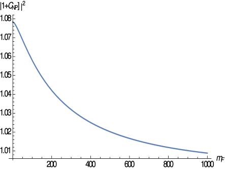
Figure 2: Plot of $|1+C_{NP}|^{2}$ vs $m_{F}$ for $m_{LQ}=900$ GeV and $m_{S}=150$ GeV.

The contribution from NP has reduced the deviation in $R(D^{*})$ from $3.4\sigma$ to $0.8\sigma$ and deviation in $R(D)$ from 2.3$\sigma$ to 0.6$\sigma$. In Figure 2 we plot $|1+C_{NP}|^{2}$ as a function of $m_{F}$ while fixing $m_{LQ}=900$ GeV and $m_{S}=150$ GeV. The NP contribution goes down as $m_{F}$ increases as shown in Figure 2 and falls to 1% of the SM value as $m_{F}\sim 1$ TeV.

The $(c,b)(\tau,\nu_{\tau})$ current can also contribute to $B_{c}\rightarrow\tau\nu_{\tau}$ with same $|1+C^{NP}|^{2}=1.04208$, however this is much smaller than the present allowed limit given as $|1+C^{NP}|_{allowed}^{2}=1.69$ RAlonso . Similarly NP contribution to $D_{s}\rightarrow\tau\nu_{\tau}$ is negligible compared to SM as well. Note that with the additional particle content of the model and their Yukawa interaction terms we also get NP contributions to hadronic decay of $\tau$. The decay $\tau\rightarrow(K\pi)\nu_{\tau}$ is proportional to the product of couplings $h_{s}^{\prime}h_{d}|h_{\tau}|^{2}$ and gives $C_{NP}^{\prime}=\mathcal{O}(10^{-6})$. Thus the NP contribution is quite small and negligible compared to SM contributions in this mode. Even though $h_{d}$ is complex, it still cannot contribute to the CP violation in $\tau\rightarrow(K\pi)\nu_{\tau}$ or $\tau\rightarrow\rho\pi\nu_{\tau}$ etc. This is because the NP contributions in this model to the vector and the axial-vector effective four current come with same magnitude and phase (see Ref. MyCP-paper ; MyCP-conf-paper and references there in for more details). NP contributions to $C_{9}$ in $B\rightarrow K^{(*)}\mu^{+}\mu^{-}$ via photon penguin is about $|C^{NP}_{9}|=3.428\times 10^{-3}$ which is again too small to have any effect on the reported anomaly in $C_{9}$ ACrivellin and NP contributions to $b\rightarrow s\gamma$ is $|C^{NP}_{7}+0.24C^{NP}_{8}|\approx 10^{-3}$ which is about two orders smaller than the 2$\sigma$ present experimental bound ACrivellin . In this model we can also get contributions to $B\rightarrow K^{(*)}\tau^{+}\tau^{-}$, $B_{s}\rightarrow\tau^{+}\tau^{-}$ and $D^{0}\rightarrow(\pi^{0})\nu_{\tau}\bar{\nu}_{\tau}$ which are not properly measured yet but NP contributions to these modes are less than a percent-level, at the order of $|1+C^{NP}_{2}|^{2}=1.0042$ or smaller and so negligible compared to the SM contribution. We also note that NP contribution to the anomalous magnetic moment of $\tau$ is $\Delta a^{NP}_{\tau}\approx-3.9\times 10^{-8}$ compared to the experimental bound $-0.052<\Delta a^{Exp.}_{\tau}<0.013$ PDG2016 which is again negligible.

III.2 Neutral meson oscillation.

Similar to the SM, the new particles in our model also contribute to neutral meson oscillations via the box loop. From the condition that we imposed in Eq.(5) our model gives no contribution to the $K^{0}-\bar{K}^{0}$ and $B^{0}-\bar{B}^{0}$. However for $B^{0}_{s}-\bar{B}^{0}_{s}$ oscillations we do have non vanishing contributions which can be put as

$$\mathcal{L}^{NP}_{eff}=2C_{B_{s}}^{NP}\bar{s_{\alpha}}\gamma^{\mu}P_{L}b_{\alpha}\bar{b_{\beta}}\gamma_{\mu}P_{L}s_{\beta}$$ (11)

where $C_{B_{s}}^{NP}=\frac{(h^{{}^{\prime}}_{s}h^{{}^{\prime}}_{b})^{2}}{128\pi^{2}m_{F}^{2}}S(x,x)$ where $S(x,x)$ are again the Inami-Lim functions with $x=\frac{m_{LQ}^{2}}{m_{F}^{2}}$ and the factor 2 to account for the contributions from the two diagrams in Figure 3.

Figure 3: Contributions to the $B^{0}_{s}-\bar{B}^{0}_{s}$ mixing from the new particles. The $F$ in the loop is the charged component of the vector-like lepton doublet.

Then introducing a factor of $\frac{1}{2!2!}$ to take into account the Wick contraction and color structure over counting, we have

$$\langle B^{0}_{s}|\bar{s_{\alpha}}\gamma^{\mu}P_{L}b_{\alpha}\bar{b_{\beta}}\gamma_{\mu}P_{L}s_{\beta}|\bar{B}^{0}_{s}\rangle=\frac{1}{4}\times\frac{1}{4}\times\frac{8}{3}M^{2}_{B^{0}_{s}}f^{2}_{B_{s}^{0}}B(\mu)\frac{1}{2M_{B^{0}_{s}}}$$ (12)

and so with $\Delta M_{B^{0}_{s}}^{NP}=2Re(\langle B^{0}_{s}|\mathcal{L}^{NP}_{eff}|\bar{B}^{0}_{s}\rangle$) we have

$$\Delta M_{B^{0}_{s}}^{NP}=\frac{1}{4\times 2}\times\frac{8}{3}M_{B^{0}_{s}}f^{2}_{B_{s}^{0}}B(\mu)\times C_{B_{s}}^{NP},$$ (13)

where $f_{B^{0}_{s}}$ is the $B^{0}_{s}$ decay form factor and $B(\mu)$ is a QCD scale correction factor, their values are taken from LDLuzio60 ; LDLuzio2018 .

Then with the values of the Yukawa couplings and masses given in the previous section we get $Re(\Delta M^{NP}_{B^{0}_{s}})=1.243$ ps^-1. This when compared to the error in experimental measurement of the same observable given as $\Delta M^{Exp}_{B^{0}_{s}}=(17.757\pm 0.021)$ ps^-1, the NP contribution is well above the error in the experimental measurement taken from PDG PDG2016 . But given that there are still large errors in the SM calculations with the latest estimate of SM calculation predicting a 1.8$\sigma$ deviation above the experimental average as $\Delta M^{SM}_{B^{0}_{s}}=(20.01\pm 1.25)$ ps^-1 LDLuzio2018 , the above NP contribution is well within the error in the latest SM calculation. We would like to point out that the previous SM calculations in Refs. LDLuzio60 ; LDLuzio61 agrees with the experimental value but their errors are larger than the latest SM prediction. Since NP contribution is allowed to be as large as the SM and experimental errors added in quadrature, if we take the previous SM predictions, NP contribution is allowed to be little larger than the above value. Note that in all the above calculations we have taken the hadronization parameters from Refs. LDLuzio60 ; LDLuzio2018 and the experimental values from PDG PDG2016 .

Due to $h_{d}$ being complex, we also have a non-zero imaginary component of $\Delta M^{NP}_{B^{0}_{s}}$ given as $Im(\Delta M^{NP}_{B^{0}_{s}})=-0.715\times\Gamma^{Exp}_{B^{0}_{s}}$. This can contribute to the CP violation in the $B^{0}_{s}-\bar{B}^{0}_{s}$ mixing which is parametrized in terms of $\frac{Re(\epsilon_{B^{0}_{s}})}{1+|\epsilon_{B^{0}_{s}}|^{2}}$, where $\epsilon_{B^{0}_{s}}=\frac{-\frac{1}{2}Im(\Delta M_{B^{0}_{s}})}{\frac{1}{2}\Delta\Gamma_{B^{0}_{s}}-i\Delta M_{B^{0}_{s}}}$. In our case with $\Delta\Gamma_{B^{0}_{s}}<<\Delta M_{B^{0}_{s}}$ the CP violating parameter due to NP can be approximately expressed as $\frac{Re(\epsilon^{NP}_{B_{s}^{0}})}{1+|\epsilon^{NP}_{B_{s}^{0}}|^{2}}\approx\frac{-Im(\Delta M^{NP}_{B_{s}^{0}})\times\Delta\Gamma^{Exp}_{B^{0}_{s}}}{4(\Delta M_{B^{0}_{s}}^{Exp})^{2}}\approx+1.050\times 10^{-5}$ compared to $\frac{Re(\epsilon^{Exp})}{1+|\epsilon^{Exp}|^{2}}\approx(-1.5\pm 7)\times 10^{-4}$ PDG2016 . Note that the NP contribution is an order of magnitude smaller than the present experimental limit. There is no contribution to the $\Delta\Gamma_{B^{0}_{s}}$ from NP since none of the intermediate particles in Figure 3 can go on shell. For the $D^{0}-\bar{D}^{0}$ oscillation with 2$\sigma$ bound from ACrivellin given as $|C^{Exp}_{D^{0}}|<2.7\times 10^{-7}$ $TeV^{-2}$ we compare $|C^{NP}_{D^{0}}|\approx 2.971\times 10^{-9}$ $TeV^{-2}$ and find the NP contribution to be around two orders of magnitude smaller than the present experimental bound at 2$\sigma$.

III.3 Z pole constrains.

For theoretical calculations of contribution from new fermions to the $Z$ decay into two fermions via higher order loops, we have used Chaing-Wei-Chang

$$Br(Z\rightarrow f_{i}f_{i})=\frac{G_{F}}{3\sqrt{2}\pi}\frac{m_{Z}^{3}}{(16\pi^{2})^{2}\Gamma^{tot.}_{Z}}(T^{i}_{3}-Q^{i}\sin^{2}(\theta_{W}))^{2}|h_{i}^{{}^{\prime}}|^{4}|[F_{2}(m_{F},m_{\phi})+F_{3}(m_{F},m_{\phi})]|^{2}$$ (14)

where

$$F_{2}(a,b)=\int^{1}_{0}dx(1-x)\ln{[(1-x)a^{2}+xb^{2}]}$$ (15)

and

$$F_{3}(a,b)= \int^{1}_{0}dx\int^{1-x}_{0}dy\frac{(xy-1)m_{Z}^{2}+(a^{2}-b^{2})(1-x-y)-\Delta\ln\Delta}{\Delta}$$ (16)

$$\Delta= -xym^{2}_{Z}+(x+y)(a^{2}-b^{2})+b^{2}$$ (17)

with $\Gamma^{tot}_{Z}=2.4952$.

Now with the numerical values of the Yukawa couplings given before and with $m_{F^{\pm}}=m_{F^{0}}=200$ GeV, $m_{\phi_{LQ}}=900$ GeV and $m_{S}=150$ GeV, we get $Br(Z\rightarrow\bar{d}d)_{NP}=0$ due to Eq. (5) while $Br(Z\rightarrow\bar{u}u)_{NP}$, $Br(Z\rightarrow\bar{s}s)_{NP}\,<<\,Br(Z\rightarrow\bar{c}c)_{NP}\approx\mathcal{O}(10^{-10})$ well within the experimental errors given by $Br(Z\rightarrow\bar{u}u)^{Exp}_{error}\approx 0.004$, $Br(Z\rightarrow\bar{s}s)^{Exp}_{error}\approx 0.004$ and $Br(Z\rightarrow\bar{c}c)^{Exp}_{error}\approx 0.0021$. Even for the decay mode where the large Yukawa choices can be significant we find $Br(Z\rightarrow\bar{b}b)_{NP}=4.737\times 10^{-5}$ as compared to $Br(Z\rightarrow\bar{b}b)^{Exp}_{error}\approx 5\times 10^{-4}$ putting the NP contribution an order of magnitude smaller than the experimental error. The contributions from NP to $Br(Z\rightarrow\bar{e}e)$ and $Br(Z\rightarrow\bar{\mu}\mu)$ are negligible compared to the experimental errors since we assume that $h_{e},\ h_{\mu}<<1$ (which is required to explain the $R(D^{(*)})$ anomalies). For the third generation lepton where we have $h_{\tau}$ large we get $Br(Z\rightarrow\bar{\tau}\tau)_{NP}\approx 7.62\times 10^{-9}$ and $Br(Z\rightarrow\bar{\nu}\nu(invisible))_{NP}\approx 2.47\times 10^{-8}$ compare to $Br(Z\rightarrow\bar{\tau}\tau)_{error}^{Exp}\approx 8\times 10^{-5}<Br(Z\rightarrow invisible)_{error}^{Exp}$. Here again the NP contributions are negligible. All the experimental values are taken from the latest PDG averages PDG2016 . Regarding the contributions of the new states Hong-Jian-He6 , to the Peskin-Tekeuchi S, T and U parameters, we find that with the above given masses of the new fermions we have $S\approx 0.0203$, $T\approx 0$ and $U\approx 0$ in our model, which are well within the present experimental bounds on these parameters Hong-Jian-He-2001 .

IV Conclusions.

In this work we have introduced a vector like fourth generation lepton doublet ($F^{0},\ F^{-}$) along with an $SU(3)_{c}$ triplet scalar leptoquark $\phi_{LQ}$ and a neutral scalar ($S$) both singlet under the $SU(2)_{L}$ gauge group. All the newly added particles are odd under a discrete symmetry $\mathcal{Z}_{2}$. With these new particles we have done a comprehensive analysis of the phenomenological consequences of the model taking all the very stringent constraints from $K^{0}-\bar{K^{0}}$ and $B^{0}_{i}-\bar{B^{0}_{i}}$ ($i=d,s$) oscillations as well as $Br(Z\rightarrow f\bar{f})$ and Peskin-Tekuchi parameters into account. We find that such a model can give a substantial contribution to $R(D^{(*)})$, and is able to reduce the tension between theoretical prediction and experimental measured value of $R(D^{*})$ from $3.4\sigma$ to $0.8\sigma$ and deviation in $R(D)$ from $2.3\sigma$ to $0.6\sigma$. Especially the NP contribution is able to reduce the discrepancy between experiment and theory in $R(D^{*})$ substantially. In addition the mass of the newly introduced states required to give a large contribution to the $R(D^{*})$ lie in a range which will be directly probed at the LHC with higher luminosity. Thus the model presents robust phenomenological consequences accessible at both the high energy collider experiment such as the LHC as well as leaving imprints in the flavor sector.

We find that while accommodating the large contributions to $R(D^{(*)})$ the model does not violate any other observations and is found to satisfy all other stringent constraints coming from neutral meson oscillations and precision Z-pole data.

References

• (1) C. W. Chang, H. Okada and E. Senaha, Phys. Rev. D 96, 015002 (2017).
• (2) C. Patrignani et al. (Particle Data Group), Chin. Phys. C, 40, 100001 (2016)
• (3) Lobsang Dhargyal, arXiv:1711.09772
• (4) Lobsang Dhargyal, Eur.Phys.J. C78 (2018) no.2, 150. arXiv:1709.04452
• (5) J. P Less et al. (BaBar Collaboration), Phys. Rev. D 88, 072012 (2013). arXiv:1303.0571
• (6) M. Huschle et al. (Belle Collaboration), Phys. Rev. D 92, 070214 (2015). arXiv:1507.03233
• (7) A. Abdesselam et al. (Belle Collaboration), arXiv:1603.06711
• (8) S. Hirose et al. (Belle Collaboration), arXiv:1612.00529
• (9) G. Wormser, $R(D^{*})$ status: overview and prospects; FPCP 2017 (talk)
• (10) R. Aaij et al. (LHCb Collaboration), Phys. Rev. Lett. 115, n. 11, 111803 (2015).
• (11) Y. Amhis et al., Eur. Phys. J. C77 (2017) 895; arXiv:1612.07233
• (12) H. Na et al., [HPQCD Collaboration], Phys. Rev. D 92, 054510 (2015)
• (13) J. F. Kamenik and F. Mescia, Phys. Rev. D 78, 014003 (2008)
• (14) D. Choudhury, A. Kundu, R. Mandal and R. Sinha, arXiv:1712.01593
• (15) T. Inami and C. S. Lim, Prog. Theor. Phys. 65 (1981) 297, [Erratum: Prog. Theor. Phys. 65.1772 (1981)]
• (16) P. Arnan, L. Hofer, F. Mescia and A. Crivellin, JHEP 1704 (2017) 043. arXiv:1608.07832
• (17) R. Alonso, B. Grinstein and J. M. Camalich, PRL 118, 081802 (2017), DOI:10.1103/PhysRevLett.118.081802
• (18) Lobsang Dhargyal, arXiv:1605.00629
• (19) Lobsang Dhargyal, arXiv:1610.06293
• (20) T. P. Cheng and L. F. Li, Gauge Theory of Elementary Particle Physics, Oxford University Press.
• (21) Elliot Leader and Enrico Predazzi, An introduction to gauge theories and modern particle physics. Volume 2. Cambridge University Press.
• (22) M. Artuso, G. Borissov and A. Lenz, Rev. Mod. Phys. 88 (4) (2016) 045002. arXiv:1511.09466
• (23) L. D. Luzio, M. Kirk and A. Lenz, arXiv:1712.06572
• (24) A. Lenz and U. Nierste, CKM 2010, Warwick, U.K, September 6-10, 2010.
• (25) M. E. Peskin and T. Takeuchi, Phys. Rev. Lett. 65, 964 (1990)
• (26) H. J. He, N. Polonsky and S. Su, Phys. Rev. D 64 (2001) 053004. arXiv:hep-ph/0102144v2