Two novel immunization strategies for epidemic control in directed scale-free networks with nonlinear infectivity

Abstract

In this paper, we propose two novel immunization strategies, i.e., combined immunization and duplex immunization, for SIS model in directed scale-free networks, and obtain the epidemic thresholds for them with linear and nonlinear infectivities. With the suggested two new strategies, the epidemic thresholds after immunization are greatly increased. For duplex immunization, we demonstrate that its performance is the best among all usual immunization schemes with respect to degree distribution. And for combined immunization scheme, we show that it is more effective than active immunization. Besides, we give a comprehensive theoretical analysis on applying targeted immunization to directed networks. For targeted immunization strategy, we prove that immunizing nodes with large out-degrees are more effective than immunizing nodes with large in-degrees, and nodes with both large out-degrees and large in-degrees are more worthy to be immunized than nodes with only large out-degrees or large in-degrees. Finally, some numerical analysis are performed to verify and complement our theoretical results. This work is the first to divide the whole population into different types and embed appropriate immunization scheme according to the characteristics of the population, and it will benefit the study of immunization and control of infectious diseases on complex networks.

Keywords: SIS model; Complex network; Combined immunization; Duplex immunization.

I Introduction

Devising effective immunization schemes is very important for the prevention and control of infectious diseases and computer viruses. For implement of an immunization scheme, when a portion of nodes (individuals) are immunized, those nodes can be thought as being removed from the network and cannot infect or be infected by others, then the tolerance of the network will be strengthened, so it is very important to choose key nodes to be immunized. In the previous works, studies are mainly focused on immunization schemes for susceptible-infected-susceptible (SIS) models BogunaM2011 ; Moreno2002 ; Pastor-Satorras2012 ; Fu2008 ; Pastor2001 ; Tanimoto2011 . The epidemic threshold characterizes the robustness of networks, and it signifies the critical value for a disease outbreak, when infection rate of an epidemic is beyond it, the epidemic will spread on the network, and an epidemic vanishes while the infection rate is below it. To increase the threshold, designing effective immunization strategies is very important Immunization2002 . Up to now, many effective immunization schemes have been proposed and studied, such as acquaintance immunization R2003 , random immunization Pastor-Satorras2012 , targeted immunization Pastor-Satorras2012 , active immunization Fu2008 , greedy immunization greedy2014 , dynamic immunization dynamic2015 , and so on.

Although many immunization strategies for epidemic models on complex networks have been studied extensively Pastor2001 ; Immunization2002 ; bai2007 ; R2003 ; R2004 ; M2004 , most of them are based on undirected networks Pastor-Satorras2012 ; Fu2008 . Real-world networks are closely related to directed networks, such as social networks, food webs, phone-call networks, the WWW www2003 , etc. The direction of nodes’ edges plays an important role in the study of epidemic spread on networks. Diseases, viruses or information spread out via their out-going edges and connect to others, while a susceptible node may be infected by its in-coming edges. Therefore, studying immunization strategies in directed networks is more practical and meaningful.

Many directed networks, such as the WWW www2003 and social networks, have power-law degree distributions of the form:

$P(k)=C_{1}k^{-2-\gamma}$ and $Q(l)=C_{2}l^{-2-\gamma^{{}^{\prime}}}$,

where $C_{1}$ and $C_{2}$ are normalization constants to guarantee $\sum_{k=m}^{M}P(k)=1$ and $\sum_{l=n}^{N}Q(l)=1$. Here we have $0<\gamma,\gamma^{{}^{\prime}}\leq 1$. Networks with power-law degree distributions are called scale-free. Here we suppose that $m$ is the minimal out-degree, $M$ the maximal out-degree, $n$ the minimal in-degree, and $N$ the maximal in-degree in the network.

In this paper, based on the heterogeneous mean-field theory Pastor2001 and degree distribution, we mainly study four immunization strategies for the SIS model on a directed network, including active immunization, targeted immunization, combined immunization and duplex immunization. We obtain the epidemic thresholds for these four immunization schemes, and compare effectiveness among them under the same immunization rate. Our results show that the proposed duplex immunization strategy is the most effective scheme among all usual immunization schemes, including proportional immunization, acquaintance immunization, targeted immunization, active immunization, and the proposed combined immunization. Besides, we divide the targeted immunization strategy into three cases in directed networks. We prove that nodes with large out-degrees are more important than nodes with large in-degrees when targeted immunization is implemented. On the other hand, we demonstrate that the nodes with both large in-degrees and large out-degrees are more worthy to be immunized than nodes with only large in-degrees or large out-degrees for targeted immunization scheme. To illustrate and test the performance of the proposed immunization schemes, we present numerical simulations in directed BA network in Figs 1-3, the numerical results are in accordance with our theoretical results.

The rest of the paper is organized as follows. In Section II, we establish an SIS model in a directed network and discuss epidemic thresholds with different infectivities. In Section III, we first study in detail the targeted immunization scheme in a directed network, then analyze the active immunization in a directed network. Besides, we propose two novel immunization strategies, and calculate the epidemic thresholds for them, and compare their effectiveness with targeted immunization and active immunization. In Section IV, we present numerical simulations. Finally, in Section V, we conclude the paper.

II The SIS Model in directed networks

In this section, we investigate the SIS model on a directed network. Nodes of the directed network are divided into two groups: Susceptible and Infected. Hereafter, we will denote a susceptible node by an S-node etc., for short. An S-node becomes infected at rate $\nu$ if it contacts with an infected individual, and an I-node may recover and become an S-node with probability $\delta$. Previous works have defined an effective spreading rate $\lambda=\frac{\nu}{\delta}$, where we take a unit recovery rate $\delta=1$. Let us denote the densities of S- and I-nodes with in-degrees $k$ and out-degrees $l$ at time $t$ by $s_{k,l}(t)$, $\rho_{k,l}(t)$, respectively, so we have

$s_{k,l}(t)+\rho_{k,l}(t)=1,$

where follows the joint probability distribution $p(k,l)$. Then, the respective marginal probability distribution of the out-degrees and in-degrees reads as

$P(k)=\underset{l}{\sum}p(k,l),~{}~{}Q(l)=\underset{k}{\sum}p(k,l),$

and their average degrees are

$\langle k\rangle=\underset{k,l}{\sum}kp(k,l)=\underset{k}{\sum}kP(k),~{}~{}\langle l\rangle=\underset{k,l}{\sum}lp(k,l)=\underset{l}{\sum}lQ(l).$

Then the SIS model can be written as the following ordinary differential equations:

$$\frac{d\rho_{k,l}}{dt}=\lambda k(1-\rho_{k,l}(t))\Theta(t)-\rho_{k,l}(t).$$ (1)

Here we suppose that the connectivity of nodes is uncorrelated, then the probability of a randomly selected outgoing link emanating form I-nodes at time $t$ is given by

$$\Theta(t)=\frac{\underset{k,l}{\sum}\varphi(k,l)p(k,l)\rho_{k,l}(t)}{\underset{k,l}{\sum}lp(k,l)}=\frac{\underset{k,l}{\sum}\varphi(k,l)p(k,l)\rho_{k,l}(t)}{{\langle l\rangle}},$$ (2)

where $\varphi(k,l)$ denotes the infectivity of a node with degrees $(k,l)$.

Now, we calculate the epidemic threshold for model (1). At the steady state, we have $\frac{d\rho_{k,l}}{dt}=0$ for all $k$ and $l$, from (1) we have

$$\rho_{k,l}=\frac{\lambda k\Theta}{1+\lambda k\Theta},$$

substituting the above equation into (2) we obtain a self-consistency equation for $\Theta$ as follows:

$$\Theta=\frac{1}{\langle l\rangle}\underset{k,l}{\sum}\frac{\lambda\varphi(k,l)p(k,l)k\Theta}{1+\lambda k\Theta}\equiv f_{1}(\Theta).$$

If this equation has a solution $\Theta>0$ other than $\Theta=0$, then it corresponds to an endemic state. Note that

$$f_{1}(1) = \frac{1}{\langle l\rangle}\underset{k,l}{\sum}\frac{\lambda\varphi(k,l)p(k,l)k}{1+\lambda k}<\frac{1}{\langle l\rangle}\underset{k,l}{\sum}lp(k,l)=1,$$

$$f^{\prime}_{1}(\Theta) = \frac{1}{\langle l\rangle}\underset{k,l}{\sum}\varphi(k,l)p(k,l)\frac{\lambda k}{(1+\lambda k\Theta)^{2}}>0,$$

$$f^{\prime\prime}_{1}(\Theta) = \frac{1}{\langle l\rangle}\underset{k,l}{\sum}\varphi(k,l)p(k,l)\frac{-2(\lambda k(1-\delta(k,l)))^{2}}{(1+\lambda k\Theta)^{3}}<0,$$

therefore, a nontrivial solution exists only if

$$\frac{df_{1}(\Theta)}{d\Theta}\bigg{|}_{\Theta=0}>1,$$ (3)

so we obtain the value of $\lambda$ yielding the inequality (3) which defines the critical epidemic threshold $\lambda_{c}$:

$$\lambda_{c}=\frac{\langle l\rangle}{\langle\varphi(k,l)k\rangle},$$ (4)

where the $\lambda_{c}$ is a critical value for the infection rate $\lambda$: If $\lambda>\lambda_{c}$, the disease will break out and persist on this network; Otherwise, when $\lambda<\lambda_{c}$, the disease will gradually peter out. Hence, it is very crucial to increase $\lambda_{c}$ on the network to prevent epidemic outbreak. We will give detailed analysis on this in Section III.

From the equality (4), we can see that the infectivity $\varphi(k,l)$ also affects the value of the threshold $\lambda_{c}$, so $\varphi(k,l)$ is also important for controlling the disease. For this reason, we give further study of the infectivity in the following subsection.

II.1 The epidemic threshold for the SIS model with nonlinear infectivity

For the SIS model on undirected scale-free networks Fu2008 , $\varphi(k)$ indicates the infectivity of a node with degree $k$. Previously, it was assumed that the larger the node degree, the larger the value of $\varphi(k)$, and in Pastor2001 ; Pastor2003 ; satorras2003 ; Pastor2002 , the $\varphi(k)$ is just equal to the node degree, that is, $\varphi(k)=k$, in this case, the epidemic threshold $\lambda_{c}=0$ when networks’ size is sufficiently large. However, in bai2007 ; yang2007 ; z2006 , the authors pointed out that large node with large $\varphi(k)$ is not always appropriate, so they assumed that $\varphi(k)=A$, where $A$ is a constant, and they obtained a different epidemic threshold $\lambda_{c}=\frac{1}{A}$, which is always positive. On the basis of this, in z2009 authors proposed a new nonlinear infectivity $\varphi(k)=\frac{ak^{\alpha}}{1+bk^{\alpha}}$, and analysis its threshold on finite and infinite networks.

Here in a directed scale-free network, we think both out-degrees and in-degrees play an important role in infectivity $\varphi(k,l)$. At the early stage of a disease transmission, a susceptible individual may get infected through out-going edges of infected individuals (in-coming edges of itself), then the disease spreads out of its out-going edges and connects to other susceptible nodes. When a susceptible individual has no in-coming edges, it cannot be infected by infected individuals; similarly, it will not infect other susceptible individuals without out-going edges even if it was infected.

Base on the analysis above, we give a nonlinear infectivity $\varphi(k,l)$ in a directed scale-free network as follows:

$$\varphi(k,l)=\frac{al^{\alpha}}{1+bl^{\alpha}}\cdot\frac{ck^{\beta}}{1+dk^{\beta}},$$ (5)

where $0\leq\alpha,\beta\leq 1,a>0$ and $b,c,d\geq 0$. In Eq. (5), when $k$ (or $l$) is very small, we can simply regard $\frac{ck^{\beta}}{1+dk^{\beta}}$ (or $\frac{al^{\alpha}}{1+bl^{\alpha}}$) as $0$, which means this node cannot infect others (or cannot be infected by others); and during the epidemic spreading process, the disease spreads out of infected individuals’ out-going edges, so the in-degrees of susceptible nodes is relatively more important than the out-degrees at the early stage, based on this, we choose $a>0$ rather than $a=0$; and here we divide the $\varphi(k,l)$ into four main cases:

(1)$\varphi(k,l)=\frac{ac}{(1+b)(1+d)}$ when $\alpha=0,\beta=0$, which means infectivity is a constant;

(2)$\varphi(k,l)=al$ when $\alpha=1,b,c=0$;

(3)$\varphi(k,l)=al^{\alpha}$ when $0<\alpha<1,b,c=0$;

(4)if $b,c\neq 0$, then $\varphi(k,l)=\frac{al^{\alpha}}{1+bl^{\alpha}}\cdot\frac{ck^{\beta}}{1+dk^{\beta}}$, and it becomes gradually saturated with the increasing of in-degree $k$ and out-degree $l$. Finally, it will converges to a constant $\varphi(k,l)=\frac{ac}{bd}$.

Substituting case (1) and case (2) into Eq. (4), we obtain two different epidemic thresholds as follows: $\lambda_{c}^{1}=\frac{ac\langle l\rangle}{(1+b)(1+c)\langle k\rangle}$ and $\lambda_{c}^{2}=\frac{1}{a\langle k\rangle}$, which were partially studied in w2012 ; and with sufficiently large $k$ and $l$, $\lambda_{c}^{1}=\frac{\langle ac\rangle}{\langle(1+b)(1+c)\rangle}$ and $\lambda_{c}^{2}=0$.

When $\varphi(k,l)=al^{\alpha}$ in case (3), we have $\langle\varphi(k,l)k\rangle=a\sum_{k}kP(k)\sum_{l}l^{\alpha}Q(l)$. By using a continuous approximation, we obtain

$$\langle k\varphi(k,l)\rangle=a\int_{m}^{\infty}\int_{m}^{\infty}k\cdot k^{-2-\gamma}\cdot l^{\alpha}\cdot l^{-2-\gamma^{\prime}}dkdl=a\int_{m}^{\infty}\frac{1}{k^{1+\gamma}}dk\cdot\int_{m}^{\infty}\frac{1}{l^{1+\gamma^{\prime}-\alpha}}dl.$$ (6)

From the above equation, we can conclude that the (6) is bounded when $\alpha<\gamma^{\prime}$. As a result, the epidemic threshold is

$$\lambda_{c}^{3}=\frac{m^{\gamma-\alpha}\gamma(1-\frac{\alpha}{\gamma^{\prime}})}{a},$$ (7)

which is always positive regardless of the size of out-degrees and in-degrees. We believe this is a interesting result, which is different from the result of a vanished threshold $\lambda_{c}=0$ given in Tanimoto2011 .

When $\varphi(k,l)=\frac{al^{\alpha}}{1+bl^{\alpha}}\cdot\frac{ck^{\beta}}{1+dk^{\beta}}$ , where we have $0<\alpha,\beta\leq 1$ and $b,d\neq 0$ in case(4), then

$$\langle k\varphi(k,l)\rangle=ac\sum_{k,l}p(k,l)k\frac{al^{\alpha}}{1+bl^{\alpha}}\cdot\frac{ck^{\beta}}{1+dk^{\beta}}=\int_{n}^{\infty}Q(l)\frac{al^{\alpha}}{1+bl^{\alpha}}\cdot\int_{m}^{\infty}P(k)\frac{ck^{\beta}}{1+dk^{\beta}},$$ (8)

similar to the above analysis in case (3), we can find that $\langle k\varphi(k,l)\rangle$ is always bounded, then we obtain that the threshold $\lambda_{c}^{4}$ is always a positive value.

Through analysis and calculation in this subsection, we obtain the different epidemic thresholds $\lambda_{c}^{i}~{}(i=1,2,3,4)$ for the four cases, and compare them with previous results. In Figs. 1-3, we present numerical analysis for different infectivities $\varphi(k,l)$, it clearly shows that the different infectivity $\varphi(k,l)$’s value result in different thresholds; and with nodes’ infectivity grows, $\lambda_{c}$ become smaller and smaller, so the network robustness against epidemics become weaker and weaker.

III The SIS model with immunization

From the analysis in Section II, we know that higher threshold $\lambda_{c}$ indicates better robustness against the outbreak of an epidemic on a network. Hence, designing an appropriate immunization strategy is important for effectively controlling the spread of the epidemic. And the SIS model is known as a more appropriate model than SIR model to study immunization schemes at the early time of epidemic transmission because the effects and recovery and death can be ignored, and this is the optimal time to apply immunization strategies in order to prevent and control epidemic outbreaks. In this section, we study the SIS model with various immunization strategies and compare their effectiveness among them for the same average immunization rate.

III.1 Targeted immunization in directed networks

The targeted immunization P2002 is known as the best strategy on heterogeneous networks, but we still lack a comprehensive understanding when applying it to directed networks. The traditional targeted immunization Pastor-Satorras2012 ; P2002 on undirected networks is to pick up the nodes with connectivity $k>\kappa$ to immunize, such as Eq.(14) in Fu2008 . In w2012 , Wang first studied the SIS model with targeted immunization in directed networks, but only immunize nodes with large out-degrees.

We realize that in the real-life systems with targeted immunization scheme, only select the large out-degree’s nodes to immunize w2012 may not always be appropriate. Beyond that, the in-degrees may also play a significant role in the epidemic immunization process; as we discussed in Section II, even the out-degrees of some nodes is very high, but those nodes may not always be infective with their in-degrees are too small. Otherwise, the nodes of high in-degrees with low out-degrees may not be infective as well.

So here we divide targeted immunization schemes into three cases to further compare their effectiveness: $(1)$ Immunize the nodes with $k>\pi_{1}$; $(2)$ Immunize the nodes with $l>\pi_{2}$; and $(3)$ Immunize the nodes with $k>\pi_{3}$ and $l>\pi_{4}$. Next in this subsection, we give a deep theoretical analysis on target immunization in directed networks under these three conditions, and to find an optimal one beyond them. Here we considere $\varphi(k,l)=A$ as a positive constant, we define the immunization rate $\delta_{k,l}^{i}(0<\delta_{k,l}^{i}\leq 1)$ by

$$\delta_{k,l}^{1}=\begin{cases}1,~{}k>\pi_{1}\\ a,~{}k=\pi_{1}~{},\\ 0,~{}k<\pi_{1}\end{cases}\delta_{k,l}^{2}=\begin{cases}1,~{}l>\pi_{2}\\ b,~{}l=\pi_{2}~{},\\ 0,~{}l<\pi_{2}\end{cases}\delta_{k,l}^{3}=\begin{cases}1,~{}k>\pi_{3}~{}~{}\mbox{and}~{}~{}l>\pi_{4}\\ c,~{}k=\pi_{3}~{}~{}\mbox{and}~{}~{}l=\pi_{4}~{},\\ 0,~{}\mbox{otherwise}\end{cases}$$ (9)

where $0<a,b,c\leq 1$, and $\underset{k,l}{\sum}\delta_{k,l}^{i}p(k,l)=\langle\delta_{k,l}^{i}\rangle$ $(i=1,2,3),$ and $\langle\delta_{k,l}^{i}\rangle$ are the average immunization rates. Then the epidemic dynamics model (1) becomes

$$\frac{d\rho_{k,l}}{dt}=\lambda k(1-\delta_{k,l})(1-\rho_{k,l}(t))\Theta(t)-\rho_{k,l}(t).$$ (10)

At the steady state, we have the condition $\frac{d\rho_{k,l}}{dt}=0$ for all $k$ and $l$. So we can get from (10) that

$$\rho_{k,l}=\frac{\lambda k(1-\delta_{k,l})\Theta}{1+\lambda k(1-\delta_{k,l})\Theta}.$$

Substituting these into Eq. 2, we obtain a self-consistency equation for $\Theta$ as follows:

$$\Theta=\frac{1}{\langle l\rangle}\underset{k,l}{\sum}\frac{\lambda\varphi(k,l)p(k,l)k(1-\delta_{k,l})\Theta}{1+\lambda k(1-\delta_{k,l})\Theta}\equiv f_{2}(\Theta),$$

therefore, we can obtain the threshold for model (10):

$$\hat{\lambda}_{c}=\frac{\langle l\rangle}{\langle\varphi(k,l)k\rangle-\langle\varphi(k,l)k\delta_{k,l}\rangle}.$$ (11)

Substituting (9) into (11) we obtain three epidemic thresholds with targeted immunization (1) (TGA), targeted immunization (2) (TGB) and targeted immunization (3) (TGC), respectively:

$$\hat{\lambda}_{c}^{1}=\frac{\langle l\rangle}{\langle\varphi(k,l)k\rangle-\langle\varphi(k,l)k\delta_{k,l}^{1}\rangle}=\frac{\langle l\rangle}{A(\langle k\rangle-\langle k\delta_{k,l}^{1}\rangle)},$$ (12)

$$\hat{\lambda}_{c}^{2}=\frac{\langle l\rangle}{\langle\varphi(k,l)k\rangle-\langle\varphi(k,l)k\delta_{k,l}^{2}\rangle}=\frac{\langle l\rangle}{A(\langle k\rangle-\langle k\delta_{k,l}^{2}\rangle)},$$ (13)

$$\hat{\lambda}_{c}^{3}=\frac{\langle l\rangle}{\langle\varphi(k,l)k\rangle-\langle\varphi(k,l)k\delta_{k,l}^{3}\rangle}=\frac{\langle l\rangle}{A(\langle k\rangle-\langle k\delta_{k,l}^{3}\rangle)}.$$ (14)

Higher epidemic thresholds indicates better performance of immunization schemes, through three epidemic thresholds (12)$-$(14), now we discuss the effectiveness of different targeted immunization schemes by comparing these three values: $\langle k\delta_{k,l}^{1}\rangle$, $\langle k\delta_{k,l}^{2}\rangle$ and $\langle k\delta_{k,l}^{3}\rangle$, the bigger one corresponds to better effectiveness.

Intuitively, we think the TGA is more effective than TGB, and the TGC is the optimal targeted immunization scheme in directed networks. During the immunization process, the in-coming links of the immunized S-nodes comes from the I-nodes and S-nodes itself, therefore, when we implement a target immunization on S-nodes, this in-coming links with $l>\pi_{2}$ comes from S-nodes itself which are harmless but are immunized at the same time, so the TGB may less effective than TGA.

In addition, as we explained in previous sections, the in-degrees also play a significant role in the immunization process, so it would be better to immunize the nodes with both large in-degrees and large out-degrees, which will be further discussed in this subsection.

Note that

$$\langle k\delta_{k,l}^{1}\rangle=\underset{k,l}{\sum}k\delta_{k,l}^{1}p(k,l)=\overset{M}{\underset{k=\pi_{1}}{\sum}}kP(k),~{}~{}~{}~{}~{}~{}~{}~{}~{}~{}$$

$$\langle k\delta_{k,l}^{2}\rangle=\underset{k,l}{\sum}k\delta_{k,l}^{2}p(k,l)=\overset{N}{\underset{l=\pi_{2}}{\sum}}Q(l)\overset{M}{\underset{k=m}{\sum}}kP(k),$$

$$\langle k\delta_{k,l}^{3}\rangle=\underset{k,l}{\sum}k\delta_{k,l}^{3}p(k,l)=\overset{N}{\underset{l=\pi_{4}}{\sum}}Q(l)\overset{M}{\underset{k=\pi_{3}}{\sum}}kP(k).$$

Under the same average immunization rate, which we take the average, then

$$\delta_{k,l}^{1}=\delta_{k,l}^{2}=\delta_{k,l}^{3} =\langle\delta_{k,l}^{1}\rangle=\langle\delta_{k,l}^{2}\rangle=\langle\delta_{k,l}^{3}\rangle$$ (15)

$$=\overset{M}{\underset{k=\pi_{1}}{\sum}}P(k)=\overset{N}{\underset{l=\pi_{2}}{\sum}}Q(l)=\overset{M}{\underset{k=\pi_{3}}{\sum}}\overset{N}{\underset{l=\pi_{4}}{\sum}}P(k)Q(l),$$

through the above equations, we have

$$\langle k\delta_{k,l}^{1}\rangle-\langle k\delta_{k,l}^{2}\rangle =\overset{M}{\underset{k=\pi_{1}}{\sum}}kP(k)-\overset{N}{\underset{l=\pi_{2}}{\sum}}Q(l)\overset{M}{\underset{k=m}{\sum}}kP(k)$$

$$=\overset{M}{\underset{k=\pi_{1}}{\sum}}kP(k)-\big{(}\overset{\pi_{1}-1}{\underset{k=m}{\sum}}kP(k)+\overset{M}{\underset{k=\pi_{1}}{\sum}}kP(k)\big{)}\overset{M}{\underset{k=\pi_{1}}{\sum}}P(k)$$

$$=\overset{M}{\underset{k=\pi_{1}}{\sum}}kP(k)\overset{\pi_{1}-1}{\underset{k=m}{\sum}}P(k)-\overset{\pi_{1}-1}{\underset{k=m}{\sum}}kP(k)\overset{M}{\underset{k=\pi_{1}}{\sum}}P(k)$$

$$=\overset{M}{\underset{\overline{k}=\pi_{1}}{\sum}}\overset{\pi_{1}-1}{\underset{k=m}{\sum}}\overline{k}P(\overline{k})P(k)-\overset{M}{\underset{\overline{k}=\pi_{1}}{\sum}}\overset{\pi_{1}-1}{\underset{k=m}{\sum}}kP(k)P(\overline{k})$$

$$=\overset{M}{\underset{\overline{k}=\pi_{1}}{\sum}}\overset{\pi_{1}-1}{\underset{k=m}{\sum}}P(\overline{k})P(k)\big{(}\overline{k}-k\big{)}$$

$$>0,$$

so it proves that the effectiveness of TGA is better than TGB.

Next, we discuss the effectiveness between TGC and TGA,TGB. Here, for better comparison, we set $\pi_{1}=\langle k\rangle$ , $\pi_{2}=\langle l\rangle$, and we find when $\pi_{3}>\langle k\rangle$ and $\pi_{4}>\xi$, where $\xi$ is a positive constant (can fetch its value as $\langle l\rangle$), the TGC is better than TGA and TGB.

Note that

$$\langle k\delta_{k,l}^{3}\rangle-\langle k\delta_{k,l}^{2}\rangle =\overset{N}{\underset{l=\pi_{4}}{\sum}}Q(l)\overset{M}{\underset{k=\pi_{3}}{\sum}}kP(k)-\overset{N}{\underset{l=\pi_{2}}{\sum}}Q(l)\overset{M}{\underset{k=m}{\sum}}kP(k)$$

$$=\overset{M}{\underset{k=\pi_{3}}{\sum}}\overset{N}{\underset{l=\pi_{4}}{\sum}}Q(l)kP(k)-\overset{M}{\underset{k=\pi_{3}}{\sum}}\overset{N}{\underset{l=\pi_{4}}{\sum}}Q(l)P(k)\overset{M}{\underset{k=m}{\sum}}kP(k)$$

$$=\overset{M}{\underset{k=\pi_{3}}{\sum}}\overset{N}{\underset{l=\pi_{4}}{\sum}}Q(l)P(k)\big{(}k-\overset{M}{\underset{k=m}{\sum}}kP(k)\big{)}$$

$$=\overset{M}{\underset{k=\pi_{3}>\langle k\rangle}{\sum}}\overset{N}{\underset{l=\pi_{4}}{\sum}}Q(l)P(k)\big{(}k-\langle k\rangle\big{)}$$

$$>0;$$

$$\langle k\delta_{k,l}^{3}\rangle-\langle k\delta_{k,l}^{1}\rangle =\overset{N}{\underset{l=\pi_{4}}{\sum}}Q(l)\overset{M}{\underset{k=\pi_{3}}{\sum}}kP(k)-\overset{M}{\underset{k=\pi_{1}}{\sum}}kP(k)~{}~{}~{}~{}~{}~{}~{}~{}~{}$$

$$=\overset{M}{\underset{k=\pi_{3}}{\sum}}kP(k)\frac{\overset{M}{\underset{k=\pi_{1}}{\sum}}P(k)}{\overset{M}{\underset{k=\pi_{3}}{\sum}}P(k)}-\overset{M}{\underset{k=\pi_{1}}{\sum}}kP(k)~{}~{}~{}~{}~{}~{}~{}~{}~{}$$

$$=\frac{\overset{M}{\underset{k=\pi_{3}}{\sum}}kP(k)\overset{M}{\underset{\widehat{k}=\pi_{1}}{\sum}}P(\widehat{k})-\overset{M}{\underset{k=\pi_{3}}{\sum}}P(k)\overset{M}{\underset{\widehat{k}=\pi_{1}}{\sum}}\widehat{k}P(\widehat{k})}{\overset{M}{\underset{k=\pi_{3}}{\sum}}P(k)}$$

$$=\frac{\overset{M}{\underset{k=\pi_{3}>\langle k\rangle}{\sum}}\overset{M}{\underset{\widehat{k}=\pi_{1}=\langle k\rangle}{\sum}}P(k)P(\widehat{k})\big{(}k-\widehat{k}\big{)}}{\overset{M}{\underset{k=\pi_{3}}{\sum}}P(k)}$$

$$>0,$$

therefore, the epidemic thresholds of TGC is greater than TGA’s and TGB’s, this means that the performance of TGC is better than TGA and TGB. Either the infectivity is linear or nonlinear, this conclusion is always valid. Figs. 2(c)-(d) and Figs. 3(c)-(d) below show this in details.

In this section, we divide the classic targeted immunization scheme into three cases in directed networks, the discussion and comparison of those three cases are carried out in depth. Now we have given the analytical comparison of the three different epidemic thresholds (see (12)$-$(14)). We prove that the nodes with both large in-degrees and large out-degrees are more worthy to be immunized during target immunization process in directed networks. Besides, immunizing nodes with large out-degrees are more efficient than immunizing nodes with large in-degrees for targeted immunization scheme.

III.2 Active immunization in directed networks

The classic active immunization Fu2008 is to immunize its neighbors with degrees $k\geq\kappa$ on undirected scale-free networks, here we will generalize it to directed networks and calculate its epidemic threshold. Then, the epidemic dynamics model becomes

$$\frac{d\rho_{k,l}}{dt}=\lambda k(1-\rho_{k,l}(t))\Theta(t)-(1+\overline{\delta}_{k,l})\rho_{k,l}(t),$$ (16)

where

$\overline{\delta}_{k,l}=\underset{k}{\sum}\frac{kP(k)}{\langle k\rangle}\delta_{k,l}^{1},$

and $\delta_{k,l}^{1}$ is defined in (9).

By adopting $\frac{d\rho_{k,l}}{dt}=0$ leads to

$$\Theta=\frac{\lambda\Theta}{\langle l\rangle}\sum_{k,l}\frac{k\varphi(k,l)p(k,l)}{\lambda k\Theta+1+\overline{\delta}_{k,l}}\equiv f_{3}(\Theta);$$

therefore, we obtain the epidemic threshold

$$\tilde{\lambda}_{c}=\frac{\langle l\rangle}{\sum_{k,l}(1+\overline{\delta}_{k,l})^{-1}k\varphi(k,l)p(k,l)}.$$

Note that

$$\overline{\delta}_{k,l}=\sum_{k}\frac{kP(k)}{\langle k\rangle}\delta_{k,l}^{1}=\frac{\langle k\delta_{k,l}^{1}\rangle}{\langle k\rangle},$$

we have

$$\tilde{\lambda}_{c}=\frac{\langle kl\rangle+\langle l\rangle\langle k\delta_{k,l}^{1}\rangle}{\langle k^{2}\varphi(k,l)\rangle}.$$ (17)

Compare (11) with (17), we have

$$\hat{\lambda}_{c}-\tilde{\lambda}_{c} =\frac{\langle l\rangle}{\langle\varphi(k,l)k\rangle-\langle\varphi(k,l)k\delta_{k,l}\rangle}-\frac{\langle kl\rangle+\langle l\rangle\langle k\delta_{k,l}^{1}\rangle}{\langle k^{2}\varphi(k,l)\rangle}$$

$$=\frac{\langle kl\rangle\langle\varphi(k,l)k\delta_{k,l}\rangle-\langle kl\varphi(k,l)\rangle\langle k\delta_{k,l}^{1}\rangle+\langle l\rangle\langle k\delta_{k,l}^{1}\rangle\langle\varphi(k,l)k\delta_{k,l}\rangle}{\big{(}\langle k^{3}\varphi^{2}(k,l)\rangle-\langle\varphi(k,l)k\delta_{k,l}\rangle\langle k^{2}\varphi(k,l)\rangle\big{)}}.$$ (18)

To better compare the target immunization and active immunization, we set the same average immunization rate

$$\overline{\delta}_{k,l}=\delta_{k,l},$$

therefore,

$$\frac{\langle k\delta_{k,l}^{1}\rangle}{\langle k\rangle}=\langle\delta_{k,l}\rangle.$$ (19)

From (18) and (19), we have

$$\hat{\lambda}_{c}-\tilde{\lambda}_{c}=\frac{\langle kl\rangle\langle\varphi(k,l)k\delta_{k,l}\rangle-\langle kl\varphi(k,l)\rangle\langle k\rangle\langle\delta_{k,l}\rangle+B}{A},$$ (20)

where $A=\langle k^{3}\varphi^{2}(k,l)\rangle-\langle\varphi(k,l)k\delta_{k,l}\rangle\langle k^{2}\varphi(k,l)\rangle$, and $B=\langle l\rangle\langle k\delta_{k,l}^{a}\rangle\langle\varphi(k,l)k\delta_{k,l}\rangle$.

Note that $\langle kl\varphi(k,l)\rangle\langle k\rangle\langle\delta_{k,l}\rangle=\langle kl\rangle\langle\varphi(k,l)k\delta_{k,l}\rangle+\sigma^{\prime}$. There may be appropriate small $\pi_{3}$, $\pi_{4}$, such that $\sigma^{\prime}$ is relatively smaller than $B$. So we can obtain that $\hat{\lambda}_{c}>\tilde{\lambda}_{c}$, which means that the target immunization scheme is more effective than active immunization under the same average immunization rate, Fig. 1(a) below illustrates this conclusion.

III.3 Combined immunization

In this section we propose a new immunization scheme, combined immunization: Choose a susceptible node and immunize its neighbors whose in-degrees $l>\kappa_{1}$, and choose an infected node to immunize its neighbors whose out-degrees $k>\kappa_{2}$ at the same time. Then the epidemic dynamics model becomes:

$$\frac{d\rho_{k,l}}{dt}=\lambda k(1-\rho_{k,l}(t))(1-\overline{\delta}_{l})\Theta(t)-(1+\overline{\delta}_{k})\rho_{k,l}(t),$$ (21)

where

$$\overline{\delta}_{l}=\underset{l}{\sum}\frac{lQ(l)}{\langle l\rangle}\delta_{l},\overline{\delta}_{k}=\underset{k}{\sum}\frac{kP(k)}{\langle k\rangle}\delta_{k},$$

$\delta_{l}=\begin{cases}1,~{}l>\kappa_{1}\\ d,~{}l=\kappa_{1}~{},\\ 0,~{}l<\kappa_{1}\end{cases}$ $\delta_{k}=\begin{cases}1,~{}k>\kappa_{2}\\ e,~{}k=\kappa_{2}~{},\\ 0,~{}k<\kappa_{2}\end{cases}$

and $0<d,e\leq 1$.

In the early stages of disease transmission, there may be quite a lot of susceptible individuals and infected individuals; therefore, to immunize them at the same time may be more appropriate. We show this rigorously below.

By letting $\frac{d\rho_{k,l}}{dt}=0$, than substitute it into (2), model (21) leads to

$$\Theta=\frac{\lambda\Theta}{\langle l\rangle}\underset{k,l}{\sum}\frac{k\varphi(k,l)p(k,l)(1-\overline{\delta}_{l})}{\lambda k(1-\overline{\delta}_{l})\Theta+1+\overline{\delta}_{k}}\equiv f_{4}(\Theta).$$

So the epidemic threshold for model (21) is

$$\bar{\lambda}_{c}=\frac{\langle l\rangle}{\underset{k,l}{\sum}(1+\overline{\delta}_{k})^{-1}k\varphi(k,l)p(k,l)(1-\overline{\delta}_{l})}.$$

Due to

$\overline{\delta}_{l}=\underset{l}{\sum}\frac{lQ(l)}{\langle l\rangle}\delta_{l}=\frac{\langle l\delta_{l}\rangle}{\langle l\rangle}$, $\overline{\delta}_{k}=\underset{k}{\sum}\frac{kP(k)}{\langle k\rangle}\delta_{k}=\frac{\langle k\delta_{k}\rangle}{\langle k\rangle}$.

We obtain that

$$\bar{\lambda}_{c}=\frac{\langle l^{2}\rangle(\langle k\rangle+\langle k\delta_{k}\rangle)}{\langle k^{2}\varphi(k,l)\rangle(\langle l\rangle-\langle l\delta_{l}\rangle)}.$$ (22)

Compare (22) with (4), we have

$$\bar{\lambda}_{c}=\lambda_{c}+\frac{\langle l^{2}\rangle\langle k\delta_{k}\rangle+\langle kl\rangle\langle l\delta_{l}\rangle}{\langle k^{2}\varphi(k,l)\rangle(\langle l\rangle-\langle l\delta_{l}\rangle)}>\lambda_{c}.$$ (23)

This means that the combined immunization scheme we propose here is indeed effective. Next we will compare the new immunization scheme with the active immunization scheme, through (22) and (17), we have

$$\bar{\lambda}_{c}-\tilde{\lambda}_{c} =\frac{\langle l^{2}\rangle(\langle k\rangle+\langle k\delta_{k}\rangle)}{\langle k^{2}\varphi(k,l)\rangle(\langle l\rangle-\langle l\delta_{l}\rangle)}-\frac{\langle kl\rangle+\langle l\rangle\langle k\delta_{k,l}^{1}\rangle}{\langle k^{2}\varphi(k,l)\rangle}$$

$$=\frac{\langle l^{2}\rangle\langle k\delta_{k}\rangle+\langle kl\rangle\langle l\delta_{l}\rangle+\langle l\rangle\langle l\delta_{l}\rangle\langle k\delta_{k,l}^{1}\rangle-\langle l^{2}\rangle\langle k\delta_{k,l}^{1}\rangle}{\langle k^{2}\varphi(k,l)\rangle(\langle l\rangle-\langle l\delta_{l}\rangle)}.$$ (24)

Setting the immunization rate as the same, so we have

$$\overline{\delta}_{l}+\overline{\delta}_{k}=\overline{\delta}_{k,l},$$

where $\overline{\delta}_{k,l}$ is defined in Section III.2 and $\overline{\delta}_{l},\overline{\delta}_{k}$ are defined in Section III.3. Therefore,

$$\frac{\langle l\delta_{l}\rangle}{\langle l\rangle}+\frac{\langle k\delta_{k}\rangle}{\langle k\rangle}=\frac{\langle k\delta_{k,l}^{1}\rangle}{\langle k\rangle}.$$ (25)

From (24) and (25) we obtain that

$$\bar{\lambda}_{c}-\tilde{\lambda}_{c} =\frac{\langle l\delta_{l}\rangle\big{(}\langle l\rangle\langle k\delta_{k}\rangle+\langle k\rangle\langle l\delta_{l}\rangle\big{)}}{\langle k^{2}\varphi(k,l)\rangle(\langle l\rangle-\langle l\delta_{l}\rangle)}$$

$$>0,$$ (26)

as it is obvious that $\langle l\rangle>\langle l\delta_{l}\rangle$.

That is to say, under the same average immunization rate, the combined immunization is more effective than the active immunization discussed in Section III.2. Fig. 1(b) below illustrates this conclusion.

Considering (23) and (14), under the same average immunization $\frac{\langle l\delta_{l}\rangle}{\langle l\rangle}+\frac{\langle k\delta_{k}\rangle}{\langle k\rangle}=\langle\delta_{k,l}^{3}\rangle$, we have

$$\bar{\lambda}_{c}=\frac{\langle l^{2}\rangle(\langle k\rangle+\langle k\delta_{k}\rangle)(\langle\varphi(k,l)k\rangle-\langle\varphi(k,l)k\delta_{k,l}^{3}\rangle)}{\langle k^{2}l\varphi(k,l)\rangle(\langle l\rangle-\langle l\delta_{l}\rangle)}\hat{\lambda}_{c}^{3}.$$

Note that

$$\langle l^{2}\rangle(\langle k\rangle+\langle k\delta_{k}\rangle)(\langle\varphi(k,l)k\rangle-\langle\varphi(k,l)k\delta_{k,l}^{3}\rangle)>0,$$

$$\langle k^{2}l\varphi(k,l)\rangle(\langle l\rangle-\langle l\delta_{l}\rangle)>0.$$

So $\bar{\lambda}_{c}=\Lambda\hat{\lambda}_{c}^{3}$, where $\Lambda$ is a positive constant, which means that the combined immunization scheme is comparable in effectiveness to the targeted immunization scheme discussed in Section III.1.

III.4 Duplex immunization

Infected individuals play a vital part in the early stages of disease transmission, diseases spread through out-going links of infected individuals to the in-coming links of susceptible individuals. Therefore the out-degree $l$ is a key character during the early stage of a disease transmission. And all immunization strategies Pastor2001 ; Pastor2003 ; satorras2003 ; Pastor2002 ; bai2007 consider the all nodes as a whole to implement the immunization strategies, so in this section we proposed an immunization strategy based on a partition of the out-degrees $l$; we divide the population of all nodes with out-degrees $l$ and in-degrees $k$ into two parts: Nodes with out-degrees exceeding a positive constant number $L$ is considered as the first part $T=\{(k,l)|l>L$}; and $\overline{T}$, the complement of $T$, as the second part. In $\overline{T}$, we use the targeted immunization in Section III.1, and in $\overline{T}$, we use the combined immunization proposed in Section III.2. It turns out that the effectiveness of these two immunization strategies’ combination is more effective than both of them.

We introduce a constant $\alpha\in[0,1]$, which indicates the proportion of set $\overline{T}$, so we have

$s_{k,l}(t)+\rho_{k,l}(t)=\begin{cases}\alpha,&\mbox{if}~{}~{}(k,l)\in\overline{T},\\ 1-\alpha,&\mbox{if}~{}~{}(k,l)\in T.\end{cases}$

The condition $\alpha=1$ implies the classic targeted immunization (1) in Section III.1 , while $\alpha=0$ means the combined immunization proposed in Section III.3, implementing two kinds of immunization strategies together, the model (1) becomes

$$\frac{d\rho_{k,l}}{dt}=\begin{cases}\lambda k(1-\widehat{\delta}_{k})(\alpha-\rho_{k,l}(t))\theta(t)-\rho_{k,l}(t),&\mbox{if}~{}~{}(k,l)\in\overline{T},\\ \lambda k(1-\alpha-\rho_{k,l}(t))(1-\overline{\delta}_{l^{\prime}})\theta(t)-(1+\overline{\delta}_{k^{\prime}})\rho_{k,l}(t),&\mbox{if}~{}~{}(k,l)\in T.\end{cases}$$ (27)

where

$$\overline{\delta}_{l^{\prime}}=\underset{l}{\sum}\frac{lQ(l)}{\langle l\rangle}\delta_{l^{\prime}},~{}\overline{\delta}_{k^{\prime}}=\underset{k}{\sum}\frac{kP(k)}{\langle k\rangle}\delta_{k^{\prime}},$$

and

$\widehat{\delta}_{k}=\begin{cases}1,~{}k>\eta_{1}\\ a^{\prime},~{}k=\eta_{1}~{},\\ 0,~{}k<\eta_{1}\end{cases}$ $\delta_{l^{\prime}}=\begin{cases}1,~{}l>\eta_{2}\\ b^{\prime},~{}l=\eta_{2}~{},\\ 0,~{}l<\eta_{2}\end{cases}$ $\delta_{k^{\prime}}=\begin{cases}1,~{}k>\eta_{3}\\ c^{\prime},~{}k=\eta_{3}~{},\\ 0,~{}k<\eta_{3}\end{cases}$

where $0<a^{\prime},b^{\prime},c^{\prime}\leq 1$, and $\eta_{2}\geq L$.

By letting $\frac{d\rho_{k,l}}{dt}=0$, than substitute it into (2), model (27) leads to a self-consistency equation:

$$\Theta=\frac{\lambda\Theta}{\langle l\rangle}\left\{\underset{k,l}{\sum}\frac{\alpha\lambda\varphi(k,l)p(k,l)k(1-\widehat{\delta}_{k})}{1+\lambda k(1-\widehat{\delta_{k}})\Theta}+\underset{k,l}{\sum}\frac{(1-\alpha)k\varphi(k,l)p(k,l)(1-\overline{\delta}_{l^{\prime}})}{\lambda k(1-\overline{\delta}_{l^{\prime}})\Theta+1+\overline{\delta}_{k^{\prime}}}\right\}\equiv f_{5}(\Theta),$$

therefore, we can obtain the epidemic threshold for model (27):

$$\check{\lambda}_{c}=\frac{\langle l\rangle}{\alpha\big{(}\langle\varphi(k,l)k\rangle-\langle\varphi(k,l)k\widehat{\delta}_{k}\rangle\big{)}}+\frac{\langle l^{2}\rangle(\langle k\rangle+\langle k\delta_{k^{\prime}}\rangle)}{(1-\alpha)\langle k^{2}\varphi(k,l)\rangle(\langle l\rangle-\langle l\delta_{l^{\prime}}\rangle)},$$ (28)

which is clearly greater than the epidemic threshold $\lambda_{c}$ obtained in (4), that means the immunization scheme we proposed is indeed effective.

In Section III.1, we know that the TGC is more effective than TGA and TGB, and through Section III.2, we find the combined immunization is more effective than the active immunization.

We now compare the new immunization scheme, the duplex immunization, with the TGC and the combined immunization to find the optimal one.

Through (28) and (14), we have

$$\check{\lambda}_{c}-\hat{\lambda}_{c}^{3} =\frac{\langle l\rangle}{\alpha\big{(}\langle\varphi(k,l)k\rangle-\langle\varphi(k,l)k\widehat{\delta}_{k}\rangle\big{)}}+\frac{\langle l^{2}\rangle(\langle k\rangle+\langle k\delta_{k^{\prime}}\rangle)}{(1-\alpha)\langle k^{2}\varphi(k,l)\rangle(\langle l\rangle-\langle l\delta_{l^{\prime}}\rangle)}-\frac{\langle l\rangle}{\langle\varphi(k,l)k\rangle-\langle\varphi(k,l)k\delta_{k,l}^{3}\rangle}$$

$$=\frac{1}{A^{*}}\big{(}B^{*}+C^{*}-D^{*}\big{)},$$

where

$$A^{*} = \alpha(1-\alpha)\langle k^{2}\varphi(k,l)\rangle(\langle l\rangle-\langle l\delta_{l^{\prime}}\rangle)(\langle\varphi(k,l)k\rangle-\langle\varphi(k,l)k\widehat{\delta}_{k}\rangle)(\langle\varphi(k,l)k\rangle-\langle\varphi(k,l)k\delta_{k,l}^{3}\rangle),$$

$$B^{*} = =\langle l\rangle(1-\alpha)\langle k^{2}\varphi(k,l)\rangle(\langle l\rangle-\langle l\delta_{l^{\prime}}\rangle)(\langle\varphi(k,l)k\rangle-\langle\varphi(k,l)k\delta_{k,l}^{3}\rangle),$$

$$C^{*} = \alpha(\langle\varphi(k,l)k\rangle-\langle\varphi(k,l)k\widehat{\delta}_{k}\rangle)\langle l^{2}\rangle(\langle k\rangle+\langle k\delta_{k^{\prime}}\rangle)(\langle\varphi(k,l)k\rangle-\langle\varphi(k,l)k\delta_{k,l}^{3}\rangle),$$

$$D^{*} = \langle l\rangle(1-\alpha)\alpha\langle k^{2}\varphi(k,l)\rangle(\langle l\rangle-\langle l\delta_{l^{\prime}}\rangle)(\langle\varphi(k,l)k\rangle-\langle\varphi(k,l)k\widehat{\delta}_{k}\rangle).$$

It is obvious that these four polynomials: $A^{*}$, $B^{*}$, $C^{*}$ and $D^{*}$ are greater than zero. For $\overline{T}$, the average immunization rate is $\alpha\langle\widehat{\delta}_{k}\rangle$; For $T$, the average immunization rate is $(1-\alpha)(\frac{\langle l\delta_{l^{\prime}}\rangle}{\langle l\rangle}+\frac{\langle k\delta_{k^{\prime}}\rangle}{\langle k\rangle})$; hence, under the same average immunization rate for duplex immunization and TGC, we have

$$(1-\alpha)(\frac{\langle l\delta_{l^{\prime}}\rangle}{\langle l\rangle}+\frac{\langle k\delta_{k^{\prime}}\rangle}{\langle k\rangle})+\alpha\langle\widehat{\delta}_{k}\rangle=\langle\delta_{k,l}^{3}\rangle.$$ (29)

Note that

$$B^{*}-D^{*}=\langle l\rangle(1-\alpha)\langle k^{2}\varphi(k,l)\rangle(\langle l\rangle-\langle l\delta_{l^{\prime}}\rangle)\big{(}\langle\varphi(k,l)k\rangle-\langle\varphi(k,l)k\delta_{k,l}^{3}\rangle-\alpha(\langle\varphi(k,l)k\rangle-\langle\varphi(k,l)k\widehat{\delta}_{k}\rangle)\big{)}.$$ (30)

Combining (29) and (30), we obtain that when $\alpha$ satisfies the condition: $\alpha<E^{*}<1$, then

$$\check{\lambda}_{c}>\hat{\lambda}_{c}^{3},$$ (31)

where $E^{*}=(\langle\varphi(k,l)k\rangle-\langle\varphi(k,l)k\delta_{k,l}^{3}\rangle)/(\langle\varphi(k,l)k\rangle-\langle\varphi(k,l)k\widehat{\delta}_{k}\rangle)$, which means that the duplex immunization scheme is more effective than the target immunization scheme discussed in Section III.1.

With the similar analysis method above, we can verify that the duplex immunization scheme is more effective than the combined immunization scheme discussed in Section III.3. Fig. 1(a) below shows $\check{\lambda}_{c}>\bar{\lambda}_{c}$ very clearly with the same average immunization rate $\delta=0.12$, and this result applies to all same $\delta$.

Besides, through Fu2008 ; w2012 , we know the targeted immunization scheme is more effective than proportional immunization scheme and acquaintance immunization scheme for the same average immunization rate in directed networks. Hence, we reach the following conclusion: The duplex immunization we proposed has the best effectiveness comparing to all other usual immunization schemes with respect to degree distribution in directed scale-free networks.

III.5 A brief summary

In the previous section, we have discussed targeted, active, combined and duplex immunization schemes, and calculated the thresholds for these strategies. By comparing the thresholds for different immunization strategies, we have conclude that the epidemic threshold of TGB (see Eq. (13)) is greater than that of TGA (see Eq. (12)); Then we proved that the targeted nodes with both large in-degrees and large out-degrees (see Eq. (14)) are more worthy to be immunized in directed networks; We extended the traditional active immunization Fu2008 into directed networks, analyzed its epidemic threshold and compared its effectiveness with targeted immunization scheme and combined immunization scheme under the same average immunization rate; The proposed combined immunization scheme is more effective than active immunization scheme, and it is comparable to the targeted immunization scheme; And the performance of the duplex immunization scheme is the best among all usual immunization schemes discussed in this section.

IV Numerical analysis

In this section, we present the results of numerical simulations to further illustrate the above theoretical analysis and show the effectiveness of different immunization schemes. We use the algorithm of Barabási and Albert R2002 to generate a directed scale-free network with $\gamma=1$ and $\gamma^{{}^{\prime}}=1$. Here the joint degree distribution is independent, we consider a population of 1000 individuals and take a unit recovery rate.

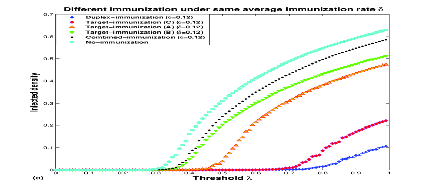
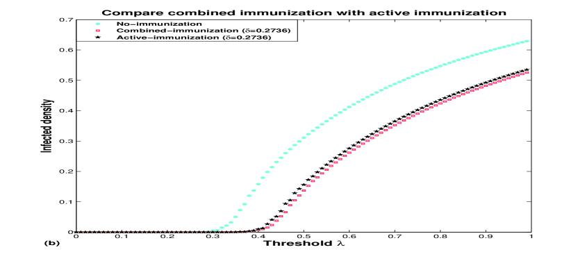
Figure 1: (Color online) Comparison of the effectiveness of different immunization schemes under the same average immunization rate $\delta$. (a) shows the thresholds among those five immunization schemes under the average immunization rate $\delta=0.12$, the threshold $\lambda_{c}=0.25$ for no immunization, the threshold $\bar{\lambda}_{c}=0.27$ for combined immunization, the threshold $\hat{\lambda}_{c}^{2}=0.29$ for TGB, the threshold $\hat{\lambda}_{c}^{1}=0.4$ for TGA, the threshold $\hat{\lambda}_{c}^{3}=0.6$ for TGC, the threshold $\check{\lambda}_{c}=0.7$ for duplex immunization. (b) shows that the combined immunization scheme is more effective than the active scheme for the same average immunization rate $\delta=0.2736$, the threshold $\tilde{\lambda}_{c}=0.32$ for active immunization and $\bar{\lambda}_{c}=0.35$ for combined immunization.

In Fig. 1(a), we repeated the simulation above when the immunization schemes-targeted (1, 2, 3), combined and duplex-are implemented. We set the same average immunization rate for these five immunization schemes to better compare their effectiveness with each other, and we implement a no-immunization curve for all immunization schemes to illustrate that all immunization schemes are effective comparing to the case without any immunization. The average out-degree ($\langle k\rangle$) and average in-degree ($\langle l\rangle$) for the generated network is 3 and 5, respectively, and $k_{max}=82,l_{max}=100$. Here we set the infectivity as a constant $\varphi(k,l)=2$. For TGA we choose $\pi_{1}=7$ and $a=1$, for TGB we choose $\pi_{2}=4$ and $b=1$, and for TGC we choose $\pi_{3}=4$, $\pi_{4}=2$ and $c=1$. We can see in Fig. 1(a), under the same average immunization rate $\delta=0.12$, $\hat{\lambda}_{c}^{3}>\hat{\lambda}_{c}^{1}>\hat{\lambda}_{c}^{2}$, which means the performance of TGC is better than TGA and TGB. And for the targeted immunizations on a directed scale-free network, to immunize nodes with large out-degrees is more efficient than to immunize nodes with large in-degrees.

Besides, we can obtain the epidemic threshold for duplex immunization $\check{\lambda}_{c}=0.7$ and $\hat{\lambda}_{c}^{3}=0.6$ of TGC, which verifies the conclusion in Section III.4, and means that the duplex immunization we proposed is more effective than the targeted immunization discussed in III.1 for the same average immunization rate. Here we take $T=\{(k,l)|l>2$}, $\eta_{1}=17$, $a^{\prime}=1$, $\eta_{2}=18$, $b^{\prime}=1$, $\eta_{3}=10$, $c^{\prime}=1$, and $\alpha$ can be calculated as $0.6188$. When infectivity takes linear or nonlinear function, in Figs. 2(c-d) and Figs. 3(c-d), those conclusions are still valid.

In Fig. 1(b), we compare the thresholds among no immunization, active and combined immunization schemes; we set the same average immunization rate $\delta=0.2736$ for those two immunization schemes. Here $\pi_{1}=9$ for active immunization scheme, and $\kappa_{1}=15,\kappa_{2}=13$ for combined immunization scheme. So we can illustrate the conclusion in Section III.3 (see Eq. 26), which means that the combined immunization scheme proposed in Section III.3 is more effective than the active immunization scheme discussed in Section III.2 for the same average immunization rate.

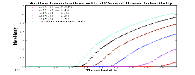
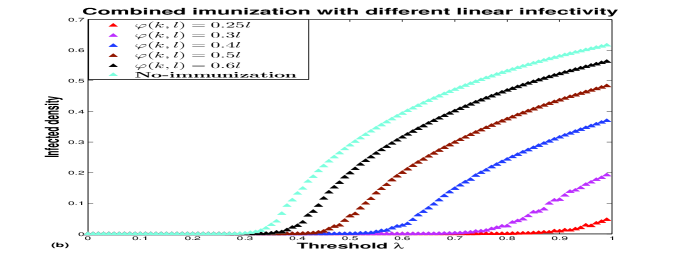
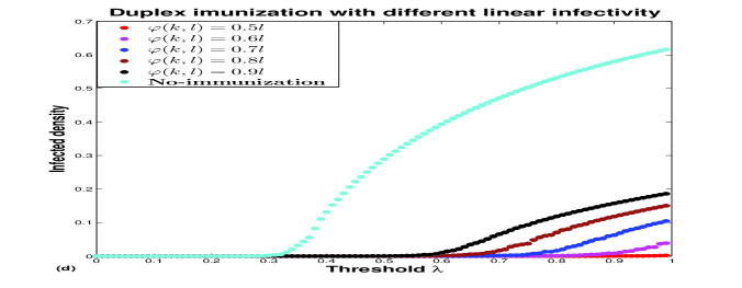
Figure 2: (Color online) Different linear infectivity $\varphi(k,l)$’s effects on four immunization schemes. We take linear infectivity $\varphi(k,l)=al$, in (a) and (b), $a=0.25,0.3,0.4,0.5,0.6$; in (c) and (d), $a=0.5,0.6,0.7,0.8,0.9$.

In Fig. 2, we choose a linear infectivity $\varphi(k,l)=al$ and set the same $\delta=0.12$. For active and combined immunization schemes, we set $a=0.25,0.3,0.4,0.5,0.6$, and for targeted immunization(c) and duplex immunization, we set $a=0.5,0.6,0.7,0.8,0.9$. Still, in Figs. 2(a)-(d), we take the same average immunization rate $\delta=0.12$. The Figs. 2(a)-(d) clearly show that with an increasing $a$, the thresholds of those four immunization schemes are increasing at the same time; on the other hand, with different linear infectivity, the duplex immunization is still more effective than targeted immunization, and the combined immunization is still more effective than active immunization.

In Fig. 3, we choose a nonlinear infectivity $\varphi(k,l)=al^{\alpha}$. For active and combined immunization, we set $a=0.6$, $\alpha=0.5,0.6,0.7,0.8,09$ and for targeted immunization(c) and duplex immunization, we set $a=0.85$, $\alpha=0.5,0.6,0.7,0.8,09$ . We choose $\delta=0.12$ in Figs. 3(a)-(d), which shows the similar property when infectivity is linear: when $\alpha$ increases, threshold increases. And by different nonlinear infectivity, the thresholds changes faster than linear infectivity. Besides, with different nonlinear infectivity for same immunization rate, the duplex immunization is more effective than targeted immunization and the combined immunization is more effective than active immunization.

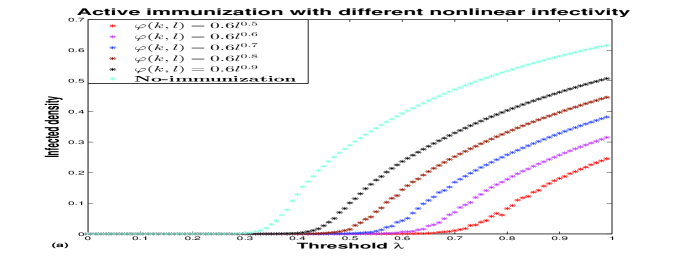
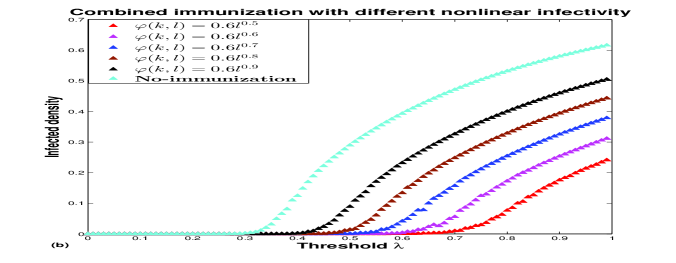
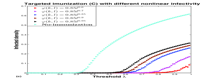
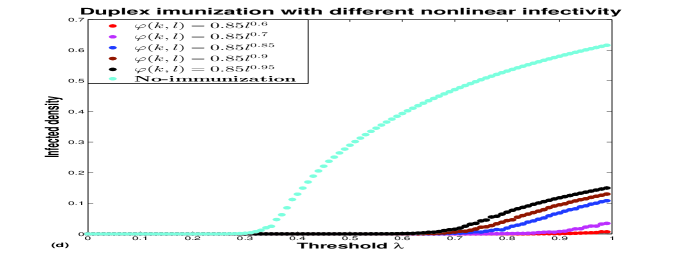
Figure 3: (Color online) Different nonlinear infectivity $\varphi(k,l)$’s effects on four immunization schemes. We take nonlinear infectivity $\varphi(k,l)=al^{\alpha}$, in (a) and (b), $a=0.6$, $\alpha=0.5,0.6,0.7,0.8,0.9$; in (c) and (d), $a=0.85$, $\alpha=0.6,0.7,0.85,0.9,0.95$.

In addition, in Fig. 1, we present the contrast among different immunization strategies for the same immunization rate and validate that the duplex immunization is more effective than targeted immunization; the performance of combined immunization is better than active immunization. In Figs. 2-3, we use different linear and nonlinear infectivities $\varphi(k,l)$ on active, combined, targeted and duplex immunization schemes, it is shown that with higher infectivity, the epidemic threshold is dramatically reduced; besides, the results of comparison between those immunization schemes are still valid with different linear and nonlinear infectivities.

V Conclusions and discussions

In this paper, different immunization strategies for SIS models in directed scale-free networks with different infectivities are studied, and we calculate the epidemic thresholds for different immunization schemes, and obtained the following results:

Firstly, the epidemic threshold $\lambda_{c}$ takes a positive value if $\varphi(k,l)=al^{\alpha}$ and $\alpha<\gamma^{\prime}$ in a finite network with sufficiently large size; besides, when $\varphi(k,l)=\frac{al^{\alpha}}{1+bl^{\alpha}}\cdot\frac{ck^{\beta}}{1+dk^{\beta}}$, $\lambda_{c}$ is always positive.

Secondly, for the targeted immunization in directed networks, we prove that immunizing nodes with large out-degrees are more effective than immunizing nodes with large in-degrees when targeted immunization is implemented; on the other hand, we demonstrate that the nodes with both large in-degrees and large out-degrees are more worthy to be immunized during target immunization process than nodes with only large in-degrees or large out-degrees.

Thirdly, the duplex immunization we proposed has the best effectiveness comparing to all other usual immunization schemes (e.g., proportional immunization, acquaintance immunization, targeted immunization, active immunization, and combined immunization) for the same average immunization rate. Besides, the performance of the combined immunization we proposed on disease control is better than active immunization.

Finally, from realistic viewpoints, weighted networks and degree-correlated networks are more reasonable for epidemic immunization, and we expect that our work may be extended into these and even multiplex and interconnected networks in our future research.

Acknowledgements

This work was jointly supported by the NSFC under grants 11572181 and 11331009.

References

• (1) Bogun$\acute{a}$ M, Pastor-Satorras R, Vespignani A. Epidemic spreading in complex networks with degree correlations[M]. in Statistical Mechanics of Complex Networks, Springer, Berlin, Heidelberg, 2003: 127-147.
• (2) Moreno Y, Pastor-Satorras R, Vespignani A. Epidemic outbreaks in complex heterogeneous networks[J]. European Physical Journal B, 2002, 26(4): 521-529.
• (3) Pastor-Satorras R, Vespignani A. Epidemics and immunization in scale-free networks[J]. arXiv preprint cond-mat/0205260, 2002.
• (4) Fu X C, Small M, Walker D M, et al. Epidemic dynamics on scale-free networks with piecewise linear infectivity and immunization[J]. Physical Review E, 2008, 77(3): 036113.
• (5) Wang Q, Zhu G H, Fu X C. Comparison of epidemic thresholds on directed networks and immunization analysis[J]. Complex Systems & Complexity Science, 2012, 9(4):26-33. (In Chinese)
• (6) Pastor-Satorras R, Vespignani A. Immunization of complex networks[J]. Physical Review E, 2002, 65(3 Pt 2A):036104.
• (7) Tanimoto S. Epidemic thresholds in directed complex networks[J]. arXiv preprint arXiv:1103.1680, 2011.
• (8) Albert R, Barab$\acute{a}$si A L. Statistical mechanics of complex networks[J]. Reviews of Modern Physics, 2002, 74(1): 47.
• (9) Pastor-Satorras R, Vespignani A. Epidemic spread in scale-free networks[J]. Physical Review Letters, 2001, 86(14): 3200.
• (10) Bogun$\acute{a}$ M, Pastor-Satorras R, Vespignani A. Absence of epidemic threshold in scale-free networks with degree correlations[J]. Physical Review Letters, 2003, 90(2): 028701.
• (11) Pastor-Satorras R, Vespignani A. Epidemic dynamics and endemic states in complex networks[J]. Physical Review E, 2001, 63(6): 066117.
• (12) Pastor-Satorras R, Vespignani A. Epidemic dynamics in finite size scale-free networks[J]. Physical Review E, 2002, 65(3): 035108.
• (13) Bai W J, Zhou T, Wang B H. Immunization of susceptible-infected model on scale-free networks[J]. Physica A, 2007, 384(2): 656-662.
• (14) Yang R, Wang B H, Ren J, et al. Epidemic spreading on heterogeneous networks with identical infectivity[J]. Physics Letters A, 2007, 364(3-4): 189-193.
• (15) Zhou T, Liu J G, Bai W J, et al. Behaviors of susceptible-infected epidemics on scale-free networks with identical infectivity[J]. Physical Review E, 2006, 74(5): 056109.
• (16) Zhang H F, Fu X C. Spreading of epidemics on scale-free networks with nonlinear infectivity[J]. Nonlinear Analysis TMA, 2009, 70(9): 3273-3278.
• (17) Cohen R, Havlin S, Ben-Avraham D. Efficient immunization strategies for computer networks and populations[J]. Physical Review Letters, 91(2003) 247901
• (18) Liu Z H, Chen G L, Wang N N, et al. Greedy immunization strategy in weighted scale-free networks[J]. Engineering Computations, 2014, 31(8): 1627-1634.
• (19) Wu Q C, Fu X C, Jin Z, et al. Influence of dynamic immunization on epidemic spreading in networks[J]. Physica A, 2015, 419: 566-574.
• (20) Pastor-Satorras R, Vespignani A. Immunization of complex networks[J]. Physical Review E, 2002, 65(3): 036104.
• (21) Dorogovtsev S N, Mendes J F F. Evolution of Networks: From Biological Nets to the Internet and WWW[M]. OUP Oxford, 2003.
• (22) Cohen R, Havlin S, Ben-Avraham D. Efficient immunization strategies for computer networks and populations[J]. Physical Review Letters, 2003, 91(24): 247901.
• (23) Madar N, Kalisky T, Cohen R, et al. Immunization and epidemic dynamics in complex networks[J]. European Physical Journal B, 2004, 38(2): 269-276.