Efficient Online Scalar Annotation with Bounded Support

Abstract

We describe a novel method for efficiently eliciting scalar annotations for dataset construction and system quality estimation by human judgments. We contrast direct assessment (annotators assign scores to items directly), online pairwise ranking aggregation (scores derive from annotator comparison of items), and a hybrid approach (EASL: Efficient Annotation of Scalar Labels) proposed here. Our proposal leads to increased correlation with ground truth, at far greater annotator efficiency, suggesting this strategy as an improved mechanism for dataset creation and manual system evaluation.

1 Introduction

We are concerned here with the construction of datasets and evaluation of systems within natural language processing (NLP). Specifically, humans providing responses that are used to derive graded values on natural language contexts, or in the ordering of systems corresponding to their perceived performance on some task.

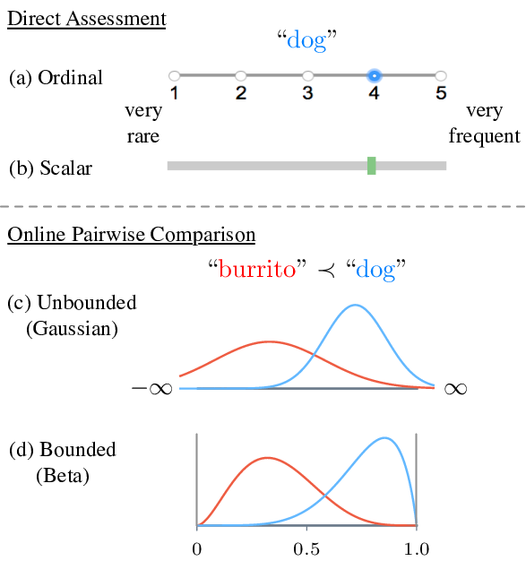
Figure 1: Elicitation strategies for graded response include direct assessment via ordinal or scalar judgments, and pairwise comparisons aggregated via an assumption of latent distributions such as Gaussians, or novel here: Beta distributions, providing bounded support. The example concerns subjective assessments of the lexical frequency of dog. In pairwise comparison, we assess it by comparison such as “burrito” is less frequent ($\prec$) than “dog”.

Many NLP datasets involve eliciting from annotators some graded response. The most popular annotation scheme is the $n$-ary ordinal approach as illustrated in Figure 1(a). For example, text may be labeled for sentiment as positive, neutral or negative (Wiebe et al., 1999; Pang et al., 2002; Turney, 2002, inter alia); or under political spectrum analysis as liberal, neutral, or conservative O’Connor et al. (2010); Bamman and Smith (2015). A response may correspond to a likelihood judgment, e.g., how likely a predicate is factive Lee et al. (2015), or that some natural language inference may hold Zhang et al. (2017). Responses may correspond to a notion of semantic similarity, e.g., whether one word can be substituted for another in context Pavlick et al. (2015), or whether an entire sentence is more or less similar than another Marelli et al. (2014), and so on.

Less common in NLP are system comparisons based on direct human ratings, but an exception includes the annual shared task evaluations of the Conference on Machine Translation (WMT). There, MT practitioners submit system outputs based on a shared set of source sentences, which are then judged relative to other system outputs. Various aggregation strategies have been employed over the years to take these relative comparisons and derive competitive rankings between shared task entrants Callison-Burch et al. (2012); Bojar et al. (2013, 2014, 2015, 2016, 2017).

Inspired by prior work in MT system evaluation, we propose a procedure for eliciting graded responses that we demonstrate to be more efficient than prior work. While remaining applicable to system evaluation, our experimental results suggest our approach as a more general framework for a variety of future data creation tasks, allowing for higher quality data in less time and cost.

We consider three different approaches for scalar annotation: direct assessment (DA), online pairwise ranking aggregation (RA), and a hybrid method which we call EASL (Efficient Annotation of Scalar Labels). DA scalar annotation, shown in Figure 1(b), directly annotates absolute judgments on some scale (e.g., 0 to 100), independently per item (§2). As an RA approach (§3), we start with conventional unbounded models, where each instance is parameterized as a Gaussian distribution, as shown in Figure 1(c). Since boundedness is essential for the scalar annotation we aim to model, we propose a bounded variant which parameterizes each instance by a beta distribution as illustrated in Figure 1(d). Finally, we propose EASL (§4) that combines benefits of DA and RA.

We illustrate the improvements enabled by our proposal on three example tasks (§5): lexical frequency inference, political spectrum inference and machine translation system ranking. For example, we find that in the commonly employed condition of 3-way redundant annotation, our approach on multiple tasks gives similar quality with just 2-way redundancy: this translates to a potential 50% increase in dataset size for the same cost.

2 Direct Assessment

Direct assessment or direct annotation (DA) is a straightforward method for collecting graded response from annotators. The most popular scheme is $n$-ary ordinal labeling, as illustrated in Figure 1(a), where annotators are shown one instance (i.e., sample point) and asked to label one of the $n$-ary ordered classes.

According to the level of measurement in psychometrics (Stevens, 1946, inter alia), which classifies the numerals based on certain properties (e.g., identity, order, quantity), ordinal data do not allow for degree of difference. Namely, there is no guarantee that the distance between each label is equal, and instances in the same class are not discriminated. For example, in a typical five-level Likert scale Likert (1932) of likelihood – very unlikely, unlikely, unsure, likely, very likely – we cannot conclude that very likely instances are exactly twice as likely those marked likely, nor can we assume two instances with the same label have exactly the same likelihood.

The issue of distance between ordinals is perhaps obviated by using scalar annotations (i.e., ratio scale in Stevens’s terminology), which directly correspond to continuous quantities (Figure 1(b)). In scalar DA, each instance in the collection ($S_{i}\in S_{1}^{N}$) is annotated with values (e.g., on the range 0 to 100) often by several annotators. The notion of quantitative difference is enabled by the property of absolute zero: the scale is bounded. For example, distance, length, mass, size etc. are represented by this scale. In the annual shared task evaluation of the WMT, DA has been used for scoring adequacy and fluency of machine learning system outputs with human evaluation Graham et al. (2013, 2014); Bojar et al. (2016, 2017), and has separately been used in creating datasets such as for factuality Lee et al. (2015).

Why perhaps obviated? Because of two concerns: (1) annotators may not have a pre-existing, well-calibrated scale for performing DA on a particular collection according to a particular task; and (2) it is known that people may be biased in their scalar estimates Tversky and Kahneman (1974). Regarding (1), this motivates us to consider RA on the intuition that annotators may give more calibrated responses when performed in the context of other elements. Regarding (2), our goal is not to correct for human bias, but simply to more efficiently converge to the same consensus judgments already being pursued by the community in their annotation protocols, biased or otherwise.

3 Online Pairwise Ranking Aggregation

3.1 Unbounded Model

Pairwise ranking aggregation Thurstone (1927) is a method to obtain a total ranking on instances, assuming that scalar value for each sample point follows a Gaussian distribution, $\mathcal{N}(\mu_{i},\sigma^{2})$. The parameters {$\mu_{i}$} are interpreted as mean scalar annotation.

Given the parameters, the probability that $S_{i}$ is preferred ($\succ$) over $S_{j}$ is defined as

$$p(S_{i}\succ S_{j}) =\Phi\left(\frac{\mu_{i}-\mu_{j}}{\sqrt{2}\sigma}\right),$$ (1)

where $\Phi(\cdot)$ is the cumulative distribution function of the standard normal distribution. The objective of pairwise ranking aggregation (including all the following models) is formulated as a maximum log-likelihood estimation:

$$\max_{\{S_{1}^{N}\}}\sum_{S_{i},S_{j}\in\{S_{1}^{N}\}}\log p(S_{i}\succ S_{j}).$$ (2)

TrueSkill^TM Herbrich et al. (2006) extends the Thurstone model by applying a Bayesian online and active learning framework, allowing for ties. TrueSkill has been used in the Xbox Live online gaming community, and has been applied for various NLP tasks, such as question difficulty estimation Liu et al. (2013), ranking speech quality Baumann (2017), and ranking machine translation and grammatical error correction systems with human evaluation Bojar et al. (2014, 2015); Sakaguchi et al. (2014, 2016)

22

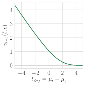
(a) $v_{i\succ j}$

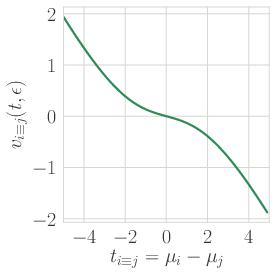
(b) $v_{i\equiv j}$

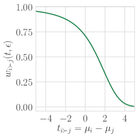
(c) $w_{i\succ j}$

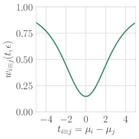
(d) $w_{i\equiv j}$

Figure 2: Surprisal of the outcome for $\mu$ and $\sigma^{2}$ ($\epsilon=0.5)$.

In the same way as the Thurstone model, TrueSkill assumes that scalar values for each instance $S_{i}$ (i.e., skill level for each player in the context of TrueSkill) follow a Gaussian distribution $\mathcal{N}(\mu_{i},\sigma^{2}_{i})$, where $\sigma_{i}$ is also parameterized as the uncertainty of the scalar value for each instance. Importantly, TrueSkill uses a Bayesian online learning scheme, and the parameters are iteratively updated after each observation of pairwise comparison (i.e., game result: win ($\succ$), tie ($\equiv$), or loss ($\prec$)) in proportion to how surprising the outcome is. Let $t_{i\succ j}=\mu_{i}-\mu_{j}$, the difference in scalar responses (skill levels) when we observe $i$ wins $j$, and $\epsilon\geqslant 0$ be a parameter to specify the tie rate. The update functions are formulated as follows:

$$\mu_{i} =\mu_{i}+\frac{\sigma^{2}_{i}}{c}\cdot v\left(\frac{t}{c},\frac{\epsilon}{c}\right)$$ (3)

$$\mu_{j} =\mu_{j}-\frac{\sigma^{2}_{j}}{c}\cdot v\left(\frac{t}{c},\frac{\epsilon}{c}\right),$$ (4)

where $c^{2}=2\gamma^{2}+\sigma^{2}_{i}+\sigma^{2}_{j}$, and $v$ are multiplicative factors that affect the amount of change (surprisal of the outcome) in $\mu$. In the accumulation of the variances ($c^{2}$), another free parameter called “skill chain”, $\gamma$, indicates the width (or difference) of skill levels that two given players have 0.8 (80%) probability of win/lose. The multiplicative factor depends on the observation (wins or ties):

$$v_{i\succ j}(t,\epsilon) =\frac{\varphi(-\epsilon+t)}{\Phi(-\epsilon+t)},$$ (5)

$$v_{i\equiv j}(t,\epsilon) =\frac{\varphi(-\epsilon-t)-\varphi(\epsilon-t)}{\Phi(\epsilon-t)-\Phi(-\epsilon-t)},$$ (6)

where $\varphi(\cdot)$ is the probability density function of the standard normal distribution. As shown in Figure 2 (a) and (b), $v_{i\succ j}$ increases exponentially as $t$ becomes smaller (i.e., the observation is unexpected), whereas $v_{i\equiv j}$ becomes close to zero when $|t|$ is close to zero. In short, $v$ becomes larger as the outcome is more surprising.

In order to update variance ($\sigma^{2}$), another set of update functions is used:

$$\sigma^{2}_{i} =\sigma^{2}_{i}\cdot\left[1-\frac{\sigma^{2}_{i}}{c^{2}}\cdot w\left(\frac{t}{c},\frac{\epsilon}{c}\right)\right]$$ (7)

$$\sigma^{2}_{j} =\sigma^{2}_{j}\cdot\left[1-\frac{\sigma^{2}_{j}}{c^{2}}\cdot w\left(\frac{t}{c},\frac{\epsilon}{c}\right)\right],$$ (8)

where $w$ serve as multiplicative factors that affect the amount of change in $\sigma^{2}$.

$$w_{i\succ j}(t,\epsilon) =v_{i\succ j}\cdot\left(v_{i\succ j}+t-\epsilon\right)$$ (9)

$$w_{i\equiv j}(t,\epsilon) =v_{i\equiv j}^{2}+\frac{(\epsilon-t)\cdot\varphi(\epsilon-t)+(\epsilon+t)\cdot\varphi(\epsilon+t)}{\Phi(\epsilon-t)-\Phi(-\epsilon-t)}.$$ (10)

As shown in Figure 2 (c) and (d), the value of $w$ is between 0 and 1. The underlying idea for the variance updates is that these updates always decrease the size of the variances $\sigma^{2}$, which means uncertainty of the instances ($S_{i},S_{j}$) always decreases as we observe more pairwise comparisons. In other words, TrueSkill becomes more confident in the current estimate of $\mu_{i}$ and $\mu_{j}$. Further details are provided by Herbrich et al. (2006).

Another important property of TrueSkill is “match quality (chance to draw)”. The match quality helps selecting competitive players to make games more interesting. More broadly, the match quality enables us to choose similar instances to be compared to maximize the information gain from pairwise comparisons, as in the active learning literature Settles et al. (2008). The match quality between two instances (players) is computed as follows:

$$q(\gamma,S_{i},S_{j}):=\sqrt[]{\frac{2\gamma^{2}}{c^{2}}}\exp{\left(-\frac{(\mu_{i}-\mu_{j})^{2}}{2c^{2}}\right)}$$ (11)

Intuitively, the match quality is based on the difference $\mu_{i}-\mu_{j}$. As the difference becomes smaller, the match quality goes higher, and vice versa.

As mentioned, TrueSkill has been used for NLP tasks to infer continuous values for instances. However, it is important to note that the support of a Gaussian distribution is unbounded, namely $\mathbb{R}=(-\infty,\infty)$. This does not satisfy the property of absolute zero of scalar annotation in the level of measurement (§2). It becomes problematic when it comes to annotating a scalar (continuous) value for extremes such as extremely positive or negative sentiments. We address this issue by proposing a novel variant of TrueSkill in the next section.

3.2 Bounded Variant

TrueSkill can induce a continuous spectrum of instances (such as skill level of game players) by assuming that each instance is represented as a Gaussian distribution. However, the Gaussian distribution has unbounded support, namely $\mathbb{R}=(-\infty,\infty)$, which does not satisfy the property of absolute bounds for appropriate scalar annotation (i.e., ratio scale in the level of measurement).

Thus, we propose a variant of TrueSkill by changing the latent distribution from a Gaussian to a beta, using a heuristic algorithm based on TrueSkill for inference. The Beta distribution has natural $[0,1]$ upper and lower bounds and a simple parameterization: $S_{i}\sim\mathcal{B}_{i}(\alpha_{i},\beta_{i})$. We choose the scalar response as the mode $\mathbb{M}[S_{i}]$ of the distribution and the variance as uncertainty:

$$\mathbb{M}_{i} =\frac{\alpha_{i}-1}{\alpha_{i}+\beta_{i}-2}$$ (12)

$$\text{Var}_{i} =\sigma^{2}_{i}=\frac{\alpha_{i}\beta_{i}}{(\alpha_{i}+\beta_{i})^{2}(\alpha_{i}+\beta_{i}+1)}$$ (13)

As in TrueSkill, we iteratively update parameters of instances $\mathcal{B}(\alpha,\beta)$ according to each observation and how it is surprising. Similarly to Eqns. (3) and (4), we choose the update functions as follows; first, in case that an annotator judged that $S_{i}$ is preferred to $S_{j}$ ($S_{i}\succ S_{j}$),

$$\alpha_{i}=\alpha_{i}+\frac{\sigma^{2}_{i}}{c}\cdot(1-p_{i\succ j})$$ (14)

$$\beta_{j}=\beta_{j}+\frac{\sigma^{2}_{j}}{c}\cdot(1-p_{j\prec i})$$ (15)

in case of ties with $|D|>\epsilon$ and $\mathbb{M}_{i}>\mathbb{M}_{j}$,

$$\alpha_{j}=\alpha_{j}+\frac{\sigma^{2}_{j}}{c}\cdot(1-p_{i\equiv j})$$ (16)

$$\beta_{i}=\beta_{i}+\frac{\sigma^{2}_{i}}{c}\cdot(1-p_{i\equiv j})$$ (17)

and in case of ties with $|D|\leqslant\epsilon$, for both $S_{i},S_{j}$,

$$\alpha_{i,j}=\alpha_{i,j}+\frac{\sigma^{2}_{i,j}}{c}\cdot(1-p_{i\equiv j})$$ (18)

$$\beta_{i,j}=\beta_{i,j}+\frac{\sigma^{2}_{i,j}}{c}\cdot(1-p_{i\equiv j}).$$ (19)

Regarding the probability of pairwise comparison between instances, we follow Bradley and Terry (1952) and Rao and Kupper (1967) to describe the chance of win, tie, or loss, as follows:

$$p(S_{i}\succ S_{j})=p(D>\epsilon)=\frac{\pi_{i}}{\pi_{i}+\theta\pi_{j}}$$ (20)

$$p(S_{i}\prec S_{j})=p(D<-\epsilon)=\frac{\pi_{j}}{\theta\pi_{i}+\pi_{j}}$$ (21)

$$p(S_{i}\equiv S_{j})=p(|D|\leqslant\epsilon)=\frac{(\theta^{2}-1)\pi_{i}\pi_{j}}{(\pi_{i}+\theta\pi_{j})(\theta\pi_{i}+\pi_{j})}$$ (22)

where $D=\mathbb{M}_{i}-\mathbb{M}_{j}$, $\epsilon\geqslant 0$ is a parameter to specify the tie rate, $\theta=\exp{(\epsilon)}$, and $\pi$ is an exponential score function of $S$; $\pi_{i}=\exp(\mathbb{M}_{i})$.

12

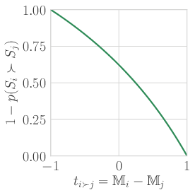
(a) $1-p_{i\succ j}$

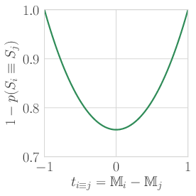
(b) $1-p_{i\equiv j}$

Figure 3: Surprisal of the outcome for the bounded variant ($\epsilon=0.5)$.

It is important to note that $\alpha$ and $\beta$ never decrease (because $1-p\geq 0$ as shown Figure 3), which satisfies the property that variance (uncertainty) always decreases as we observe more judgments, as seen in TrueSkill (§3.1). In addition, we do not need individual update functions for $\mu$ and $\sigma^{2}$, since the mode and variance in beta distribution depend on two shared parameters $\alpha,\beta$ (Eqns. 12 and 13).

Regarding match quality, we use the same formulation as the TrueSkill (Eqn. 11), except that the bounded model uses $\mathbb{M}$ instead of $\mu$:

$$q(\gamma,S_{i},S_{j})=\sqrt[]{\frac{2\gamma^{2}}{c^{2}}}\exp{\left(-\frac{(\mathbb{M}_{i}-\mathbb{M}_{j})^{2}}{2c^{2}}\right)}$$ (23)

4 Efficient Annotation of Scalar Labels

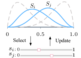
Figure 4: Illustrative example of the EASL protocol. Each instance is represented as a beta distribution. Instances are chosen to annotate according to the variance and match quality, and the parameters are updated iteratively.

In the previous section, we propose a bounded online ranking aggregation model for scalar annotation. However, the amount of update by a pairwise judgment depends only on the distance between instances, not on the distance from the bounds (i.e., 0 and 1). To integrate this property into the online ranking aggregation model, we propose EASL (Efficient Annotation of Scalar Labels) that combines benefits from both direct assessment (DA) and bounded online ranking aggregation model (RA).

Similarly to RA, EASL parameterizes each instance by a beta distribution (Eqns. 12 and  13), and the parameters are inferred using a computationally efficient and easy-to-implement heuristic. The difference from RA is the type of annotation. While we ask for discrete pairwise judgment ($\succ,\prec,\equiv$) between $S_{i}$ and $S_{j}$ in RA, here we directly ask for scalar values for them (denoted as $s_{i}$ and $s_{j}$) as in DA. Thus, given an annotated score $s_{i}$ which is normalized between [0,1], we change the update functions as follows:

$$\alpha_{i} =\alpha_{i}+s_{i}$$ (24)

$$\beta_{i} =\beta_{i}+(1-s_{i})$$ (25)

This procedure may look similar to DA, where $s_{i}$ is simply accumulated and averaged at the end. However, there are two differences. First, as illustrated in Figure 4, EASL parameterizes each instance as a probability distribution while DA does not. Second, DA elicits annotations independently per element, whereas EASL elicits annotations on elements in the context of other elements selected jointly according to match quality.

Further, DA generally uses a batch style annotation scheme, where the number of annotations per instance is independent from the latent scalar values. On the other hand, EASL uses online learning, which impacts the calculation of match quality. This allows us to choose instances to annotate by order of uncertainty for each instance, and as in RA, the match quality (Eqn. 23) enables us to consider similar instances in the same context.

5 Experiments

To compare different annotation methods, we conduct three experiments: (1) lexical frequency inference, (2) political spectrum inference, and (3) human evaluation for machine translation systems.

In all experiments, data collection is conducted through Amazon Mechanical Turk (AMT). We ask annotators who meet the following minimum requirements: living in the US, overall approval rate $>$ 98%, and number of tasks approved $>$ 500.

The experimental setting for DA is straightforward. We ask annotators to annotate a scalar value for each instance, one item at a time. We collect ten annotations for each instance to see the relation between the number of annotations and accuracy (i.e., correlation).

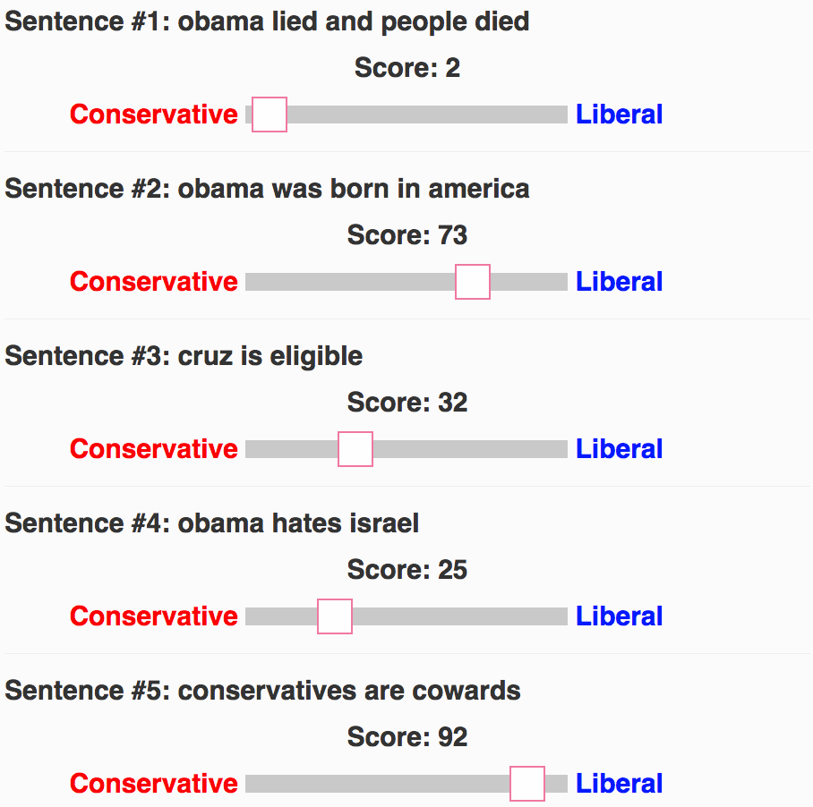
Figure 5: Example of partial ranking with scalars (HITS)

To set up the online update in RA and EASL, we use a partial ranking framework with scalars, where annotators are asked to rank and score $n$ instances at one time as illustrated in Figure 5. In all three experiments, we fix $n=5$. The partial ranking yields $\binom{n}{2}$ pairwise comparisons for RA and $n$ scalar values for EASL. It is important to note that we can simultaneously retrieve pairwise judgments ($\succ,\prec,\equiv$) as well as scalar values from this format.

Input: Instances $\{S_{1}^{N}\}$

Output: Updated instances $\{S_{1}^{N}\}$

/* Initialize params */

1 $(\alpha_{i},\beta_{i})_{\in S}=(\alpha_{i}^{\text{init}},\beta_{i}^{\text{init}})$

/* Update $S$ over iterations */

2 foreach iteration do

3      HITS = SampleByMatchQuality($S,N,n$)

4      $A$ = Annotate(HITS)

5      for obs $\in A$ do // Update $S$

6           $i,j,d$ = parseObservation($obs$)

7           $\alpha_{i,j},\beta_{i,j}$ = update($i,j,d$)

8          

9          

10           return $S$

11           Function SampleByMatchQuality($S,N,n$)

12                $k=N/n$

13                descendingSort($S$, key=Var[$S$])

14                $S^{\prime}=$ top-k instances of $S$

15                HITS = []

16                foreach $S_{i}\in S^{\prime}$ do

17                     m = []

18                     foreach $S_{j}\in S_{/S^{\prime}}$ do

19                          m.append([matchQuality($S_{i},S_{j}$), $j$])

20                         

21                          $p$ = normalize(m)

22                          $\tilde{S}$ = sampling n-1 items by $p$

23                          HITS.append([$S_{i},\tilde{S}$])

24                         

25                          return HITS

26                         

Algorithm 1 Online pairwise ranking aggregation with bounded support.

In each iteration, $n$ instances are selected by variance and match quality. We first select top k ($=N/n$) instances according to the variance, and for each selected instance we choose the other $n-1$ instances to be compared based on match quality. This approach has been used in the NLP community in tasks such as for assessing machine translation quality Bojar et al. (2014); Sakaguchi et al. (2014); Bojar et al. (2015, 2016) to collect pairwise judgments efficiently. The detailed procedure of iterative parameter updates in the RA and EASL is described in Algorithm 1. As mentioned in Section 4, the main difference between RA and EASL is the update functions (line 7).

Model hyper-parameters in RA and EASL are set as follows; each instance is initialized as $\alpha_{i}^{\text{init}}=1.0$, $\beta_{i}^{\text{init}}=1.0$. The skill chain parameter $\gamma$ and tie-rate parameter $\epsilon$ are set to be 0.1.

5.1 Lexical Frequency Inference

In the first experiment, we compare the three scalar annotation approaches on lexical frequency inference, in which we ask annotators to judge frequency (from very rare to very frequent) of verbs that are randomly selected from the corpus of Contemporary American English (COCA). We include this task for evaluation owing to its non-subjective ground truth (relative corpus frequency) which can be used as an oracle response we would like to maximally correlate with.

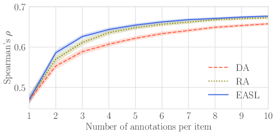
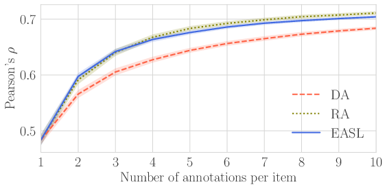
Figure 6: Spearman’s (top) and Pearson’s (bottom) correlations with three difference methods on lexical frequency inference annotation: direct assessment (DA), online ranking aggregation (RA), and EASL. The shade for each line indicates 95% confidence intervals by bootstrap resampling (running 100 times).

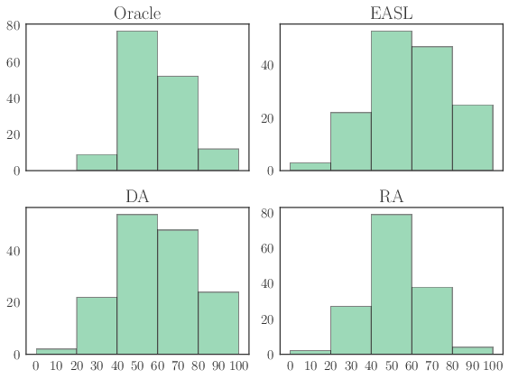
Figure 7: Histograms of scalar values on lexical frequency obtained by each annotation scheme (direct assessment (DA), online ranking aggregation (RA), and EASL), and the oracle. The scalar annotations are put into five bins to see the overall distribution. The scalar in the oracle is normalized as $log_{10}$(frequency($S_{i}$)) / $\max log_{10}$(frequency($S$)).

We randomly select 150 verbs from COCA; the log frequency ($\log_{10}$) is regarded as the oracle. In DA, each instance is annotated by 10 different annotators. In the RA and EASL, annotators are asked to rank/score five verbs for each HIT ($n=5$). Each iteration contains 20 HITS and we run 10 iterations, which means that total number of annotations is the same in DA, RA, and EASL.

14

(a) Iter 0

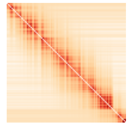
(b) Iter 3

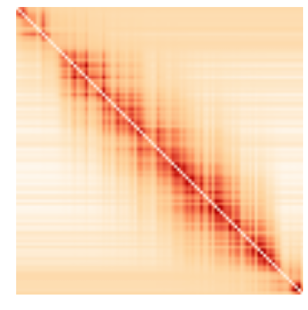
(c) Iter 6

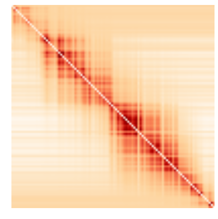
(d) Iter 9

Figure 8: Heatmaps of match quality distribution across the cross-product of instances ordered by the oracle (i.e., $log_{10}$(frequency)).

Figure 6 presents Spearman’s and Pearson’s correlations, indicating how accurately each annotation method obtains scalar values for each instance. Overall, in all three methods, the correlations are increased as more annotations are made. The result also shows that RA and EASL approaches achieve high correlation more efficiently than DA. The gain of efficiency from DA to EASL is about 50%; two iterations in EASL achieves a close Spearman’s $\rho$ to three annotators in DA.

Figure 7 presents the results of the final scalar values that each method annotated. The distribution of the histograms shows that overall three methods successfully capture the latent distribution of scalar values in the data.

Figure 8 shows a dynamic change of match quality. In the beginning (iteration 0), all the instances are equally competitive because we have no information about them and initialize them with the same parameters. As iterations go on, the instances along the diagonal have higher match quality, indicating that competitive matches are more likely to be selected for a next iteration. In other words, match-quality helps to choose informative pairs to compare at each iteration, which reduces the number of less informative annotations (e.g., a pairwise comparison between the highest and lowest instances).

5.2 Political Spectrum Inference

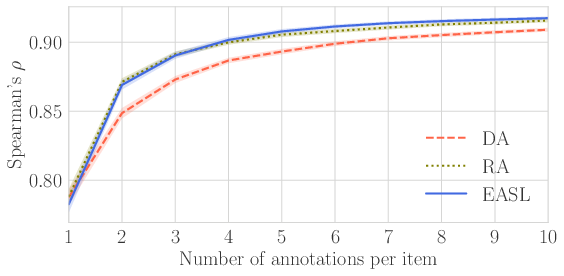
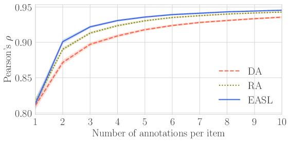
Figure 9: Spearman’s (top) and Pearson’s (bottom) correlations with three difference methods on political spectrum annotation: direct assessment (DA), online ranking aggregation (RA), and EASL

In the second experiment, we compare the three scalar annotation methods for political spectrum inference. We use the Fine-Grained Political Statements dataset Bamman and Smith (2015), which consists of 766 propositions collected from political blog comments, paired with judgments about the political belief of the statement (or the person who would say it) based on the five ordinals: very conservative (-2), slightly conservative (-1), neutral (0), slightly liberal (1), and very liberal (2). We normalize the ordinal scores between 0 and 1. The dataset contains the mean scores by aggregating 7 annotations for each proposition.

We randomly choose 150 political propositions from the dataset (see the histogram in Figure 10 oracle). The experimental setting (i.e., the number of annotations per instance, the number of iterations, and the number of HITS in each iteration) is the same as the lexical frequency inference experiment (§5.1).

Figure 9 shows Spearman’s and Pearson’s correlations to the oracle by each method. Overall, all the three methods achieve strong correlation above 0.9. We also find that RA and EASL reach high correlation more efficiently than DA as in the lexical frequency inference experiment (§5.1). The gain of efficiency from DA to EASL is about 50%; 4-way redundant annotation in EASL achieves a close Spearman’s $\rho$ to 6-way redundancy in DA.

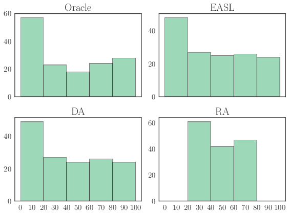
Figure 10: Histograms of scalar values on political spectrum obtained by each annotation scheme (DA, RA, EASL) and the oracle. Scalars are put into five bins to see the overall distribution.

Propositions	Gold	DA	RA	EASL
the republicans are useless	100	91.7	75.8	91.9
obama is right	92.9	90.1	74.6	90.0
hillary will win	78.6	86.3	72.9	86.4
aca is a success	75.0	78.2	68.3	77.3
harry reid is a democrat	53.6	55.5	55.8	55.9
ebola is a virus	50.0	53.0	53.8	53.5
cruz is eligible	32.2	31.0	44.0	31.4
global warming is a religion	28.6	22.4	37.3	23.0
bush kept us safe	10.7	9.6	31.5	9.6
democrats are corrupt	0.0	7.1	29.9	7.4

Table 1: Example propositions and the scalar political spectrum ranged between 0 (very conservative) and 100 (very liberal) by each approach: direct assessment, online ranking aggregation, and EASL. The dashed lines indicate a split by 5-ary ordinal scale.

Figure 10 presents the results of the annotated scalar values by each method. The distribution of the histograms shows that DA and EASL successfully fit to the distribution in the oracle, whereas RA converges to a rather narrow range. This is because of the “lack of distance from bounds” in RA that is explained in §4. We note that renormalizing the distribution in RA will not address the issue. For instance, when the dataset has only liberal propositions, RA still fails to capture the latent distribution because it looks only at relative distances between instances but not the distance from bounds. Table 1 shows the examples of scalar annotations by each method. Again, we see that RA approach has a narrower range than the oracle, DA, and EASL.

5.3 Ranking Machine Translation Systems

In the third experiment, we apply the scalar annotation methods for evaluating machine translation systems. This is different from two previous experiments, because the main purpose is to rank the MT systems ($S_{1}^{N}$) rather than the adequacy ($q$) of each MT output for a given source sentence ($m$). Namely, we want to rank $S_{i}$ by observing $q_{i,m}$.

We use WMT16 German-English translation dataset Bojar et al. (2016), which consists of 2,999 test set sentences and the translations from 10 different systems with DA annotation. Each sentence has its adequacy score annotation between 0 and 100, and the average adequacy scores are computed for each system for ranking. In this setting, annotators are asked to judge adequacy of system output(s) with the reference being given. The official scores (made by DA) and ranking in WMT16 are used as the oracle in this experiment.

In this experiment, we replicate DA and run EASL to compare the efficiency. We omit RA in this experiment, because it does not necessarily capture the distance from bounds as shown in the previous experiment (§5.2). In DA, 33,760 translation outputs (3,376 sentences per system in average) are randomly sampled without replacement to make sure that it reaches up to the same result as oracle when the entire data are used.

In EASL, we assume that adequacy ($q$) of an MT output by system ($S_{i}$) for a given source sentence ($m$) is drawn from beta distribution: $q_{i,m}\sim\mathcal{B}(\alpha_{i},\beta_{i})$. Annotators are asked to judge adequacy of system outputs by scoring 0 and 100. Similarly to the previous experiments (§ 5.1 and § 5.2), we use the partial ranking strategy, where we show $n=5$ system outputs (for the same source sentence $l$) to annotate at a time. The procedure of parameter updates is the same as previous experiments (Algorithm 1).

We compare the correlations (Spearman’s $\rho$) of system ranking with respect to the number of annotations per system, and the result is shown in Figure 11. As seen in the previous two experiments, EASL achieves higher Spearman’s correlation on ranking MT systems with smaller number of annotations than the baseline method (DA), which means EASL is able to collect annotation more efficiently. The result shows that EASL can be applied for efficient system evaluation in addition to data curation.

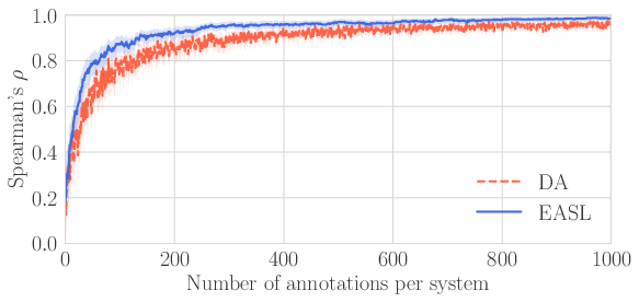
Figure 11: Spearman’s correlation on ranking machine translation systems on WMT16 German-English data: direct assessment (DA), and EASL. The shade for each line indicates 95% confidence intervals by bootstrap resampling (running 100 times).

6 Conclusions

We have presented an efficient, online model to elicit scalar annotations for computational linguistic datasets and system evaluations. The model combines two approaches for scalar annotation: direct assessment and online pairwise ranking aggregation. We conducted three illustrative experiments on lexical frequency inference, political spectrum inference, and ranking machine translation systems. We have shown that our approach, EASL (Efficient Annotation of Scalar Labels), outperforms direct assessment in terms of annotation efficiency and outperforms online ranking aggregation in terms of accurately capturing the latent distributions of scalar values. The significant gains demonstrated suggests EASL as a promising approach for future dataset curation and system evaluation in the community.

References

- Balota et al. (1999) David A. Balota, Cortese Michael J., and Maura Pilotti. 1999. Item-level analyses of lexical decision performance: Results from a mega-study. In Abstracts of the 40th Annual Meeting of the Psychonomics Society, page 44, Los Angeles, California. Psychonomic Society.
- Bamman and Smith (2015) David Bamman and Noah A. Smith. 2015. Open extraction of fine-grained political statements. In Proceedings of the 2015 Conference on Empirical Methods in Natural Language Processing, pages 76–85, Lisbon, Portugal. Association for Computational Linguistics.
- Baumann (2017) Timo Baumann. 2017. Large-scale speaker ranking from crowdsourced pairwise listener ratings. In Proceedings of Interspeech.
- Bojar et al. (2014) Ondrej Bojar, Christian Buck, Christian Federmann, Barry Haddow, Philipp Koehn, Johannes Leveling, Christof Monz, Pavel Pecina, Matt Post, Herve Saint-Amand, Radu Soricut, Lucia Specia, and Aleš Tamchyna. 2014. Findings of the 2014 workshop on statistical machine translation.
- Bojar et al. (2013) Ondřej Bojar, Christian Buck, Chris Callison-Burch, Christian Federmann, Barry Haddow, Philipp Koehn, Christof Monz, Matt Post, Radu Soricut, and Lucia Specia. 2013. Findings of the 2013 Workshop on Statistical Machine Translation. In Proceedings of the Eighth Workshop on Statistical Machine Translation, pages 1–44, Sofia, Bulgaria. Association for Computational Linguistics.
- Bojar et al. (2017) Ondřej Bojar, Rajen Chatterjee, Christian Federmann, Yvette Graham, Barry Haddow, Shujian Huang, Matthias Huck, Philipp Koehn, Qun Liu, Varvara Logacheva, Christof Monz, Matteo Negri, Matt Post, Raphael Rubino, Lucia Specia, and Marco Turchi. 2017. Findings of the 2017 conference on machine translation (wmt17). In Proceedings of the Second Conference on Machine Translation, pages 169–214, Copenhagen, Denmark. Association for Computational Linguistics.
- Bojar et al. (2016) Ondřej Bojar, Rajen Chatterjee, Christian Federmann, Yvette Graham, Barry Haddow, Matthias Huck, Antonio Jimeno Yepes, Philipp Koehn, Varvara Logacheva, Christof Monz, Matteo Negri, Aurelie Neveol, Mariana Neves, Martin Popel, Matt Post, Raphael Rubino, Carolina Scarton, Lucia Specia, Marco Turchi, Karin Verspoor, and Marcos Zampieri. 2016. Findings of the 2016 conference on machine translation. In Proceedings of the First Conference on Machine Translation, pages 131–198, Berlin, Germany. Association for Computational Linguistics.
- Bojar et al. (2015) Ondřej Bojar, Rajen Chatterjee, Christian Federmann, Barry Haddow, Matthias Huck, Chris Hokamp, Philipp Koehn, Varvara Logacheva, Christof Monz, Matteo Negri, Matt Post, Carolina Scarton, Lucia Specia, and Marco Turchi. 2015. Findings of the 2015 workshop on statistical machine translation. In Proceedings of the Tenth Workshop on Statistical Machine Translation, pages 1–46, Lisbon, Portugal. Association for Computational Linguistics.
- Bradley and Terry (1952) Ralph Allan Bradley and Milton E. Terry. 1952. Rank analysis of incomplete block designs: I. the method of paired comparisons. Biometrika, 39(3/4):324–345.
- Callison-Burch et al. (2012) Chris Callison-Burch, Philipp Koehn, Christof Monz, Matt Post, Radu Soricut, and Lucia Specia. 2012. Findings of the 2012 workshop on statistical machine translation. In Proceedings of the Seventh Workshop on Statistical Machine Translation, pages 10–51, Montréal, Canada. Association for Computational Linguistics.
- Elo (1978) Arpad E. Elo. 1978. The rating of chessplayers, past and present. Arco Pub.
- Fine et al. (2014) Alex B. Fine, Austin F. Frank, T. Florian Jaeger, and Benjamin Van Durme. 2014. Biases in predicting the human language model. In Proceedings of the 52nd Annual Meeting of the Association for Computational Linguistics (Volume 2: Short Papers), pages 7–12, Baltimore, Maryland. Association for Computational Linguistics.
- Graham et al. (2013) Yvette Graham, Timothy Baldwin, Alistair Moffat, and Justin Zobel. 2013. Continuous measurement scales in human evaluation of machine translation. In Proceedings of the 7th Linguistic Annotation Workshop and Interoperability with Discourse, pages 33–41, Sofia, Bulgaria. Association for Computational Linguistics.
- Graham et al. (2014) Yvette Graham, Timothy Baldwin, Alistair Moffat, and Justin Zobel. 2014. Is machine translation getting better over time? In Proceedings of the 14th Conference of the European Chapter of the Association for Computational Linguistics, pages 443–451, Gothenburg, Sweden. Association for Computational Linguistics.
- Herbrich et al. (2006) Ralf Herbrich, Tom Minka, and Thore Graepel. 2006. TrueSkill™: A Bayesian Skill Rating System. In Proceedings of the Twentieth Annual Conference on Neural Information Processing Systems, pages 569–576, Vancouver, British Columbia, Canada.
- Hovy et al. (2013) Dirk Hovy, Taylor Berg-Kirkpatrick, Ashish Vaswani, and Eduard Hovy. 2013. Learning whom to trust with mace. In Proceedings of the 2013 Conference of the North American Chapter of the Association for Computational Linguistics: Human Language Technologies, pages 1120–1130, Atlanta, Georgia. Association for Computational Linguistics.
- Lee et al. (2015) Kenton Lee, Yoav Artzi, Yejin Choi, and Luke Zettlemoyer. 2015. Event detection and factuality assessment with non-expert supervision. In Proceedings of the 2015 Conference on Empirical Methods in Natural Language Processing, pages 1643–1648, Lisbon, Portugal. Association for Computational Linguistics.
- Likert (1932) Rensis Likert. 1932. A technique for the measurement of attitudes. Archives of psychology.
- Liu et al. (2013) Jing Liu, Quan Wang, Chin-Yew Lin, and Hsiao-Wuen Hon. 2013. Question difficulty estimation in community question answering services. In Proceedings of the 2013 Conference on Empirical Methods in Natural Language Processing, pages 85–90, Seattle, Washington, USA. Association for Computational Linguistics.
- Marelli et al. (2014) Marco Marelli, Stefano Menini, Marco Baroni, Luisa Bentivogli, Raffaella bernardi, and Roberto Zamparelli. 2014. A sick cure for the evaluation of compositional distributional semantic models. In Proceedings of the Ninth International Conference on Language Resources and Evaluation (LREC-2014). European Language Resources Association (ELRA).
- Novikova et al. (2018) J. Novikova, O. Dušek, and V. Rieser. 2018. RankME: Reliable Human Ratings for Natural Language Generation. ArXiv e-prints.
- O’Connor et al. (2010) Brendan O’Connor, Ramnath Balasubramanyan, Bryan R Routledge, and Noah A Smith. 2010. From tweets to polls: Linking text sentiment to public opinion time series. ICWSM, 11(122-129):1–2.
- Pang et al. (2002) Bo Pang, Lillian Lee, and Shivakumar Vaithyanathan. 2002. Thumbs up?: sentiment classification using machine learning techniques. In Proceedings of the ACL-02 conference on Empirical methods in natural language processing-Volume 10, pages 79–86. Association for Computational Linguistics.
- Pavlick et al. (2015) Ellie Pavlick, Travis Wolfe, Pushpendre Rastogi, Chris Callison-Burch, Mark Dredze, and Benjamin Van Durme. 2015. Framenet+: Fast paraphrastic tripling of framenet. In Proceedings of the 53rd Annual Meeting of the Association for Computational Linguistics and the 7th International Joint Conference on Natural Language Processing (Volume 2: Short Papers), pages 408–413, Beijing, China. Association for Computational Linguistics.
- Rao and Kupper (1967) P. V. Rao and L. L. Kupper. 1967. Ties in paired-comparison experiments: A generalization of the bradley-terry model. Journal of the American Statistical Association, 62(317):194–204.
- Sakaguchi et al. (2016) Keisuke Sakaguchi, Courtney Napoles, Matt Post, and Joel Tetreault. 2016. Reassessing the goals of grammatical error correction: Fluency instead of grammaticality. Transactions of the Association for Computational Linguistics, 4:169–182.
- Sakaguchi et al. (2014) Keisuke Sakaguchi, Matt Post, and Benjamin Van Durme. 2014. Efficient elicitation of annotations for human evaluation of machine translation. In Proceedings of the Ninth Workshop on Statistical Machine Translation, pages 1–11, Baltimore, Maryland, USA. Association for Computational Linguistics.
- Settles et al. (2008) Burr Settles, Mark Craven, and Lewis Friedland. 2008. Active learning with real annotation costs. In Proceedings of the NIPS workshop on cost-sensitive learning, pages 1–10.
- Stevens (1946) S. S. Stevens. 1946. On the theory of scales of measurement. Science, 103(2684):677–680.
- Thurstone (1927) Louis L Thurstone. 1927. The method of paired comparisons for social values. The Journal of Abnormal and Social Psychology, 21(4):384.
- Turney (2002) Peter D Turney. 2002. Thumbs up or thumbs down?: semantic orientation applied to unsupervised classification of reviews. In Proceedings of the 40th annual meeting on association for computational linguistics, pages 417–424. Association for Computational Linguistics.
- Tversky and Kahneman (1974) Amos Tversky and Daniel Kahneman. 1974. Judgment under uncertainty: Heuristics and biases. Science, 185(4157):1124–1131.
- Welinder et al. (2010) Peter Welinder, Steve Branson, Pietro Perona, and Serge J Belongie. 2010. The multidimensional wisdom of crowds. In Advances in neural information processing systems, pages 2424–2432.
- Whitehill et al. (2009) Jacob Whitehill, Ting-fan Wu, Jacob Bergsma, Javier R Movellan, and Paul L Ruvolo. 2009. Whose vote should count more: Optimal integration of labels from labelers of unknown expertise. In Advances in neural information processing systems, pages 2035–2043.
- Wiebe et al. (1999) Janyce M Wiebe, Rebecca F Bruce, and Thomas P O’Hara. 1999. Development and use of a gold-standard data set for subjectivity classifications. In Proceedings of the 37th annual meeting of the Association for Computational Linguistics on Computational Linguistics, pages 246–253. Association for Computational Linguistics.
- Zhang et al. (2017) Sheng Zhang, Rachel Rudinger, Kevin Duh, and Benjamin Van Durme. 2017. Ordinal common-sense inference. Transactions of the Association for Computational Linguistics, 5:379–395.