$\chi_{\textrm{top}}(T\gg T_{\mathrm{c}})$ in pure-glue QCD through reweighting

Abstract

We calculate the topological susceptibility at $2.5~{}T_{\mathrm{c}}$ and $4.1~{}T_{\mathrm{c}}$ in SU(3) pure Yang-Mills theory. We define topology with the help of gradient flow and we largely overcome the problem of poor statistics at high temperatures by applying a reweighting technique in terms of the topological charge, measured after a specific small amount of gradient flow. This allows us to obtain a sample of configurations which compares topological sectors with good statistics, with enhanced tunneling between topologies. We quote continuum extrapolated results at these two temperatures and conclude that our method is viable and can be extended without new conceptual problems to the case of full QCD with fermions.

I Introduction

Two of the most challenging problems in particle physics are the strong CP problem and the origin of dark matter. The axion Weinberg (1978); Wilczek (1978), a hypothetical light scalar particle which appears in the Peccei-Quinn mechanism Peccei and Quinn (1977a, b), could solve both problems at once: The additional degrees of freedom explain that the CP violating phase $\Theta_{\mathrm{QCD}}$ in the QCD Lagrangian vanishes Peccei and Quinn (1977b) and the corresponding particle could play the role of dark matter in the Universe Preskill et al. (1983); Abbott and Sikivie (1983); Dine and Fischler (1983).

There is currently a lot of experimental effort to detect axions; for a review on this we refer to Ref. Irastorza and Redondo (2018). From a theory point of view, the properties of the axion are sensitive to the topological susceptibility of QCD $\chi(T)$, defined as

$$\chi(T)=\int\mathrm{d}^{4}x\mathopen{}\mathclose{{}\left\langle q(x)q(0)}\right\rangle_{\beta}=\frac{1}{\beta V}\mathopen{}\mathclose{{}\left\langle Q^{2}}\right\rangle,$$ (1)

with $q(x)$ the topological charge density and $Q=\int\mathrm{d}^{4}x\;q(x)$ its integral (defined below). While the topological susceptibility at low temperatures is well established Grilli di Cortona et al. (2016), calculations become much more challenging at high temperatures, and axion cosmology requires knowledge of $\chi(T)$ at temperatures up to about $7~{}T_{\mathrm{c}}$ Moore (2018); Klaer and Moore (2017). Recently there has been a burst of progress in determining $\chi(T)$ at high temperatures Frison et al. (2016); Berkowitz et al. (2015); Taniguchi et al. (2017); Bonati et al. (2016); Petreczky et al. (2016); Borsanyi et al. (2016a, b). However, we feel that it would still be valuable to make an independent study of topological susceptibility which reaches up to 7 $T_{\mathrm{c}}$.

At high temperatures topology is expected to be dominated by rare single instanton Belavin et al. (1975); ’t Hooft (1976) (really caloron Harrington and Shepard (1978)) configurations with a typical size $\rho\sim 0.4/T$ Gross et al. (1981). These configurations become more suppressed as one considers higher temperatures, by $\chi(T)\propto T^{-7}$ (at lowest perturbative order in pure-glue gauge theory; with light fermions there is an additional factor of $T^{-N_{\mathrm{f}}/3}$). This makes studying topology by lattice Monte Carlo simulations challenging; in an ensemble of high-temperature gauge theory configurations, virtually none of the configurations will possess topology, leading to severely limited statistics. For instance, if we keep the number of temporal points across the lattice fixed, the instanton density in terms of lattice sites vanishes as $T^{-11}$. Furthermore, the efficiency with which a Markov chain algorithm samples these topological configurations will be additionally suppressed, because the chain must pass through “small” instantons (or dislocations) to move between distinct topological sectors, and these dislocations get rarer with decreasing lattice spacing as $a^{-11}$.

One way around this problem is to measure topology at a low temperature where instantons are not rare, and to work up to high temperatures differentially by studying fixed-topology ensembles Borsanyi et al. (2016b); Frison et al. (2016). But we feel it is important as a cross-check to be able to perform a direct study of topology at high temperature. This will require a reweighting procedure to overcome the sampling challenges. Our goal in this paper is to present such a reweighting approach. Since this work is exploratory, we will content ourselves with a study of the quenched (or pure-glue) theory. Once the technique is well established, we see no obstacles in adapting it to the unquenched case (though there will be the usual increase in numerical cost associated with going from pure glue to unquenched).

This paper is organized as follows: In Sec. II, we discuss in detail the method that we use to enhance the number of instantons in the lattice simulations, namely a combination of gradient flow and reweighting. Results of the topological susceptibility of the quenched theory up to $4.1~{}T_{\mathrm{c}}$ obtained with this method are presented in Sec. III. Conclusions and a discussion can then be found in Sec. IV.

II Method

The statistical problem of calculating the topological susceptibility at high temperatures on the lattice is twofold. First, the quantity is expected to be physically very small which will result in most of the configurations having $Q=0$. Only by collecting a huge amount of statistics, a meaningful statement about expectation values involving the topological charge can be made. This problem becomes more severe as one goes to higher temperatures. And in addition, the algorithm itself used to generate the sample (usually heatbath/overrelaxation or HMC) tends to get stuck in the different topological sectors, with tunneling events between sectors more and more suppressed as one takes the continuum limit. Here we show how to use reweighting to overcome both problems.

II.1 Definition of reweighting

Our reweighting approach is an evolution of those in Refs. Berg and Neuhaus (1991); Kajantie et al. (1996); Laine and Rummukainen (1998); Wang and Landau (2001). Since the topological charge is not restricted to integer values on the lattice, rare events exist that will enable tunneling between different sectors. The goal is then to enhance those and use them to generate a sample of configurations almost homogeneously distributed across the topological sectors of interest. At the same time, it is mandatory to be able to know by how much they were enhanced so that this effect can be removed at the end without losing the statistical power. In the following, we describe one way of achieving this for the case of pure SU(3) Yang-Mills theory with periodic boundary conditions.

The nonperturbative approach of lattice gauge theory is based on a stochastic evaluation of the partition function

$$\mathcal{Z}=\int\mathcal{D}U\mathrm{e}^{-S_{\mathrm{W}}[U]}.$$ (2)

Here $S_{\mathrm{W}}[U]$ is the ordinary SU(3) plaquette Wilson action and $U$ are the links. The algorithmic challenge consists in obtaining a sample of configurations which is precisely distributed according to the probability distribution

$$\mathrm{d}P(U)=\frac{1}{\mathcal{Z}}\mathrm{\mathrm{e}}^{-S_{\mathrm{W}}[U]}\mathrm{d}U.$$ (3)

In this way, importance sampling enables the calculation of expectation values of gauge invariant operators via the simple mean

$$\langle O\rangle=\frac{1}{N}\sum^{N}_{i}\mathcal{O}_{i}.$$ (4)

At high temperatures well above $T_{\mathrm{c}}$, the ordinary approach just described will yield an ensemble with very little topological information. Reweighting works by rewriting Eq. (2) as

$$\mathcal{Z}=\int\mathcal{D}U\mathrm{e}^{-S_{\mathrm{W}}[U]+W(\xi)}\mathrm{e}^{-W(\xi)},$$ (5)

and therefore, Eq. (4) turns into

$$\langle\mathcal{O}\rangle=\frac{\sum^{N}_{i}\mathcal{O}_{i}\mathrm{e}^{-W(\xi_{i})}}{\sum^{N}_{i}\mathrm{e}^{-W(\xi_{i})}}$$ (6)

if the ensemble is distributed according to the modified probability distribution

$$\mathrm{d}P_{\mathrm{rew}}(U)=\frac{\mathrm{e}^{-S_{\mathrm{W}}[U]+W(\xi)}\mathrm{d}U}{\int\mathcal{D}U\mathrm{e}^{-S_{\mathrm{W}}[U]+W(\xi)}}.$$ (7)

Notice that it is guaranteed that Eqs. (4) and (6) yield identical results for any choice of the reweighting function $W$ as long as our algorithm converges to Eq. (7) and $N\to\infty$. The argument $\xi$ is an arbitrary set of reweighting variables which need to be measured on each produced configuration.

II.2 Choice of reweighting variable

If chosen correctly, reweighting variables can account for a clear distinction between different phases and therefore favor or suppress certain sectors in Monte Carlo space. A natural choice is then the topological charge itself:

$$Q=\sum_{x}q(x)=\frac{1}{64\pi^{2}}\epsilon_{\mu\nu\rho\sigma}\sum_{x}\hat{F}_{\mu\nu}^{a}(x)\hat{F}_{\rho\sigma}^{a}(x).$$ (8)

Here $\hat{F}_{\mu\nu}(x)$ is a lattice discretized form of the field strength. The conventional choice is the “clover” value (the average over the four square plaquettes touching the point $x$), but we use an $a^{2}$-improved choice composed of a linear combination of squares and $1\times 2$ rectangles Jahn et al. (2018), specifically

$$\begin{split}\hat{F}_{\mathrm{clov}}&=\frac{1}{4}\begin{picture}(25.0,20.0)\put(4.0,-4.0){\line(1,0){16.0}}\put(4.0,4.0){\line(1,0){16.0}}\put(4.0,12.0){\line(1,0){16.0}} \put(4.0,-4.0){\line(0,1){16.0}}\put(12.0,-4.0){\line(0,1){16.0}}\put(20.0,-4.0){\line(0,1){16.0}} \put(12.0,4.0){\circle*{4.0}} \end{picture}\\ \hat{F}_{\mathrm{imp}}&=\frac{5}{12}\begin{picture}(25.0,20.0)\put(4.0,-4.0){\line(1,0){16.0}}\put(4.0,4.0){\line(1,0){16.0}}\put(4.0,12.0){\line(1,0){16.0}} \put(4.0,-4.0){\line(0,1){16.0}}\put(12.0,-4.0){\line(0,1){16.0}}\put(20.0,-4.0){\line(0,1){16.0}} \put(12.0,4.0){\circle*{4.0}} \end{picture}-\frac{1}{24}\mathopen{}\mathclose{{}\left(\begin{picture}(40.0,20.0)\put(4.0,-4.0){\line(1,0){32.0}}\put(4.0,4.0){\line(1,0){32.0}}\put(4.0,12.0){\line(1,0){32.0}} \put(4.0,-4.0){\line(0,1){16.0}}\put(20.0,-4.0){\line(0,1){16.0}}\put(36.0,-4.0){\line(0,1){16.0}} \put(12.0,-4.0){\put(0.0,0.0){\line(0,1){1.0}}\put(0.0,2.0){\line(0,1){1.0}}\put(0.0,4.0){\line(0,1){1.0}}\put(0.0,6.0){\line(0,1){1.0}}\put(0.0,8.0){\line(0,1){1.0}}\put(0.0,10.0){\line(0,1){1.0}}\put(0.0,12.0){\line(0,1){1.0}}\put(0.0,14.0){\line(0,1){1.0}}}\put(28.0,-4.0){\put(0.0,0.0){\line(0,1){1.0}}\put(0.0,2.0){\line(0,1){1.0}}\put(0.0,4.0){\line(0,1){1.0}}\put(0.0,6.0){\line(0,1){1.0}}\put(0.0,8.0){\line(0,1){1.0}}\put(0.0,10.0){\line(0,1){1.0}}\put(0.0,12.0){\line(0,1){1.0}}\put(0.0,14.0){\line(0,1){1.0}}} \put(20.0,4.0){\circle*{4.0}} \end{picture}+\begin{picture}(25.0,22.0)\put(4.0,-12.0){\line(1,0){16.0}}\put(4.0,4.0){\line(1,0){16.0}}\put(4.0,20.0){\line(1,0){16.0}} \put(4.0,-12.0){\line(0,1){32.0}}\put(12.0,-12.0){\line(0,1){32.0}}\put(20.0,-12.0){\line(0,1){32.0}} \put(4.0,-4.0){\put(0.0,0.0){\line(1,0){1.0}}\put(2.0,0.0){\line(1,0){1.0}}\put(4.0,0.0){\line(1,0){1.0}}\put(6.0,0.0){\line(1,0){1.0}}\put(8.0,0.0){\line(1,0){1.0}}\put(10.0,0.0){\line(1,0){1.0}}\put(12.0,0.0){\line(1,0){1.0}}\put(14.0,0.0){\line(1,0){1.0}}}\put(4.0,12.0){\put(0.0,0.0){\line(1,0){1.0}}\put(2.0,0.0){\line(1,0){1.0}}\put(4.0,0.0){\line(1,0){1.0}}\put(6.0,0.0){\line(1,0){1.0}}\put(8.0,0.0){\line(1,0){1.0}}\put(10.0,0.0){\line(1,0){1.0}}\put(12.0,0.0){\line(1,0){1.0}}\put(14.0,0.0){\line(1,0){1.0}}} \put(12.0,4.0){\circle*{4.0}} \end{picture}}\right).\end{split}$$ (9)

However, using $Q$ directly on the original configuration actually fails, because the topological density contains high-dimension operator corrections which are not topological and which receive large random additive contributions. The solution is well-known; we should apply some amount of gradient flow Narayanan and Neuberger (2006); Lüscher (2010) to remove the UV fluctuations responsible for this problem. We therefore define our single reweighting variable $\xi$ as

$$\xi=Q^{\prime}=\frac{1}{64\pi^{2}}\epsilon_{\mu\nu\rho\sigma}\sum_{x}\mathopen{}\mathclose{{}\left(\hat{F}^{a}_{\mu\nu}(x)\hat{F}^{a}_{\rho\sigma}(x)}\right)_{t^{\prime}}$$ (10)

where $t^{\prime}$ denotes a relatively small amount of Wilson flow. Specifically, we choose $t^{\prime}$ to be enough Wilson flow that topology-1 configurations are clearly distinguished from random fluctuations, but not enough to remove “dislocations,” small concentrations of topological charge which are the intermediate steps between the $Q=0$ and $Q=1$ sectors. Therefore, $Q^{\prime}$ is able to distinguish between fluctuations about the $Q=0$ sector, dislocations which lie between topological sectors, and genuine $Q=1$ configurations. The true topological charge of the configuration is denoted by $Q$ and is measured after a larger amount of flow. We shall come back to this distinction in Sec. II.5.

II.3 Updating with an arbitrary weight function

Next we describe the Markov chain algorithm whose equilibrium probability distribution is

$$\mathrm{d}P_{\mathrm{rew}}(U)=\frac{\mathrm{e}^{-S_{\mathrm{W}}[U]+W(Q^{\prime})}\mathrm{d}U}{\int\mathcal{D}U\mathrm{e}^{-S_{\mathrm{W}}[U]+W(Q^{\prime})}}$$ (11)

assuming that the function $W(Q^{\prime})$ is already known. Although it is common practice to use the heatbath/overrelaxation algorithm in the context of pure gauge theories, the hybrid Monte Carlo algorithm (HMC) supports a conceptually simple fermionic extension, so we will use it instead.

One of the simplest ways of producing a sample according to a given probability distribution is to use a Metropolis-inspired algorithm. This algorithm fulfills detailed balance and therefore the Markov chain has an equilibrium distribution to which the system converges if enough updates are done. After having evolved the Hamilton equations as part of the standard molecular dynamics evolution, an accept or reject step accepts the configuration with probability

$$P_{\mathrm{HMC}}=\text{min}\mathopen{}\mathclose{{}\left\{1,\mathrm{e}^{-\Delta H}}\right\},$$ (12)

where $\Delta H=H_{\mathrm{f}}-H_{\mathrm{i}}$ is the energy difference (the subscripts “i” and “f” refer to “initial” and “final,” respectively). It is given by $H(\pi,U)=\frac{1}{2}\sum_{x}\pi(x)^{2}+S_{\mathrm{W}}[U]$. This step alone is of course not sufficient for incorporating reweighting. Therefore, the configuration cannot be fully accepted yet. An additional reweighting accept or reject step in terms of $Q^{\prime}$ accepts the configuration with probability

$$P_{\mathrm{rew}}=\text{min}\mathopen{}\mathclose{{}\left\{1,\mathrm{e}^{\Delta W}}\right\},$$ (13)

where $\Delta W=W_{\mathrm{f}}-W_{\mathrm{i}}$. In total, the transition probability $P(C_{\mathrm{i}}\rightarrow C_{\mathrm{f}})$ is given by

$$P(C_{\mathrm{i}}\rightarrow C_{\mathrm{f}})= \int\mathrm{d}\pi_{\mathrm{i}}\mathrm{d}\pi_{\mathrm{f}}P_{\mathrm{G}}(\pi_{i})P_{\mathrm{M}}((\pi_{\mathrm{i}},U_{\mathrm{i}})\rightarrow(\pi_{\mathrm{f}},U_{\mathrm{f}}))$$

$$\times P_{\mathrm{HMC}}(\Delta H)P_{\mathrm{rew}}(\Delta W).$$ (14)

The probability $P_{\mathrm{G}}(\pi_{\mathrm{i}})\sim\mathrm{e}^{-\frac{1}{2}\pi^{2}_{\mathrm{i}}}$ with which the conjugate momenta are chosen is drawn Gaussian as usual. The probability $P_{\mathrm{M}}$ refers to the molecular dynamics evolution which is a deterministic process. Therefore, $P_{\mathrm{M}}$ can be seen as a $\delta$-function that evolves the fields from $(\pi_{\mathrm{i}},U_{\mathrm{i}})\rightarrow(\pi_{\mathrm{f}},U_{\mathrm{f}})$ with a unit probability. Our procedure can be summarized as follows:

1. Generate a candidate configuration by evolving the Hamilton equations.

2. Perform a Metropolis step in terms of $\Delta H(\pi,U)$.

   1. If accepted, store the candidate configuration.

   2. If rejected, return to the initial current configuration (go to step 1).

3. If 2.1 is true, integrate the flow equation up to flow time $t^{\prime}$ and perform a Metropolis step in terms of $\Delta W(Q^{\prime})$.

   1. If accepted, return to the unflowed candidate configuration and fully accept it.

   2. If rejected, return to the initial current configuration (go to step 1).

We have described the algorithm assuming a known reweighting function $W(Q^{\prime})$. In the next section we shall address the question of how to choose $W(Q^{\prime})$ such that the final sample is, in the best case scenario, homogeneously distributed across topological sectors.

II.4 Building the reweighting function $W(Q^{\prime})$

As explained in the previous subsection, the a priori knowledge of the reweighting function $W$ is mandatory to implement reweighting. In this subsection we describe how to find an optimal choice in a completely automated way. Our approach is similar to Refs. Laine and Rummukainen (1998); Wang and Landau (2001).

We perform two HMC Markov chains; one to determine $W$ and one to apply the (now fixed) $W$ function to perform our actual Monte Carlo study. Here we describe the preparatory Markov chain which determines $W$. This preparatory run consists of reweighting updates as described in Sec. II.3 with the only difference that the function $W$ is updated after each trajectory. In this way, we are able to force the system to visit certain sectors in Monte Carlo space that are rare and, at the same time, avoid those that already were visited quite often.

First, we need to define a reweighting domain $\Omega_{\mathrm{rew}}$. This is the interval in $Q^{\prime}$ where $W$ will account for reweighting. A natural choice is $(-Q_{\mathrm{max}}^{\prime},Q_{\mathrm{max}}^{\prime})$, where $Q_{\mathrm{max}}^{\prime}$ is the highest integer value corresponding to the highest topological sector that we want to include in the reweighting sample. Since we are ultimately interested in $\langle Q^{2}\rangle$, we can make use of the symmetry $Q^{\prime}\mapsto-Q^{\prime}$ and redefine $Q^{\prime}_{\mathrm{new}}=|Q^{\prime}|$. For convenience, we drop the subscript “new” in what follows. In this way our reweighting domain is

$$\Omega_{\mathrm{rew}}=\mathopen{}\mathclose{{}\left[0,Q_{\mathrm{max}}^{\prime}}\right].$$ (15)

We divide this domain into $N_{\mathrm{int}}$ intervals, $0<Q^{\prime}_{1}<Q^{\prime}_{2}<...<Q_{N_{\mathrm{int}}}^{\prime}=Q_{\mathrm{max}}^{\prime}$, and we name the interval between $Q_{i}^{\prime}$ and $Q_{i+1}^{\prime}$, $\omega_{i}$. We define $W(Q^{\prime})$ by giving it definite values at each $Q_{i}^{\prime}$ and interpolating linearly between these values; that is, $W(Q^{\prime})$ is taken as piecewise linear. The last interval, $\omega_{N_{\mathrm{int}}}$, is all points with $Q^{\prime}>Q_{\mathrm{max}}^{\prime}$; we choose $W\mathopen{}\mathclose{{}\left(Q^{\prime}>Q_{\mathrm{max}}^{\prime}}\right)=W(Q_{\mathrm{max}}^{\prime})$ in this (semi-infinite) interval. In other words, values above the top edge of our reweighting domain are not rejected; they are just not reweighted any higher than the boundary value of the domain. To summarize,

$$W(Q^{\prime})=\mathopen{}\mathclose{{}\left\{\begin{array}[]{ll}(1-x)W_{i}+xW_{i+1},&Q^{\prime}\in\omega_{i}\\ W_{N_{\mathrm{int}}},&Q^{\prime}>Q_{\mathrm{max}}^{\prime}\\ \end{array}}\right.$$ (16)

with

$$x=\frac{Q^{\prime}-Q^{\prime}_{i}}{Q^{\prime}_{i+1}-Q^{\prime}_{i}}.$$ (17)

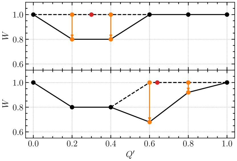
Figure 1: Schematic depiction of how $W$ is built with $N_{\mathrm{int}}=5$ and $s=0.4$. The red dot indicates the measured $Q^{\prime}$, while the orange points and arrows show the change in the $W$ function. The solid black line shows the updated $W$ function, the dashed line is the updated part of $W$ before the update. Top: $Q^{\prime}=0.3$. Bottom: $Q^{\prime}=0.64$.

Having defined our reweighting function in the domain of interest, we can start making reweighting updates. After letting the system thermalize with ordinary HMC updates, we begin building the reweighting function with reweighting updates. We start with a constant function $W(Q^{\prime})\equiv 1$. Our philosophy is that, whatever value of $Q^{\prime}$ we currently have, this value is presumably oversampled, and should be made less common by reducing $W(Q^{\prime})$ at the current value. Because $W$ is piecewise linear, the most local change we can make is to change the values at the two edges of the current interval. If $Q^{\prime}\in\omega_{i}$ with $i\neq 0$, only the corresponding values $W_{i}$ and $W_{i+1}$ are changed according to

$$W_{i} \to W_{i}-s(1-x),$$ (18)

$$W_{i+1} \to W_{i+1}-sx,$$ (19)

while the rest of the function remains unaffected. This procedure is illustrated in Fig. 1.

The first interval, $Q^{\prime}\in\omega_{0}$, is a special case. We need to remember that $Q^{\prime}$ is strictly positive and therefore $W_{0}$ will get updated less than the rest of the points. We correct for this via

$$W_{0} \to W_{0}-2s(1-x),$$ (20)

$$W_{1} \to W_{1}-sx.$$ (21)

The value of $s$ controls by how much $W$ changes each update. As soon as the gross features of $W$ arise, we decrease its value to slowly reach convergence. In order to do so it is instructive to introduce the notion of complete sweep. We refer to a complete sweep when the reweighting variable $Q^{\prime}$ ranges from $\omega_{0}$ to $\omega_{N_{\mathrm{int}}-1}$ and back to $\omega_{0}$. We count the number of updates needed to accomplish this and name it $M$. There is no need that it visits all intervals. The combination $\delta W=sM/N_{\mathrm{int}}$ tells us how much in average one point of $W$ has been changed during the completion of the last sweep. After each complete sweep we compute $\delta W$ and reduce $s$ to $s\to\text{max}\mathopen{}\mathclose{{}\left\{s/2,s\mathopen{}\mathclose{{}\left(1-\frac{\delta W}{1.5\times 2}}\right)}\right\}$. Therefore a sweep which changes a point in $W$ by of average more than 1.5 will lead to $s$ being cut in half, while a sweep which changes a point in $W$ by a smaller average amount will result in reducing $s$ less. After the value of $s$ has been updated, one resets the counter of $M$ back to zero waiting for the next completed sweep to appear and repeats the process.

Eventually, after several sweeps, once the gross features of $W$ have arisen, $\delta W$ will get small since $s$ is being consistently lowered, and the value of $M$ also should get smaller since fewer trajectories are needed for a completed sweep to appear (that is the whole idea of this update). We consider the procedure to be complete and $W(Q^{\prime})$ to be ready for use in a Monte Carlo study when $\delta W<0.1$. An animated GIF of how $W(Q^{\prime})$ evolves in this process is included in the Supplemental Material.

Our approach bears some similarities to the “metadynamics” approach Barducci et al. (2008); Laio et al. (2016); Sanfilippo et al. (2017) which has also been considered for this problem. One difference is in the way the $W(\xi)$ function is found. Some metadynamics implementations vary $W(\xi)$ throughout the course of the evolution, while others guess an initial value and keep it fixed. We advocate a hybrid approach where $W(\xi)$ is varied at first to optimize its form, and then frozen to produce a truly detailed-balance respecting evolution. We also propose a specific, we believe quite efficient, choice for the $W(\xi)$ function and its update. The other difference is that, in metadynamics, the $W(\xi)$ function is included as part of a “force” term in an HMC evolution, whereas we implement it purely through a Metropolis accept-reject step. The force-term approach is more efficient since HMC trajectories can be longer and because the acceptance rate is higher. But it requires evaluating the field-derivative of $\xi$, which may not always be possible or practical. For instance, because we implement gradient flow through stout smearing Morningstar and Peardon (2004), our $Q^{\prime}$ is a differentiable function of the link variables. But because we use many stout smearing steps, the differential expression is extremely unwieldy; within a quenched simulation our Metropolis implementation is much more efficient. But because the fermionic force term is also very expensive, the price may be worth paying in the unquenched case; indeed, after our first draft of this paper appeared but before its final publication, Bonati et al. succeeded in applying such a metadynamic method to the unquenched case Bonati et al. (2018).

Other approaches may also be available. Recently Bonati et al. Bonati and D’Elia (2018) presented several algorithms to solve the problem of topological freezing in the context of a simple quantum mechanical system which shares basic similarities with the problem at hand. In particular, Sec. IVF contains very similar concepts as the ones used in this paper. However it is not clear how the most effective algorithms they found could be generalized to the topology problem in QCD.

II.5 Parameters to Tune

The procedure described in the last section allows for the automated determination of $W(Q^{\prime})$, allowing for an efficient reweighting. But several parameters are still to be determined, and we found in practice that a certain amount of hand tuning was needed to select them.

First, there is the depth of gradient flow to use in establishing $Q^{\prime}$. (In practice we actually used stout smearing Morningstar and Peardon (2004) with step-size 0.06 as our gradient flow algorithm. This would be totally inadequate if our goal were a precision study of flowed operator expectation values, but here it is only important to suppress UV fluctuations, so a more efficient if less careful implementation of flow should be adequate.) We found that $t^{\prime}=0.24a^{2}$ is insufficient to separate configurations of different topology, while $t^{\prime}=0.42a^{2}$ is enough; larger amounts of gradient flow start to destroy the dislocations, which makes it more difficult to find the configurations intermediate between topological sectors. Optimally, one should perform several beginning-to-end determinations of $\chi$, each on the same lattice and temperature, but each time using different $t^{\prime}$ values, to do a systematic study of which choice leads to the highest statistics for a fixed computational effort; but we have not done this.

Second, there is the choice of the number and location of intervals. We found 20 intervals to be adequate except that there were two “corners” in the $W(Q^{\prime})$ function where its slope rather abruptly changes, see Fig. 3. These appear to be the points where the dominant type of configuration changes (regular thermal configuration to dislocation, dislocation to full-sized caloron), and the Monte Carlo simulation tends to get stuck at these points. We partly cured this by using more, narrower intervals at these points, which handles finer structure in the reweighting function and also leads to the algorithm spending more time near these points. So far we have done this by hand tuning, though presumably an automated method of interval adjustment could be developed, based for instance on the curvature of the determined $W[Q^{\prime}]$ function.

Next, there are the details of the parameter $s$ which controls how fast we adjust the $W(Q^{\prime})$ function. We tried variations on the procedure described above and found little change to the efficiency with which a good $W(Q^{\prime})$ is generated. In any case, if high statistics are desired, the Monte Carlo with fixed $W(Q^{\prime})$ takes most of the computational effort.

Next, there is the length of molecular-dynamics time used in the HMC algorithm updates. A larger HMC step leads to a larger change in the configuration, which is good because it more efficiently explores the phase space. But it leads to larger changes in $Q^{\prime}$ value and therefore to a higher rejection rate. So the HMC trajectory length needs to be tuned to provide about 50% acceptance rate in the $\mathrm{e}^{\Delta W}$ acceptance step. Again, 50% is a rule of thumb; a more careful analysis would compare the total achieved statistics at fixed numerical effort as a function of HMC trajectory length. To date we have not carried out such a study, and have instead used the 50% rule of thumb. Our results in what follow used HMC trajectory lengths of 0.2–0.25 $a$. We are well aware that such a small trajectory length will result in big autocorrelation effects between configurations. We have taken special care in providing a reliable error estimate by making a careful error analysis based on binning and jackknife Wolff (2004).

Finally, there is the choice of the final observable used to determine $\chi(T)$. Every 100 HMC trajectories, we make a measurement of $Q$ which we use in our statistical analysis of the susceptibility. We use $|Q|$ after some amount $t$ of gradient flow and set its value to 1 if $|Q|\geq Q_{\mathrm{thresh}}$ and to 0 if $|Q|<Q_{\mathrm{thresh}}$. (Configurations with $|Q|>1$ are very rare at the temperatures and for the volumes of interest, as we will establish in the next section.) This leaves open the exact choice of $t$, of $Q_{\mathrm{thresh}}$, and of gradient flow procedure (Wilson versus Zeuthen Ramos and Sint (2016)). All choices should lead to the same continuum limit and it is not expensive to sample using various choices and compare. This is what we will do; any difference between $\chi(T)$ values due to different threshold or flow depth will indicate deficiencies in our lattice spacing, and must be seen to vanish when we take the continuum limit.

III Results

Table 1: The lattices used in this work. Those labeled with A correspond to $2.5~{}T_{\mathrm{c}}$ while the Bs are simulations at $4.1~{}T_{\mathrm{c}}$.

Lat	$T/T_{\mathrm{c}}$	$6/g^{2}_{0}$	$\beta/a$	$L/a$	#Measurements	#Complete sweeps
$\text{A}_{1}$	2.5	6.507 Caselle et al. (2018)	6	16	61,759	591
$\text{A}_{2}$	2.5	6.722 Caselle et al. (2018)	8	16	96,068	263
$\text{A}_{3}$	2.5	6.903 Caselle et al. (2018)	10	24	66,840	195
$\text{B}_{1}$	4.1	6.883 Giusti and Meyer (2011)	6	16	70,699	313
$\text{B}_{2\mathrm{a}}$	4.1	7.135 Giusti and Meyer (2011)	8	8	50,992	94
$\text{B}_{2\mathrm{b}}$	4.1	7.135 Giusti and Meyer (2011)	8	12	50,390	82
$\text{B}_{2\mathrm{c}}$	4.1	7.135 Giusti and Meyer (2011)	8	16	52,900	145
$\text{B}_{2\mathrm{d}}$	4.1	7.135 Giusti and Meyer (2011)	8	24	74,900	168
$\text{B}_{2\mathrm{e}}$	4.1	7.135 Giusti and Meyer (2011)	8	32	72,800	151
$\text{B}_{3}$	4.1	7.325 Giusti and Meyer (2011)	10	24	82,663	104

Our goal in this paper is to demonstrate our method and show that it can obtain statistically powerful results at high temperatures in a range of lattice spacings and volumes. With this in mind, we study 10 different lattices, as listed in Tab. 1. We use the Wilson gauge action at two temperatures corresponding to $2.5~{}T_{\mathrm{c}}$ and $4.1~{}T_{\mathrm{c}}$; the values of $\beta$ are taken from Refs.  Caselle et al. (2018); Giusti and Meyer (2011). At the higher temperature we consider aspect ratios between 1:1 and 4:1 with $N_{\tau}=8$ and at both temperatures we consider lattice spacings with $N_{\tau}=6,8,10$ with an aspect ratio of about 2.5:1. This allows one study of the volume scaling, and lets us take the continuum limit, but it is not sufficient to consider both limits simultaneously. All calculations were carried out over a six month period on one eight-core desktop machine and one server node with two Xeon-Phi (KNL) CPUs. By modern standards this is an extremely modest computational budget.

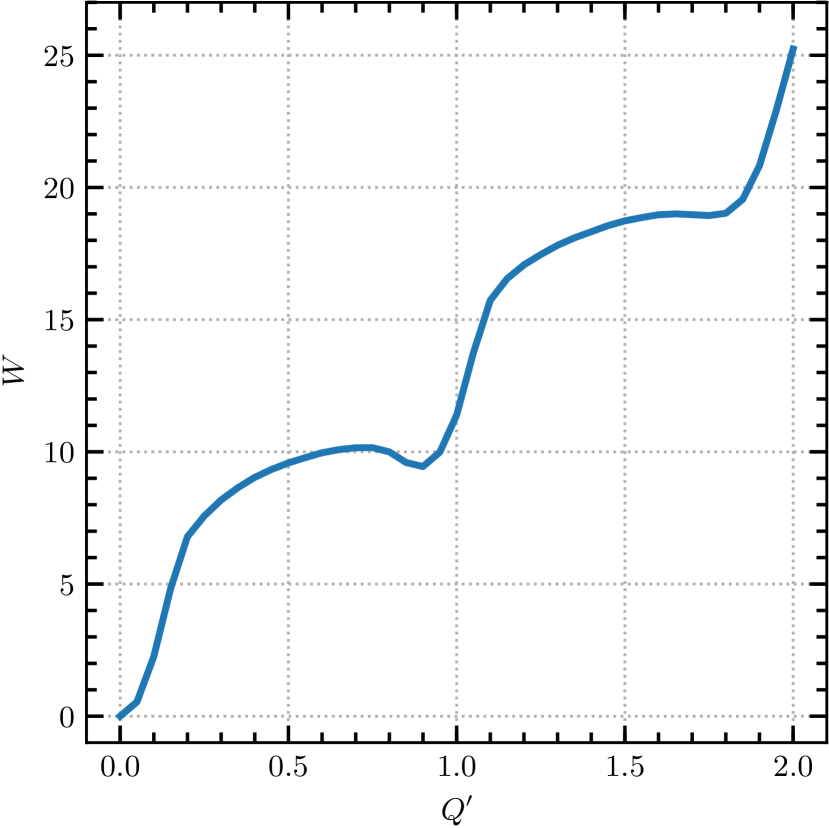
Figure 2: $W$ function of $6\times 16^{3}$ lattice at $2.5~{}T_{\mathrm{c}}$ (Lattice A₁).

The first question is: is it sufficient so sample only $Q=0$ and $|Q|=1$ sectors, or are larger values of $|Q|$ also important in establishing the topological susceptibility? To study this, first look at Eq. (6) and consider what happens when we use $Q$ with a threshold as the observable:

$$\begin{split}\langle Q^{2}\rangle&=\frac{\sum_{i}^{N}Q_{i}^{2}\mathrm{e}^{-W(Q^{\prime}_{i})}}{\sum_{i}^{N}\mathrm{e}^{-W(Q^{\prime}_{i})}}\\ &\simeq\frac{\sum_{i:|Q|=1}\mathrm{e}^{-W(Q^{\prime}_{i})}+\sum_{i:|Q|=2}4\mathrm{e}^{-W(Q^{\prime}_{i})}+\ldots}{\sum_{i:|Q|=0}\mathrm{e}^{-W(Q^{\prime}_{i})}},\end{split}$$ (22)

where in the numerator we only have to sum over $|Q|=1$ and higher configurations since $Q=0$ does not contribute, while in the denominator we only sum over $|Q|=0$ because they completely dominate the ensemble. Clearly we need both $Q=0$ and $|Q|=1$ configurations to perform the calculation; but if our accuracy goal is $10\%$, then we only need $|Q|=2$ and higher if the total probability to be in one of these states is at least 2.5% of that for $|Q|=1$ states. Therefore we carried out the construction of $W(Q^{\prime})$ in the domain $0\leq Q^{\prime}\leq 2$, shown in Fig. 2, for the lower temperature we study and a $6\times 16^{3}$ lattice (Lattice A₁). We see immediately from the figure that $Q^{\prime}>1.5$ configurations require a reweighting of $\mathrm{e}^{-18}$ to occur, while $Q^{\prime}>0.75$ configurations occur already with an $\mathrm{e}^{-9}$ reweighting. For our $t^{\prime}$ values the $|Q|=1$ values all have $Q^{\prime}>0.7$ and $|Q|=2$ values all have $Q^{\prime}>1.5$, so this means that $|Q|=2$ configurations are suppressed relative to $|Q|=1$ configurations by about $\mathrm{e}^{-9}$. Therefore $|Q|=2$ plays a tiny role in Eq. (22) and can be safely ignored. In a larger volume, an instanton gas estimate says that the $|Q|=1$ configurations should get more common with $V$ and the $|Q|=2$ configurations should get more common with $V^{2}$. So $|Q|=2$ would start to become relevant in a box with an aspect ratio of about 15. Such enormous lattices are not needed to study $\chi(T=2.5~{}T_{\mathrm{c}})$, and so we do not need to consider $|Q|\geq 2$. This conclusion only strengthens for a larger $T$ where the susceptibility is still smaller. Obviously, at some lower temperature it will break down and we will need many topological sectors; so every time we go to lower temperatures we must revisit this issue.

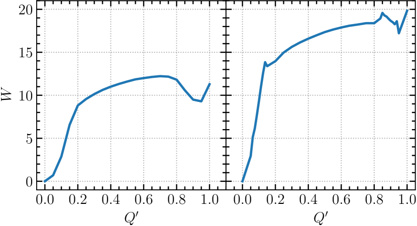
Figure 3: $W$ functions of $8\times 16^{3}$ lattice. Left: $2.5~{}T_{\mathrm{c}}$ (Lattice A₂). Right: $4.1~{}T_{\mathrm{c}}$ (Lattice B_2c).

We proceed to compute the reweighting function $W(Q^{\prime})$ using $Q_{\mathrm{max}}^{\prime}=1$. Two examples are shown in Fig. 3. In each case there is a deep minimum at $Q^{\prime}=0$ corresponding to ordinary $Q=0$ configurations and a much shallower minimum near $Q^{\prime}=1$, corresponding to $\mathopen{}\mathclose{{}\left|Q}\right|=1$ configurations. The broad plateau in between can be understood as configurations containing a dislocation. The sharp features in the $4.1~{}T_{\mathrm{c}}$ plot are caused by our abruptly adjusting the width of our intervals. At finer lattices (larger $N_{\tau}$) the $\mathopen{}\mathclose{{}\left|Q}\right|=1$ minimum becomes deeper (or more accurately, the barrier gets higher), as the size of physical calorons becomes more different from the lattice spacing.

Table 2: This table shows $-\ln\mathopen{}\mathclose{{}\left(\chi/T_{\mathrm{c}}^{4}}\right)$ for all points plotted in Figs. 4–6. Errors are statistical only.

Flow:	Wilson	Wilson	Zeuthen	Zeuthen	Zeuthen	Zeuthen
$t/a^{2}$:	$1.2$	$2.4$	$1.2$	$2.4$	$2.4$	$2.4$
$Q_{\mathrm{thresh}}$:	0.7	0.7	0.7	0.5	0.7	0.9
Lat.	$-\ln\mathopen{}\mathclose{{}\left(\chi/T_{\mathrm{c}}^{4}}\right)$	$-\ln\mathopen{}\mathclose{{}\left(\chi/T_{\mathrm{c}}^{4}}\right)$	$-\ln\mathopen{}\mathclose{{}\left(\chi/T_{\mathrm{c}}^{4}}\right)$	$-\ln\mathopen{}\mathclose{{}\left(\chi/T_{\mathrm{c}}^{4}}\right)$	$-\ln\mathopen{}\mathclose{{}\left(\chi/T_{\mathrm{c}}^{4}}\right)$	$-\ln\mathopen{}\mathclose{{}\left(\chi/T_{\mathrm{c}}^{4}}\right)$
$\text{A}_{1}$	7.37(07)	7.52(07)	7.24(07)	7.31(07)	7.35(07)	7.53(07)
$\text{A}_{2}$	7.79(10)	7.85(10)	7.74(10)	7.76(10)	7.78(10)	7.85(10)
$\text{A}_{3}$	8.09(16)	8.11(16)	8.07(16)	8.08(16)	8.08(16)	8.11(16)
$\text{B}_{1}$	10.21(07)	10.41(07)	10.04(07)	10.14(07)	10.19(07)	10.43(07)
$\text{B}_{2\mathrm{a}}$	12.74(09)	13.11(10)	12.47(10)	12.65(09)	12.75(10)	13.17(10)
$\text{B}_{2\mathrm{b}}$	11.90(10)	12.08(11)	11.74(10)	11.84(10)	11.89(11)	12.10(11)
$\text{B}_{2\mathrm{c}}$	11.36(11)	11.46(12)	11.26(11)	11.31(11)	11.34(11)	11.46(12)
$\text{B}_{2\mathrm{d}}$	11.10(13)	11.18(13)	11.03(13)	11.07(13)	11.09(13)	11.18(13)
$\text{B}_{2\mathrm{e}}$	11.16(14)	11.24(14)	11.07(13)	11.12(14)	11.15(14)	11.24(14)
$\text{B}_{3}$	11.76(17)	11.80(17)	11.72(17)	11.74(17)	11.76(17)	11.80(17)

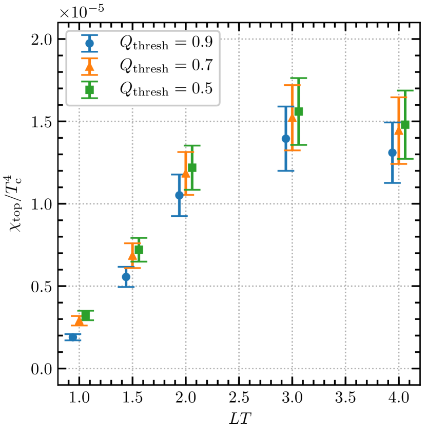
Figure 4: Finite volume dependence of the susceptibility at $N_{\tau}=8$ and $T=4.1~{}T_{\mathrm{c}}$ (Lattices B_2a through B_2e), using Zeuthen flow with $t=2.4a^{2}$ and three different values of $Q_{\mathrm{thresh}}$ (points have been displaced for reasons of visibility).

With the $W(Q^{\prime})$ reweighting functions in hand, we proceed to evaluate the topological susceptibility via Eq. (22). For completeness, we present all of our results in Tab. 2. The errors in the table always represent our statistical uncertainty, for the given lattice spacing, temperature, volume, and $Q$ definition. Systematic errors, particularly those associated with the continuum and large-volume limits, must be determined by comparing results from different lattices. First, consider the large-volume limit, by analyzing $\chi$ as a function of aspect ratio, shown in Fig. 4. The figure evaluates $Q$ after $t=2.4a^{2}$ of improved (Zeuthen) gradient flow, and considers three different values for the threshold to distinguish between $|Q|=1$ and $Q=0$: $Q_{\mathrm{thresh}}=0.5$, 0.7, and 0.9. The figure shows that, as expected, aspect ratios smaller than 2 are badly discrepant; but the difference between an aspect ratio of 2 and 4 is of an order of tens of a percent, and is not statistically significant. It appears that large-volume behavior sets in at a modest aspect ratio between 2 and 3 (at this temperature). Therefore in this exploratory study, we will only consider the continuum limit for an aspect ratio of about 2.5. The figure also shows that although the value of $Q_{\mathrm{thresh}}$ introduces a systematic effect (the lower the threshold, the higher the determined $\chi$ value), this effect is statistically irrelevant already at $LT<1.5$ and becomes even smaller for larger volumes (and finer lattices, see Tab. 2); in what follows we will use $Q_{\mathrm{thresh}}=0.7$.

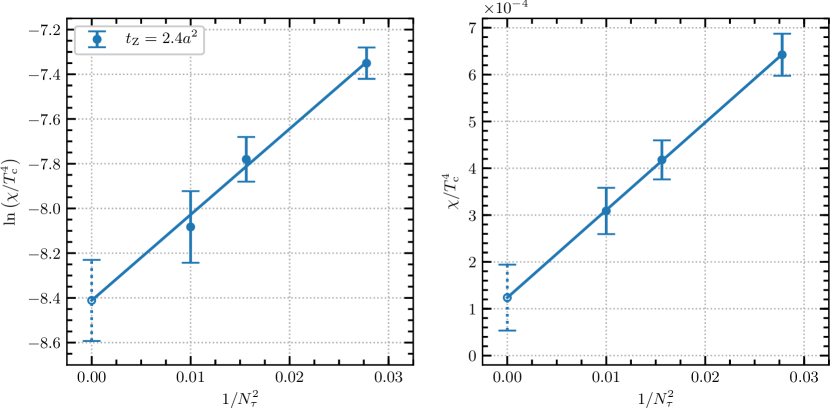
Figure 5: Continuum extrapolation at $T=2.5~{}T_{\mathrm{c}}$ based on lattices A₁, A₂, A₃, carried out in terms of $\chi(T)$ directly (right) and $\ln\mathopen{}\mathclose{{}\left(\chi(T)}\right)$ (left) using Zeuthen flow with $t=2.4a^{2}$ and $Q_{\mathrm{thresh}}=0.7$.

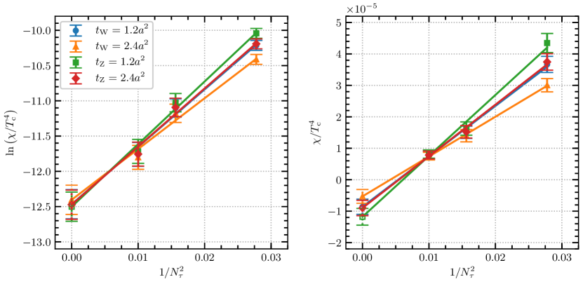
Figure 6: Same as Fig. 5 except for $T=4.1~{}T_{\mathrm{c}}$, using lattices B₁, B_2d, B₃. In addition we have shown separately the measured values for two amounts of flow $t=1.2a^{2}$ and $t=2.4a^{2}$ and for two flow actions (Wilson and Zeuthen). Note that the linear-extrapolated continuum limit is negative for all choices.

Finally we consider the continuum extrapolation, using three lattice spacings with $N_{\tau}=6,$ 8, and 10. We show this for $T=2.5~{}T_{\mathrm{c}}$ in Fig. 5 and $T=4.1~{}T_{\mathrm{c}}$ in Fig. 6 (note that the $N_{\tau}=8$ lattice has a slightly different aspect ratio than the $N_{\tau}=6,10$ lattices; smaller for $2.5~{}T_{\mathrm{c}}$ and larger for $4.1~{}T_{\mathrm{c}}$). At the higher temperature, we show results for two flow depths ($t=1.2a^{2}$ and $t=2.4a^{2}$) and two choices of flow action (Wilson and Zeuthen). The different $Q$ definitions differ significantly for $N_{\tau}=6$ (note that the determinations use the same Markov chain, so the errors are highly correlated and the difference is statistically very significant) but are nearly indistinguishable for $N_{\tau}=10$; so issues of topology definition are seen to become small on fine lattices. The choice of topology definition is irrelevant in the continuum limit if we extrapolate in terms of $\ln\mathopen{}\mathclose{{}\left(\chi}\right)$.

However, if we attempt to extrapolate $\chi\mathopen{}\mathclose{{}\left(T,a^{2}}\right)$ linearly against $a^{2}$, we get very poor behavior. At $T=2.5~{}T_{\mathrm{c}}$ the two continuum limits, based on extrapolating $\ln\mathopen{}\mathclose{{}\left(\chi}\right)$ and extrapolating $\chi$ directly, differ by more than their error bars. And at $T=4.1~{}T_{\mathrm{c}}$, the linear extrapolations of $\chi(T)$ using different definitions of topology are incompatible, and each definition leads to a negative extrapolated value, which is clearly unphysical. On the other hand, if we perform a linear extrapolation of $\ln\mathopen{}\mathclose{{}\left(\chi}\right)$ against $a^{2}$, the different definitions of topology produce compatible results, which are finite and physical. The reason that one should extrapolate in $\ln\mathopen{}\mathclose{{}\left(\chi}\right)$ and not in $\chi$ directly, as we understand it Jahn et al. (2018), is that the topological susceptibility is controlled by the exponential suppression of the caloron action $\exp\mathopen{}\mathclose{{}\left(-S_{\mathrm{caloron}}}\right)=\exp\mathopen{}\mathclose{{}\left(-8\pi^{2}/g^{2}(\mu\sim T)}\right)$. This action receives multiplicative $\mathcal{O}\mathopen{}\mathclose{{}\left(a^{2}}\right)$ lattice corrections: $\chi\propto\exp(-S)\to\exp\mathopen{}\mathclose{{}\left(-[1-\mathcal{O}(a^{2}T^{2})]\,S}\right)$. That is, the $a^{2}$ corrections are best viewed as a shift in the caloron action and therefore in the logarithm of the susceptibility. Therefore an extrapolation of $\ln\mathopen{}\mathclose{{}\left(\chi(T)}\right)$ in terms of $a^{2}$ is better justified, and better behaved. Indeed, Fig. 3 shows that $S_{\mathrm{caloron}}$ is about twice as large at $T=4.1~{}T_{\mathrm{c}}$ than at $T=2.5~{}T_{\mathrm{c}}$; so the slope of the extrapolation should be twice as large in the left panel of Fig. 6 as in Fig. 5, which it is. Therefore this picture of the nature of $a^{2}$ errors is consistent with our findings, and an extrapolation of $\ln\mathopen{}\mathclose{{}\left(\chi}\right)$ against $a^{2}$ is the theoretically best motivated way to extrapolate to the continuum.

IV Discussion

We have presented a methodology for applying reweighting Berg and Neuhaus (1991) to the measurement of topology in high temperature pure-glue SU(3) QCD. Our approach involves reweighting in terms of a “poor man’s” topological measurement $Q^{\prime}$ ($Q$ measured after a small amount of flow $t^{\prime}=0.42a^{2}$ and using an $a^{2}$ improved topological density operator). There is then a two-stage simulation; first we simulate while dynamically changing our reweight function, to determine the form of the reweight function. Then we fix the reweight function and perform a Monte Carlo simulation to determine the topological susceptibility.

The method is effective; with modest numerical resources we are able to treat $T=4.1~{}T_{\mathrm{c}}$ up to an aspect ratio of 4 and up to a lattice spacing with $N_{\tau}=10$, obtaining good statistics. Making a full continuum extrapolation but at a modest aspect ratio of 2.5 (extrapolating the $t=2.4a^{2}$, Zeuthen flow results), we find

$$\begin{split}\frac{\chi(T=2.5~{}T_{\mathrm{c}})}{T_{\mathrm{c}}^{4}}=2.22\times 10^{-4}\ \mathrm{e}^{\pm 0.18},\\ \frac{\chi(T=4.1~{}T_{\mathrm{c}})}{T_{\mathrm{c}}^{4}}=3.83\times 10^{-6}\ \mathrm{e}^{\pm 0.21}.\end{split}$$ (23)

Our results at individual $N_{\tau}$ values are consistent with previous studies; our $\mathrm{A}_{1}$ lattice gives the same susceptibility as found by Berkowitz et al Berkowitz et al. (2015), and our results at $4.1\,T_{\mathrm{c}}$ and $N_{\tau}=6,8$ (lattices $\mathrm{B}_{1}$ and $\mathrm{B}_{2\mathrm{e}}$) appear compatible with those at $4.0\,T_{\mathrm{c}}$ from Borsanyi et al Borsanyi et al. (2016a), who have significantly larger statistical errors despite applying much more numerical effort. Those authors also provide a continuum-extrapolated functional fit for $\chi(T)$, which is in reasonable agreement with our results; applying their fit form to the temperatures we studied, we obtain $\chi(2.5~{}T_{\mathrm{c}})=1.9\times 10^{-4}~{}T_{\mathrm{c}}^{4}$ and $\chi(4.1~{}T_{\mathrm{c}})=5.6\times 10^{-6}~{}T_{\mathrm{c}}^{4}$.

Our results teach a few other lessons. On a lattice with $N_{\tau}=6$, $\chi$ is sensitive to the exact definition of topology (depth of flow, flow action, threshold). This dependence is nearly gone by $N_{\tau}=10$ and seems not to affect the continuum extrapolation. The continuum extrapolation should be performed in terms of $\ln\mathopen{}\mathclose{{}\left(\chi}\right)$, not in terms of $\chi$ itself. The continuum extrapolation corrections to $\ln\mathopen{}\mathclose{{}\left(\chi}\right)$ can be large and are larger at higher temperature. None of these lessons should be surprising Jahn et al. (2018).

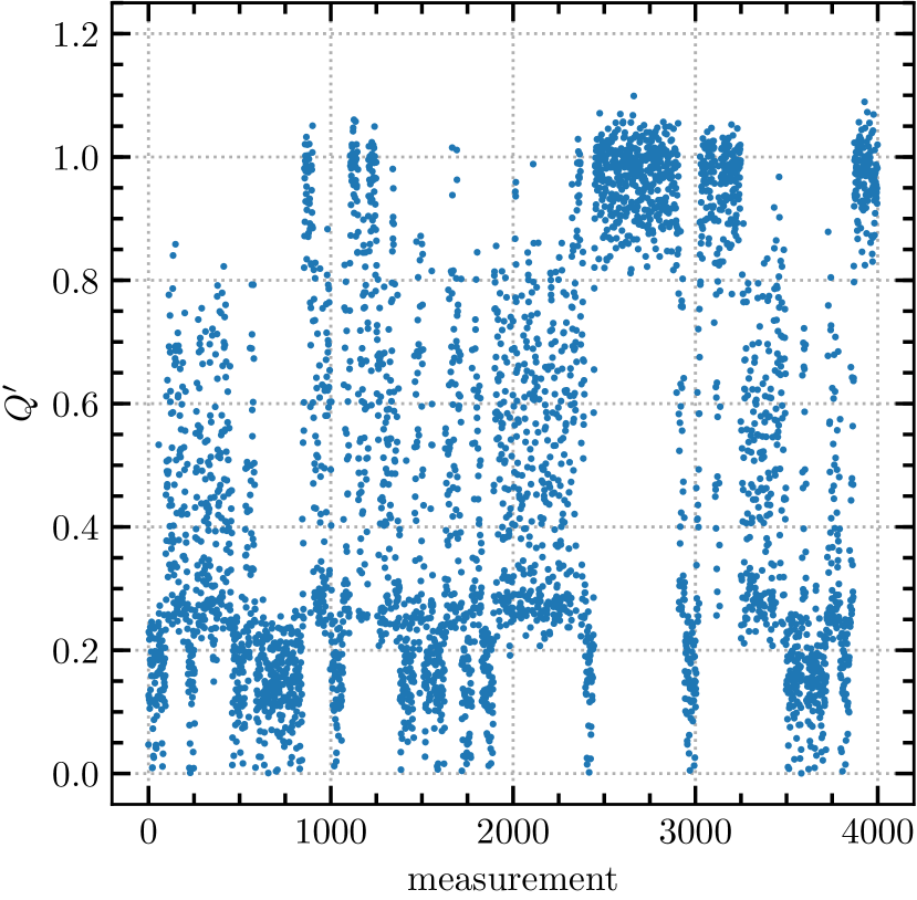
Figure 7: Piece of a Markov-chain history of $Q^{\prime}$ against measurement number, for lattice B_2d. The reweighting allows efficient sampling in three regions, $0<Q^{\prime}<0.27$, $0.20<Q^{\prime}<0.85$, and $0.8<Q^{\prime}<1.05$, but has difficulty moving between these regions.

We should not claim that our technique solves all problems, however. Looking at the $Q^{\prime}$ value as a function of measurement number for a short portion of a Markov chain evolution, shown in Fig. 7, we see that despite our reweighting function, there are a few points where the simulation gets “stuck.” It moves easily in the range $0<Q^{\prime}<0.27$ and similarly moves easily across $0.2<Q^{\prime}<0.85$; but it has difficulty moving from one of these ranges to the other. There is a similar “barrier” around $Q^{\prime}=0.8$. These problems become more severe as we move to larger $N_{\tau}$. We believe that this occurs because $Q^{\prime}$ is an incomplete descriptor which is missing some other information which distinguishes between these regions. We partly overcame this problem by making more, narrower reweighting bins in these overlap regions; our reweighting procedure causes the Markov chain to spend approximately equal time in each bin, so narrower bins cause more time to be spent in these regions, which helps the Markov chain to find the way between the different regions. (This is the reason for the cuspy discontinuities in Fig. 3.) However, while this helps, it hardly solves the problem, as Fig. 7 attests. We are searching for one or more additional observables to serve as further reweighting variables in the hopes of improving this sampling. Another inefficiency is that the number of updates needed to move between topological sectors does not improve as we increase the volume. Therefore, to achieve a given level of statistics, the numerical effort must grow linearly with the volume. We do not foresee any solution to this problem.

Conceptually there are no obstacles to applying our technique to the unquenched case (at high temperatures where only one or a few topological sectors are relevant). However, we expect doing so to be numerically more difficult. First, the HMC algorithm requires far more computer power with fermions. Second, the $Q=1$ sector has near-zero eigenvalues, while the $Q=0$ sector should have the smallest eigenvalue close to $\pi T$. The chiral limit should be severe. Third, the characteristic size of a caloron is smaller with light quarks than without Gross et al. (1981), and therefore the lattice spacing should need to be smaller ($N_{\tau}$ values larger) than what we need in pure glue. But we view these added numerical challenges as reasons that such studies should use reweighting. The temperature range where topology is relevant for axions is $3\,T_{\mathrm{c}}$ to $7\,T_{\mathrm{c}}$ Moore (2018), where topology is quite suppressed and only the $|Q|=1$ sector should contribute. To overcome the challenges just mentioned in this temperature range, we absolutely need the improvement in statistical sampling of $|Q|=1$ from reweighting if any statistical power is to be achieved.

It is less clear that our approach has applications at lower temperatures where multiple topological sectors are relevant. We might hope that a similar reweighting method might help with the topological-sector sampling problem, which afflicts fine lattices. However, it is not clear to us that $Q^{\prime}$ will be an effective reweighting variable in this case. We leave study of this problem for future work.