Confidence Interval Estimators for MOS Values

Abstract

For the quantification of QoE, subjects often provide individual rating scores on certain rating scales which are then aggregated into Mean Opinion Scores (MOS). From the observed sample data, the expected value is to be estimated. While the sample average only provides a point estimator, confidence intervals (CI) are an interval estimate which contains the desired expected value with a given confidence level. In subjective studies, the number of subjects performing the test is typically small, especially in lab environments. The used rating scales are bounded and often discrete like the 5-point ACR rating scale. Therefore, we review statistical approaches in the literature for their applicability in the QoE domain for MOS interval estimation (instead of having only a point estimator, which is the MOS). We provide a conservative estimator based on the SOS hypothesis and binomial distributions and compare its performance (CI width, outlier ratio of CI violating the rating scale bounds) and coverage probability with well known CI estimators. We show that the provided CI estimator works very well in practice for MOS interval estimators, while the commonly used studentized CIs suffer from a positive outlier ratio, i.e., CIs beyond the bounds of the rating scale. As an alternative, bootstrapping, i.e., random sampling of the subjective ratings with replacement, is an efficient CI estimator leading to typically smaller CIs, but lower coverage than the proposed estimator.

I Introduction

Quality of Experience (QoE) research commonly relies on the collection of subjective ratings from a chosen panel of users to quantify various QoE dimensions (also referred to as QoE features [1]), e.g., related to perceived audio/visual quality, perceived usability, or overall perceived quality. While various rating scales have been used in both the user experience (UX) and QoE research fields, the results of subjective studies reported by the QoE community have to a large extent relied on the use of a standardized 5-point Absolute Category Rating (ACR) scale to calculate Mean Opinion Score (MOS) values. While it has been argued that researchers should go beyond the MOS in their studies [2] in order to consider different applications and user diversity, MOS estimates remain a staple of the QoE literature.

In this context, the statistical analysis of subjective study results, subsequently used to derive QoE estimation models [3], relies on the estimation of confidence intervals (CIs) to quantify the significance of MOS values per test condition. Challenges arise in dealing with uncertainties resulting from problems such as ordering effects and subject biases [3, 4]. Such statistical uncertainties are expressed in terms of CIs. Given the nature of conducting QoE studies, two main issues arise. Firstly, rating scales used in quantitative QoE evaluation are bounded at both ends. Therefore, the individual rating scores $Y$ of a subject are limited. However, for the calculation of CIs, normal distributions (due to central limit theorem) or Student’s t-distribution are used, which are unbounded.

Secondly, due to the inherent complexity of running subjective studies, resulting in a compromise between a large number of test conditions and participant fatigue, the number $n$ of test subjects taking part in a study is generally small, in particular when running tests in a lab environment. We note that while methods such as crowdsourcing may be utilized to obtain a much larger population sample, in many cases the specifics of the study call for a controlled lab environment. As an example, and bearing in mind that the number of required participants clearly depends on the test design, number of test conditions, and target population, the ITU-T recommends a minimum of 24 subjects (controlled environment) or 35 subjects (public environment) for subjective assessment of audiovisual quality [5]. ITU-T Recom. P.1401 further states that if fewer than 30 samples are used, the normal distribution starts to become distorted and calculation of CIs based on normality assumptions are no longer valid. In cases with fewer than 30 samples, P.1401 advocates the use of the Student t-distribution when calculating CIs.

Given the aforementioned issues, we highlight that commonly used CI estimators do not work properly for small sample sizes, as the normal distribution assumption may not be valid, and that they violate the bounds of the rating scale. In this paper we review statistical approaches in the literature for their application in the QoE domain for MOS interval estimation (instead of having only a point estimator, which is the MOS). Due to space restrictions, we consider only discrete rating scales, and test the CI estimators in terms of efficiency (CI width), coverage (how many CIs overlap the true mean value), and outlier ratio.

The remainder of this paper is organized as follows. Section II provides the background on CIs such as the central limit theorem, used to derive CI estimators. Section III considers common estimators for the MOS and introduces some estimators based on binomal distributions that are suitable for MOS CI estimation. It also discusses other non-commonly used methods in the QoE community, such as simultaneous CI and bayesian approaches for multinomial distributions, as well as bootstrapping CI. Section IV defines various scenarios for evaluating the performance of the estimators in terms of coverage, outlier ratio, and CI width. Section V concludes this work and gives some recommendations on CI estimators for MOS values in practice.

II Background

For the sake of readability, we briefly state the definitions and theorems used to obtain an interval estimate, denoted confidence intervals in the following. Table I provides a summary of the notation used throughout the paper.

• Let $X$ be a random sample from a probability distribution with statistical parameter $\theta$, which is a quantity to be estimated. The confidence interval $[\theta_{0},\theta_{1})$, is obtained by

  $$P(\theta_{0}\leqslant\theta<\theta_{1})=1-\alpha,\ 0<\alpha<1$$ (1)

  where $(1-\alpha)$ is the confidence coefficient (or degree of confidence). The confidence interval contains the statistical parameter $\theta$ with probability $1-\alpha$.

• Let $X$ be a random sample of size $n$ ($X=\{X_{1},X_{2},\ldots,X_{n}\}$) taken from a population with expected value $\mathrm{E}(X_{i})=\mu$ and variance $\mathrm{Var}(X_{i})=\sigma^{2}<\infty$, $\ i=1,2,\ldots,n$, then the sample mean $\hat{X}$ asymptotically follows a normal distribution with expected value $\mu$ and variance $\sigma^{2}/n$ as $n\to\infty$.

  $$\hat{X}\mathop{\sim}_{n\to\infty}\mathcal{N}\left(\mu,\frac{\sigma^{2}}{n}\right)$$ (2)

• The confidence interval for the sample mean $\hat{X}$, with $E[X]=\theta$ and standard error of the sample mean $S/\sqrt{n}$ according to CLT, can be obtained by

  $$\hat{X}\pm z_{\alpha/2}\cdot\frac{S}{\sqrt{n}}$$ (3)

  where $z_{\alpha/2}$ is the $\alpha/2$-quantile of the standard normal distribution $N(0,1)$. $S^{2}$ estimates the unknown variance $\sigma^{2}$.

This assumes that the sample size $n$ is large, and that the sampling distribution is symmetric, which is not always the case. In the following, we detail how to establish a confidence interval in the case of a sampling distribution whose density function is symmetric or non-symmetric around the mean.

Note that the variance of a sample mean, ${\rm{Var}}\!\left[\hat{X}\right]={\rm{Var}}\!\left[\frac{1}{n}\sum_{i=1}^{n}X_{i}\right]={\rm{Var}}\!\left[X\right]/n$, where ${\rm{Var}}\!\left[X\right]$ is the variance of the sample $X$. This implies that when $n\to\infty$ then ${\rm{Var}}\!\left[\hat{X}\right]\to 0$ while ${\rm{Var}}\!\left[X\right]\to\sigma^{2}$.

TABLE I: Notation and variables used in the paper.

Variable	Description
$Y_{x}$	random variable of user ratings for test condition $x$
$k$	users rate on a discrete $k$-point rating scale from $1,\dots,k$
$n$	number of users rating the test condition
$m$	number of test conditions (TC)
$r$	number of simulation runs
$y_{u,x,i}$	sampled user rating for user $u$, TC $x$ and simulation run $i$
$\hat{Y}_{x,i}$	MOS, i.e. sample mean over user ratings, for TC $x$ and run $i$
$\gamma$	confidence level
$\alpha$	significane level, e.g. $\alpha=0.05$; it is $\alpha=1-\gamma$

III Confidence Interval Estimators for MOS

III-A Problem Formulation

We assume we have a discrete rating scale with $k$ rating items, leading to a multinominal distribution, which is a generalization of the binomial distribution. For a certain test condition, $n$ users rate the quality on a discrete $k$-point rating scale, e.g., $k=5$ for the commonly used 5-point ACR scale. Each scale item is selected with probability $p_{i}$ for $i=1,\dots,k$; $\sum_{i=1}^{k}p_{i}=1$.

The $n$ users rate quality as one of the $k$ categories. Samples $(n_{1},\dots,n_{k})$ indicate the number of ratings obtained per category, with $\sum_{i=1}^{k}n_{i}=n$ (i.e., each user has provided one rating). With each category having a fixed probability $p_{i}$, the multinomial distribution gives the probability of any particular combination of numbers $n_{i}$ of successes for the various categories (under the condition $n_{k}=n-\sum_{i=1}^{k-1}n_{i}$)

$$P(N_{1}=n_{1},\dots,N_{k}=n_{k})=\frac{n!}{n_{1}!\cdots n_{k}!}p_{1}^{n_{1}}\cdots p_{k}^{n_{k}}$$ (4)

In QoE tests, we are interested in the rating of an arbitrary user. The marginal distribution (when $n=1$) with $p_{i}$ estimates the the expected rating ${\rm{E}}\!\left[Y\right]$ by the sample mean $\hat{Y}$ (aka MOS), assuming a linear rating scale.

$$\hat{Y}=\frac{1}{k}\sum_{i=1}^{k}ip_{i}$$ (5)

We denote $Y$ as a random variable of the rating of the users. We observe a sample $Y_{1},\dots,Y_{n}$ with $Y_{i}\in\{1,\dots,k\}$. As previously stated, in subjective QoE tests, the number $n$ of users is typically not very high. From the samples $(n_{1},\dots,n_{k})$, the MOS and CI can be estimated. However, given the use of a bounded rating scale and small sample size, existing estimators of CI do not follow the CLT and might be asymmetric around the sample mean, and will potentially violate the bounds of the rating scale, i.e., $\theta_{0}<1$ and/or $\theta_{1}>k$.

III-B Regular Normal and Student’s t-distribution

The most common way of constructing a CI from a set of samples, $X=\{X_{1},\cdots,X_{n}\}$, is to apply the CLT. When the variance of $X$ is not known, then the quantile $t_{\alpha/2,n-1}$ must be taken from a Student’s t-distribution with confidence level $1-\alpha$ and $n-1$ degrees of freedom, unless the number of samples are sufficiently large ($n>30$ according to ITU-T recommendation P.1401). Then the quantiles in the Student’s t-distribution and standard Normal distributions are approximately the same.

The CI for both Student’s t-distribution and Normal distribution is estimated by use of (3), the only difference is the quantiles.

Observe; truncating the upper and lower bounds, i.e., $\theta^{*}_{0}=\max(1,\theta_{0})$ and/or $\theta^{*}_{1}=\min(k,\theta_{1})$ is not correct.

III-C Simultaneous CIs for Multinomial Distribution

A complementary approach is to consider the multinomial proportions $p_{i}$ of user ratings on the scale for item $i$ and then to derive exact confidence coefficients of simultaneous CI for those multinomial proportions. A method for computing the CIs for functions of the multinomial proportions is proposed in [6] which can be directly applied to the computation of the MOS, see  Eq.(5). There are $n_{i}$ user ratings for category $i$ and $\chi_{1-\alpha/k}$ is the quantile of the $\chi^{2}$-distribution with one degree of freedom considering $k$ simultaneous CIs. The MOS is $\hat{Y}=\sum_{i=1}^{k}i\frac{n_{i}}{n}$.

$$\sum_{i=1}^{k}i\frac{n_{i}}{n}\pm\sqrt{\frac{\chi_{1-\alpha/k}}{n}\left(\sum_{i=1}^{k}i^{2}\frac{n_{i}}{n}\right)-\left(\sum_{i=1}^{k}i\frac{n_{i}}{n}\right)^{2}}$$ (6)

III-D Using Binomial Proportions for Discrete Rating Scales

The shifted binomial distribution can be used as an upper bound distribution for user rating distributions when users rate on a $k$-point rating scale ($1,\dots,k$). The binomial distribution leads to high standard deviations in QoE tests [7] and follows exactly the SOS hypothesis with parameter $a=1/{k_{0}}$ with ${k_{0}}=k-1$.

Let us consider $n$ users. Assume the user ratings follow a shifted binomial distribution, $Y_{i}\sim\mathrm{Bino}({k_{0}},p)+1$. Then, the sum of the user ratings follows also a binomial distribution.

$$Y=\sum_{i=1}^{n}Y_{i}\sim\mathrm{Bino}(\sum_{i=1}^{n}{k_{0}},p)+1=\mathrm{Bino}(n\cdot{k_{0}},p)+1$$ (7)

and then $\hat{Y}=\frac{1}{n}\sum_{i=1}^{n}Y_{i}\sim\mathrm{Bino}(\frac{1}{n}\sum_{i=1}^{n}{k_{0}},p)+1=\mathrm{Bino}(\cdot{k_{0}},p)+1$. Due to differences among users, it may be $p_{i}\neq p_{j}$ for users $i$ and $j$. The binomial sum variance inequality can be used to derive an upper bound. Let us consider $Y=\sum_{i=1}^{n}Y_{i}$, which does not follow a binomial distribution. We define $Z\sim\mathrm{Bino}(n\cdot{k_{0}},\bar{p})+1$ with $\bar{p}=\frac{1}{n}\sum_{i=1}^{n}p_{i}$. As a result of the binomial sum variance inequality we observe that the variance of $Z$ is an upper bound for QoE tests.

$${\rm{Var}}\!\left[Y\right]<{\rm{Var}}\!\left[Z\right]$$ (8)

Hence, we may use $\hat{Z}$ instead of $\hat{Y}$ to derive conservative CIs for the MOS based on the CI $[\hat{p}_{0};\hat{p}_{1}]$ for the unknown $p$.

$$[\hat{Z}_{0},\hat{Z}_{1}]=[\hat{p}_{0},\hat{p}_{1}]\cdot(k-1)+1$$ (9)

CI estimation for binomial distributions has drawn attention in the literature and several suggestions have been provided. A few works compare the CI estimators for binomial proportions [8, 9, 10, 11]. For example, [10] suggests using Wilson interval and Jeffreys prior interval for small $n$. The normal theory approximation of a confidence interval for a proportion is known as the Wald interval, which is however not recommended [12]. For readability, we write $z=z_{\alpha/2}$ for the $\alpha/2$-quantile of the standard normal distribution.

III-D1 Wald interval employing normal approximation

From the MOS $\hat{Y}$ we obtain $\hat{p}=\frac{\hat{Y}-1}{k-1}$. The standard deviation is $S=\sqrt{\hat{p}(1-\hat{p})}$. The CI for the MOS is as follows.

$$(\hat{p}\pm z\frac{S}{\sqrt{n}})\cdot(k-1)+1\quad\Leftrightarrow\quad\hat{Y}\pm z\frac{S}{\sqrt{n}}(k-1)$$ (10)

III-D2 Wilson score interval with continuity correction

For the Wilson interval, a continuity correction is proposed which aligns the minimum coverage probability, rather than the average probability, with the nominal value.

$$d =1+z\sqrt{(z^{2}-\frac{1}{n{k_{0}}}+4n{k_{0}}\hat{p}(1-\hat{p})+(4\hat{p}-2))}$$ (11)

$$\hat{Y}_{0} =\max\left(1,{k_{0}}\frac{(2n{k_{0}}\hat{p}+z^{2}-d}{(2(n{k_{0}}+z^{2})}+1\right)$$ (12)

$$\hat{Y}_{1} =\min\left(k,{k_{0}}\frac{(2n{k_{0}}\hat{p}+z^{2}+d}{(2(n{k_{0}}+z^{2})}+1\right)$$ (13)

III-D3 Clopper-Pearson

It is the central exact interval [13] and we use the implementation based on the beta distribution with parameters $c$ and $d$ [12]. The parameter $c$ quantifies the number of ‘successes’ of the corresponding binomial proportion, i.e. $c=\sum_{i=1}^{n}{(y_{i}-1)}$ for user ratings $y_{i}$, and $d=n(k-1)-c+1$. The $q$-quantile of the beta distribution is denoted by $\beta_{q}(c,d)$.

$$\hat{Y}_{0} =\max\left(1,b_{\alpha/z}(c,d)\cdot(k-1)+1\right)$$ (14)

$$\hat{Y}_{1} =\min\left(k,b_{1-\alpha/z}(c,d)\cdot(k-1)+1\right)$$ (15)

III-D4 Jeffreys Interval

A Bayesian approach for binomial proportions is Jeffreys interval which is an exact Bayesian credibility interval and guarantees a mean coverage probability of $\gamma$ under the specified prior distribution. [10] have chosen the Jeffreys prior [14]. Although it follows a different paradigm, it has also good frequentist properties and looks similar to Clopper-Pearson. The calculation also uses the number of successes $c$ as defined above and the quantiles of the beta distribution.

$$\hat{Y}_{0} =\begin{cases}b_{\alpha/2}(c+\frac{1}{2},d-\frac{1}{2})\cdot(k-1)+1&\\ 0\,\text{ if }c=0\end{cases}$$ (16)

$$\hat{Y}_{1} =\begin{cases}b_{1-\alpha/2}(c+\frac{1}{2},d-\frac{1}{2})\cdot(k-1)+1&\\ k\,\text{ if }c=n(k-1)\end{cases}$$ (17)

III-E Bootstrap Confidence Intervals

The non-parametric bootstrap method as introduced by Efron [15] uses solely the empirical distribution of the observed sample. Simulations from the empirical distribution lead to many observations of various MOS estimators $\hat{Y_{r}}$ for each simulation run $r$. As a result, a distribution of mean values is observed and the CIs can be directly obtained based on Eq. (1). We use Matlab’s implementation of the ‘bias corrected and accelerated percentile’ method to cope with the skewness of the observed distribution, cf. [15].

IV Numerical Results

For evaluating the estimators’ performance, we consider different scenarios in which the user ratings for a test condition are sampled from a known distribution. The commonly used 5-point ACR scale is considered. We investigate two different scenarios: (1) binomial distribution as an upper bound in terms of variance for QoE tests, (2) low variance, where users only rate $2,3,4$ and avoid the rating scale edges. The performance is then evaluated with several metrics: the coverage of the CIs, the width of the CIs, and the outlier ratio.

IV-A Scenarios for Performance Evaluation

We consider a $k$-point rating scale. For a certain test condition $x$, the user ratings $Y_{x}$ follow a certain discrete distribution, with $p_{i}=P(Y_{x}=i)$ for $i\in{1,...,k}$. User ratings $Y_{u,x,i}$ are sampled for test condition $x$ for the users $u\in\{1,\dots,n\}$, from the distribution $F_{Y_{x}}$. The simulations are repeated $r$-times to get statistically significant results in the evaluation. The index $r\in\{1,\dots,r\}$ represents the $r$-th simulation run. We use $r=200$ repetitions. For the evaluation, we consider $m=101$ test conditions with the known mean value, i.e., the expected value, ${\rm{E}}\!\left[Y_{x}\right]=\mu_{x}$ for $x\in\{1,\dots,m\}$. It is $\mu_{x}=\frac{x-1}{m}(H-L)+L$ with $H\leq k$ and $L\geq 1$ indicating the maximum and minimum possible user rating $Y_{x}$, respectively.

IV-A1 Binomially Distributed User Ratings

This scenario represents a high variance of user ratings which is also observed in real QoE tests. The user rating diversity for any QoE experiment can be quantified in terms of the SOS parameter $a$ which is defined in [7]. For example, [2] measured $a=0.27$ for the results of a web QoE study. This was among the highest SOS parameters observed for different QoE studies and applications such as video streaming, VoIP, and image QoE. The results of gaming QoE studies have shown a similarly high SOS parameter. The binomial distribution leads to an SOS parameter of $a=0.25$ and is therefore appropriate as a realistic scenario for high variances.

$$Y_{x}\sim\mathrm{Bino}(k-1,p)+1$$ (18)

with MOS ${\rm{E}}\!\left[Y_{x}\right]=p\cdot(k-1)+1$ and ${\rm{Var}}\!\left[Y_{x}\right]=(k-1)p(1-p)$. Hence, $p=\frac{x-1}{k-1}$.

IV-A2 Low Variance

Next, we consider a scenario with low variances. In that case, users are not using the edge of the rating scale and only rate $2,\dots,k-1$. This can be realized with a shifted binomial distribution.

$$Y_{x}\sim\mathrm{Bino}(k-3,p)+2$$ (19)

with ${\rm{E}}\!\left[Y_{x}\right]=p(k-3)+2$ and ${\rm{Var}}\!\left[Y_{x}\right]=(k-3)p(1-p)$. Then $p=2\frac{x-1}{k-1}-\frac{1}{2}$. The SOS parameter is numerically derived [2] and found to be $a=0.084$.

IV-B Metrics for Evaluating the Performance of the Estimators

According to the distribution defined in a given scenario, we generate $n$ samples (i.e., user ratings) for $m$ test conditions and repeat the simulation $r$ times. The user rating $y_{u,x,i}$ indicates the user rating of user $u$, test condition $x$, in run $i$.

For each test condition $x$ and each run $i$, the MOS is derived by averaging over the $n$ sampled subjects’ ratings.

$$\hat{Y}_{x,i}=\frac{1}{n}\sum_{u=1}^{n}y_{u,x,i}$$ (20)

The CI estimator does not know the underlying distribution $Y_{x}$ or the expected values $\mu_{x}$. We investigate the performance of the CI estimator with the following metrics.

IV-B1 Coverage

For a certain confidence interval derived from the samples of all $n$ users for test condition $x$ in run $i$, we can check whether the expected value $\mu_{x}$ is contained in the confidence interval $[\theta_{L};\theta_{U}]$.

$$C_{x,i}=\begin{cases}1&\text{if }\theta_{L}\leq\mu_{x}\leq\theta_{U}\\ 0&\text{otherwise}\end{cases}$$ (21)

Then, the coverage of the CI estimator for test condition $x$ is the average over all $r$ simulation runs, i.e., the probability that the CI contains the expected value. The marginal distribution of $C_{x,i}$ for a fixed test condition $x$, gives the test condition perspective and will be defined accordingly for the CI width and the outlier ratio.

$$\hat{C}_{x}=\frac{1}{r}\sum_{i=1}^{r}C_{x,i}$$ (22)

The marginal distribution of $C_{x,i}$ for a single QoE study, $i$, gives the QoE study perspective.

$$\hat{C}_{i}=\frac{1}{m}\sum_{x=1}^{m}C_{x,i}$$ (23)

Please note that the overall average over all studies and test condition $\hat{C}$ is obtained either by averaging over $\hat{C_{x}}$ or $\hat{C_{i}}$ .

$$\hat{C}=\frac{1}{m}\sum_{x=1}^{m}\hat{C}_{x}=\frac{1}{r}\sum_{i=1}^{r}\hat{C}_{i}$$ (24)

IV-B2 Outlier Ratio

For test condition $x$ and study $i$, we estimate the probability that the confidence interval $[\theta_{0};\theta_{1}]$ is outside the bounds of the rating scale $[1,k]$.

$$O_{x,i}=\begin{cases}1&\text{if }\theta_{0}<1\text{ or }\theta_{1}>k\\ 0&\text{otherwise}\end{cases}$$ (25)

Then, we define the outlier ratio from the test condition perspective and the QoE study perspective, respectively.

$$\hat{O}_{x}=\frac{1}{r}\sum_{i=1}^{r}O_{x,i}\,,\quad\hat{O}_{i}=\frac{1}{m}\sum_{x=1}^{m}O_{x,i}\,.$$ (26)

IV-B3 CI Width

Finally, the width $\hat{W}_{x}$ and $\hat{W}_{i}$ of the confidence intervals is considered from the test condition perspective and the QoE study perspective, respectively. Thereby, the confidence intervals are averages over all runs and over all test conditions, respectively.

$$\hat{W}_{x}=\frac{1}{r}\sum_{i=1}^{r}W_{x,i}\,,\quad\hat{W}_{i}=\frac{1}{m}\sum_{x=1}^{m}W_{x,i}\,.$$ (27)

Please note that the average over $\hat{W}_{x}$ and the average over $\hat{W}_{i}$ are identical.

$$\hat{W}=\frac{1}{m}\sum_{x=1}^{m}\hat{W}_{x}=\frac{1}{r}\sum_{i=1}^{r}\hat{W}_{i}$$ (28)

IV-C Scenario with Binomially Distributed Ratings

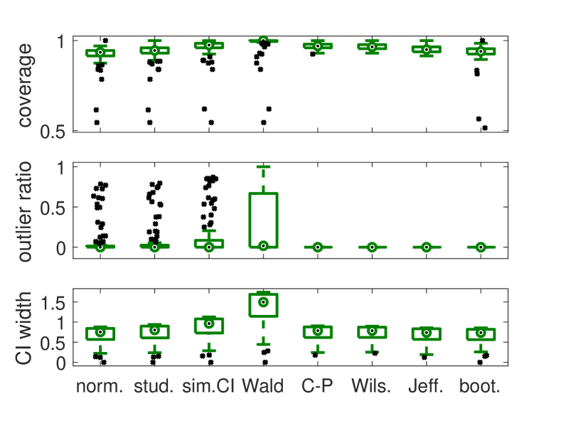
Figure 1: Binomial distribution. The test condition perspective considers the performance measures $\hat{M}_{x}$. We observe that for some estimators (norm., stud., sim.CI, Wald) there are several test conditions with bad properties (low coverage, high outlier ratio). The corresponding numbers are provided in Table II. Except for the Wald estimator, the binomial proportion estimators (C-P, Wils., Jeff.) work much better. Bootstrapping also leads to good results, but suffers from coverage outliers.

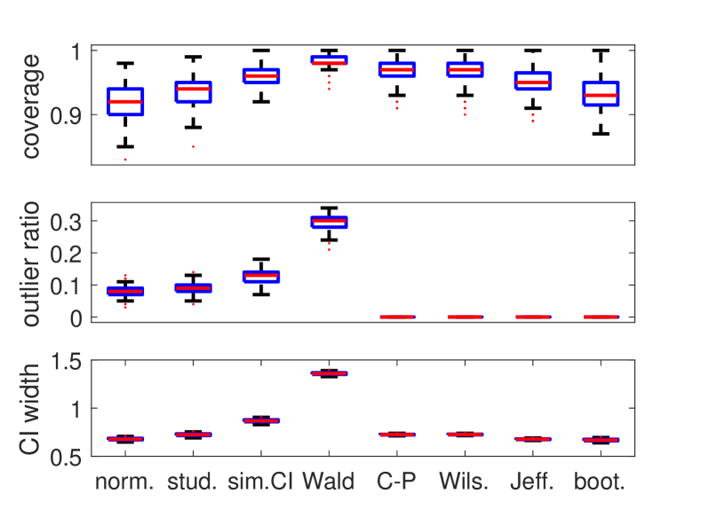
Figure 2: Binomial distribution. The QoE study perspective focuses on the performance measure $\hat{M}_{i}$. Hence, the performance (coverage, outlier ratio, CI width) is averaged over all test conditions within a single run. The boxplot summarizes then those average results $\hat{M}_{i}$ over all $r$ runs. Concrete numbers are provided in Table II.

TABLE II: The performance metrics are averaged and differentiated for coverage from test condition perspective ($\hat{C}_{i}$) and a QoE study perspective ($\hat{C}_{x}$) for the three scenarios. Minimum coverage is denoted by $\hat{C}_{x|i}^{m}$ and coverage outliers in the boxplot by $\hat{C}_{x|i}^{o}$.

Binomial	$\hat{C}$	$\hat{C}_{x}^{o}$	$\hat{C}_{x}^{m}$	$\hat{C}_{i}^{o}$	$\hat{C}_{i}^{m}$	$\hat{O}$	$\hat{W}$
norm.	0.92	0.08	0.55	0.01	0.83	0.08	0.68
stud.	0.93	0.09	0.55	0.01	0.85	0.09	0.72
sim.CI	0.96	0.08	0.55	0.00	0.92	0.13	0.87
Wald	0.98	0.14	0.55	0.04	0.94	0.30	1.36
C-P	0.97	0.01	0.93	0.03	0.91	0.00	0.72
Wils.	0.97	0.00	0.93	0.04	0.90	0.00	0.73
Jeff.	0.95	0.00	0.92	0.04	0.89	0.00	0.68
boot.	0.93	0.05	0.52	0.00	0.87	0.00	0.67
Low. var.	$\hat{C}$	$\hat{C}_{x}^{o}$	$\hat{C}_{x}^{m}$	$\hat{C}_{i}^{o}$	$\hat{C}_{i}^{m}$	$\hat{O}$	$\hat{W}$
norm.	0.90	0.10	0.28	0.00	0.82	0.00	0.48
stud.	0.91	0.09	0.28	0.00	0.83	0.00	0.51
sim.CI	0.93	0.10	0.28	0.01	0.87	0.00	0.61
Wald	1.00	0.00	1.00	0.00	1.00	0.00	1.67
C-P	1.00	0.23	0.98	0.14	0.99	0.00	0.87
Wils.	1.00	0.24	0.98	0.16	0.99	0.00	0.87
Jeff.	1.00	0.05	0.98	0.23	0.97	0.00	0.82
boot.	0.91	0.11	0.28	0.01	0.83	0.00	0.47

Figures 1 and 2 show the results for the binomial distribution scenario for the TC and QoE study perspective, respectively.

The boxplots shows the median within the box. The bottom and top of the box are the first and third quartiles. The upper and lower ends of the whiskers denotes the most extreme data point that is maximum and minimum 1.5 interquartile range (IQR) of the upper and lower quartile, respectively. Data outside 1.5 IQR are marked as outlier with a dot.

An overview on the performance measures is provided in Table II. The numerical results from the binomial case show that Clopper-Pearson, Jeffreys and bootstrapping have a good performance from the test condition and QoE study perspective. They have a good coverage, do not suffer from outliers, and have small CI widths.

The proposed idea based on binomial proportion fails if the distribution has a higher variance than a binomial distribution. Then, the coverage is poor; the confidence intervals are too small, as only binomial variances are assumed, but in reality we have higher variances. This is however very rare in actual QoE studies. If the variances are higher, this is often an indicator for hidden influence factors in the test setup or some other issues [7].

IV-D Low Variance Scenario

We only consider the QoE study perspective now which is provided in Figure 3. In case of low variances, the three identified estimators (Wilson, Clopper-Pearson, Jeffreys) still have a very good performance, and coverage is 100%. However in that case, the CI width is larger than for the normalized or student-t estimators. The reason for this is that the proposed estimators assume a binomial distribution (i.e., a much larger variance) and necessarily overestimate the CIs. For all estimators, the outlier ratio is zero. Still normalized or student-t have some problems to cover certain TCs at the edge (see $\hat{C}^{m}_{x}$ or $\hat{C}^{o}_{x}$).

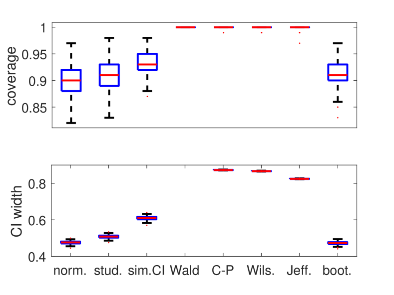
Figure 3: Low variance scenario. For all estimators, the outlier ratio is zero. Wald interval average CI width is about 1.67. The proposed binomial based CBI estimators lead to higher CIs than normalized estimators, as the assumed binomial distribution has a higher variance. Thus, the estimators are conservative for low variances.

Figure 4 considers the average CI width and coverage when varying the number $n$ of subjects in the study. The most efficient way to decrease the CI width is to increase $n$. It is worth to note that the binomial proportions estimators show almost constant coverage in contrast to bootstrapping.

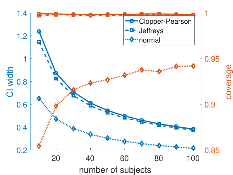
Figure 4: Low variance scenario. The average coverage $\hat{C}$ and CI width $\hat{W}$ are considered depending on the number of subjects of the study. The outlier ratio is zero for the three considered estimators.

V Recommendations and Conclusions

Subjective QoE studies often involve a relatively small number of test participants. Moreover, used rating scales are commonly discrete and bounded at both ends, with study results reported in the form of MOS values and CIs derived for various test conditions to quantify the significance of MOS values. Given the importance of using efficient CI estimators in the context of deriving QoE models, we evaluate several MOS CI estimators, and develop our own estimator based on binomial proportions. The numerical results indicate that the proposed idea based on binomial estimators is robust and conservative in practice. Wilson, Clopper-Pearson, and Jeffreys lead to comparable results, with excellent coverage and outlier properties. However, very good coverage comes along with costs of having larger CI widths. The Wald interval performs poorly, unless $n$ is quite large, which is not commonly the case in QoE studies. Standard confidence intervals based on normal and student-t distribution, as well as simultaneous CIs for multinomial distributions, suffer from the CIs exceeding the bounds of the rating scale. Bootstrapping has similar issues, i.e., some test conditions are not captured properly, but the outlier ratio is always zero due to sampling.

In summary, for QoE tests characterized by a small sample size and the use of discrete bounded rating scales, the proposed binomial estimators (Clopper-Pearson, Wilson, Jeffreys) are conservative, but exact and recommended. For decreasing the CI widths, bootstrapping or standard CI may be used in case of low variance (when the SOS parameter $a<0.1$) at the cost of decreased coverage – but the most effective way is to increase the number of subjects. If the SOS parameter is larger than for a binomial distribution ($a>\frac{1}{k-1}$), the results and test design should be checked, as there may be hidden influence factors in the study. An implementation of the CI estimators and the recommended estimators based on the SOS parameter is available in Github https://github.com/hossfeld.

References

- [1] S. M. Patrick Le Callet and A. Perkis, “Qualinet white paper on definitions of quality of experience,” European Network on Quality of Experience in Multimedia Systems and Services, Tech. Rep. Version 1.2, 2013.
- [2] T. Hoßfeld, P. E. Heegaard, M. Varela, and S. Möller, “Qoe beyond the mos: an in-depth look at qoe via better metrics and their relation to mos,” Quality and User Experience, vol. 1, no. 1, p. 2, 2016.
- [3] ITU-T, “Methods, metrics and procedures for statistical evaluation, qualification and comparison of objective quality prediction models,” International Telecommunication Union, Tech. Rep. P.1401, July 2012.
- [4] L. Janowski and M. Pinson, “Subject bias: Introducing a theoretical user model,” in Quality of Multimedia Experience (QoMEX), 2014 Sixth International Workshop on. IEEE, 2014, pp. 251–256.
- [5] ITU-T, “Methods for the subjective assessment of video quality, audio quality and audiovisual quality of internet video and distribution quality television in any environment,” International Telecommunication Union, Tech. Rep. P.913, March 2016.
- [6] S. Jin, Computing Exact Confidence Coefficients of Simultaneous Confidence Intervals for Multinomial Proportions and their Functions. Department of Statistics, Uppsala University, 2013.
- [7] T. Hoßfeld, R. Schatz, and S. Egger, “Sos: The mos is not enough!” in Quality of Multimedia Experience (QoMEX), 2011 Third International Workshop on. IEEE, 2011, pp. 131–136.
- [8] A. M. Pires and C. Amado, “Interval estimators for a binomial proportion: Comparison of twenty methods,” REVSTAT–Statistical Journal, vol. 6, no. 2, pp. 165–197, 2008.
- [9] S. E. Vollset, “Confidence intervals for a binomial proportion,” Statistics in medicine, vol. 12, no. 9, pp. 809–824, 1993.
- [10] L. D. Brown, T. T. Cai, and A. DasGupta, “Interval estimation for a binomial proportion,” Statistical science, pp. 101–117, 2001.
- [11] R. G. Newcombe, Confidence intervals for proportions and related measures of effect size. CRC Press, 2012.
- [12] A. Agresti and B. A. Coull, “Approximate is better than “exact” for interval estimation of binomial proportions,” The American Statistician, vol. 52, no. 2, pp. 119–126, 1998.
- [13] C. J. Clopper and E. S. Pearson, “The use of confidence or fiducial limits illustrated in the case of the binomial,” Biometrika, pp. 404–413, 1934.
- [14] H. Jeffreys, The theory of probability. OUP Oxford, 1998.
- [15] B. Efron, “Bootstrap methods: another look at the jackknife,” in Breakthroughs in statistics. Springer, 1992, pp. 569–593.