Sulphur chemistry in the L1544 pre-stellar core

Abstract

The L1544 pre-stellar core has been observed as part of the ASAI IRAM 30m Large Program as well as follow-up programs. These observations have revealed the chemical richness of the earliest phases of low-mass star-forming regions. In this paper we focus on the twenty-one sulphur bearing species (ions, isotopomers and deuteration) that have been detected in this spectral-survey through fifty one transitions: CS, CCS, C₃S, SO, SO₂, H₂CS, OCS, HSCN, NS, HCS⁺, NS⁺ and H₂S. We also report the tentative detection (4 $\sigma$ level) for methyl mercaptan (CH₃SH). LTE and non-LTE radiative transfer modelling have been performed and we used the nautilus chemical code updated with the most recent chemical network for sulphur to explain our observations. From the chemical modelling we expect a strong radial variation for the abundances of these species, which mostly are emitted in the external layer where non thermal desorption of other species has previously been observed. We show that the chemical study cannot be compared to what has been done for the TMC-1 dark cloud, where the abundance is supposed constant along the line of sight, and conclude that a strong sulphur depletion is necessary to fully reproduce our observations of the prototypical pre-stellar core L1544.

1 Introduction

Sulphur is the tenth most abundant element in our Galaxy and has been the subject of a lot of controversy over the past 20 years. Most observations of diffuse media (probing different conditions) find no elemental depletion of sulphur (e.g. Howk et al., 2006). With a detailed analysis, Jenkins (2009) seems to show a depletion with increasing density (as for the other elements) but discussed the possible observational bias of this result. On the contrary, only a small fraction of the cosmic sulphur abundance is seen in cold dense cores (through observable molecules such as SO and CS) (e.g. Tieftrunk et al., 1994; Palumbo et al., 1997). To reproduce these small abundances, chemical models need to deplete the elemental abundance of sulphur to "hide" the overflow of sulphur (see for example Wakelam et al., 2004). The explanation commonly proposed is that the missing sulphur is locked on the icy mantles of dust grains (e.g. Millar & Herbst, 1990; Ruffle et al., 1999). The controversy resides in the fact that, until now, only OCS (Geballe et al., 1985; Palumbo et al., 1995, 1997) and possibly SO₂ (Boogert et al., 1997; Zasowski et al., 2009) have been detected in solid state towards high-mass protostars, with abundances ($\sim$ 10^-7) less than 4% of the sulphur cosmic abundance. H₂S, the most likely natural product of hydrogenation of sulphur on grains, has not been detected and the upper limits on the abundance are $3\times 10^{-7}$ and $3\times 10^{-6}$ (assuming an abundance of H₂O in ices of $10^{-4}$) (Smith, 1991). The long standing question is then where is the sulphur that appears to be depleted from the gas phase in the dense regions of the interstellar medium?
Experimental measurements have been performed in order to understand which species are good candidates for sulphur in its solid state. OCS, for example, is formed by cosmic-ray irradiation, although it is easily destroyed on a long term (Garozzo et al., 2010). Ferrante et al. (2008) discussed the alternative of carbon disulphide (CS₂), which has been detected in the coma of comet 67P/Churyumov-Gerasimenko (Calmonte et al., 2016), although not detected in ices yet. Hydrated sulphuric acid (H₂SO₄) was also suggested by Scappini et al. (2003) as the main reservoir. Photoproducts of H₂S ice processing were proposed as a plausible explanation of the absence of H₂S in the ices and the sulphur depletion towards dense clouds and protostars (Jiménez-Escobar & Muñoz Caro, 2011). A large fraction of the missing sulphur in dense clouds could thus be polymeric sulphur residing in dust grains as proposed by Wakelam et al. (2004). Finally, Druard & Wakelam (2012) have proposed polysulphanes (H₂S_n) as possible carriers for sulphur on grains.

So far, only a few studies of sulphur chemistry have been performed in the cold regions of the interstellar medium. A sulphur depletion factor of $\sim$ 100 has been adopted to explain the chemistry in starless cores (Tafalla et al., 2006; Agúndez & Wakelam, 2013). A higher gas-phase sulfur abundance approaching the cosmic value of 1.5 $\times$ 10^-5 has been found in bipolar outflows (Bachiller & Pérez Gutiérrez, 1997; Anderson et al., 2013), photodissociation regions (Goicoechea et al., 2006), and hot cores (Esplugues et al., 2014). In these cases, this abundance was possibly interpreted by the release of the sulphur bearing species from the icy grain mantles because of thermal and non-thermal desorption and sputtering. Very recently, such a study has been done by Fuente et al. (2016) towards the Barnard B1b globule that hosts two candidates for the first hydrostatic core (FHSC). Their pointed position lies in between the two cores (B1b-N and B1b-S) leading to a difficult analysis. Their observational data are fitted using a chemical modelling with an elemental depletion of $\sim$ 25 for sulphur. Fuente et al. (2016) proposed that the low sulfur depletion and high abundances of complex molecules could be the result of two factors, both related to the star formation activity: the enhanced UV fields and the surrounding outflows. The star formation activity could also have induced a rapid collapse of the B1b core that preserves the high abundances of the sulphured species. In addition, the outflow associated with B1b-S may heat the surroundings and contribute to stop the depletion of S-molecules. More recently, Vidal et al. (2017) compared the observations of sulphur bearing species towards the TMC-1 (CP) dark cloud with the results from an updated chemical model and concluded that sulphur depletion is not required although a factor of three depletion also fitted the observations.

As part of the IRAM-30m Large Program ASAI (Lefloch et al., 2018), we carried out a highly sensitive, unbiased spectral survey of the molecular emission of the L1544 pre-stellar core with a high spectral resolution. In the present study we report on the detection of twenty-one sulphur bearing species in this core, use a radiative transfer modelling to determine the observed column densities and compare with the most up to date chemical modelling for sulphur chemistry.

We present in Section 2 the observations from the ASAI spectral survey and the line identification for the sulphur bearing species. Based on the detections and tentative detection, we compute in Section 3 the column densities of these species. We present in Section 4 the deuterium fraction, which is expected to be high in a pre-stellar core, and compare with their relative non sulphur bearing molecules. In Section 5, we use a detailed chemical modelling and confront the results with the observations.

2 Observations

The observations for all transitions quoted in Table 6 were performed at the IRAM-30m toward the dust peak emission of the L1544 pre-stellar core (${\rm\alpha_{2000}=05^{h}04^{m}17.21^{s},\delta_{2000}=25\degr 10\arcmin 42.8\arcsec}$) in the framework of the ASAI Large Program, except for H₂S which was observed as a follow-up project. Observations at frequencies lower than 80 GHz have been performed in December 2015. All the details of these observations can be found in Vastel et al. (2014) and Quénard et al. (2017b) and line intensities are expressed in units of main-beam brightness temperature.
The ortho–H₂S (1_1,0 – 1_0,1) at 168762.75 MHz has been observed with the IRAM-30m towards the dust peak emission on March 19 and 20, 2017, with the use of the spectral line Eight MIxer Receivers (EMIR) in band E150 combined with the narrow mode of the Fast Fourier Transform Spectrometers (FTS) allowing a spectral resolution of 50 kHz. We used the frequency switching observing mode with a frequency throw of 7.14 MHz, which allows a good removal of the ripples including standing waves between the secondary and the receivers (Fuente et al., 2016). Pointing was checked every 1.5 hour on the nearby continuum sources 0430+352, 0439+360 and 0316+413 with errors always within 3^′′. The system temperature was stable, at $\sim$ 230 K (2 mm of precipitable water vapour) resulting in an average rms of 9.1 mK for a resolution of 50 kHz. The IRAM beam varies from 33.5^′′ at 75 GHz to 23.9^′′ at 105 GHz and 15^′′ at 168 GHz.

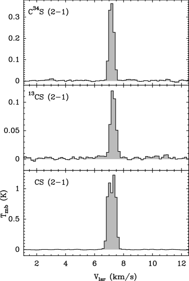
Figure 8: ¹²CS, ¹³CS and C³⁴S 2–1 detected line (in $\rm T_{mb}$).

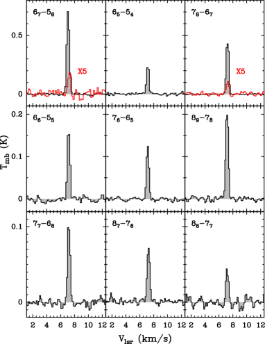
Figure 9: CCS (in black) and CC³⁴S (in red) detected lines (in $\rm T_{mb}$).

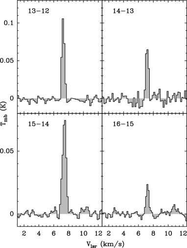
Figure 10: C₃S detected lines (in $\rm T_{mb}$).

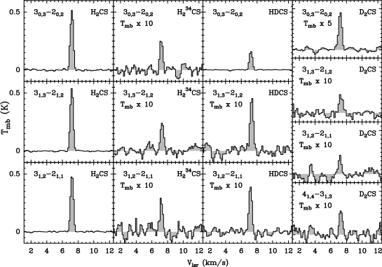
Figure 12: H₂CS, H₂³⁴CS, HDCS and D₂CS detected lines (in $\rm T_{mb}$).

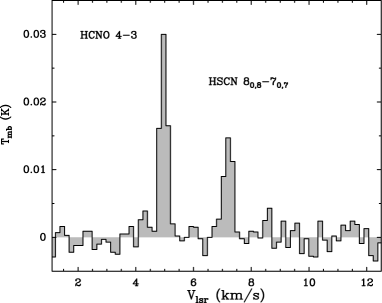
Figure 13: HSCN detected line (in $\rm T_{mb}$).

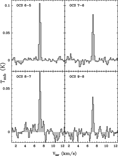
Figure 14: OCS detected lines (in $\rm T_{mb}$).

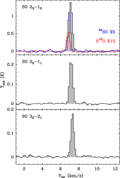
Figure 15: SO, S¹⁸O and ³⁴SO detected lines (in $\rm T_{mb}$).

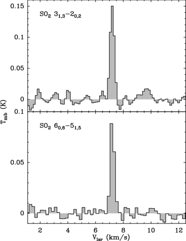
Figure 16: SO₂ detected lines (in $\rm T_{mb}$).

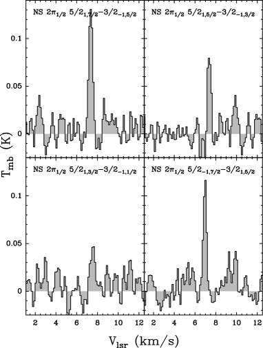
Figure 17: NS detected lines (in $\rm T_{mb}$).

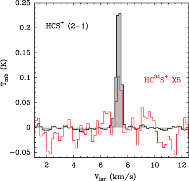
Figure 18: HCS⁺ (black) and HC³⁴S (red) 2–1 detected line (in $\rm T_{mb}$).

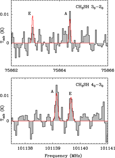
Figure 19: Tentative detection of CH₃SH. The LTE model ($\rm T_{ex}$ = 10K, N = 2.5 $\times$ 10¹¹ cm^-2, fwhm = 0.3 km/s) is over-plotted in red. The lines are in $\rm T_{mb}$.

Twenty-one sulphur bearing species have been detected in total and are shown in Appendix A: CS, ¹³CS and C³⁴S (Fig. 8), CCS and CC³⁴S (Fig. 9), C₃S (Fig. 10), H₂S (Fig. 11), H₂CS, H₂C³⁴S, HDCS and D₂CS (Fig. 12), HSCN (Fig. 13), OCS (Fig. 14), SO, S¹⁸O and ³⁴SO (Fig. 15), SO₂ (Fig. 16), NS (Fig. 17), NS⁺ (Cernicharo et al., 2018), HCS⁺ and HC³⁴S⁺(Fig. 18). We present, in Table 6, the spectroscopic parameters of the transitions detected using the CDMS (Müller et al., 2005) for most species except CC³⁴S for which we used JPL (Pickett et al., 1998). The line identification and analysis have been performed using the cassis software (Vastel et al., 2015). The results from the line fitting take into account the statistical uncertainties accounting for the rms (estimated over a range of 15 km s^-1 for a spectral resolution of 50 kHz). We also report a tentative detection (4 $\sigma$ level) for methyl mercaptan (CH₃SH) in Fig. 19.

3 Determination of the column densities

In this section we determine the column densities (or some upper limits) for the detected species. Different methods are used, depending on the number of detected transitions for each species, and also depending on the availability of collisional coefficients. These methods take into account the uncertainties based on the line fitting and also the absolute calibration accuracy, around 10$\%$ or better depending on the band considered. For species where multiple transitions have been detected, covering a wide range in energy, the rotational diagram method (see Fig. 1 in the case of CCS) is a useful tool to derive parameters such as the column density and excitation temperature. We performed this analysis for CCS, C₃S, H₂CS, H₂C³⁴S, HDCS, D₂CS, OCS and SO (see Table 1). When multiple transitions are detected we can also use a MCMC (Markov Chain Monte Carlo) method implemented within cassis. The MCMC method is an iterative process that goes through all of the parameters with a random walk and heads into the solutions space and the final solution is given by a $\chi^{2}$ minimization. All parameters such as column density, excitation temperature (or kinetic temperature and H₂ density in the case of a non-LTE analysis), source size, linewidth, V_lsr, can be varied. The partition functions have been computed in cassis for temperatures lower than 9.375 K which is the lowest temperature given by the CDMS database for some species. These are computed as:

$$Q(T)=\sum_{i}g_{i}\times exp(-E_{i}/kT)$$ (1)

where g_i and E_i are the statistical weight and energy, respectively, of the i level. Table 1 shows the results from the MCMC method for a LTE analysis. Note that the emission is compatible with a source size larger than the IRAM beam of $\sim$ 30^′′.

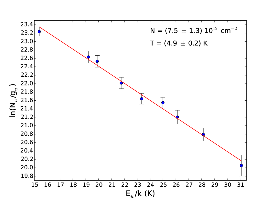
Figure 1: Rotational diagram analysis for the nine detected transitions of CCS. The CCS column density and rotational temperature are quoted in the upper right corner.

Table 1: Temperature and column density of sulphur species in L1544, under the LTE condition, using MCMC and rotational diagram analysis.

	MCMC				Rotational diagram
Species	$\rm T_{ex}$	N	FWHM	$\rm V_{lsr}$	$\rm T_{rot}$	N
	(K)	(cm-2)	(km s-1)	(km s-1)	(K)	(cm${}^{-2})$
CCS	$5.6\pm 0.2$	$6.5(\pm 0.9)$ x $10^{12}$	$0.40\pm 0.01$	$7.18\pm 0.01$	$4.9\pm 0.2$	$7.5(\pm 1.3)$ x $10^{12}$
C3S	$6.2\pm 0.5$	$3.1(\pm 0.1)$ x $10^{12}$	$0.42\pm 0.01$	$7.22\pm 0.01$	$7.9\pm 0.2$	$8.8(\pm 0.7)$ x $10^{11}$
H2C34S	$14.1\pm 2.0$	$3.5(\pm 0.7)$ x $10^{11}$	$0.43\pm 0.03$	$7.24\pm 0.02$	$14.6\pm 0.8$	$3.1(\pm 0.2)$ x $10^{11}$
D2CS	$9.6\pm 1.5$	$1.1(\pm 0.7)$ x $10^{12}$	$0.47\pm 0.02$	$7.22\pm 0.01$	$10.8\pm 0.8$	$6.5(\pm 0.6)$ x $10^{11}$
OCS	$7.5\pm 0.6$	$6.3(\pm 1.6)$ x $10^{12}$	$0.36\pm 0.01$	$7.18\pm 0.01$	$8.8\pm 0.2$	$4.1(\pm 0.2)$ x $10^{12}$
HDCS	$6.8\pm 0.6$	$1.6(\pm 0.8)$ x $10^{12}$	$0.42\pm 0.01$	$7.23\pm 0.01$	$7.5\pm 0.5$	$8.4(\pm 1.1)$ x $10^{11}$
H2CS	$12.3\pm 0.7$	$7.3(\pm 1.0)$ x $10^{12}$	$0.41\pm 0.01$	$7.20\pm 0.01$	$13.1\pm 0.9$	$5.8(\pm 0.6)$ x $10^{12}$
SO	$9.7\pm 1.8$	$5.2(\pm 0.8)$ x $10^{12}$	$0.34\pm 0.01$	$7.22\pm 0.01$	$7.9\pm 1.6$	$7.2(\pm 3.2)$ x $10^{12}$

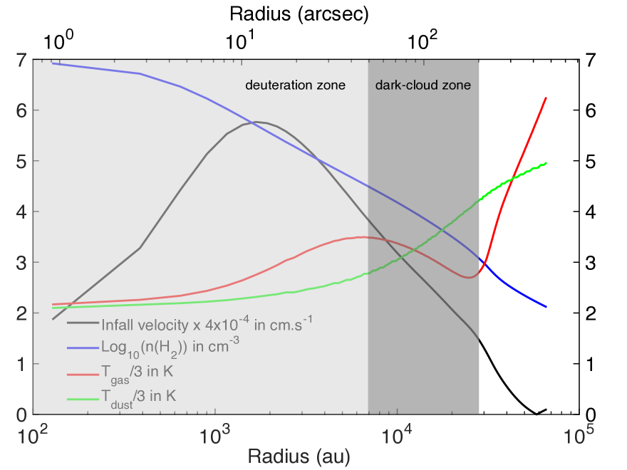
Figure 2: Gas and dust temperature, density, and velocity profiles of the L1544 pre-stellar core as a function of the radius in arcseconds and au from Keto et al. (2014).

The computed column densities and temperatures shown in Table 1 show similar results, especially in the case of CCS for which we have nine transitions detected. Some differences occur when the number of transitions decreases. For example, there is a factor of two on the computation of the column density of HDCS (and a factor of three for C₃S) between both methods, reflecting the low number of transitions detected covering a small range in energy E_u = 8.9, 17.7, 18.1 K (E_u = 25.3, 29.1, 33.3, 33.7 K for C₃S). The rotational diagram analysis cannot be performed on species for which only a few transitions are detected. For these species, we fixed the excitation temperature at 10 K, which is the average kinetic temperature of the L1544 core in the IRAM beam (see Fig. 2), or slightly varied the temperature to be compatible with the non detected transitions in our spectral survey, and constrained their column density by adjusting the spectra. The resulting column densities are given in Table 2 as N_species. We present in Fig. 19 the tentative detection for methyl mercaptan (CH₃SH) in our spectral survey, convincingly reinforced by a LTE modelling (in red) with a strong upper limit on the column density of $2.5\times 10^{11}cm^{-2}$ using a fixed temperature of 10 K, a full width at half maximum of 0.3 km/s, a velocity in the standard of rest of 7.1 km/s. Note that varying the excitation temperature from 8 to 12 K for these species does not significantly change the results.

Table 2: Derived column density (N) with a fixed excitation temperature of 10 K for species where one or two transitions have been detected or with a varied excitation temperature so that the LTE modelling is compatible with the non detected transitions in our spectral survey.

Species	$\rm T_{ex}$	$\rm N_{species}$	$\rm N_{main\,isotopologue}$
	(K)	(cm-2)	(cm-2)
HCS+	$10$	$(6.2-6.5)\times 10^{11}$
HC34S+	$10$	$(4.8-5.2)\times 10^{10}$	$(1.1-1.2)\times 10^{12}$
CS	$10$	$(4.0-4.4)\times 10^{12}$
13CS	$10$	$(2.6-3.0)\times 10^{11}$	$(1.8-2.0)\times 10^{13}$
C34S	10	$(7.8-8.3)\times 10^{11}$	$(1.8-2.0)\times 10^{13}$
CC34S	6–7	$(4-6)\times 10^{11}$	$(0.9-1.4)\times 10^{13}$
HSCN	$10$	$(5.8-6.2)\times 10^{10}$
NS	$10$	$(1.4-1.6)\times 10^{12}$
34SO	5–6	$(1.3-1.6)\times 10^{12}$	$(3.0-3.6)\times 10^{13}$
S18O	6–8	$(3-3.2)\times 10^{11}$	$(1.7-1.8)\times 10^{14}$
CH3SH	10	$\leq 2.5\times 10^{11}$

For OCS, SO and SO₂ we carried out a non-LTE analysis using the LVG (Large Velocity Gradient) code by Ceccarelli et al. (2003), using the collision rates by Green & Chapman (1978), Lique et al. (2007) and Cernicharo et al. (2011) respectively. Table 3 lists the results (H₂ density, kinetic temperature and column density) from the LVG analysis, taking into account the observed integrated fluxes and the corresponding rms (see Table 6). These species are likely emitted in the external layer where the density is lower and the temperature is higher than in the center where $\rm T_{gas}\sim T_{dust}$ $\sim$ 7 K and n(H₂) $\sim$ 10⁷ cm^-3 (see Fig. 2). Note also that the emission is compatible with a source size larger than the maximum IRAM beam of $\sim$ 30^′′. For NS⁺, we used the column density derived from Cernicharo et al. (2018): 2.3 $\times$ 10¹⁰ cm^-2.
The H₂S transition is the only transition among our sulphur bearing species that presents a double-peaked profile that cannot simply be analysed in LTE (see Fig. 11). We estimated a lower limit on the H₂S column density of 1.6 $\times$ 10¹² cm^-2, from a simple LTE modelling using an excitation temperature of 10 K and we use this limit in section 5 (see Fig. 4) as a comparison for the chemical modelling. We also use, in Appendix B, the variation of H₂S abundance as a function of radius (from section 5) combined with a 3D radiative transfer treatment to try to reproduce the line profile, taking into account the density and temperature profiles as well as the velocity profile of the L1544 pre-stellar core.

Table 3: Results from the non-LTE analysis for the OCS, SO and SO₂ species.

Species	$\rm n_{H_{2}}$	$\rm T_{K}$	$\rm N$
	(cm-3)	(K)	(cm-2)
OCS	(7 $\pm$ 3.0) $\times$ $10^{3}$	13 $\pm$ 2	4 ($\pm$ 1) $\times 10^{12}$
SO	(2 $\pm$ 1) $\times$ $10^{4}$	$\geq$ 12	$\geq$ 8 $\times$ $10^{12}$
SO2	(2 $\pm$ 1) $\times$ $10^{4}$	12 $\pm$ 1	(2.0–3.5) $\times$ $10^{12}$

Isotopologues may be used when transitions are optically thick. We decided to use the isotopologues of the more abundant species presented in Section 2 to refine some of the column densities determined earlier. For example, one transition for ¹²CS, ¹³CS and C³⁴S have been detected in our spectral survey. A simple LTE analysis gives a ¹²CS/¹³CS ratio between 13.3 and 16.9, much below the value of 68 determined in the local interstellar medium (Milam et al., 2005; Asplund et al., 2009; Manfroid et al., 2009) for ¹²C/¹³C. The ¹²CS (2–1) is likely optically thick and hinders the determination of the true column density for ¹²CS. Using ¹³CS and a ¹²C/¹³C ratio of 68, we obtain a value of N(¹²CS)=(1.77–2.04) $\times$ 10¹³ cm^-2. The same analysis can be also applied for ³⁴S/³²S. The LTE analysis for C³⁴S gives a C³⁴S/C³²S ratio of $\sim$ 0.2, much higher than the value (0.044) in the vicinity of the Sun (Chin et al., 1996). The CS column density derived from C³⁴S gives (1.77–1.89) $\times$ 10¹³ cm^-2, similar to the value derived from ¹³CS. Previous observations of the CS (2–1) double peaked line profile, as well as a map over the whole core, have shown that CS is depleted in the central positions (Tafalla et al., 2002; Hirota et al., 1998). Aikawa et al. (2003) used these observations to compute the column density from their best-fit model assuming a spherical core with radius of 15000 au. Using the collision coefficients for para-H₂ from Green & Chapman (1978), the resulting column density for the CS molecule is 4.6 $\times$ 10¹³ cm^-2 (with an uncertainty factor of 2–3), a factor 10 higher than their LTE value, but compatible with our LTE computation using ¹³CS and ¹²CS/¹³CS=68. The ³⁴S/³²S ratio for both HCS⁺ and CCS are compatible with the value found in the vicinity of the Sun. For the SO molecule, two isotopologues have been detected: ³⁴SO and S¹⁸O. The respective SO column densities based on the local values of the isotopic ratios are $\sim$ 3.2 $\times$ 10¹³ and $\sim$ 1.8 $\times$ 10¹⁴ cm^-2 respectively, compatible with the lower limit (8 $\times$ 10¹² cm^-2) found using a non-LTE formalism (see Table 3).
We present in the fourth column of Table 2, the column density (as $\rm N_{main\,isotopologue}$) of the main species based on the rarer isotopologue column density and using ¹²C/¹³C, ³²S/³⁴S and ¹⁶O/¹⁸O ratios of 68, 23, and 557 (Wilson, 1999) respectively. CS and HCS⁺ are the only species where optical depth affects the determination of the column densities and we will use their values, determined from the rare isotopologues (¹³CS, C³⁴S and HC³⁴S⁺), when comparing with the outcome of the chemical model described in Section 5.
Very recently, the thioformyl radical (HCS) and its metastable isomer HSC have been detected toward the molecular cloud L483 (Agúndez et al., 2018). These species have not been detected in our spectral survey, and we can estimate an upper limit on the column density for both species, using an excitation temperature of 10K: N(HCS) $\leq$ 3 $\times$ 10¹² cm^-2 and N(HSC) $\leq$ 6 $\times$ 10¹⁰ cm^-2, a factor two to three lower than those derived towards L483.
Table 4 summarizes the column densities that have been computed in this Section which will be used in Section 5.

4 Deuterium Fraction of the sulphur bearing species

An extreme molecular deuteration is a major characteristic of pre-stellar cores. Although the deuterium abundance is about 1.5 $\times$ 10^-5 relative to hydrogen (Linsky 2003), singly, doubly and even triply deuterated molecules have been detected with D/H ratios reaching 100$\%$ (see Ceccarelli et al., 2014, for a review). Deuterium fractionation occurs in the cold and dense regions of the interstellar medium where CO is depleted from the gas phase, which leads to the preferential reactions between the H₃⁺ ion with HD, feeding the deuterium of the latter ion, and distributing deuterium in the gas-phase and on the grain surfaces. In those regions where CO is highly depleted and H₂ is mostly in para form, the abundance of D₂H⁺ should be similar to that of H₂D⁺ (Roberts et al., 2003). This was confirmed with the detection of D₂H⁺ toward the pre-stellar core 16293E (Vastel et al., 2004). A high deuterium fractionation has already been detected in L1544 (e.g. Caselli et al., 1999; Crapsi et al., 2005; Bizzocchi et al., 2014) in which H₂D⁺ has been detected (Caselli et al., 2003). The central 7000 au is called the deuteration zone (see Fig. 2), where the freeze-out of abundant neutrals such as CO and O, the main destruction partners of the H₃⁺ isotopologues, favour the formation of deuterated molecules. The outer ring (7000–30000 au), is called the dark-cloud zone (Caselli et al., 2012; Ceccarelli et al., 2014), where the carbon is mostly locked in CO, gas-phase chemistry is regulated by ion-molecule reactions and deuterium fractionation is reduced.
From Table 1 we can compute the following fractionation ratios: H₂C³⁴S/H₂CS = 0.048 $\pm$ 0.016, HDCS/H₂CS = 0.219 $\pm$ 0.140 and D₂CS/H₂CS = 0.151 $\pm$ 0.117. The first one is compatible with the ³⁴S/³²S ratio of 0.044 in the vicinity of the Sun (Chin et al., 1996) which means that the H₂CS detected transitions are optically thin and give a good estimate of the total column density of H₂CS. The deuteration fractionation ratios for singly and doubly deuterated thioformaldehyde are both comparable and present an extremely high D enhancement. As a comparison, for the B1 cloud, the derived HDCS/H₂CS and D₂CS/H₂CS abundance ratios are 0.33 and 0.11 respectively (Marcelino et al., 2005).
At the high densities and very low temperatures found in pre-stellar cores, D₂CO forms efficiently (Tielens, 1983) because of its lower zero energy level compared to that of H₂CO, through gas chemistry where deuterium is passed from the deuterated forms of H${}_{3}^{+}$ and CH${}_{3}^{+}$ (Roberts et al., 2003, 2007). Considering the high densities in the central regions of L1544 where deuteration is the highest (see Fig. 2), the LTE assumption should be correct for the determination of the column densities of the deuterated species, as found in the case of B1 (Marcelino et al., 2005). The collision coefficients are unkown for the D₂CS and HDCS species, but assuming a typical range of 10^-11–10^-10 cm³ s^-1 and using Einstein coefficients of $\sim$ 10^-5 s^-1(see Table 6), we can estimate critical densities between 10⁵ and 10⁶ cm^-3. These values correspond to the densities found at 4 $\times$ 10³ and 10³ au respectively from the L1544 center (see Fig. 2) and are higher than densities found at larger distances. Therefore, it is reasonable to assume that LTE conditions are valid for the gas in the deuteration zone, whereas the emission from the outer gas is likely sub-thermal.
The formation of the deuterated forms of thioformaldehyde and formaldehyde should be similar (CO and CS being strongly depleted: Tafalla et al., 2002) and their deuterated ratios comparable. A map of formaldehyde and its deuterated counterparts has recently been performed by Chacòn-Tanarro et al. (submitted to A&A) in L1544 and they measured the following deuterated fractions at the dust peak where CO is heavily depleted (Caselli et al., 1999): D₂CO/H₂CO = 0.04 $\pm$ 0.03, HDCO/H₂CO = 0.03 $\pm$ 0.02. The derivation was done assuming optically thin emission and LTE, using a constant excitation temperature of 7 K (from the modelling of H₂CO). It is difficult to compare the deuterated fractions of both formaldehyde and thioformaldehyde because of the large error bars found for the latter. Overall, it seems that deuteration is somewhat more efficient for thioformaldehyde than for formaldehyde.

5 Evidence for sulphur depletion: a comparison between the observations and the chemical modelling

We now confront the results from the radiative transfer modelling presented in section 3 with the output of a detailed chemical modelling. The sulphur chemical network has recently been enhanced by Vidal et al. (2017), using experimental and theoretical rates and branching ratios from the literature. Basically, they added 46 sulphur bearing species along with 478 reactions in the gas-phase, 305 reactions on the grain surface and 147 reactions in the grain bulk. They tested the effect for this updated network on the output of a gas-grain chemical model for dark clouds conditions, with different elemental sulphur abundances. Their results show that, depending on the age of the observed cloud, the sulphur reservoir could be either atomic sulphur in the gas phase or HS/H₂S in icy grain bulks. From the chemical modelling, they conclude that depletion of sulphur is not required to explain the observations of the TMC-1 dark cloud. This cloud is at an earlier stage than L1544, and presents a constant density ($\sim$ 10⁴ cm^-3) and temperature ($\sim$ 10 K).
We used the same chemical network for our study combined with three-phases modellings, which allows to follow the evolution of chemical abundances for a given set of chemical and physical parameters. Gas-phase, grain surface and grain bulk chemistries are taken into account, along with exchanges between those phases: adsorption of gas-phase species onto the grain surfaces, thermal and non-thermal desorption of species from the grain surface into the gas-phase, and finally the exchange of species between the bulk and the surface of the grains. More details on the three-phase model can be found in Ruaud et al. (2016) and Vidal et al. (2017). We present in Fig. 3 the most critical reactions linking the sulphur bearing species that we detected (blue ellipses), but also the intermediate undetected species (purple boxes) and the reactions exchanges: blue arrows are for surface reactions, green arrows for electronic recombination and red arrows for bimolecular reactions. We used the nautilus’ outputs for the many models considered and extracted the main reactions leading to the production of the detected sulphur bearing species in L1544. These reactions are based on the KInetic Database for Astrochemistry (KIDA) (http://kida.obs.u-bordeaux1.fr/).

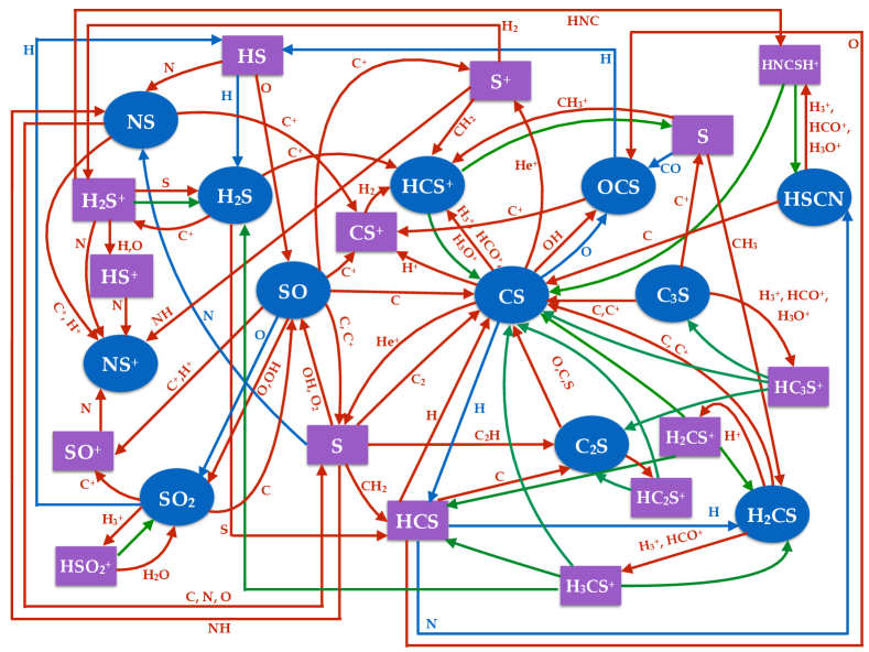
Figure 3: Simplified sulphur network. The blue ellipses being the detected species in L1544, the purple boxes being the intermediate undetected species, blue arrows are the surface reactions, green arrows the electronic recombination and red arrows the bimolecular reactions.

We have used the gas-grain chemical code nautilus in its three-phase model (gas phase, grain surface and mantle) to predict the abundances of all sulphur species in the cold core. We have already used nautilus in previous studies of the chemistry involved in the cold core (Quénard et al., 2017b; Vastel et al., 2018) and we follow here a similar method to stay consistent with these works. In the work led by Vidal et al. (2017), they considered a one-step chemical modelling with a constant density and temperature to model the physical conditions in TMC-1. Indeed, TMC-1 is a younger core than L1544 and the latter presents a density, temperature and velocity structure with evidence of gravitational contraction (Caselli et al., 2012; Keto et al., 2014). To take into account this structure, we therefore used a two-step model: the first phase represents the evolution of the chemistry in a diffuse or molecular cloud, with T = 20 K and several densities, ranging from 10² to 2 $\times$ 10⁴ cm^-3, depending on the model considered (see Quénard et al., 2017b; Vastel et al., 2018, for more details). The initial abundances considered are those labelled as "EA1" in Quénard et al. (2017b) and we only vary the sulphur atomic abundance (see below and Table 5). We follow the chemistry in this phase during 10⁶ years. We have checked that a variation of this age to 10⁵, 5 $\times$ 10⁶ or 10⁷ years does not change the resulting column densities by more than a factor 1.5. In order to compare the results from the chemical modelling (abundances with respect to H) with the observations (column density) of sulphur bearing molecules in L1544, we took into account the density profile across the core (see Quénard et al., 2017b) to determine the column density from the chemical modelling instead of the abundance:

$$N(X)=2\times\sum_{i=2}^{n}(r_{i-1}-r_{i})\times\frac{n(H)_{i-1}[X]_{i-1}+n(H)_{i}[X]_{i}}{2}$$ (2)

where r is the radius from the center for every layer, n(H)_i the gas density and [X]_i the abundance at radius r_i. The different N(X) are then weigthed using a Gaussian function with a FWHM depending on the beam of the IRAM 30m telescope (between 15^′′ and 30^′′, depending on the frequency) to compare with the observations. This procedure was not adopted in the case of TMC-1 for which a constant density profile has been used. In the case of L1544, we cannot simply divide the observed column density by the total H₂ column density since the emission is not radially constant.

Table 4: Column densities used for the comparison with the chemical modelling.

Species	N	method
	(cm-2)
CCS	(0.9–1.4) $\times$ 1013	CC34S
C3S	3.1 ($\pm$ 0.1) $\times$ 1012	MCMC
SO2	(2.0–3.5) $\times$ 1012	LVG
CS	(1.8–2.0) $\times$ 1013	13CS, C34S
OCS	4 ($\pm$ 1) $\times$ 1012	LVG
H2CS	7.3 ($\pm$ 1.0) $\times$ 1012	MCMC
HSCN	(5.8–6.2) $\times$ 1010	LTE
NS	(1.4–1.6) $\times$ 1012	LTE
NS+	2.3 $\times$ 1010	Cernicharo et al. (2018)
HCS+	(1.1–1.2) $\times$ 1012	HC34S+
SO	$\geq$ 8 $\times$ 1012	LVG
H2S	$\geq$ 1.6 $\times$ 1012	LTE
CH3SH	$\leq$ 2.5 $\times$ 1011	LTE

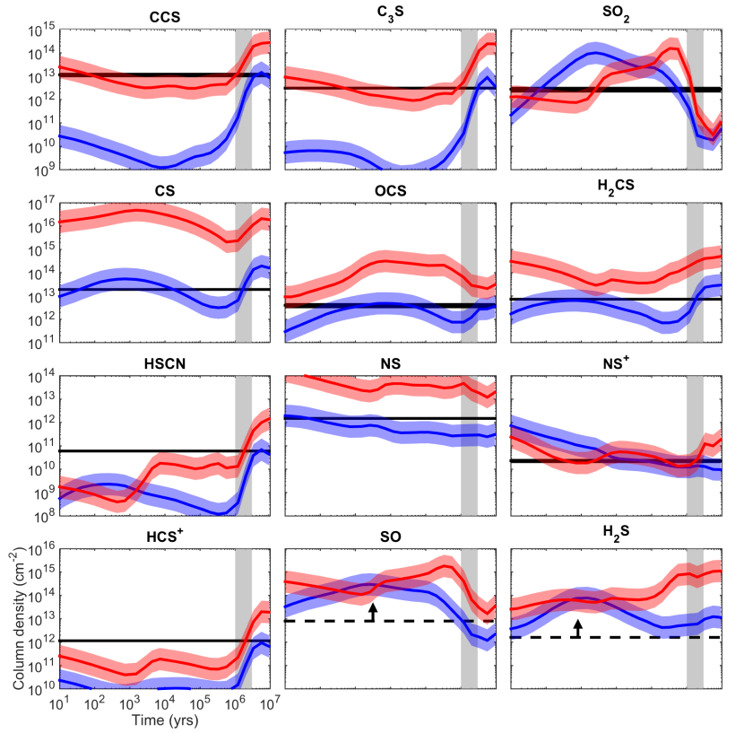
Figure 22: Variation of the modelled column density as a function of time and the comparison with the observed column density (black horizontal line). The blue lines correspond to model 2 (sulphur depletion: S/H=$8~{}10^{-8}$) and the red ones correspond to model 5 (sulphur non depletion: S/H=$1.5~{}10^{-5}$) as shown in Table 5. The thickness of the black line corresponds to the error bar of the observed column densities. A variation by a factor of three of modelled column densities is shown in corresponding coloured areas. The dashed black horizontal line for SO and H₂S correspond to the lower limit on the computation of the total column density. The gray vertical area highlights an age between [1–3] $\times$ 10⁶ years (see text).

We present in Fig. 4 the variation of the modelled column density as a function of time from nautilus and the comparison with the observed column density (black horizontal line). We use in Fig. 4 (black horizontal lines) the observed column densities from Table 4 that have been computed in Section 3 for the 13 sulphur bearing species. The width of the line represents the errors quoted in Table 4. The blue lines correspond to model 1 (sulphur depletion: S/H=8.0 $\times$ 10^-8) and the red ones correspond to model 4 (sulphur non depletion: S/H=1.5 $\times$ 10^-5) for an initial H density of 10² cm^-3. Table 5 shows the different modelling varying density in the first phase and the element gas phase abundances. From Fig. 4 we can clearly identify which model better reproduces the observations. A sulphur depletion seems necessary overall, with the exception of SO₂, although still within the error bars. Additional modelling are presented in Appendix C: Fig. 22 (initial H density of 3 $\times$ 10³ cm^-3, see Table 5) and 23 (initial H density of 2 $\times$ 10⁴ cm^-3, see Table 5).

Table 5: Chemical modelling parameters used for the first phase model.

Model	Density	Sulphur elemental
number	(cm-3)	abundance
1	$1\times 10^{2}$	$8.0\times 10^{-8}$
2	$3\times 10^{3}$	$8.0\times 10^{-8}$
3	$2\times 10^{4}$	$8.0\times 10^{-8}$
4	$1\times 10^{2}$	$1.5\times 10^{-5}$
5	$3\times 10^{3}$	$1.5\times 10^{-5}$
6	$2\times 10^{4}$	$1.5\times 10^{-5}$

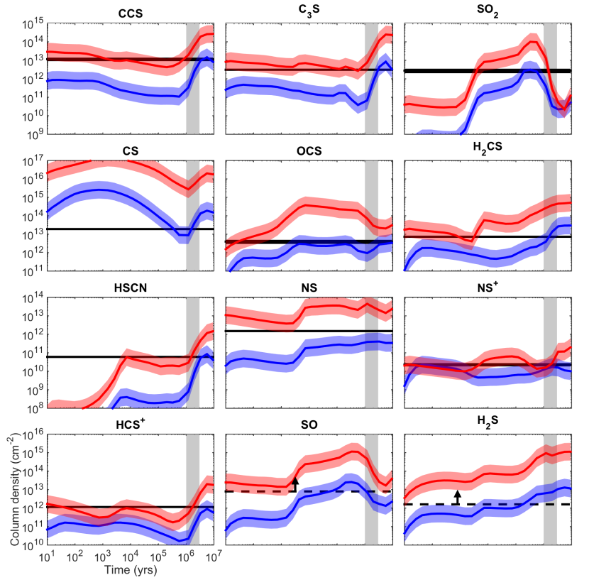
Figure 4: Variation of the modelled column density as a function of time and the comparison with the observed column density (black horizontal line). The blue lines correspond to model 1 (sulphur depletion: S/H=$8~{}10^{-8}$) and the red ones correspond to model 4 (sulphur non depletion: S/H=$1.5~{}10^{-5}$) as shown in Table 5. The thickness of the black line corresponds to the error bar of the observed column densities. A variation by a factor of three of modelled column densities is shown in corresponding coloured areas. The dashed black horizontal line for SO and H₂S correspond to the lower limit on the computation of the total column density. The gray vertical area highlights an age between [1–3] $\times$ 10⁶ years (see text).

Then, in order to find the "best-fit" model, we used the distance of disagreement computation (see for example Wakelam et al., 2006), applied on the column density, which is computed as follows:

$$D(t)=\frac{1}{n_{obs}}\sum_{i}|log(N(X))_{obs,i}-log(N(X))_{i}(t)|$$ (3)

where N(X)_obs,i is the observed column density, N(X)_i(t) is the modelled column density at a specific age and n_obs is the total number of observed species considered in this computation (10 in the case of non deuterated sulphur bearing species detected in L1544). Note that we did not take into account species where a lower limit has been derived from the observations (SO and H₂S) and an upper limit has been derived (CH₃SH). Fig. 5 shows the distance of disagreement for all 6 models explained in Table 5.
The minimum of the D(t) function is then obtained for the "best fit" age. Fig. 5 shows that 1) the "best-fit" age is 10⁶-10⁷ years for most models, compatible with previous estimates of the cloud age (Quénard et al., 2017b) and 2) the models where sulphur is depleted (models 1–3, respectively in red, yellow and green) are more favourable than models where sulphur is not depleted (models 4–6, respectively in light blue, dark blue and magenta). Moreover, the best solution for models 4 and 5 is found at very early age ($\sim$ 10³ years), which is not compatible with the age of the object. We report the best-fit age in Fig. 4 as a gray vertical area which highlights an age between [1–3] $\times 10^{6}$ years for a direct comparison between observations and modelling. The ten sulphur-bearing species are reproduced by the chemical model, within the observed error bars and considering a conservative factor of three to the modelled column densities. We are also in good agreement with the lower limits found for SO and H₂S. We present in Fig. 6 the radial distribution for all the detected sulphur bearing species in the network from Vidal et al. (2017), for an age between 10⁶ et 3 $\times$ 10⁶ years, compatible with the results from the distance of disagreement. The abundances clearly peak at a radius between [1-2] $\times$ 10⁴ au. Carbon, oxygen and sulphur depletion affect the cold and dense regions within L1544 (e.g. Vasyunin et al., 2017). Species like CO and CS disappear rapidly from the gas phase in the deuteration zone (see section 4), while species like N₂H⁺ and NH₃ survive much longer at high densities. As a result, the pre-stellar core gradually develops a differentiated interior characterised by a centre rich in depletion-resistant species (such as the deuterium bearing species) surrounded by layers richer in depletion-sensitive molecules (such as the sulphur bearing species). This molecular differentiation as been identified in many starless cores (e.g. Tafalla et al., 2006) and non-thermal desorption processes have been invoked (e.g. Vastel et al., 2014; Balucani et al., 2015; Vastel et al., 2016; Vasyunin et al., 2017): FUV photo-desorption, cosmic-rays and chemical desorption. As a consequence, we cannot simply assume a constant abundance as was assumed in dark clouds such as TMC-1 (Vidal et al., 2017) for the comparison between the observations and the chemical modelling. Note that in the current model, FUV photo-desorption plays a minor role as compared to the chemical desorption.

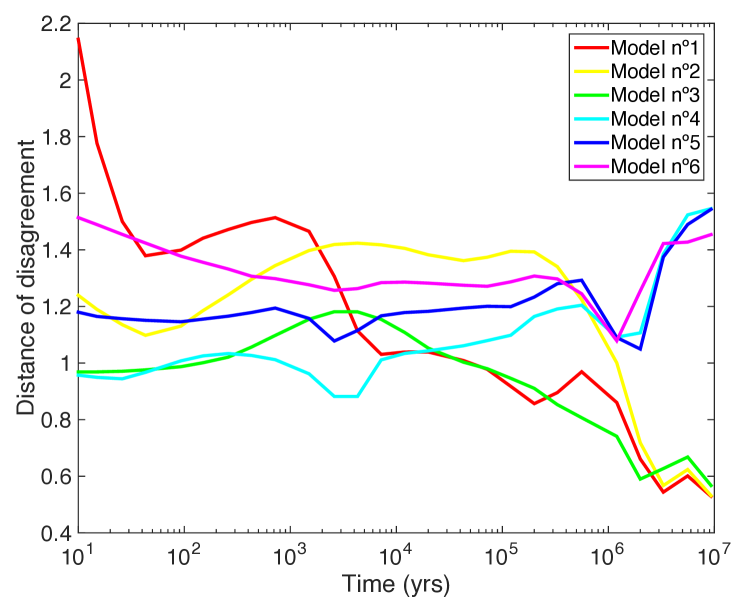
Figure 5: Distance of disagreement for models 1–3 (depletion) and 4–6 (non depletion). See Table 5.

Figure 6: Radial distribution of the detected sulphur bearing species abundances in L1544 for an age between 10⁶ and 3 $\times$ 10⁶ years, for models 1–6 (see Table 5).

Methyl mercaptan (CH₃SH) is tentatively detected in the L1544 pre-stellar core. It is likely emitted in the external layer of L1544 at $\sim$ 10⁴ au (see Fig. 7) where the density drops to about 10⁴ cm^-3 and the temperature increases to 10–12 K. We used the same chemical modelling as for the other sulphur-bearing species and present in Fig. 7 the results from the modelling for models 1–6 (see Table 5) compared to the upper limit on the column density (dashed line). It is clear from this Figure that a non-depletion regime where S/H=$1.5~{}10^{-5}$ over produces this species (red line domain) and that a depletion regime where S/H=$8~{}10^{-8}$ (blue line domain) is more compatible with our observations. In the current network, CH₃SH is mainly formed in the gas phase (>80%, depending on the model) through $\rm CH_{3}SH_{2}^{+}$ electron recombination ($\rm CH_{3}SH_{2}^{+}+e^{-}\rightarrow CH_{3}SH+H$), assuming that the $\rm CH_{3}^{+}~{}+~{}H_{2}S$ reaction leads to $\rm CH_{3}SH_{2}^{+}$.

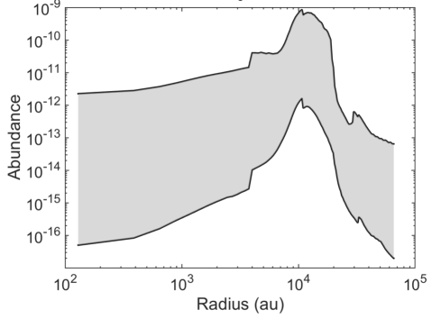
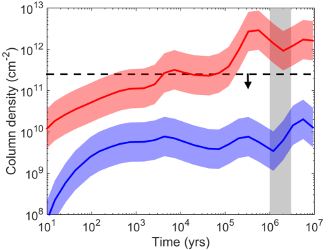
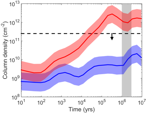
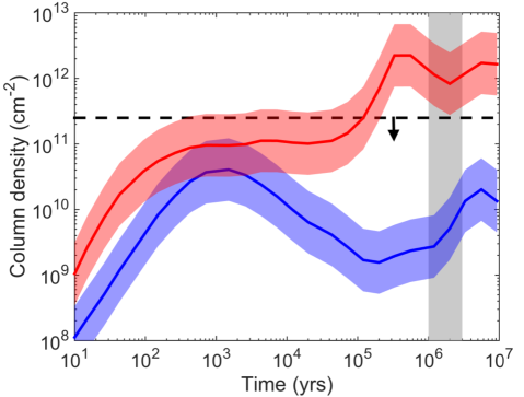
Figure 7: Top panel: Radial distribution of CH₃SH for an age between 10⁶ et 3 $\times$ 10⁶ years, for models 1–6 (see Table 5). Upper to lower panel: Variation of the modelled column density as a function of time and the comparison with the observed upper limit on the column density (dashed black horizontal line). The blue lines correspond to model 1, 2, 3 (sulphur depletion: S/H=$8~{}10^{-8}$) and the red ones correspond to model 4, 5, 6 (sulphur non depletion: S/H=$1.5~{}10^{-5}$) as shown in Table 5. A variation by a factor of three of modelled column densities is shown in corresponding coloured areas. The gray vertical area highlights an age between [1–3] $\times$ 10⁶ years (see text).

To summarize, we used the ten detected species (CCS, C₃S, SO₂, CS, OCS, H₂CS, HSCN, NS, NS⁺, HCS⁺) and some of their isotopologues, as well as the lower limits on both SO and H₂S, and the upper limit on CH₃SH, to constrain the sulphur depletion in the L1544 pre-stellar core. The true degree of depletion of sulphur is difficult to constrain, but the results from our chemical modelling are consistent with a core where the initial sulphur elemental abundance is depleted with respect to the cosmic value (depletion $\sim$ 190). This is in contradiction with what was found by Vidal et al. (2017) towards the starless core TMC-1 (CP). However, the method used by Vidal et al. (2017) is very different from ours, since we are taking into account the density profile of the L1544 pre-stellar core. Their results might prove much different in case the density profile of TMC-1 (CP) is not flat. It is also difficult to compare our results with the study of the Barnard B1b globule which represents an advanced stage compared to L1544 and shows many structures in one beam. Higher spatial resolution is needed for Barnard B1b, to determine the possible influence of the B1b-S outflow on the sulphur chemistry.

6 Conclusions

We presented all the sulphur-bearing species that have been detected in a proto-typical pre-stellar core, L1544, using a spectral survey performed at the IRAM-30m. We computed the column densities for each species and compared them with the results from a chemical modelling taking into account the recent release from a sulphur chemical network. All species from this network are emitted in the external layer of the pre-stellar core, at about 10000 au, and the observations are best reproduced using an initial gas-phase sulphur abundance of 8 $\times$ 10^-8, 0.5$\%$ the cosmic value of 1.5 $\times$ 10^-5. Sulphur is likely depleted in the cold and dense phases of the interstellar medium, although there is no strong evidence of sulphur in the observations of the ice mantles so far.

Appendix A Observations

Table 6: Properties of the observed transitions. The spectroscopic parameters are from CDMS (Müller et al., 2005) except for NS⁺ (Cernicharo et al., 2018), and CC³⁴S (JPL). The rms has been computed over a range of 15 km s^-1 with a spectral resolution of 50 kHz.

Species	QN	Frequency (GHz)	$\rm E_{up}(K)$	$\rm A_{ij}~{}(s^{-1})$	rms (mK)	$\rm T_{mb}~{}(mK)$	$\rm W~{}(mK~{}km~{}s^{-1})$	$\rm FWHM~{}(km~{}s^{-1})$	$\rm V_{LSR}$
CS	20 – 10	$97.98095$	$7.05$	$1.68~{}10^{-5}$	$3.3$	$1226.5\pm 0.1$	$832.1\pm 91.1$	$0.64\pm 0.07$	$7.19\pm 0.03$
13CS	20 – 10	$92.49431$	$6.66$	$1.41~{}10^{-5}$	$2.3$	$120.8\pm 4.1$	$56.3\pm 3.2$	$0.44\pm 0.01$	$7.28\pm 0.01$
C34S	20 – 10	$96.41295$	$6.94$	$1.60~{}10^{-5}$	$3.2$	$391.4\pm 4.2$	$156.6\pm 21.3$	$0.40\pm 0.05$	$7.16\pm 0.01$
CCS	67 – 56	$81.50517$	$15.39$	2.43 $10^{-5}$	$6.8$	$725.9\pm 12.7$	$346.3\pm 13.8$	$0.45\pm 0.01$	$7.07\pm 0.01$
	65 – 54	$72.32379$	$19.21$	1.60 $10^{-5}$	$8.5$	$261.7\pm 12.7$	$116.5\pm 11.2$	$0.42\pm 0.02$	$7.15\pm 0.01$
	78 – 67	$93.87011$	$19.89$	$3.74$ $10^{-5}$	$3.2$	$472.3\pm 21.9$	$225.3\pm 21.7$	$0.45\pm 0.02$	$7.23\pm 0.01$
	66 – 55	$77.73171$	$21.76$	2.03 $10^{-5}$	$5.2$	$179.2\pm 8.4$	$85.5\pm 7.8$	$0.45\pm 0.02$	$7.15\pm 0.01$
	76 – 65	$86.18139$	$23.35$	2.78 $10^{-5}$	$3.4$	$137.2\pm 4.9$	$62.5\pm 5.1$	$0.43\pm 0.02$	$7.13\pm 0.01$
	89 – 78	$106.34773$	$25.00$	$5.48$ $10^{-5}$	$4.2$	$219.6\pm 7.6$	$109.4\pm 8.4$	$0.47\pm 0.02$	$7.16\pm 0.01$
	77 – 66	$90.68638$	$26.12$	$3.29$ $10^{-5}$	$3.5$	$113.7\pm 6.7$	$54.2\pm 6.8$	$0.45\pm 0.03$	$7.18\pm 0.01$
	87 – 76	$99.86652$	$28.14$	$4.40$ $10^{-5}$	$2.6$	$75.5\pm 4.5$	$40.8\pm 4.8$	$0.51\pm 0.03$	$7.22\pm 0.02$
	88 – 77	$103.64076$	$31.09$	$4.90$ $10^{-5}$	$5.2$	$53.5\pm 6.2$	$25.0\pm 5.7$	$0.44\pm 0.05$	$7.15\pm 0.02$
CC34S	67 – 56	$79.827457$	$15.08$	$2.31$ $10^{-5}$	$4.8$	$38.3\pm 4.4$	$18.7\pm 4.6$	$0.46\pm 0.06$	$7.30\pm 0.03$
	78 – 67	$91.9135291$	$19.49$	$3.56$ $10^{-5}$	$2.0$	$21.5\pm 1.9$	$9.1\pm 1.7$	$0.40\pm 0.04$	$7.24\pm 0.02$
C3S	13 – 12	75.14793	25.25	3.26 10-5	$3.0$	$108.7\pm 4.7$	$49.5\pm 4.4$	$0.43\pm 0.02$	$7.26\pm 0.01$
	14 – 13	80.92818	29.13	4.09 10-5	$5.4$	$72.5\pm 7.8$	$32.3\pm 7.3$	$0.42\pm 0.05$	$7.17\pm 0.02$
	15 – 14	86.70838	33.29	5.04 10-5	$2.5$	$76.5\pm 3.1$	$48.7\pm 4.4$	$0.60\pm 0.03$	$7.43\pm 0.01$
	16 – 15	92.48849	37.73	6.13 10-5	$2.5$	$23.7\pm 2.0$	$10.8\pm 1.9$	$0.43\pm 0.04$	$7.22\pm 0.02$
H2S	11,0 – 10,1	168.76276	27.88	$2.68$ $10^{-5}$	9.1		$179.8\pm 3.3$
H2CS	31,3 – 21,2	$101.4778$	$22.91$	$1.26$ $10^{-5}$	$4.0$	$558.4\pm 11.7$	$260.4\pm 11.4$	$0.44\pm 0.01$	$7.19\pm 0.01$
	30,3 – 20,2	$103.0405$	$9.89$	$1.48$ $10^{-5}$	$5.6$	$536.9\pm 16.5$	$256.1\pm 19.3$	$0.45\pm 0.02$	$7.20\pm 0.01$
	31,2 – 21,1	$104.6170$	$23.21$	$1.38$ $10^{-5}$	$4.1$	$514.3\pm 12.0$	$239.9\pm 11.0$	$0.44\pm 0.01$	$7.22\pm 0.01$
H2C34S	31,3 – 21,2	99.77412	22.76	1.20 10-5	3.1	24.8 $\pm$ 1.6	$12.6\pm 1.6$	0.48 $\pm$ 0.03	7.31 $\pm$ 0.01
	30,3- - 20,2	101.2843	9.72	1.41 10-5	3.2	26.5 $\pm$ 3.0	$12.1\pm 3.3$	0.43 $\pm$ 0.07	7.20 $\pm$ 0.03
	31,2 – 21,1	102.8074	23.05	1.31 10-5	4.9	26.1 $\pm$ 3.1	$11.6\pm 2.8$	0.42 $\pm$ 0.05	7.20 $\pm$ 0.02
HDCS	31,3 – 21,2	$91.17107$	$17.73$	$9.12$ $10^{-6}$	$3.0$	$47.2\pm 2.3$	$22.5\pm 2.1$	$0.45\pm 0.02$	$7.16\pm 0.01$
	30,3 – 20,2	$92.98160$	$8.93$	$1.09$ $10^{-5}$	$2.7$	$157.8\pm 7.7$	$76.9\pm 7.1$	$0.46\pm 0.02$	$7.23\pm 0.01$
	31,2 – 21,1	$94.82849$	$18.09$	$1.03$ $10^{-5}$	$3.0$	$38.5\pm 4.6$	$18.4\pm 3.0$	$0.45\pm 0.02$	$7.16\pm 0.01$
D2CS	$313--212$	$83.07776$	$14.32$	$7.00$ $10^{-6}$	$3.9$	$19.2\pm 2.6$	$11.6\pm 3.4$	$0.57\pm 0.09$	$7.30\pm 0.04$
	$303--202$	$85.15392$	$8.18$	$8.48$ $10^{-6}$	$4.0$	$85.2\pm 4.7$	$44.3\pm 4.3$	$0.49\pm 0.02$	$7.20\pm 0.01$
	$312--211$	$87.3027$	$14.72$	$8.12$ $10^{-6}$	$6.3$	$19.3\pm 2.0$	$8.6\pm 3.6$	$0.42\pm 0.13$	$7.17\pm 0.05$
	$414--313$	$110.7561$	$19.63$	$1.81$ $10^{-5}$	$5.0$	$27.1\pm 3.1$	$13.2\pm 2.9$	$0.46\pm 0.05$	$7.29\pm 0.02$
HSCN	80,8 – 70,7	$91.75064$	$19.82$	$4.69$ $10^{-5}$	$2.1$	$14.3\pm 1.5$	$5.9\pm 1.0$	$0.39\pm 0.03$	$7.21\pm 0.01$
OCS	$6--5$	$72.97678$	$12.26$	$1.07$ $10^{-6}$	$3.5$	$106.3\pm 6.8$	$40.6\pm 3.7$	$0.36\pm 0.01$	$7.18\pm 0.01$
	$7--6$	$85.13910$	$16.34$	$1.71$ $10^{-6}$	$4.1$	$87.4\pm 7.2$	$35.2\pm 3.8$	$0.38\pm 0.01$	$7.19\pm 0.01$
	$8--7$	$97.30121$	$21.01$	$2.58$ $10^{-6}$	$4.7$	$70.5\pm 5.4$	$27.7\pm 2.9$	$0.37\pm 0.01$	$7.19\pm 0.01$
	$9--8$	$109.4631$	$26.27$	$3.70$ $10^{-6}$	$4.6$	$49.4\pm 6.4$	$17.8\pm 4.4$	$0.34\pm 0.04$	$7.15\pm 0.02$
SO	$22--11$	$86.09395$	$19.31$	$5.25$ $10^{-6}$	$3.2$	$223.7\pm 5.9$	$100.0\pm 5.0$	$0.42\pm 0.01$	$7.162\pm 0.002$
	$23--12$	$99.29987$	$9.23$	$1.13$ $10^{-5}$	$2.8$	$1422.5\pm 40.6$	$678.5\pm 34.4$	$0.45\pm 0.01$	$7.10\pm 0.01$
	$32--21$	$109.2522$	$21.05$	$1.08~{}10^{-5}$	$3.9$	$176.1\pm 5.2$	$72.8\pm 4.0$	$0.39\pm 0.01$	$7.31\pm 0.01$
S18O	$23--12$	$93.26727$	$8.72$	$9.34~{}10^{-6}$	$2.6$	$21.3\pm 2.1$	$55.9\pm 2.5$	$0.36\pm 0.02$	$6.85\pm 0.01$
34SO	$23--12$	$97.71539$	$9.09$	$1.09~{}10^{-5}$	$4.4$	$85.2\pm 3.9$	$223.3\pm 4.1$	$0.36\pm 0.01$	$6.93\pm 0.01$
SO2	31,3 – 20,2	104.0294	$7.74$	$1.01$ $10^{-5}$	$6.9$	$153.7\pm 8.7$	$60.3\pm 6.7$	$0.37\pm 0.02$	$7.20\pm 0.01$
	60,6 – 51,5	72.75824	19.16	2.77 10-6	4.5	110.23 $\pm$ 0.01	$34.6\pm 3.9$	0.34 $\pm$ 0.02	7.20 $\pm$ 0.01
NS	2$\pi_{1/2}$ 5/21,7/2 – 3/2-1,5/2	$115.15393$	$8.84$	$2.33$ $10^{-5}$	$15.1$	$158.7\pm 8.9$	$74.0\pm 7.5$	$0.44\pm 0.02$	$7.35\pm 0.01$
	2$\pi_{1/2}$ 5/21,5/2 – 3/2-1,3/2	$115.15681$	$8.84$	$1.96$ $10^{-5}$	$15.0$	$108.5\pm 18.2$	$41.4\pm 17.3$	$0.36\pm 0.09$	$7.38\pm 0.04$
	2$\pi_{1/2}$ 5/21,3/2 – 3/2-1,1/2	$115.16298$	$8.84$	$1.75$ $10^{-5}$	$14.6$	$61.1\pm 9.0$	$34.3\pm 9.6$	$0.53\pm 0.07$	$7.54\pm 0.03$
	2$\pi_{1/2}$ 5/2-1,7/2 – 3/21,5/2	$115.55625$	$8.90$	$2.35$ $10^{-5}$	$17.8$	$129.7\pm 7.4$	$49.5\pm 5.6$	$0.36\pm 0.02$	$6.95\pm 0.01$
NS+	2 – 1	100.19855	7.22	$2.21~{}10^{-5}$	3.4	13.7 $\pm$ 1.3	8.6 $\pm$ 1.8	0.59 $\pm$ 0.07	6.95 $\pm$ 0.03
HCS+	2 – 1	$85.34789$	$6.14$	$1.11$ $10^{-5}$	$3.8$	$246.8\pm 6.1$	$112.5\pm 5.4$	$0.43\pm 0.01$	$7.33\pm 0.01$
HC34S+	2 – 1	$83.96563$	$6.04$	$1.06$ $10^{-5}$	$4.1$	$22.4\pm 4.0$	$8.6\pm 3.2$	$0.36\pm 0.07$	$7.35\pm 0.03$

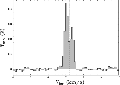
Figure 11: ortho-H₂S transition at 168.8 GHz (in $\rm T_{mb}$).

Appendix B The puzzling behaviour of the H₂S line profile

From the radial variation of the H₂S abundance predicted by the nautilus chemical modelling, we now are able to tentatively reproduce its puzzling line profile. We extracted the H₂S abundance as a function of radius for 20 ages between 10² and 10⁷ years and used the gass code (Quénard et al., 2017a) alongside the structure of L1544 to generate a 3D model of the source. We then use lime (Brinch & Hogerheijde, 2010), which is a 3D non-LTE ALI (Accelerated Lambda Iteration) continuum and gas line radiative transfer treatment, to produce the line intensity data cube. Since the H₂S collision coefficients are not available, we instead used the ortho-H₂O collision coefficients with para–H₂ from Dubernet et al. (2006) as a first approximation. The lime data cubes have been post-processed by gass to extract the H₂S spectra and compare them to the observation. We found that no model extracted from nautilus can satisfactorily reproduce the absorption feature seen at the V_LSR of L1544 in Fig. 11. Fig. 20 shows the result from the nautilus chemical modelling for an age between 10⁶ and 3 10⁶ years, for models 1-3 (see Table 5).

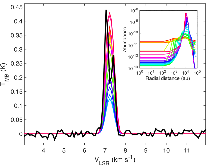
Figure 20: Variation of the calculated H₂S 1_1,0 – 1_0,1 profile (in color) using the variation of the H₂S abundance from the nautilus modelling, for an age between 10⁶ and 3 10⁶ years, for models 1–3 (see Table 5). The profiles are compared with the observed transition in black.

Considering the similarities between the H₂O and H₂S molecules, we then tried the same water abundance profile as the one found by Quénard et al. (2016). We multiplied this profile by factors ranging [1–10] to take into account the different abundances of these two species. The resulting line shapes are shown in Fig. 21 with a small inset presenting some of the abundance profiles used. As one can notice, the absorption can be reproduced for models with a similar (or close by a factor of $\sim$3) abundance profile than the one derived for water by Quénard et al. (2016). However the line is too intense by a scaling factor of $\sim$2.5 (see e.g. red and orange line profiles of Fig. 21). This could be caused by the collision coefficient that we have used as an approximation, which might not be appropriate for H₂S.
To consolidate our findings, we have also considered different ad-hoc abundance profiles to try to better reproduce the observed absorption feature. We have tried $\sim$100 different abundance profile shapes (such as constant abundance as a function of the radius, slope of abundances between two radii, step-function of abundances starting at different radii) but none of them produces a better fit to the observation. Dilution has not been considered since it contradicts the results from the chemical modelling and the maps performed in this source by Spezzano et al. (2017). We therefore concluded that more accurate collision rates might be needed for H₂S with at least para–H₂ and their use will possibly help to better reproduce the observed line profile and constrain the chemistry.

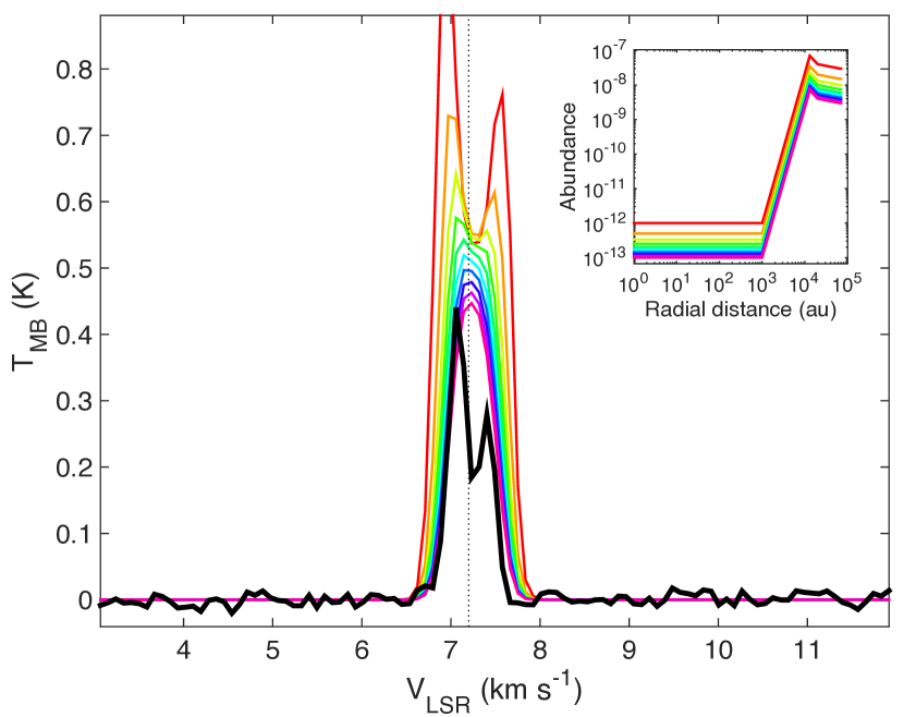
Figure 21: Variation of the calculated H₂S 1_1,0 – 1_0,1 profile (in color) using various ad-hoc abundance profiles (see the inset), compared with the observation (in black).

Appendix C Additional chemical modelling

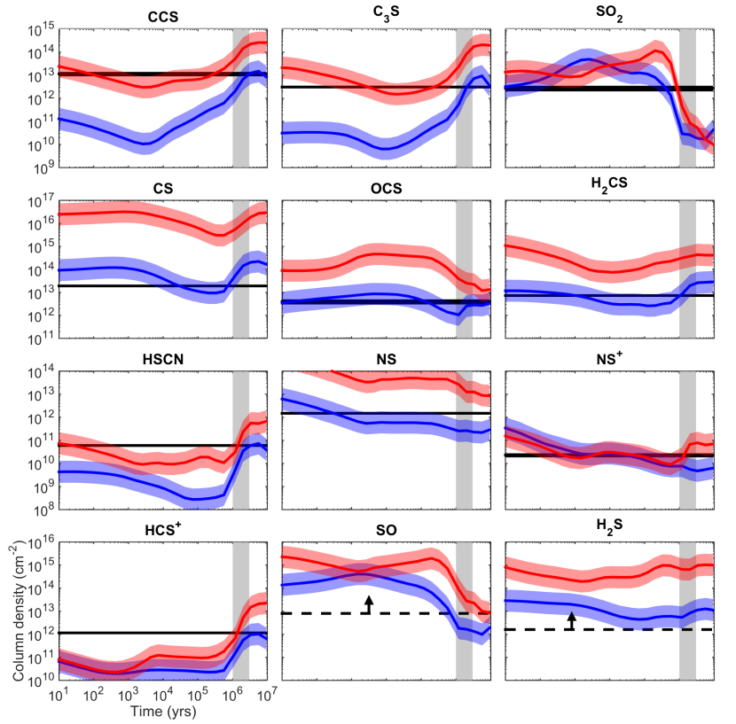
Figure 23: Variation of the modelled column density as a function of time and the comparison with the observed column density (black horizontal line). The blue lines correspond to model 3 (sulphur depletion: S/H=$8~{}10^{-8}$) and the red ones correspond to model 6 (sulphur non depletion: S/H=$1.5~{}10^{-5}$) as shown in Table 5. The thickness of the black line corresponds to the error bar of the observed column densities. A variation by a factor of three of modelled column densities is shown in corresponding coloured areas. The dashed black horizontal line for SO and H₂S correspond to the lower limit on the computation of the total column density. The gray vertical area highlights an age between [1–3] $\times$ 10⁶ years (see text).

References

- Agúndez & Wakelam (2013) Agúndez M., Wakelam V., 2013, Chemical Reviews, 113, 8710
- Agúndez et al. (2018) Agúndez M., Marcelino N., Cernicharo J., Tafalla M., 2018, Astronomy and Astrophysics, 611, L1
- Aikawa et al. (2003) Aikawa Y., Ohashi N., Herbst E., 2003, The Astrophysical Journal, 593, 906
- Anderson et al. (2013) Anderson D. E., Bergin E. A., Maret S., Wakelam V., 2013, The Astrophysical Journal, 779, 141
- Asplund et al. (2009) Asplund M., Grevesse N., Sauval A. J., Scott P., 2009, Annual Review of Astronomy and Astrophysics, 47, 481
- Bachiller & Pérez Gutiérrez (1997) Bachiller R., Pérez Gutiérrez M., 1997, The Astrophysical Journal Letters, 487, 93
- Balucani et al. (2015) Balucani N., Ceccarelli C., Taquet V., 2015, Monthly Notices of the Royal Astronomical Society, 449, 16
- Bizzocchi et al. (2014) Bizzocchi L., Caselli P., Spezzano S., Leonardo E., 2014, Astronomy and Astrophysics, 569, A27
- Boogert et al. (1997) Boogert A. C. A., Schutte W. A., Helmich F. P., Tielens A. G. G. M., Wooden D. H., 1997, Astronomy and Astrophysics, 317, 929
- Brinch & Hogerheijde (2010) Brinch C., Hogerheijde M. R., 2010, Astronomy & Astrophysics, 523, A25
- Calmonte et al. (2016) Calmonte U., et al., 2016, Monthly Notices of the Royal Astronomical Society, 462, 253
- Caselli et al. (1999) Caselli P., Walmsley C. M., Tafalla M., Dore L., Myers P. C., 1999, The Astrophysical Journal Letters, 523, L165
- Caselli et al. (2003) Caselli P., van der Tak F. F. S., Ceccarelli C., Bacmann A., 2003, Astronomy and Astrophysics, 403, L37
- Caselli et al. (2012) Caselli P., et al., 2012, The Astrophysical Journal Letters, 759, L37
- Ceccarelli et al. (2003) Ceccarelli C., Maret S., Tielens A. G. G. M., Castets A., Caux E., 2003, Astronomy and Astrophysics, 410, 587
- Ceccarelli et al. (2014) Ceccarelli C., Caselli P., Bockelée-Morvan D., Mousis O., Pizzarello S., Robert F., Semenov D., 2014, Protostars and Planets VI, pp 859–882
- Cernicharo et al. (2011) Cernicharo J., et al., 2011, Astronomy and Astrophysics, 531, 103
- Cernicharo et al. (2018) Cernicharo J., et al., 2018, Accepted for publication in ApJ Letters
- Chin et al. (1996) Chin Y.-N., Henkel C., Whiteoak J. B., Langer N., Churchwell E. B., 1996, Astronomy and Astrophysics, 305, 960
- Crapsi et al. (2005) Crapsi A., Caselli P., Walmsley C. M., Myers P. C., Tafalla M., Lee C. W., Bourke T. L., 2005, The Astrophysical Journal, 619, 379
- Druard & Wakelam (2012) Druard C., Wakelam V., 2012, Monthly Notices of the Royal Astronomical Society, 426, 354
- Dubernet et al. (2006) Dubernet M.-L., et al., 2006, Astronomy and Astrophysics, 460, 323
- Esplugues et al. (2014) Esplugues G. B., Viti S., Goicoechea J. R., Cernicharo J., 2014, Astronomy and Astrophysics, 567, 95
- Ferrante et al. (2008) Ferrante R. F., Moore M. H., Spiliotis M. M., Hudson R. L., 2008, the Astrophysical Journal, 684, 1210
- Fuente et al. (2016) Fuente A., et al., 2016, A&A, 593, A94
- Garozzo et al. (2010) Garozzo M., Fulvio D., Kanuchova Z., Palumbo M. E., Strazzulla G., 2010, Astronomy and Astrophysics, 509, 67
- Geballe et al. (1985) Geballe T. R., Baas F., Greenberg J. M., Schutte W., 1985, Astronomy and Astrophysics, 146, 6
- Goicoechea et al. (2006) Goicoechea J. R., Pety J., Gerin M., Teyssier D., Roueff E., Hily-Blant P., Baek S., 2006, Astronomy and Astrophysics, 456, 565
- Green & Chapman (1978) Green S., Chapman S., 1978, The Astrophysical Journal Supplement Series, 37, 169
- Hirota et al. (1998) Hirota T., Yamamoto S., Mikami H., Ohishi M., 1998, The Astrophysical Journal, 503, 717
- Howk et al. (2006) Howk J. C., Sembach K. R., Savage B. D., 2006, The Astrophysical Journal, 637, 333
- Jenkins (2009) Jenkins E. B., 2009, The Astrophysical Journal, 700, 1299
- Jiménez-Escobar & Muñoz Caro (2011) Jiménez-Escobar A., Muñoz Caro G. M., 2011, Astronomy and Astrophysics, 536, 91
- Keto et al. (2014) Keto E., Rawlings J., Caselli P., 2014, Monthly Notices of the Royal Astronomical Society, 440, 2616
- Lefloch et al. (2018) Lefloch B., et al., 2018, accepted for publication in MNRAS
- Lique et al. (2007) Lique F., Senent M.-L., Spielfiedel A., Feautrier N., 2007, Journal of Chemical Physics, 126, 164312
- Manfroid et al. (2009) Manfroid J., et al., 2009, Astronomy and Astrophysics, 503, 613
- Marcelino et al. (2005) Marcelino N., Cernicharo J., Roueff E., Gerin M., Mauersberger R., 2005, the Astrophysical Journal, 620, 308
- Milam et al. (2005) Milam S. N., Savage C., Brewster M. A., Ziurys L. M., Wyckoff S., 2005, The Astrophysical Journal, 634, 1126
- Millar & Herbst (1990) Millar T. J., Herbst E., 1990, The Astrophysical Journal, 231, 466
- Müller et al. (2005) Müller H. S. P., Schlöder F., Stutzki J., Winnewisser G., 2005, Journal of Molecular Structure, 742, 215
- Palumbo et al. (1995) Palumbo M. E., Tielens A. G. G. M., Tokunaga A. T., 1995, the Astrophysical Journal, 449, 674
- Palumbo et al. (1997) Palumbo M. E., Geballe T. R., Tielens A. G. G. M., 1997, the Astrophysical Journal, 479, 839
- Pickett et al. (1998) Pickett H. M., Poynter R. L., Cohen E. A., Delitsky M. L., Pearson J. C., Müller H. S. P., 1998, Journal of Quantitative Spectroscopy and Radiative Transfer, 60, 883
- Quénard et al. (2016) Quénard D., Taquet V., Vastel C., Caselli P., Ceccarelli C., 2016, Astronomy and Astrophysics, 585, A36
- Quénard et al. (2017a) Quénard D., Bottinelli S., Caux E., 2017a, Monthly Notices of the Royal Astronomical Society, 468, 685
- Quénard et al. (2017b) Quénard D., Vastel C., Ceccarelli C., Hily-Blant P., Lefloch B., Bachiller R., 2017b, MNRAS, 470, 3194
- Roberts et al. (2003) Roberts H., Herbst E., Millar T. J., 2003, The Astrophysical Journal Letters, 591, L41
- Roberts et al. (2007) Roberts J. F., Rawlings J. M. C., Viti S., Williams D. A., 2007, Monthly Notices of the Royal Astronomical Society, 382, 733
- Ruaud et al. (2016) Ruaud M., Wakelam V., Hersant F., 2016, Monthly Notices of the Royal Astronomical Society, 459, 3756
- Ruffle et al. (1999) Ruffle D. P., Hartquist T. W., Caselli P., Williams D. A., 1999, Monthly Notices of the Royal Astronomical Society, 306, 691
- Scappini et al. (2003) Scappini F., Cecchi-Pestellini C., Smith H., Klemperer W., Dalgarno A., 2003, Monthly Notices of the Royal Astronomical Society, 341, 657
- Smith (1991) Smith R. G., 1991, Monthly Notices of the Royal Astronomical Society, 249, 172
- Spezzano et al. (2017) Spezzano S., Caselli P., Bizzocchi L., Giuliano B. M., Lattanzi V., 2017, Astronomy and Astrophysics, 606, 82
- Tafalla et al. (2002) Tafalla M., Myers P. C., Caselli P., Walmsley C. M., Comito C., 2002, Systematic Molecular Differentiation in Starless Cores, 569, 815
- Tafalla et al. (2006) Tafalla M., Santiago-García J., Myers P. C., Caselli P., Walmsley C. M., Crapsi A., 2006, The Astrophysical Journal, 455, 577
- Tieftrunk et al. (1994) Tieftrunk A., Pineau des Forets G., Schilke P., Walmsley C. M., 1994, Astronomy and Astrophysics, 289, 579
- Tielens (1983) Tielens A. G. G. M., 1983, Astronomy and Astrophysics, pp 177–184
- Vastel et al. (2004) Vastel C., Phillips T. G., Yoshida H., 2004, The Astrophysical Journal Letters, 606, 127
- Vastel et al. (2014) Vastel C., Ceccarelli C., Lefloch B., Bachiller R., 2014, The Astrophysical Journal Letters, 795, L2
- Vastel et al. (2015) Vastel C., Bottinelli S., Caux E., Glorian J.-M., Boiziot M., 2015, in SF2A-2015: Proceedings of the Annual meeting of the French Society of Astronomy and Astrophysics. Eds.: F. Martins, S. Boissier, V. Buat, L. Cambrésy, P. Petit, pp.313-316. pp 313–316, http://sf2a.eu/proceedings/2015/2015sf2a.conf..0313V.pdf
- Vastel et al. (2016) Vastel C., Ceccarelli C., Lefloch B., Bachiller R., 2016, Astronomy and Astrophysics, 591, L2
- Vastel et al. (2018) Vastel C., Kawaguchi K., Quénard D., Ohishi M., Lefloch B., Bachiller R., Müller H. S. P., 2018, Monthly Notices of the Royal Astronomical Society: Letters
- Vasyunin et al. (2017) Vasyunin A. I., Caselli P., Dulieu F., Jiménez-Serra I., 2017, The Astrophysical Journal, 842, 33
- Vidal et al. (2017) Vidal T. H. G., Loison J.-C., Jaziri A. Y., Ruaud M., Gratier P., Wakelam V., 2017, Monthly Notices of the Royal Astronomical Society, 469, 435
- Wakelam et al. (2004) Wakelam V., Caselli P., Ceccarelli C., Herbst E., Castets A., 2004, Astronomy and Astrophysics, 422, 159
- Wakelam et al. (2006) Wakelam V., Herbst E., Selsis F., 2006, Astronomy and Astrophysics, 451, 551
- Wilson (1999) Wilson T. L., 1999, Reports on Progress in Physics, 62
- Zasowski et al. (2009) Zasowski G., Kemper F., Watson D. M., Furlan E., Bohac C. J., Hull C., Green J. D., 2009, Astrophysical Journal, 694, 459