Optimal balancing of time-dependent confounders for marginal structural models

Abstract

Marginal structural models (MSMs) estimate the causal effect of a time-varying treatment in the presence of time-dependent confounding via weighted regression. The standard approach of using inverse probability of treatment weighting (IPTW) can lead to high-variance estimates due to extreme weights and be sensitive to model misspecification. Various methods have been proposed to partially address this, including truncation and stabilized-IPTW to temper extreme weights and covariate balancing propensity score (CBPS) to address treatment model misspecification. In this paper, we present Kernel Optimal Weighting (KOW), a convex-optimization-based approach that finds weights for fitting the MSM that optimally balance time-dependent confounders while simultaneously penalizing extreme weights, directly addressing the above limitations. We further extend KOW to control for informative censoring. We evaluate the performance of KOW in a simulation study, comparing it with IPTW, stabilized-IPTW, and CBPS. We demonstrate the use of KOW in studying the effect of treatment initiation on time-to-death among people living with human immunodeficiency virus and the effect of negative advertising on elections in the United States.

Keywords: causal inference, optimization, covariate balance, time-dependent treatments, marginal structural models

1 Introduction

Marginal structural models (MSMs) offer a successful way to estimate the causal effect of a time-varying treatment on an outcome of interest from longitudinal data in observational studies (Robins, 2000; Robins et al., 2000). For example, they have been used to estimate the optimal timing of HIV treatment initiation (HIV-Causal Collaboration, 2011), to evaluate the effect of hormone therapy on cardiovascular outcomes (Hernán et al., 2008), and to evaluate the impact of negative advertising on election outcomes (Blackwell, 2013). The increasing popularity of MSMs among applied researchers derives from their ability to control for time-dependent confounders, which are confounders that are affected by previous treatments and affect future ones. In particular, as shown by Robins et al. (2000) and Blackwell (2013), standard methods, such as regression or matching, fail to control for time-dependent confounding, introducing post-treatment bias. In contrast, MSMs consistently estimate the causal effect of a time-varying treatment via inverse probability of treatment weighting (IPTW), which controls for time-dependent confounding by weighting each subject under study by the inverse of their probability of being treated given covariates, i.e., the propensity score (Rosenbaum and Rubin, 1983), mimicking a sequential randomized trial. In other words, IPTW creates a hypothetical pseudo-population where time-dependent confounders are balanced over time.

Despite their wide range of applications, the usage of these methods in observational studies may be jeopardized by their considerable dependence on positivity. This assumption requires that, at each time period, the probability of being assigned to the treatment, conditional on the history of treatment and confounders, is not 0 or 1 (Robins, 2000). Even if positivity holds theoretically, when propensities are close to 0 or 1, it can be practically violated. Practical positivity violations lead to extreme and unstable weights, which in turn yield very low precision and misleading inferences (Kang and Schafer, 2007; Robins et al., 1995; Scharfstein et al., 1999). In addition, MSMs using IPTW are highly sensitive to misspecification of the treatment assignment model, which can lead to biased estimates (Kang and Schafer, 2007; Lefebvre et al., 2008; Cole and Hernán, 2008).

Various statistical methods have been proposed in an attempt to overcome these challenges. To deal with extreme weights, several authors (Cole and Hernán, 2008; Xiao et al., 2013) have suggested truncation, whereby outlying weights are replaced with less extreme ones. Santacatterina et al. (2019) proposed to use shrinkage instead of truncation as a more direct way to control the bias-variance trade-off. Robins et al. (2000) recommended the use of stabilized-IPTW (sIPTW) where inverse probability weights are normalized by the marginal probability of treatment. To control for misspecification of the treatment assignment model, Imai and Ratkovic (2015) proposed to use the covariate balance propensity score (CBPS), which instead of plugging in a logistic regression estimate of propensity into IPTW finds the logistic model that balances covariates via the generalized method of moments. The method tries to balance the first moment of each covariate even if a logistic model is misspecified (Imai and Ratkovic, 2014).

In this paper, we present and apply Kernel Optimal Weighting (KOW), which provides weights for fitting an MSM that optimally balance time-dependent confounders while controlling for precision. Specifically, by solving a quadratic optimization problem over weights, the proposed method directly minimizes imbalance, defined as the sum of discrepancies between the weighted observed data and the counterfactual of interest over all treatment regimes, while penalizing extreme weights.

This extends the kernel optimal matching method of Kallus (2016) and Kallus et al. (2018) to the longitudinal setting and to dealing with time-dependent confounders, where, similarly to regression and matching, it cannot be applied without introducing post-treatment bias.

The proposed method has several attractive characteristics. First, by optimally balancing time-dependent confounders while penalizing extreme weights, it leads to better accuracy, precision, and total error. In particular, in the simulation study presented in Section 5, we show that the mean squared error (MSE) of the estimated effect of a time-varying treatment obtained by using KOW is lower than that obtained by using IPTW, sIPTW, and CBPS in all considered simulated scenarios. Second, differently from Imai and Ratkovic (2015), where the number of covariate balancing conditions grows exponentially in the number of time periods, KOW only needs to minimize a number of discrepancies that grows linearly in the number of time periods. This feature leads to a lower computational time of KOW compared with CBPS when the total number of time periods increases, as shown in our simulation study in Section 5.2.3 and in our study on the effect of negative advertising on election outcomes in Section 7.2. Third, by optimally balancing covariates, KOW mitigates the effects of possible misspecification of the treatment model. In Section 5, we show that KOW is more robust to model misspecification compared with the other methods. Fourth, KOW can balance non-additive covariate relationships by using kernels, which generalize the structure of conditional expectation functions, and does not restrict weights to follow a fixed logistic (or other parametric) form. In Section 5, we show how KOW compares favorably with the aforementioned methods in all nonlinear scenarios, and in Section 7.2 we use KOW to balance non-additive covariate relationships estimating the effect of negative advertising on election outcomes. Fifth, KOW can be easily generalized to other settings, such as informative censoring. We do just that in Section 6 and, in Section 7.1, we use this extension to study the effect of human immunodeficiency virus (HIV) treatment on time to death among people living with HIV. Finally, KOW can be solved by using off-the-shelf solvers for quadratic optimization.

In the next section, we briefly introduce the literature of MSMs (Section 2). In Section 3 we develop and define KOW. We then discuss some practical guidelines on the use of KOW (Section 4). In Section 5 we report the results of a simulation study aimed at comparing KOW with IPTW, sIPTW, and CBPS. In Section 6, we extend KOW to control for informative censoring. We then present two empirical applications of KOW in medicine and political science (Section 7). We offer some concluding remarks in Section 8.

2 Marginal structural models for longitudinal data

In this section, we briefly review MSMs (Robins, 2000; Robins et al., 2000). Suppose we have a simple random sample with replacement of size $n$ from a population. For each unit $i=1,\ldots,n$ and time period $t=1,\ldots,T$, we denote the binary time-varying treatment variable by $A_{it}$, with $A_{it}=0$ meaning not being treated at time $t$ and $A_{it}=1$ being treated at time $t$, and time-dependent confounders $X_{it}$. We denote by $\overline{A}_{it}=\{A_{i1},\ldots,A_{it}\}$ the treatment history up to time $t$ and by $\overline{X}_{it}=\{X_{i1},\ldots,X_{it}\}$ the history of confounders up to time $t$. $X_{i1}$ represents the time-invariant confounders, i.e., confounders that do not depend on past treatments. We denote by $\overline{a}_{t}$ and $\overline{x}_{t}$ possible realizations of the treatment history $\overline{A}_{it}$ and the confounder history $\overline{X}_{it}$, respectively. We use $\mathbbm{1}[\cdot]$ to denote the indicator so that $\mathbbm{1}\left[\overline{A}_{it}=\overline{a}_{t}\right]$ is the variable that is 1 if $\overline{A}_{it}=\overline{a}_{t}$ and 0 otherwise. To streamline notation, we will refer to $\overline{A}_{iT}$ as $\overline{A}_{i}$, $\overline{a}_{T}$ as $\overline{a}$, $\overline{X}_{iT}$ as $\overline{X}_{i}$, and to $\overline{x}_{T}$ as $\overline{x}$. For each unit $i=1,\ldots,n$, we denote by $Y_{i}$ the outcome variable observed at the end of the study. Using the potential outcome framework (Imbens and Rubin, 2015), we denote by $Y_{i}(\overline{a})$ the potential outcome we would see if we were to apply the treatment regime $\overline{a}\in\mathcal{A}$ to the $i^{\text{th}}$ unit, where $\mathcal{A}=\{0,1\}^{T}$ is the space of treatment regimes. Throughout, we drop the subscripts $i$ on these variables to refer to a generic unit.

We impose the assumptions of consistency, non-interference, positivity and sequential ignorability (Imbens and Rubin, 2015; Hernán and Robins, 2010). Consistency and non-interference (also known as SUTVA; Rubin, 1980) can be encapsulated in that the potential outcomes are well-defined and the observed outcome corresponds to the potential outcome of the treatment regime applied to that unit, i.e., $Y=Y(\overline{A})$. As previously introduced, positivity states that, for each time $t=1,\ldots,T$, the probability of being treated at time $t$ conditioned on the treatment history up to time $t-1$ and the confounder history up to time $t$, is not 0 or 1, i.e.,

$$0<\mathbb{P}(A_{t}=1\mid\overline{A}_{t-1},\overline{X}_{t})<1\quad\forall\ t\in\{1,\ldots,T\},$$ (1)

Sequential ignorability states that the potential outcome $Y(\overline{a})$ is independent of treatment assignment at time $t$, given the treatment history up to time $t-1$ and the confounder history up to time $t$. Formally, sequential ignorability is defined as

$$Y(\overline{a})\mathchoice{\mathrel{\hbox to0.0pt{$\displaystyle\perp$\hss}\mkern 2.0mu{\displaystyle\perp}}}{\mathrel{\hbox to0.0pt{$\textstyle\perp$\hss}\mkern 2.0mu{\textstyle\perp}}}{\mathrel{\hbox to0.0pt{$\scriptstyle\perp$\hss}\mkern 2.0mu{\scriptstyle\perp}}}{\mathrel{\hbox to0.0pt{$\scriptscriptstyle\perp$\hss}\mkern 2.0mu{\scriptscriptstyle\perp}}}A_{t}\mid\overline{A}_{t-1},\overline{X}_{t}\quad\forall\ t\in\{1,\ldots,T\}.$$ (2)

An MSM is a model for the marginal causal effect of a time-varying treatment regime on the mean of $Y$, that is,

$$\mathbbm{E}\left[Y(\overline{a})\right]=g(\overline{a},\bm{\beta}),$$ (3)

where $g(\overline{a},\bm{\beta})$ is some known function class parametrized by $\bm{\beta}$. For example, a commonly used MSM is based on additive effects with a common coefficient: $g(\overline{a},\bm{\beta})=\beta_{1}+\beta_{2}\sum_{t=1}^{T}a_{t}$, where the parameter $\beta_{2}$ is the causal parameter of interest. Usually, $\bm{\beta}$ is computed by a weighted regression of the outcome on the treatment regime alone using weighted least squares (WLS), i.e., $\min_{\bm{\beta}}\sum_{i=1}^{n}W_{i}(Y_{i}-g(\overline{A}_{i},\bm{\beta}))^{2}$, and Wald confidence intervals are constructed using robust (sandwich) standard errors (Freedman, 2006; Robins, 2000; Hernán et al., 2001). In order to consistently estimate $\bm{\beta}$, the weights $W_{1:n}=(W_{1},\dots,W_{n})$, must account for the non-randomness of the treatment assignment mechanism, i.e., the confounding. Robins (2000) showed that the set of inverse probability weights and stabilized inverse probability weights achieve this objective. These weights are defined as follows,

$$W_{i}^{\text{IPTW}}=w(\overline{A}_{i},\overline{X}_{i}),\quad w(\overline{a},\overline{x}) =\prod_{t=1}^{T}\frac{h_{t}(\overline{a}_{t})}{\mathbb{P}(A_{t}=a_{t}\mid\overline{A}_{t-1}=\overline{a}_{t-1},\overline{X}_{t}=\overline{x}_{t})},$$ (4)

where $h_{t}(\overline{a}_{t})$ is a known function of treatment history. The set of inverse probability weights is obtained by setting $h_{t}(\overline{a}_{t})=1$, while the set of stabilized inverse probability weights is obtained by setting $h_{t}(\overline{a}_{t})=\mathbb{P}(A_{t}=a_{t}\mid\overline{A}_{t-1}=\overline{a}_{t-1})$. To estimate weights of the form of eq. (4), one first estimates the conditional probability models using either parametric methods such as logistic regression or other machine learning methods (Karim et al., 2017; Gruber et al., 2015; Karim and Platt, 2017) and then these estimates are plugged in directly into eq. (4) to derive weights, which are then plugged into the WLS. Stabilized weights seek to attenuate the variability of inverse probability weights by normalizing them by the marginal probability of treatment. Since the additional factor is a function of treatment regime alone, it does not affect the consistency of the WLS if the MSM is well specified. Both sets of weights, however, rely on plugging in an estimate of a probability into the denominator, meaning that when the true probability is even modestly close to 0, any small error in estimating it can translate to very large errors in estimating the weights and to estimated weights that are extremely variable. Furthermore, both sets of weights rely on the correct specification of the conditional probability models used to estimate the weights in eq. (4).

To overcome this issue, Imai and Ratkovic (2015) proposed to estimate weights of the form of eq. (4) that improve balance of confounders by generalizing the covariate balancing propensity score (CBPS) methodology. Instead of plugging in probability estimates based on logistic regression, CBPS uses the generalized method of moments to find the logistic regression model that if plugged in would lead to weights, $W_{i}^{\text{CBPS}}$, that approximately solve a subset of the moment conditions that the true inverse probability weights, eq. (4), satisfy.

Differently than IPTW, sIPTW and CBPS, in the next Section, we characterize imbalance as the discrepancies in observed average outcomes due to confounding, consider their worst case values, and use quadratic optimization to obtain weights that directly optimize the balance of time-invariant and time-dependent confounders over all possible weights while controlling precision.

3 Kernel Optimal Weighting

In this Section we present a convex-optimization-based approach that obtains weights that minimize the imbalance due to time-dependent confounding (i.e., maximize balance thereof) while controlling precision. Toward that end, in Section 3.1, we provide a definition of imbalance. Specifically, we define imbalance as the sum of discrepancies between the weighted observed data and the unobserved counterfactual of interest over all treatment regimes. Since this imbalance depends on unknown functions, in Section 3.2 we consider the worst case imbalance, which guards against all possible realizations of the unknown functions. We also show that the worst case imbalance has the attractive characteristic that the number of discrepancies considered grows linearly in the number of time periods and not exponentially like the number of treatment regimes. We finally show how to minimize this quantity while controlling precision using kernels, reproducing kernel Hilbert space (RKHS) and off-the-shelf solvers for quadratic optimization (Sections 3.3-3.4).

3.1 Defining imbalance

Consider any population weights $W=w(\overline{A},\overline{X})$, where $w(\cdot)$ is a function that depends on the treatment and confounder histories. In this Section, we will show that, under consistency and assumptions (1)–(2), we can decompose the difference between the weighted average outcome among the $\overline{a}$-treated units, $\mathbbm{E}[W\mathbbm{1}[\overline{A}=\overline{a}]Y]$, and the average potential outcome of $\overline{a}$, $\mathbbm{E}[Y(\overline{a})]$, into a sum over time points $t$ of discrepancies involving the values of treatment and confounder histories up to time $t$.

To build intuition we start by explaining this decomposition in the case of two time periods $T=2$. Assuming consistency and assumptions (1)–(2), for each $\overline{a}=(a_{1},a_{2})\in\mathcal{A}$, we can decompose the weighted average outcome among the $\overline{a}$-treated units as follows:

$$\mathbb{E}[W\mathbbm{1}[\overline{A}=\overline{a}]Y] =\mathbb{E}[W\mathbbm{1}[A_{1}=a_{1}]\mathbbm{1}[A_{2}=a_{2}]\mathbb{E}[Y(\overline{a})\mid A_{1},A_{2},X_{1},X_{2}]]$$ (5)

$$=\mathbb{E}[W\mathbbm{1}[A_{1}=a_{1}]\mathbbm{1}[A_{2}=a_{2}]\mathbb{E}[Y(\overline{a})\mid A_{1},X_{1},X_{2}]]$$

$$=\mathbb{E}[W\mathbbm{1}[A_{1}=a_{1}]\mathbb{E}[Y(\overline{a})\mid A_{1},X_{1},X_{2}]]+\delta^{(2)}_{a_{2}}(W,g_{\overline{a}}^{(2)})$$

$$=\mathbb{E}[W\mathbbm{1}[A_{1}=a_{1}]\mathbb{E}[Y(\overline{a})\mid X_{1}]]+\delta^{(2)}_{a_{2}}(W,g_{\overline{a}}^{(2)})$$

$$=\mathbb{E}[Y(\overline{a})]+\delta^{(1)}_{a_{1}}(W,g_{\overline{a}}^{(1)})+\delta^{(2)}_{a_{2}}(W,g_{\overline{a}}^{(2)})$$

$$=\mathbb{E}[Y(\overline{a})]+\sum_{t=1}^{2}\delta^{(t)}_{a_{t}}(W,g_{\overline{a}}^{(t)}),$$

where the first equality follows from iterated expectation, the second from sequential ignorability, the fourth from iterated expectation and sequential ignorability and the third and fifth from the following definitions, which exactly capture the difference between the two sides of the third and fifth equalities,

$$\delta^{(2)}_{a_{2}}(W,h^{(2)}) =\mathbbm{E}\left[W\mathbbm{1}[A_{2}=a_{2}]h^{(2)}(A_{1},X_{1},X_{2})\right]-\mathbbm{E}\left[Wh^{(2)}(A_{1},X_{1},X_{2})\right]$$ (6)

$$g_{\overline{a}}^{(2)}(A_{1},X_{1},X_{2}) =\mathbbm{1}[A_{1}=a_{1}]\mathbbm{E}\left[Y(\overline{a})\mid A_{1},X_{1},X_{2}\right]$$

$$\delta^{(1)}_{a_{1}}(W,h^{(1)}) =\mathbbm{E}\left[W\mathbbm{1}[A_{1}=a_{1}]h^{(1)}(X_{1})\right]-\mathbbm{E}\left[h^{(1)}(X_{1})\right]$$

$$g_{\overline{a}}^{(1)}(X_{1}) =\mathbbm{E}\left[Y(\overline{a})\mid X_{1}\right].$$

Note our use of $h^{(t)}$ as a generic dummy function and $g_{\overline{a}}^{(t)}$ as a specific function that depends on the particular (unknown) distribution of $\overline{X}_{t},\overline{A}_{t-1},Y(\overline{a})$.

This gives a definition of discrepancy, $\delta^{(t)}_{a_{t}}(W,h^{(t)})$, where the subscript $a_{t}\in\{0,1\}$ refers to the treatment assigned at time $t$, $W=w(\overline{A},\overline{X})$ is a population weight, and $h^{(t)}$ is a given function of interest of the treatment and confounder history up to $t$, $\overline{A}_{t-1},\overline{X}_{t}$. The function $g_{\overline{a}}^{(t)}$ is one such function. In particular, for every $a_{1}\in\{0,1\}$, the quantity $\delta^{(1)}_{a_{1}}(W,h^{(1)})$ is the discrepancy between the $h^{(1)}$-moments of the baseline confounder distribution in the weighted $a_{1}$-treated population and of the distribution in the whole population. Similarly, for every $a_{2}\in\{0,1\}$, $\delta^{(2)}_{a_{2}}(W,h^{(2)})$ is a discrepancy in the $h^{(2)}$-moment of treatment and confounder histories at the start of time step $2$. What we have shown above is how these discrepancies directly relate to the difference between weighted averages of observed outcomes and true averages of unknown counterfactuals of interest. Specifically, we have shown that when we measure these discrepancies with respect to the specific function $g_{\overline{a}}^{(t)}$, then their sum gives that difference.

We can extend this decomposition to general horizons $T\geq 1$. Let us define the same discrepancies for any time $t\geq 3$ as

$$\delta^{(t)}_{a_{t}}(W,h^{(t)}) =\mathbbm{E}\left[W\mathbbm{1}[A_{t}=a_{t}]h^{(t)}(\overline{A}_{t-1},\overline{X}_{t})\right]-\mathbbm{E}\left[Wh^{(t)}(\overline{A}_{t-1},\overline{X}_{t})\right],$$

$$g_{\overline{a}}^{(t)}(\overline{A}_{t-1},\overline{X}_{t}) =\mathbbm{1}[\overline{A}_{t-1}=\overline{a}_{t-1}]\mathbbm{E}\left[Y(\overline{a})\mid\overline{A}_{t-1},\overline{X}_{t}\right].$$

The following result gives the general decomposition of the difference between weighted average of observed outcomes and true average of counterfactuals as the sum of $T$ discrepancies, one for every time step:

Theorem 1.

Under assumptions (1)–(2), for each $\overline{a}\in\mathcal{A}=\{0,1\}^{T}$,

$$\mathbbm{E}\left[W\mathbbm{1}[\overline{A}=\overline{a}]Y\right]-\mathbbm{E}\left[Y(\overline{a})\right]=\sum_{t=1}^{T}\delta^{(t)}_{a_{t}}(W,g_{\overline{a}}^{(t)}).$$

Based on the results of Theorem 1, it is clear that if we want the difference between average counterfactual outcomes and average weighted factual outcomes to be small for all treatment regimes $\overline{a}$ then we should seek weights $W$ that make

$$\overline{\delta}_{\overline{a}}(W,\overline{g}_{\overline{a}})=\sum_{t=1}^{T}\delta^{(t)}_{a_{t}}(W,g_{\overline{a}}^{(t)})$$

small for all $\overline{a}$, where we write $\overline{h}=(h^{(1)},\dots,h^{(T)})$ for any set of $T$ functions.

The empirical counterparts to $\delta^{(t)}_{a_{t}}(W,h^{(t)})$ are the sample moment discrepancies for a given set of sample weights $W_{1:n}$:

$$\hat{\delta}^{(t)}_{a_{t}}(W_{1:n},h^{(t)}) =\frac{1}{n}\sum_{i=1}^{n}(W_{i}\mathbbm{1}[A_{it}=a_{t}]-W_{i})h^{(t)}(\overline{A}_{i,t-1},\overline{X}_{it}),\quad\forall t\geq 2,$$ (7)

$$\hat{\delta}^{(1)}_{a_{1}}(W_{1:n},h^{(1)}) =\frac{1}{n}\sum_{i=1}^{n}W_{i}\mathbbm{1}[A_{i1}=a_{1}]h^{(1)}(X_{i1})-\frac{1}{n}\sum_{i=1}^{n}h^{(1)}(X_{i1}),$$

$$\hat{\overline{\delta}}_{\overline{a}}(W_{1:n},\overline{h}) =\sum_{t=1}^{T}\hat{\delta}^{(t)}_{a_{t}}(W_{1:n},h^{(t)}).$$

Thus, we will seek samples weights $W_{1:n}$ that make $\hat{\overline{\delta}}_{\overline{a}}(W_{1:n},\overline{g}_{\overline{a}})$ small for all treatment regimes $\overline{a}$. Toward that end, for any set of given functions $(\overline{h}_{\overline{a}})_{\overline{a}\in\mathcal{A}}$, we define imbalance of a set of weights $W_{1:n}$ as the average squared discrepancy over treatment regimes:

$$\text{IMB}(W_{1:n};(\overline{h}_{\overline{a}})_{\overline{a}\in\mathcal{A}}) =\frac{1}{\left|\mathcal{A}\right|}\sum_{\overline{a}\in\mathcal{A}}\hat{\overline{\delta}}^{2}_{\overline{a}}(W_{1:n},\overline{h}_{\overline{a}}).$$ (8)

The particular imbalance of interest is given when we consider $\overline{h}_{\overline{a}}=\overline{g}_{\overline{a}}$. One way to control this imbalance, $\text{IMB}(W_{1:n};(\overline{g}_{\overline{a}})_{\overline{a}\in\mathcal{A}})$, and consequently control the empirical discrepancies of interest, $\hat{\overline{\delta}}_{\overline{a}}(W_{1:n},\overline{g}_{\overline{a}})$, is by using inverse probability weights. If known, these weights make this quantity a sample average of mean-zero variables and thus close to zero for large $n$. However, the difficulties are that (a) even mild practical violations of positivity can lead to large variance of each of these terms and (b) we need to correctly estimate the sequential propensities.

Differently, we will seek to find weights that directly minimize imbalance. There are two main challenges in this task. The first challenge is that the imbalance of interest depends on some unknown functions $\overline{g}_{\overline{a}}$. The second is that the number of treatment regimes grows exponentially in the number of time periods. In the next Section we show how the proposed methodology overcomes these two challenges.

3.2 Worst case imbalance

To overcome the fact that we do not actually know the functions $\overline{g}_{\overline{a}}$ on which imbalance $\text{IMB}(W_{1:n};(\overline{g}_{\overline{a}})_{\overline{a}\in\mathcal{A}})$ depends, we will guard against all possible realizations of the unknown functions. Specifically, since $\hat{\overline{\delta}}_{\overline{a}}(W_{1:n},\overline{g}_{\overline{a}})$ scales linearly with $\overline{g}_{\overline{a}}$, we will consider its magnitude relative to that of $\overline{g}_{\overline{a}}$. We therefore need to define a magnitude. In particular, let us define

$$\|\overline{h}\|=\sqrt{\|h^{(1)}\|^{2}_{(1)}+\cdots+\|h^{(T)}\|^{2}_{(T)}},$$

where $\|\cdot\|^{2}_{(t)}$ are some given extended seminorms on functions from the space of time-dependent confounders and treatment histories up to time $t$ to the space of outcomes. Compared to a norm, an extended seminorm may also assign the values of $0$ and $\infty$ to nonzero elements but must still satisfy triangle inequality and absolute homogeneity. We will discuss specific choices of such seminorms $\|\cdot\|^{2}_{(t)}$ in Section 3.4.

Given these, we can define the worst case discrepancies,

$$\Delta^{(t)}_{a_{t}}(W_{1:n})=\sup_{h^{(t)}}\frac{\hat{\delta}^{(t)}_{a_{t}}(W_{1:n},h^{(t)})}{\|h^{(t)}\|_{(t)}}=\sup_{\|h^{(t)}\|_{(t)}\leq 1}\hat{\delta}^{(t)}_{a_{1}}(W_{1:n},h^{(t)}).$$

Note that $\Delta^{(t)}_{a_{t}}(W_{1:n})$ depends only on the treatment at time $t$, $a_{t}$, and not the whole treatment regime, $\overline{a}$.

Then the worst case imbalance is given by

$$\mathcal{B}^{2}(W_{1:n}) =\sup_{\|\overline{h}_{\overline{a}}\|\leq 1\;\forall\overline{a}\in\mathcal{A}}\text{IMB}(W_{1:n};(\overline{h}_{\overline{a}}^{(t)})_{\overline{a}\in\mathcal{A}})$$ (9)

$$=\sup_{\overline{h}_{\overline{a}},\;\overline{a}\in\mathcal{A}}\frac{1}{\left|\mathcal{A}\right|}\sum_{\overline{a}\in\mathcal{A}}\frac{\hat{\overline{\delta}}^{2}_{\overline{a}}(W_{1:n},\overline{h}_{\overline{a}})}{\|\overline{h}_{\overline{a}}\|^{2}}$$

$$=\frac{1}{2}\sum_{t=1}^{T}(\Delta^{(t)}_{0}(W_{1:n})^{2}+\Delta^{(t)}_{1}(W_{1:n})^{2}).$$

What is important to note is that this shows that the discrepancies of interest are essentially the same regardless of the particular treatment regime trajectory $\overline{a}$. That is, to control the discrepancies for all trajectories $\overline{a}$ for all possible realizations of $\overline{g}_{\overline{a}}$, at any time point $t$, we are only concerned with the discrepancies of histories $\overline{A}_{t-1},\overline{X}_{t}$ for those units treated at time $t$, $A_{t}=1$, and for those not, $A_{t}=0$. So, while the number of treatment regimes grows exponentially in the number of periods, we need only to keep track of and minimize a number of discrepancies growing linearly in the number of periods $T$. By eliminating each of these linearly-many imbalances, any time-dependent confounding would necessarily be removed, as shown by Theorem 1. In Section 5.2.3, we show how this feature also translates to favorable computational time when dealing with many time periods.

3.3 Minimizing imbalance while controlling precision

We can obtain minimal imbalance by minimizing $\mathcal{B}^{2}(W)$. However, to control for extreme weights we propose to regularize the weight variables $W_{1:n}$. We therefore wish to find weights that minimizes $\mathcal{B}^{2}(W_{1:n})$ plus a penalty for deviations from uniform weighting. Formally, we want to solve

$$\underset{W_{1:n}\in\mathcal{W}}{\min}\quad\mathcal{B}^{2}(W_{1:n})+\lambda\|W_{1:n}-e\|_{2}^{2},$$ (10)

where $e$ is the vector of ones and $\mathcal{W}=\{W_{1:n}:W_{i}\geq 0\;\forall i\}$ is the space of nonnegative weights $W_{1:n}$. The squared distance of the weights from uniform weights here serves as a convex surrogate for the variance of the resulting MSM (assuming homoskedasticity or bounded residual variances) and $\lambda$ in eq. (10) can be interpreted as a penalization parameter that controls the trade off between imbalance and precision. When $\lambda$ is equal to zero, the obtained weights provide minimal imbalance. When $\lambda\rightarrow\infty$, the weights become uniformly distributed leading to an ordinary least squares estimator for the MSM.

In the next section, we discuss a specific choice of the norm that specified the worst case discrepancies $\Delta_{a_{t}}^{(t)}(W_{1:n})$, presented in Section 3.2. Specifically, we show that by choosing an RKHS to specify the norm, we can express the optimization problem in eq. (10) as a convex-quadratic function in $W_{1:n}$, which can be easily solved by using off-the-shelf solvers for quadratic optimization.

3.4 RKHS and quadratic optimization to optimally balance time-dependent confounders

An RKHS is a Hilbert space of functions which is associated a kernel (the reproducing kernel). Specifically, any positive semi-definite kernel $\mathcal{K}:\mathcal{Z}\times\mathcal{Z}\to\mathbb{R}$ on a ground space $\mathcal{Z}$ defines a Hilbert space given by (the unique completion of) the span of all functions $\mathcal{K}(z,\cdot)$ for $z\in\mathcal{Z}$, endowed with the inner product $\left<\mathcal{K}(z,\cdot),\mathcal{K}(z^{\prime},\cdot)\right>=\mathcal{K}(z,z^{\prime})$. Kernels are widely used in machine learning to generalize the structure of conditional expectation functions with many applications in statistics (Schölkopf and Smola, 2002; Berlinet and Thomas-Agnan, 2011; Kallus, 2016, 2018). Commonly used kernels are the polynomial, Gaussian, and Matérn kernels (Schölkopf and Smola, 2002).

The following theorem shows that if $\|\cdot\|_{(t)}$, the norm that specified the worst case discrepancies $\Delta_{a_{t}}^{(t)}(W_{1:n})$, is an RKHS norm given by the kernel $\mathcal{K}_{t}$, then we can express it as a convex-quadratic function in $W_{1:n}$.

Theorem 2.

Define the matrix $K_{t}\in\mathbb{R}^{n\times n}$ as

$$K_{tij}=\mathcal{K}_{t}((\overline{A}_{i,t-1},\overline{X}_{it}),(\overline{A}_{j,t-1},\overline{X}_{jt}))$$

and note that it is positive semidefinite by definition. Then, if the norm $\|\cdot\|_{(t)}$ is the RKHS norm given by the kernel $\mathcal{K}_{t}$, the squared worst case discrepancies are

$$\Delta^{(1)}_{a_{1}}(W_{1:n})^{2} =\frac{1}{n^{2}}W_{1:n}^{T}I^{(1)}_{a_{1}}K_{1}I^{(1)}_{a_{1}}W_{1:n}-2e^{T}K_{1}I^{(1)}_{a_{1}}W_{1:n}+e^{T}K_{1}e,$$

$$\Delta^{(t)}_{a_{t}}(W_{1:n})^{2} =\frac{1}{n^{2}}W_{1:n}^{T}(I-I^{(t)}_{a_{t}})K_{t}(I-I^{(t)}_{a_{t}})W_{1:n},$$

where $I$ is the identity matrix and $I^{(t)}_{a_{t}}$ is the diagonal matrix with $\mathbb{I}[A_{it}=a_{t}]$ in its $i^{\text{th}}$ diagonal entry.

Based on Theorem 2, we can now express the worst case imbalance, $\mathcal{B}^{2}(W_{1:n})$, defined in eq. (9), as a convex-quadratic function. Specifically, let $K_{t}^{\circ}={I^{(t)}_{0}K_{t}I^{(t)}_{0}+I^{(t)}_{1}K_{t}I^{(t)}_{1}}$, which is given by setting every entry $i,j$ of $K_{t}$ to 0 whenever $A_{it}\neq A_{jt}$, and $K^{\circ}=\sum_{t=1}^{T}K_{t}^{\circ}$. We then get that

$$\mathcal{B}^{2}(W_{1:n}) =\frac{1}{2}\sum_{t=1}^{T}(\Delta^{(t)}_{0}(W_{1:n})^{2}+\Delta^{(t)}_{1}(W_{1:n})^{2})$$ (11)

$$=\frac{1}{n^{2}}\biggl{(}\frac{1}{2}W_{1:n}^{T}K^{\circ}W_{1:n}-e^{T}K_{1}W_{1:n}+e^{T}K_{1}e\biggr{)}.$$

Finally, to obtain weights that optimally balance covariates to control for time-dependent confounding while controlling precision we solve the quadratic optimization problem,

$$\underset{W_{1:n}\in\mathcal{W}}{\min} \frac{1}{2}W_{1:n}^{T}K_{\lambda}^{\circ}W_{1:n}-e^{T}K_{\lambda}W_{1:n}$$ (12)

where $K_{\lambda}^{\circ}=K^{\circ}+2\lambda I$, $K_{\lambda}=K_{1}+2\lambda I$. We call this proposed methodology and the result of eq. (12), Kernel Optimal Weighting (KOW).

4 Practical guidelines

Solutions to the quadratic optimization problem (12) depend on several factors. First, they depend on the choice of the kernel and its hyperparameters. There are some existing practical guidelines on these choices (Schölkopf and Smola, 2002; Rasmussen and Williams, 2006), on which we rely as explained below. Second, they depend on the penalization parameter $\lambda$. Finally, solutions to eq. (12) depend on the chosen set of lagged covariates to include in each kernel. In this section, we introduce some practical guidelines on how to apply KOW in consideration of these factors.

For each $t$, the unknown function $g_{\overline{a}}^{(t)}(\overline{A}_{t-1},\overline{X}_{t})$ has two distinct inputs: the treatment history and the confounder history. To reflect this structure, we suggest to specify the kernel $\mathcal{K}_{t}$ as a product kernel, i.e.,$\mathcal{K}_{t}((\overline{a}_{t-1},\overline{x}_{t}),(\overline{a}^{\prime}_{t-1},\overline{x}^{\prime}_{t}))=\mathcal{K}_{t}^{(1)}(\overline{a}_{t-1},\overline{a}^{\prime}_{t-1})\mathcal{K}_{t}^{(2)}(\overline{x}_{t},\overline{x}^{\prime}_{t})$ given a treatment history kernel $\mathcal{K}_{t}^{(1)}$ and a confounder history kernel $\mathcal{K}_{t}^{(2)}$. This simplifies the process of specifying the kernels. We further suggest that for the treatment history to use a linear kernel involving $\ell$ lagged treatments, $\mathcal{K}_{t}^{(1)}(\overline{a}_{t-1},\overline{a}^{\prime}_{t-1})=\sum_{s=\max(1,t-\ell)}^{t-1}a_{s}a^{\prime}_{s}$, and for the confounder history to use a polynomial kernel involving the time-invariant confounders and $\ell$ lagged time-dependent confounders, $\mathcal{K}_{t}^{(d)}(\overline{x}_{t},\overline{x}^{\prime}_{t})=(1+\theta x_{1}^{T}x^{\prime}_{1}+\theta\sum_{s=\max(2,t-\ell+1)}^{t}x_{t}^{T}x^{\prime}_{t})^{d}$, where $\theta>0$ and $d\in\mathbb{N}$ are hyperparameters. We discuss the choice of the number of lags and the hyperparameters below. In our simulation study in Section 5, we show that the MSE of the MSM-estimated effect using KOW with a product of linear kernel and a quadratic kernel ($d=2$) outperforms estimates using weights obtained by IPTW, sIPTW and CBPS in all considered simulated scenarios. We again use this choice of kernels in our empirical applications of KOW to real datasets in Section 7. Many other choices of kernel are also possible and may be more appropriate in a particular application, but we suggest the above combination as a generic and successful recipe.

When using kernels, preprocessing the data is an important step. In particular, normalization is employed to avoid unit dependence and covariates with high variance dominating those with smaller ones. Consequently, we suggest, beforehand, to scale the covariates related to the treatment and confounder histories to have mean 0 and variance 1.

To tune the kernels’ hyperparameters and the penalization parameter $\lambda$, we follow Kallus (2016) and use the empirical Bayes approach of marginal likelihood (Rasmussen and Williams, 2006). We postulate a Gaussian process prior $g^{(t)}\sim\mathcal{GP}(c_{t}\mathbf{1},\mathcal{K}_{t}(\theta))$, where $c_{t}\mathbf{1}$ is a constant function and $\mathcal{K}_{t}(\theta_{t})$ is a kernel that depends on some set of hyperparameters $\theta_{t}$. For each $t$, we then maximize the marginal likelihood of seeing the data $Y\sim\mathcal{N}(g^{(t)}(\overline{X}_{t},\overline{A}_{t-1}),\lambda_{t})$ over $\theta_{t},\lambda_{t},c_{t}$ and let $\lambda=\sum_{t=1}^{T}\lambda_{t}$. It would be more correct to consider the marginal likelihood of observing the partial means of outcomes, but we find that this much simpler approach suffices for learning the right representation of the data ($\theta_{t}$) and the right penalization parameter ($\lambda$) and it enables the use of existing packages such as GPML (Rasmussen and Nickisch, 2010). We demonstrate this in the simulations presented in Section 5, and in particular in Figures 3 and 4 we see that this approach leads to a value of the penalization parameter that is near that which minimizes the resulting MSE of the MSM over possible parameters.

Another practical concern is how many lagged covariates to include in each of the kernels $\mathcal{K}_{t}$. When deriving inverse probability weights, it is common to model the denominator in eq. (4) by fitting a pooled logistic model (D’Agostino et al., 1990) including only the time-invariant confounders, $X_{1}$, the time-dependent confounders at time $t$, $X_{t}$, and the one-time lagged treatment history, $A_{t-1}$, rather than the entire histories, i.e., logit $\mathbb{P}(A_{t}=a_{t}\mid\overline{A}_{t-1}=\overline{a}_{t-1},\overline{X}_{t}=\overline{x}_{t})=\alpha_{t}+\beta_{1}A_{t-1}+\beta_{2}X_{1}+\beta_{3}X_{t}$, (Hernán et al., 2001, 2002). This can be understood as a certain Markovian assumption about the data generating process which simplifies the modeling when $T$ is large. The same can be done in the case of KOW, where we may assume that $g_{\overline{a}}^{(t)}$ is only a function of the one-time lagged treatment, the time-dependent counfounders at time $t$, and the time-invariant confounders, i.e., $g_{\overline{a}}^{(t)}(\overline{A}_{t-1},\overline{X}_{t})=g_{\overline{a}}^{(t)}(A_{t-1},X_{1},X_{t})$, and correspondingly let the kernel $K_{t}$ only depend on $A_{t-1}$, $X_{1}$, and $X_{t}$. More generally, we can consider including any amount of lagged variables, as represented by the parameter $\ell$ in the above specification of the linear and polynomial kernels. In Section 7.2, we consider an empirical setting where $T$ is small and specify the kernels using the whole treatment and confounders histories ($\ell=T$). However, in Section 7.1 we consider a setting where $T$ is large and, following previous approaches studying the same dataset using IPTW with a logistic model of only the one-time lags (Hernán et al., 2000, 2001, 2002), we keep only the baseline and one-time-lagged data in each kernel specification ($\ell=1$).

Certain datasets, such as the one we study in Section 7.1, have repeated observations of outcomes at each time $t=1,\ldots,T$. Thus, for each subject, we have $T$ observations to be used to fit the MSM. Correspondingly, each observation should be weighted appropriately. This can be seen as $T$ instances of the weighting problem. For sIPTW, this boils down to restricting the products in the numerator and denominator of eq. (4) to be only up to $t$ for each $t=1,\ldots,T$. Similarly, in the case of KOW, we propose to solve eq. (12) for each value of $t=1,\ldots,T$, producing $n\times T$ weights, one for each of the outcome observations, to be used in fitting the MSM. This is demonstrated in Section 7.1.

In the case of a single, final observation of outcome, normalizing the weights, whether IPTW or KOW, does not affect the fitted MSM as it amounts to multiplying the least-squares loss by a constant factor. But in the repeated observation setting described above, normalizing each set of weights for each time period separately can help. Correspondingly, we can add a constraint to eq. (12) that the mean of the weights must equal one for each time period separately, which we demonstrate in Section 7.1.

5 Simulations

In this section, we show the results of a simulation study aimed at comparing the bias and MSE of estimating the cumulative effect of a time-varying treatment on a continuous outcome by using an MSM with weights obtained by each of KOW, IPTW, sIPTW, and CBPS.

5.1 Setup

We considered two different simulated scenarios with $T=3$ time periods, (1) linear, where the treatment was modeled linearly, and (2) nonlinear, where it was modeled quadratically. In both scenarios, we modeled the outcomes nonlinearly so as not to favor our method unfairly. We tuned the kernel’s hyperparameters and the penalization parameter as presented in Section 4 and computed bias and MSE over 1,000 replications for each of varying sample sizes, $n=100,\ldots,1{,}000$. In addition, to study the impact of the penalization parameter $\lambda$ on bias and MSE, in both scenarios, we fixed the sample size to $n=500$ and considered a grid of 25 values for $\lambda$.

For the linear scenario, we drew the data from the following model:

$$Y_{i} =-1.91+0.8\textstyle\sum_{t=1}^{T}A_{i,t}+0.5\textstyle\sum_{k=1}^{3}Z_{i,k}+0.05\textstyle\sum_{{k\neq m}}Z_{i,k}Z_{i,m}+N(0,5),$$

where $Z_{i,k}=\sum_{t=1}^{T}X_{i,t,k}$, $A_{i,t}\sim\text{binom}(\pi_{i,t}^{\text{(L)}})$, $X_{i,t,k}\sim N(X_{i,t-1,k}+0.1,1)$, $k=1,2,3$, and

$$\pi_{i,t}^{\text{(L)}} =(1+\exp(-(0.5+0.5A_{i,t-1}+0.05X_{i,t,1}+0.08X_{i,t,2}-0.03X_{i,t,3}$$

$$+0.2A_{i,t-1}\textstyle\sum_{k=1}^{3}X_{i,t,k})))^{-1}.$$

For the nonlinear scenario, we drew the data from following model:

$$Y_{i} =-21.46+0.8\textstyle\sum_{t=1}^{T}A_{i,t}+0.5\textstyle\sum_{k=1}^{3}Z_{i,k}+0.1(\textstyle\sum_{{k\neq m}}Z_{i,k}Z_{i,m})+N(0,5),$$

where $Z_{i,k}=\sum_{t=1}^{T}X_{i,t,k}^{2}$, $A_{i,t}\sim\text{binom}(\pi_{i,t}^{\text{(NL)}})$, $X_{i,t,k}\sim N(X_{i,t-1,k}+0.1,1)$, $k=1,2,3$ and

$$\pi_{i,t}^{\text{(NL)}} =(1+\exp(-(0.5+0.5A_{i,t-1}+0.05X_{i,t,1}+0.08X_{i,t,2}-0.03X_{i,t,3}$$

$$+0.025X^{2}_{i,t,1}+0.04X^{2}_{i,t,2}-0.015X^{2}_{i,t,3}+0.3\textstyle\sum_{k\neq m}X_{i,t,k}X_{i,t,m}$$

$$+0.2A_{i,t-1}\textstyle\sum_{k=1}^{3}X_{i,t,k}+0.1A_{i,t-1}\textstyle\sum_{k=1}^{3}X^{2}_{i,t,k}$$

$$+0.05A_{i,t-1}\textstyle\sum_{k\neq m}X_{i,t,k}X_{i,t,m})))^{-1}.$$

The intercepts $-1.91$ and $-21.46$ are chosen so the marginal mean of $Y_{i}$ is 0.

In each scenario and for each replication, we computed two sets of KOW weights. We obtain the first by using the product of two linear kernels ($\mathcal{K}_{1}$), one for the treatment history and one for the confounder history, and the second by using the product of a linear kernel for the treatment history and a quadratic kernel for the confounder history ($\mathcal{K}_{2}$). As presented in Section 4, we rescaled the variables before inputting them to the kernel and, for each replication, we tuned $\lambda$ and the kernels’ hyperparameters by using Gaussian-process marginal likelihood. We also computed two sets of IPTW and sIPTW weights. We obtained the first by fitting for each $t=1,2,3$ a logistic regression model for the treatment $\overline{A}_{i,t}$ conditioned on $\overline{A}_{i,t-1},\overline{X}_{i,t}$ and their interactions, which is well-specified for $\pi_{i,t}^{\text{(L)}}$ (we term this the linear specification) and the second by adding all quadratic confounder terms and their interactions with $\overline{A}_{i,t-1}$ which is well-specified for $\pi_{i,t}^{\text{(NL)}}$ (we term this the non-linear specification). The numerator of sIPTW in either case was obtained by fitting a logistic regression on the treatment history alone. We obtain the final set of IPTW and sIPTW weights by multiplying the weights over $t$ as shown in eq. (4). Finally, we computed two sets of weights using CBPS: one using the covariates as they are (linear CBPS) and one by augmenting the covariates with all quadratic monomials (non-linear CBPS). We used the full (non-approximate) version of CBPS.

We computed the causal parameter of interest by using WLS, regressing the outcome on the cumulative treatment and using weights computed by each of the methods. Specifically, in the linear scenario, we computed weights using (1) $\mathcal{K}_{1}$ for KOW, the linear specification for IPTW and sIPTW, and linear CBPS, which we refer to as the correct case, and (2) $\mathcal{K}_{2}$ for KOW, the nonlinear specification for IPTW and sIPTW, and the nonlinear CBPS, which we refer to as the overspecified case. In the nonlinear scenario, we again used each of the above, but refer to the first as the misspecified case and the second as the correct case. We highlight that these terms may only reflect the model specification for IPTW and sIPTW, as CBPS does not require a particular specification and the function $g_{\overline{a}}^{(t)}$ need not necessarily be in the RKHS that either kernel specify.

We used Gurobi and its R interface (Gurobi Optimization, 2018) to solve eq. (10) and optimize the KOW weights, the MatLab package GPML (Rasmussen and Nickisch, 2010) to perform the marginal likelihood estimation of hyperparameters, the R package R.matlab to call MatLab from within R, the R command glm to fit treatment models for IPTW and sIPTW, the R package CBMSM for CBPS, and the R command lm to fit the MSM.

5.2 Results

In this section we discuss the results obtained in the simulation study across sample sizes and across values of the penalization parameter, $\lambda$. In summary, the proposed KOW outperformed IPTW, sIPTW and CBPS with respect to MSE across all sample sizes and simulation scenarios. An important result is that, in the misspecified case, KOW showed a lower bias and MSE than that of IPTW, sIPTW and CBPS across all considered sample sizes.

5.2.1 Across sample sizes

Figure 1 shows bias and MSE of the estimated time-varying treatment effect using KOW (solid), IPTW (dashed), sIPTW (dotted), and CBPS (dashed-dotted) when increasing the sample size from $n=100$ to $n=1{,}000$. In the linear-correct scenario, IPTW had a lower bias compared with sIPTW, CBPS and KOW in small samples (top-left panel of Figure 1). However, for larger samples, KOW had a smaller bias compared with IPTW, sIPTW and CBPS. KOW outperformed IPTW, sIPTW and CBPS in terms of MSE across samples sizes (top-right panel of Figure 1). KOW outperformed the other methods with regards of MSE (bottom-right panel of Figure 1) across all sample sizes, in the linear-overspecified scenario. KOW and sIPTW performed similarly with respect to bias in the nonlinear-misspecified scenario (top-left panel of Figure 2), while KOW outperformed IPTW, sIPTW and CBPS with respect to MSE in all sample sizes (top-right panel of Figure 2). KOW, IPTW and sIPTW had similar bias in the nonlinear-correct scenario (bottom-left panel of Figure 2), with KOW outperforming the other methods, with respect of MSE, across all sample sizes (bottom-right panel of Figure 2). In summary, the MSE obtained by using KOW was lower than that of IPTW, sIPTW and CBPS across all considered sample sizes. As the next section shows, the larger biases in some of the cases are driven by the choice of penalization parameter $\lambda$. Here we choose $\lambda$ with an eye toward minimizing MSE. A smaller $\lambda$, it is shown next, can lead to KOW having both smaller bias and MSE than other methods, but the total benefit in MSE is smaller.

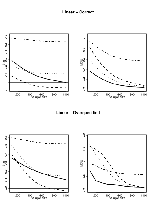
Figure 1: Bias and MSE of the estimated time-varying treatment effect using KOW (solid), IPTW (dashed), sIPTW (dotted) and CBPS (dashed-dotted) when increasing the sample size from $n=100$ to $n=1{,}000$ in the linear-correct scenario (top panels) and in the linear-overspecified scenario (bottom panels).

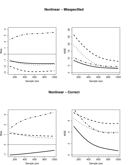
Figure 2: Bias and MSE of the estimated time-varying treatment effect using KOW (solid), IPTW (dashed), sIPTW (dotted) and CBPS (dashed-dotted) when increasing the sample size from $n=100$ to $n=1{,}000$, in the nonlinear-misspecified scenario (top panels) and in the nonlinear-correct scenario (bottom panels).

5.2.2 Across values of the penalization parameter, $\lambda$

Figures 3 and 4 show the ratios of squared biases (left panels) and of MSEs (right panels) when comparing KOW with IPTW (solid), sIPTW (dashed) and CBPS (dotted) across different values of $\lambda$ and $n=500$ in the linear and nonlinear scenarios, respectively. Values above 1 means that KOW had a lower bias or MSE. For zero or small $\lambda$, KOW significantly outperformed IPTW, sIPTW and CBPS with respect to bias. In many cases, the MSE was also smaller for zero $\lambda$. But, the biggest benefit in MSE was seen for larger $\lambda$. The peaks of the right panels represent the points for which $\lambda$ is optimal, i.e., the MSE of KOW is minimized. The solid vertical lines on the right panels show the mean values across replications of the $\lambda$ value obtained by the procedure described in Section 4 and 5.1 as done in the previous section. It can be seen that these are very near the points at which the MSE is minimized. The benefit in MSE both at and around this point was significant across all scenarios.

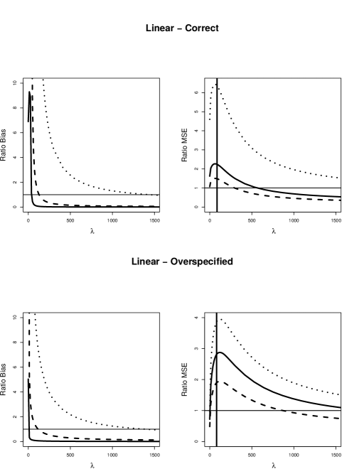
Figure 3: Ratios of squared biases and MSEs comparing KOW with IPTW (solid), sIPTW (dashed) and CBPS (dotted) across values of $\lambda=0,\ldots,1500$ in the linear-correct scenario (top panels) and in the linear-overspecified scenario (bottom panels). Ratios above 1 means that KOW had a lower bias or MSE. Vertical bars show the mean value of $\lambda$, across simulations, obtained as described in Section 5.2.1.

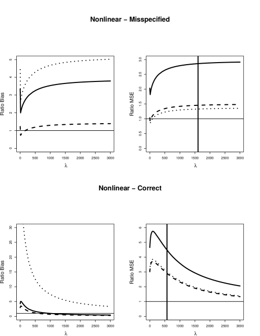
Figure 4: Ratios of squared biases and MSEs comparing KOW with IPTW (solid), sIPTW (dashed) and CBPS (dotted) across values of $\lambda=0,\ldots,3{,}000$ in the nonlinear-misspecified scenario (top panels) and in the nonlinear-correct scenario (bottom panels). Ratios above 1 means that KOW had a lower bias or MSE. Vertical bars show the mean value of $\lambda_{=}0,\ldots,3{,}000$, across simulations, obtained as described in Section 5.2.1.

5.2.3 Computational time of KOW

In this section we present the results of a simulation study aimed at comparing the mean computational time of KOW and CBPS. Compared to sIPTW based on pooled logistic regression, which is generally very fast, both KOW and CBPS have a nontrivial computational time that can grow with both the total number time periods $T$ and the number of covariates (which, for KOW, manifests as the complexity of the kernel functions). For KOW, the most time-consuming tasks are tuning $\lambda$ by marginal likelihood and computing the matrices that define problem (12), which are affected by these two factors, while solving problem (12) is fast and does not depend on those factors. CBPS computational time is dominated by inverting a covariance matrix with dimensions increasing exponentially in $T$ and linearly in the number of covariates. Imai and Ratkovic (2015) also propose using an approximate low-rank matrix that ignores certain covariance terms to make the matrix inversion faster.

Here we compare KOW, CBPS with full covariance matrix (CBPS-full), and CBPS with its low-rank approximation (CBPS-approx) when increasing the number of time periods and the number of covariates. Specifically, following the linear-correct scenario presented in Section 5.1, we fixed the sample size equal to $n=100$ and randomly generated 100 samples considering $T=3,\ldots,10$, and $p=3,\ldots,8$, where $p$ is the total number of covariates $X_{t}$ for each $t$. We fixed the number of covariates to be equal to $p=3$ when evaluating the mean computational times over time periods, while we fixed the number of time periods to be equal to $T=5$ when analyzing over the number of covariates. For each sample, we computed the KOW weights by solving eq. (12) using kernel $\mathcal{K}_{1}$. We used Gaussian process marginal likelihood to tune the kernels’ hyperparameters and penalization parameter. We computed CBPS weights using the linear CBPS as in Section 5.1. We used the R package rbenchmark to compute the computational time on a PC with an i7-3770 processor, 3.4 GHz, 8GB RAM and a Linux Ubuntu 16.04 operating system.

Solid lines of Figure 5 represent mean computational times for KOW, dashed for CBPS-full, and dotted for CBPS-approx. When the number of time periods was relatively small, the mean computational time of KOW was higher compared with both CBPS methods (left panel of Figure 5). However, the mean computation time of KOW over time periods increased linearly while that of both CBPS methods increased exponentially. This is due to the fact that, as presented in Section 3.1, the number of imbalances that we need to minimize grows linearly in the number of time periods. The mean computational time required by KOW when increasing the number of covariates remained constant, while it increased for both CBPS-full and CBPS-approx, with CBPS-full increasing more rapidly. In summary, KOW was less affected by the total number of time periods and covariates compared with CBPS with full and low-rank approximation matrix.

Computing KOW required three steps: tuning the parameters, constructing the matrices for problem (12), and solving problem (12). On average, for $T=3$, the first step required 21% of the total computational time, the second 78.8%, and the last 0.2%. Thus, solving the optimization problem itself is very fast and is not the bottleneck.

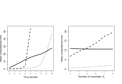
Figure 5: Mean computational time in seconds of KOW (solid), CBPS with full covariate matrix (dashed), and CBPS with the low-rank approximation of the full matrix (dotted) over time periods when $n=100$, $p=3$ and $T=2,\ldots,10$ (left panel) and over number of covariates, when $n=100$, $T=5$ and $p=3,\ldots,8$ (right panel).

6 KOW with informative censoring

In longitudinal studies, participants may drop out the study before the end of the follow-up time and their outcomes are, naturally, missing observations. When this missingness is due to reasons related to the study (i.e., related to the potential outcomes), selection bias is introduced. This phenomenon is referred to as informative censoring and it is common in the context of survival analysis where the interest is on analyzing time-to-event outcomes. Under the assumptions of consistency, positivity, and sequential ignorability of both treatment and censoring, Robins et al. (1999) showed that a consistent estimate of the causal effect of a time-varying treatment can be obtained by weighting each subject $i=1,\ldots,n$ at each time period by the product of inverse probability of treatment and censoring weights. Inverse probability of treatment weights are obtained as presented in Section 2, while inverse probability of censoring weights are usually obtained by inverting the probability of being uncensored at time $t$, given the treatment and confounder history up to time $t$ (Hernán et al., 2001).

In this section we extend KOW to similarly handle informative censoring. We demonstrate that under sequentially ignorable censoring, minimizing the very same discrepancies as before at each time period, restricted to the units for which data is available, actually controls for both time-dependent confounding as well as informative censoring. Thus, KOW naturally extends to the setting with informative censoring.

Let $C_{it}\in\{0,1\}$ for $t=1,\dots,T$ indicate whether unit $i$ is censored in time period $t$ and let $C_{i0}=0$. Note that $C_{it}=1$ implies that $C_{i,t+1}=1$ and that $C_{it}=0$ implies that $C_{i,t-1}=0$. All we require is that we (at least) observe outcomes $Y_{i}$ whenever $C_{iT}=0$, $X_{it}$ whenever $C_{i,t-1}=0$, and $A_{it}$ whenever $C_{it}=0$. Note we might observe more, such as the treatment at time $t$ for a unit with $C_{i,t-1}=0$, or perhaps only some of the data after censoring is corrupted, but that is not required. We summarize the assumption of sequentially ignorable censoring as

$$Y(\overline{a})\mathchoice{\mathrel{\hbox to0.0pt{$\displaystyle\perp$\hss}\mkern 2.0mu{\displaystyle\perp}}}{\mathrel{\hbox to0.0pt{$\textstyle\perp$\hss}\mkern 2.0mu{\textstyle\perp}}}{\mathrel{\hbox to0.0pt{$\scriptstyle\perp$\hss}\mkern 2.0mu{\scriptstyle\perp}}}{\mathrel{\hbox to0.0pt{$\scriptscriptstyle\perp$\hss}\mkern 2.0mu{\scriptscriptstyle\perp}}}\overline{C}_{t}\mid\overline{A}_{t},\overline{X}_{t}.$$ (13)

Let us redefine

$$\delta^{(1)}_{a_{1}}(W,h^{(1)}) =\mathbbm{E}\left[W\mathbbm{1}[A_{1}=a_{1}]\mathbbm{1}[C_{1}=0]h^{(1)}(X_{1})\right]-\mathbbm{E}\left[h^{(1)}(X_{1})\right]$$ (14)

$$g_{\overline{a}}^{(1)}(X_{1}) =\mathbbm{E}\left[Y(\overline{a})\mid X_{1}\right],$$

$$\delta^{(t)}_{a_{t}}(W,h^{(t)}) =\mathbbm{E}\left[W\mathbbm{1}[A_{t}=a_{t}]\mathbbm{1}[C_{t}=0]h^{(t)}(\overline{A}_{t-1},\overline{X}_{t})\right]$$

$$\phantom{=}-\mathbbm{E}\left[W\mathbbm{1}[C_{t-1}=0]h^{(t)}(\overline{A}_{t-1},\overline{X}_{t})\right], \forall t\geq 2,$$

$$g_{\overline{a}}^{(t)}(\overline{A}_{t-1},\overline{X}_{t}) =\mathbbm{1}[\overline{A}_{t-1}=\overline{a}_{t-1}]\mathbbm{E}\left[Y(\overline{a})\mid\overline{A}_{t-1},\overline{X}_{t}\right], \forall t\geq 2.$$

Similarly to Theorem 1, the following theorem shows that we can write the difference between the weighted average outcome among the uncensored $\overline{a}$-treated units, $\mathbbm{E}\left[W\mathbbm{1}[\overline{A}=\overline{a}]\mathbbm{1}[C_{T}=0]Y\right]$, and the true average potential outcome of $\overline{a}$, $\mathbbm{E}\left[Y(\overline{a})\right]$, as the sum over time points $t$ of discrepancies involving the values of treatment and confounder histories up to time $t$.

Theorem 3.

Under assumptions (1)–(2) and (13),

$$\mathbbm{E}\left[W\mathbbm{1}[\overline{A}=\overline{a}]\mathbbm{1}[C_{T}=0]Y\right]-\mathbbm{E}\left[Y(\overline{a})\right]=\sum_{t=1}^{T}\delta^{(t)}_{a_{t}}(W,g_{\overline{a}}^{(t)}).$$ (15)

We then define the empirical counterparts to $\delta^{(t)}_{a_{t}}(W,h^{(t)})$ as before in eq. (7) but limit ourselves to uncensored units, as in eq. (14). We similarly define imbalance, $\text{IMB}(W_{1:n};(\overline{g}_{\overline{a}}^{(t)})_{\overline{a}\in\mathcal{A}})$, and the worst case imbalance $\mathcal{B}^{2}(W_{1:n})$, as before in eqs. (8) and (9). Finally, again using kernels to specify norms, we obtain weights that optimally balance covariates to control for time-dependent confounding and account for informative censoring while controlling precision by solving the quadratic optimization problem,

$$\underset{W_{1:n}\in\mathcal{W}}{\min} \frac{1}{2}W_{1:n}^{T}K_{\lambda}^{\circ}W_{1:n}-e^{T}K_{\lambda}W_{1:n},$$ (16)

where $K_{\lambda}^{\circ}=K^{\circ}+2\lambda I$, $K_{\lambda}=K_{1}+2\lambda I$, $K^{\circ}=\sum_{t=1}^{T}K_{t}^{\circ}$, $K_{t}^{\circ}=\sum_{a_{t}\in\{0,1\}}I^{(t)}_{a_{t}}K_{t}I^{(t)}_{a_{t}}$, $K_{t}\in\mathbb{R}^{n\times n}$ is a semidefinite positive matrix defined as $K_{tij}=\mathcal{K}_{t}((\overline{A}_{i,t-1},\overline{X}_{it}),(\overline{A}_{j,t-1},\overline{X}_{jt}))$, $I^{(t)}_{a_{t}}$ is the diagonal matrix with $\mathbb{I}[A_{it}=a_{t}]\mathbb{I}[C_{it}=0]-\mathbb{I}[C_{i,t-1}=0]$ in its $i^{\text{th}}$ diagonal entry (recall $C_{i,0}=0$ for all $i$), and $e$ is the vector of all ones.

7 Applications

In this section, we present two empirical applications of KOW. In the first, we estimate the effect of treatment initiation on time to death among people living with HIV (PLWH). In the second, we evaluate the impact of negative advertising on election outcomes.

7.1 The effect of HIV treatment on time to death

In this section, we analyze data from the Multicenter AIDS Cohort Study (MACS) to study the effect of the initiation time of treatment on time to death among PLWH. Indeed, due to the longitudinal nature of HIV treatment and the presence of time-dependent confounding, MSMs have been widely used to study causal effects in this domain (Hernán et al., 2000, 2001; HIV-Causal Collaboration et al., 2010; HIV-Causal Collaboration, 2011; Lodi et al., 2017, among others). As an example of time-dependent confounding, CD4 cell count, a measurement used to monitor immune defenses in PLWH and to make clinical decisions, is a predictor of both treatment initiation and survival, as well as being itself influenced by prior treatments. Recognizing the censoring in the MACS data, Hernán et al. (2000) showed how to estimate the parameters of the MSM by inverse probability of treatment and censoring weighting (IPTCW).

Here, we apply KOW as proposed in Section 6 to handle both time-dependent confounding and informative censoring while controlling precision. We considered the following potential time-dependent confounders associated with the effect of treatment initiation and the risk of death: CD4 cell count, white blood cell count, red blood cell count, and platelets. We also identified the age at baseline as a potential time-invariant confounding factor. We considered only recently developed HIV treatments, thus, including in the analysis only PLWH that started treatment after 2001. The final sample was comprised of a total of $n=344$ people and 760 visits, with a maximum of $T=8$ visits per person. We considered two sets of KOW weights, either obtained by using a product of (1) two linear kernels, one for the treatment history and one for the confounder history ($\mathcal{K}_{1}$) or (2) a linear kernel for the treatment history and a polynomial kernel of degree 2 for the confounder history ($\mathcal{K}_{2}$). We scaled the covariates related to the treatment and confounder history, and tuned the kernels’ hyperparameters and the penalization parameter by using Gaussian processes marginal likelihood as presented in Section 4. Following previous approaches studying the HIV treatment using IPTCW that modeled treatment and censoring using single time lags (Hernán et al., 2000, 2001, 2002), we included in each kernel the time-invariant confounders, the previous treatment, $A_{t-1}$, and the time-dependent confounders at time $t$, $X_{t}$, instead of the entire histories. As described in Section 4, since we have repeated observations of outcomes, we compute a set of KOW weights by solving the optimization problem (16) for each horizon up to $T$. In addition, as described in Section 4, we constrained the mean of the weights to be equal to one.

We compared the results obtained by KOW with those from IPTCW and stabilized-IPTCW (sIPTCW). The latter sets of weights were obtained by using a logistic regression on the treatment history and the aforementioned time-invariant and time-dependent confounders and using only one time lag for each of the treatment and time-dependent confounders as done in previous approaches studying the HIV treatment using IPTCW (Hernán et al., 2000, 2001, 2002). The numerator of sIPTCW was computed by modeling $h(\overline{A}_{t})$ in eq. (4) with a logistic regression on the treatment history only using one time lag. We modeled the inverse probability of censoring weights similarly. The final sets of IPTCW and sIPTCW weights were obtained by multiplying inverse probability of treatment and censoring weights. We did not compare the results with those of CBPS because it does not handle informative censoring. In particular, CBPS requires a complete $n\times T$ matrix of observed time-dependent confounders, while in the MACS dataset many entries are missing.

We estimated the hazard ratio of the risk of death by using a weighted Cox regression model (Hernán et al., 2000) weighted by KOW, IPTCW, or sIPTCW and using robust standard errors (Freedman, 2006). We used Gurobi and its R interface to solve eq. (16) and obtain the KOW weights, the Matlab package GPML to perform the marginal likelihood estimation of hyperparameters, the R package R.matlab to call MatLab from within R, the R package ipw (van der Wal et al., 2011) to fit the treatment models for IPTCW and sIPTCW, and the R command coxph (with robust variance estimation) to fit the outcome model. It took 13.5 seconds to obtain a solution for KOW. Table 1 summarizes the result of our analysis. Both KOW ($\mathcal{K}_{1}$) and ($\mathcal{K}_{2}$) showed a significant protective effect of HIV treatment on time to death among PLWH. IPTCW showed a similar effect but with lower precision, resulting in a non-significant effect. With similar precision obtained by KOW, sIPTCW showed a non-significant effect of HIV treatment on time to death. Whereas analyses based on IPTCW and sIPTCW lead to non-significant and inconsistent conclusions, the results we obtained by using KOW show that PLWH can benefit from HIV treatment, as shown in independent randomized placebo-controlled trials (Cameron et al., 1998; Hammer et al., 1997).

Table 1: Effect of HIV treatment on time to death.

	KOW		Logistic
	$\mathcal{K}_{1}$	$\mathcal{K}_{2}$	IPTCW	sIPTCW
$\hat{HR}$	0.40*	0.48*	0.14	1.25
SE	(0.30)	(0.28)	(1.15)	(0.30)

• Note: $\hat{HR}$ is the estimated hazard ratio of the effect of HIV treatment initiation on time to death. $SE$ is the estimated robust standard error. Weights were obtained by using, KOW ($\mathcal{K}_{1}$): a product of two linear kernels, one for the treatment history and one for the confounder history; KOW ($\mathcal{K}_{2}$): a product between a linear kernel for the treatment history and a polynomial kernel of degree 2 for the confounder history; IPTCW: a logistic regression on the treatment history and the time-invariant and time-dependent confounders (using only one time lag for each of the treatment and time-dependent confounders); sIPTCW: stabilized IPTCW. * indicates statistical significance at the 0.05 level.

7.2 The impact of negative advertising on election outcomes

In this section, we analyze a subset of the dataset from Blackwell (2013) to estimate the impact of negative advertising on election outcomes. Because of the dynamic and longitudinal nature of the problem and presence of time-dependent confounders, MSMs have been used previously used to study the question (Blackwell, 2013). Specifically, poll numbers are time-dependent confounders as they might both be affected by negative advertising and might also affect future poll numbers. We constructed the subset of the data from Blackwell (2013) by considering the five weeks leading up to each of 114 elections held 2000–2006 (58 US Senate, 56 US gubernatorial). Differently from Section 7.1 in which the outcome was observed at each time period, in this analysis, the binary election outcome was observed only at the end of each five-week trajectory. In addition, all units were uncensored.

We estimated the parameters of two MSMs, the first having separate coefficients for negative advertising in each time period and the second having one coefficient for the cumulative effect of negative advertising. Each MSM was fit using weights given by each of KOW, IPTW, sIPTW, and CBPS (both full and approximate). We used the following time-dependent confounders: Democratic share of the polls, proportion of undecided voters, and campaign length. We also used the following time-invariant confounders: baseline Democratic vote share, proportion of undecided voters, status of incumbency, election year and type of office. We obtained two sets of KOW weights by using a product of (1) two linear kernels, one for the history of negative advertising and one for the confounder history ($\mathcal{K}_{1}$) and (2) a linear kernel for the history of negative advertising and a polynomial kernel of degree 2 for the confounder history ($\mathcal{K}_{2}$). The kernels were over the complete confounder history up to time $t$, $\overline{X}_{t}$, and two time-lags of treatment history, $A_{t-1},A_{t-2}$. We scaled the covariates and tuned the kernels’ hyperparameters and the penalization parameter by using Gaussian processes marginal likelihood. We obtained the final set of KOW weights by solving eq. (12). We compared the results obtained by KOW with those from IPTW, sIPTW, CBPS-full, and CBPS-approx. To obtain the sets of IPTW, sIPTW, and CBPS weights, we used logistic models conditioned on the confounder history and two time-lags from the treatment history. To compute the numerator of sIPTW weights, we used a logistic regression conditioned only on two time-lags from the treatment history. We used Gurobi and its R interface to solve eq. (16) and obtain the KOW weights, the Matlab package GPML to perform the marginal likelihood estimation of hyperparameters, the R package R.matlab to call MatLab from within R, the R command glm to fit the treatment models for IPTW and sIPTW, the R package CBMSM for CBPS, the R command lm to fit the outcome model, and the R package sandwich to estimate robust standard errors. The computational time to obtain a solution was equal to 12.6 seconds for KOW, while it was equal to 104 seconds for CBPS-full and 3.8 seconds for CBPS-approx.

Table 2 summarizes the results of our analysis, reporting robust standard errors (Freedman, 2006). The first six rows of Table 2 show the effect of the time-specific negative advertising. The last two rows present the effect of the cumulative effect of negative advertising. KOW ($\mathcal{K}_{1}$ and $\mathcal{K}_{2}$) and IPTW showed similar effects, with increased precision when using KOW except for time 4, in which both methods showed a significant negative effect but with greater precision when using IPTW. sIPTW, CBPS-full and CBPS-approx showed a significant negative effect at time 3 with similar precision. No significant results were obtained when considering the cumulative effect of negative advertising. All except sIPTW, showed a negative cumulative effect. KOW ($\mathcal{K}_{1}$) was the most precise. We conclude that, the impact of negative advertising in the majority of the time periods and its cumulative effect on election outcomes are not statistically significant.

Table 2: Impact of negative advertising on election outcomes.

$\hat{\beta}$	KOW		Logistic		CBPS
$SE$	$\mathcal{K}_{1}$	$\mathcal{K}_{2}$	IPTW	sIPTW	Full	Approx
Intercept	54.54*	53.84*	53.05*	47.46*	51.25*	52.17*
	(2.15)	(2.38)	(2.88)	(2.98)	(2.70)	(2.39)
Negative1	2.43	3.27	4.41	7.62*	5.95*	4.81*
	(1.86)	(1.86)	(2.56)	(3.26)	(2.49)	(2.22)
Negative2	3.73	3.24	5.51*	3.17	3.55	2.65
	(2.18)	(2.22)	(2.38)	(3.19)	(2.73)	(2.42)
Negative3	-2.51	-2.39	-4.37	-8.32*	-6.50*	-6.31*
	(2.34)	(2.45)	(2.54)	(3.84)	(3.20)	(3.24)
Negative4	-7.16*	-7.22*	-8.77*	2.34	-3.55	-3.12
	(2.57)	(2.75)	(1.54)	(3.11)	(3.71)	(3.59)
Negative5	-2.75*	-1.79	-3.19	-3.62	-1.92	-1.96
	(1.42)	(1.59)	(2.19)	(2.59)	(1.62)	(1.54)
Intercept	51.40*	50.56*	58.29*	42.63*	49.38*	50.28*
	(2.45)	(2.63)	(4.29)	(4.15)	(2.68)	(2.49)
Cumulative	-0.59	-0.37	-0.93	1.91	-0.28	-0.41
	(0.58)	(0.64)	(1.57)	(1.15)	(0.65)	(0.77)

• Note: $\hat{\beta}$ is the estimated effect of negative advertising. $SE$ is the estimated robust standard error. Weights were obtained by using, KOW ($\mathcal{K}_{1}$): a product of two linear kernels, one for the history of negative advertising and one for the confounder history; KOW ($\mathcal{K}_{2}$): a product between a linear kernel for the history of negative advertising and a polynomial kernel of degree 2 for the confounder history; IPTW: a logistic model conditioned on the confounder history and two time-lags from the treatment history; sIPTW: stabilized IPTW; CBPS-full: CBPS with full covariance matrix; CBPS-approx: CBPS with low-rank approximation. * indicates statistical significance at the 0.05 level.

8 Conclusions

In this paper we presented KOW, which optimally finds weights for fitting an MSM with the aim of balancing time-dependent confounders while controlling for precision. That KOW uses mathematical optimization to directly and fully balance covariates as well as optimize precision explains the better performance of KOW over IPTW, sIPTW and CBPS observed in our simulation study. In addition, as shown in Sections 3.2, 5 and 6, the proposed methodology only needs to minimize a number of discrepancies that grows linearly in the number of time periods, mitigates the possible misspecification of the treatment assignment model, allows balancing non-additive covariate relationships, and can be extended to control for informative censoring, which is a common feature of longitudinal studies.

Alternative formulations of our imbalance-precision optimization problem, eq. (10), may be investigated. For example, additional linear constraints can be added to the optimization problem, as shown in the empirical application of Section 7.1, and different penalties can be considered to control for extreme weights. For instance, in eq. (10), at the cost of no longer being able to use convex-quadratic optimization, one may directly penalize the covariance matrix of the weighted least-square estimator rather than use a convex-quadratic surrogate as we do.

One may also change the nature of precision control. Here, we suggested penalization in an attempt to target total error. Alternatively, similar to Santacatterina and Bottai (2018), we may reformulate eq. (10) as a constrained optimization problem where the precision of the resulting estimator is constrained by an upper bound $\xi$, thus seeking to minimize imbalances subject to having a bounded precision. In our convex formulation, the two are equivalent by Lagrangian duality in that for every precision penalization $\lambda$ there is an equivalent precision bound $\xi$. However, it may make specifying the parameters easier depending on the application as it may be easier for a practitioner to conceive of a desirable bound on precision. There may also be other ways to choose the penalization parameter. Here we suggested using maximum marginal likelihood but cross validation based on predicting outcomes and their partial means may also be possible.

The flexibility of our approach is that any of these changes amount to simply modifying the optimization problem that is fed to an off-the-shelf solver. Indeed, we were able to extend KOW from the standard longitudinal setting to also handle both repeated observations of outcomes and informative censoring. In addition to offering flexibility, the optimization approach we took, which directly and fully minimized our error objective phrased in terms of covariate imbalances, was able to offer improvements on the state of the art.

Appendix

Proof of Theorem 1.

For clarity, we prove this for $T=2$. The extension to $T>2$ is by induction. Under consistency and assumptions (1)–(2), we have

$$\mathbb{E}[W\mathbbm{1}[\overline{A}=\overline{a}]Y]$$

$$=\mathbb{E}[W\mathbbm{1}[A_{1}=a_{1}]\mathbbm{1}[A_{2}=a_{2}]Y(\overline{a})]$$ (consistency)

$$=\mathbb{E}[W\mathbbm{1}[A_{1}=a_{1}]\mathbbm{1}[A_{2}=a_{2}]\mathbb{E}[Y(\overline{a})\mid A_{1},A_{2},X_{1},X_{2}]]$$ (iterated expectations)

$$=\mathbb{E}[W\mathbbm{1}[A_{1}=a_{1}]\mathbbm{1}[A_{2}=a_{2}]\mathbb{E}[Y(\overline{a})\mid A_{1},X_{1},X_{2}]]$$ (sequential ignorability)

$$=\mathbb{E}[W\mathbbm{1}[A_{1}=a_{1}]\mathbb{E}[Y(\overline{a})\mid A_{1},X_{1},X_{2}]]+\delta^{(2)}_{\overline{a}}(W,g_{\overline{a}}^{(2)}) \delta^{(2)}_{\overline{a}},g_{\overline{a}}^{(2)}$$ (definition of )

$$=\mathbb{E}[W\mathbbm{1}[A_{1}=a_{1}]\mathbb{E}[Y(\overline{a})\mid A_{1},X_{1}]]+\delta^{(2)}_{\overline{a}}(W,g_{\overline{a}}^{(2)})$$ (iterated expectations)

$$=\mathbb{E}[W\mathbbm{1}[A_{1}=a_{1}]\mathbb{E}[Y(\overline{a})\mid X_{1}]]+\delta^{(2)}_{\overline{a}}(W,g_{\overline{a}}^{(2)})$$ (sequential ignorability)

$$=\mathbb{E}[\mathbb{E}[Y(\overline{a})\mid X_{1}]]+\delta^{(1)}_{\overline{a}}(W,g_{\overline{a}}^{(1)})+\delta^{(2)}_{\overline{a}}(W,g_{\overline{a}}^{(2)}) \delta^{(1)}_{\overline{a}},g_{\overline{a}}^{(1)}$$ (definition of )

$$=\mathbb{E}[Y(\overline{a})]+\delta^{(1)}_{\overline{a}}(W,g_{\overline{a}}^{(1)})+\delta^{(2)}_{\overline{a}}(W,g_{\overline{a}}^{(2)})$$ (iterated expectations)

∎

Proof of Thm. 2.

Define $K_{tij}=\mathcal{K}_{t}((\overline{A}_{i,t-1},\overline{X}_{it}),(\overline{A}_{j,t-1},\overline{X}_{jt}))$. Then, by the representer property of the kernels and by self-duality of Hilbert spaces,

$$\Delta^{(1)}_{a_{1}}(W_{1:n})^{2} =\sup_{\|h^{(1)}\|_{(1)}^{2}\leq 1}\left(\hat{\delta}^{(1)}_{a_{1}}(W_{1:n},h^{(1)})\right)^{2}$$

$$=\text{sup}_{\|h^{(1)}\|^{2}_{(1)}\leq 1}\left(\dfrac{1}{n}\sum_{i=1}^{n}\underbrace{\left(W_{i}\mathbbm{1}[A_{t}=a_{t}]-1\right)}_{z_{i}}h^{(1)}(X_{i1})\right)^{2}$$

$$=\text{sup}_{\|h^{(1)}\|^{2}_{(1)}\leq 1}\left(\dfrac{1}{n}\sum_{i=1}^{n}z_{i}\langle\mathcal{K}_{t}((X_{i1}),\cdot),h^{(1)}(X_{i1})\rangle\right)^{2}$$

$$=\left\|\dfrac{1}{n}\sum_{i=1}^{n}z_{i}\mathcal{K}_{1}((X_{i1}),\cdot)\right\|_{(1)}^{2}$$

$$=\left\langle\dfrac{1}{n}\sum_{i=1}^{n}z_{i}\mathcal{K}_{t}((X_{i1}),\cdot),\dfrac{1}{n}\sum_{i=1}^{n}z_{i}\mathcal{K}_{t}((X_{i1}),\cdot)\right\rangle$$

$$=\dfrac{1}{n^{2}}\sum_{i=1}^{n}\sum_{j=1}^{n}z_{i}z_{j}\mathcal{K}_{t}((X_{i1}),(X_{j1}))$$

$$=\frac{1}{n^{2}}\sum_{i=1}^{n}\sum_{j=1}^{n}(W_{i}\mathbb{I}[A_{i1}=a_{1}]-1)(W_{j}\mathbb{I}[A_{j1}=a_{1}]-1)K_{tij}$$

$$=\frac{1}{n^{2}}(I^{(1)}_{a_{1}}W_{1:n}-e)^{T}K_{t}(I^{(1)}_{a_{1}}W_{1:n}-e)$$

$$=\frac{1}{n^{2}}W_{1:n}^{T}I^{(1)}_{a_{1}}K_{1}I^{(1)}_{a_{1}}W_{1:n}-2e^{T}K_{1}I^{(1)}_{a_{1}}W_{1:n}+e^{T}K_{1}e$$

$$\Delta^{(t)}_{a_{t}}(W_{1:n})^{2} =\sup_{\|h^{(t)}\|_{(t)}^{2}\leq 1}\left(\hat{\delta}^{(t)}_{a_{t}}(W_{1:n},h^{(t)})\right)^{2}$$

$$=\text{sup}_{\|h^{(t)}\|^{2}_{(t)}\leq 1}\left(\dfrac{1}{n}\sum_{i=1}^{n}\underbrace{\left(\mathbbm{1}[A_{t}=a_{t}]-1\right)W_{i}}_{z_{i}}h^{(t)}(\overline{A}_{i,t-1},\overline{X}_{it})\right)^{2}$$

$$=\text{sup}_{\|h^{(t)}\|^{2}_{(t)}\leq 1}\left(\dfrac{1}{n}\sum_{i=1}^{n}z_{i}\langle\mathcal{K}_{t}((\overline{A}_{i,t-1},\overline{X}_{it}),\cdot),h^{(t)}(\overline{A}_{i,t-1},\overline{X}_{it})\rangle\right)^{2}$$

$$=\left\|\dfrac{1}{n}\sum_{i=1}^{n}z_{i}\mathcal{K}_{t}((\overline{A}_{i,t-1},\overline{X}_{it}),\cdot)\right\|_{(t)}^{2}$$

$$=\left\langle\dfrac{1}{n}\sum_{i=1}^{n}z_{i}\mathcal{K}_{t}((\overline{A}_{i,t-1},\overline{X}_{it}),\cdot),\dfrac{1}{n}\sum_{i=1}^{n}z_{i}\mathcal{K}_{t}((\overline{A}_{i,t-1},\overline{X}_{it}),\cdot)\right\rangle$$

$$=\dfrac{1}{n^{2}}\sum_{i=1}^{n}\sum_{j=1}^{n}z_{i}z_{j}\mathcal{K}_{t}((\overline{A}_{i,t-1},\overline{X}_{it}),(\overline{A}_{j,t-1},\overline{X}_{jt}))$$

$$=\frac{1}{n^{2}}\sum_{i=1}^{n}\sum_{j=1}^{n}(W_{i}\mathbb{I}[A_{it}=a_{t}]-W_{i})(W_{j}\mathbb{I}[A_{jt}=a_{t}]-W_{j})K_{tij}$$

$$=\frac{1}{n^{2}}(I^{(t)}_{a_{t}}W_{1:n}-W_{1:n})^{T}K_{t}(I^{(t)}_{a_{t}}W_{1:n}-W_{1:n})$$

$$=\frac{1}{n^{2}}W_{1:n}^{T}(I-I^{(t)}_{a_{t}})K_{t}(I-I^{(t)}_{a_{t}})W_{1:n}$$

∎

Proof of Theorem 3.

For clarity, we prove this for $T=2$. The extension to $T>2$ is by induction. Under consistency, assumptions (1)–(2), and assumption (13),

$$\mathbb{E}[W\mathbbm{1}[\overline{A}=\overline{a}]\mathbbm{1}[C_{2}=0]Y]$$

$$=\mathbb{E}[W\mathbbm{1}[A_{1}=a_{1}]\mathbbm{1}[A_{2}=a_{2}]\mathbbm{1}[C_{2}=0]Y(\overline{a})]$$ (consistency)

$$=\mathbb{E}[W\mathbbm{1}[A_{1}=a_{1}]\mathbbm{1}[A_{2}=a_{2}]\mathbbm{1}[C_{2}=0]\mathbb{E}[Y(\overline{a})\mid A_{1},A_{2},X_{1},X_{2},C_{2},C_{1}]]$$ (iterated expectations)

$$=\mathbb{E}[W\mathbbm{1}[A_{1}=a_{1}]\mathbbm{1}[A_{2}=a_{2}]\mathbbm{1}[C_{2}=0]\mathbb{E}[Y(\overline{a})\mid A_{1},A_{2},X_{1},X_{2}]]$$ (eq. (13))

$$=\mathbb{E}[W\mathbbm{1}[A_{1}=a_{1}]\mathbbm{1}[A_{2}=a_{2}]\mathbbm{1}[C_{2}=0]\mathbb{E}[Y(\overline{a})\mid A_{1},X_{1},X_{2}]]$$ (eq. (2))

$$=\mathbb{E}[W\mathbbm{1}[A_{1}=a_{1}]\mathbbm{1}[C_{1}=0]\mathbb{E}[Y(\overline{a})\mid A_{1},X_{1},X_{2}]]+\delta^{(2)}_{\overline{a}}(W,g_{\overline{a}}^{(2)}) \delta^{(2)}_{\overline{a}},g_{\overline{a}}^{(2)}$$ (definition of )

$$=\mathbb{E}[W\mathbbm{1}[A_{1}=a_{1}]\mathbbm{1}[C_{1}=0]\mathbb{E}[Y(\overline{a})\mid A_{1},A_{2},X_{1},X_{2}]]+\delta^{(2)}_{\overline{a}}(W,g_{\overline{a}}^{(2)})$$ (eq. (2))

$$=\mathbb{E}[W\mathbbm{1}[A_{1}=a_{1}]\mathbbm{1}[C_{1}=0]\mathbb{E}[Y(\overline{a})\mid A_{1},A_{2},X_{1},X_{2},C_{1},C_{2}]]+\delta^{(2)}_{\overline{a}}(W,g_{\overline{a}}^{(2)})$$ (eq. (13))

$$=\mathbb{E}[W\mathbbm{1}[A_{1}=a_{1}]\mathbbm{1}[C_{1}=0]\mathbb{E}[Y(\overline{a})\mid A_{1},X_{1},C_{1}]]+\delta^{(2)}_{\overline{a}}(W,g_{\overline{a}}^{(2)})$$ (iterated expectations)

$$=\mathbb{E}[W\mathbbm{1}[A_{1}=a_{1}]\mathbbm{1}[C_{1}=0]\mathbb{E}[Y(\overline{a})\mid A_{1},X_{1}]]+\delta^{(2)}_{\overline{a}}(W,g_{\overline{a}}^{(2)})$$ (eq. (13))

$$=\mathbb{E}[W\mathbbm{1}[A_{1}=a_{1}]\mathbbm{1}[C_{1}=0]\mathbb{E}[Y(\overline{a})\mid X_{1}]]+\delta^{(2)}_{\overline{a}}(W,g_{\overline{a}}^{(2)})$$ (eq. (2))

$$=\mathbb{E}[\mathbbm{1}[C_{0}=0]\mathbb{E}[Y(\overline{a})\mid X_{1}]]+\delta^{(1)}_{\overline{a}}(W,g_{\overline{a}}^{(1)})+\delta^{(2)}_{\overline{a}}(W,g_{\overline{a}}^{(2)}) \delta^{(1)}_{\overline{a}},g_{\overline{a}}^{(1)}$$ (definition of )

$$=\mathbb{E}[Y(\overline{a})]+\delta^{(1)}_{\overline{a}}(W,g_{\overline{a}}^{(1)})+\delta^{(2)}_{\overline{a}}(W,g_{\overline{a}}^{(2)})$$ (iterated expectations)

∎

References

- Berlinet and Thomas-Agnan (2011) Berlinet, A. and C. Thomas-Agnan (2011). Reproducing kernel Hilbert spaces in probability and statistics. Springer Science & Business Media.
- Blackwell (2013) Blackwell, M. (2013). A framework for dynamic causal inference in political science. American Journal of Political Science 57(2), 504–520.
- Cameron et al. (1998) Cameron, D. W., M. Heath-Chiozzi, S. Danner, C. Cohen, S. Kravcik, C. Maurath, E. Sun, D. Henry, R. Rode, A. Potthoff, et al. (1998). Randomised placebo-controlled trial of ritonavir in advanced hiv-1 disease. The Lancet 351(9102), 543–549.
- Cole and Hernán (2008) Cole, S. R. and M. A. Hernán (2008). Constructing inverse probability weights for marginal structural models. American journal of epidemiology 168(6), 656–664.
- D’Agostino et al. (1990) D’Agostino, R. B., M.-L. Lee, A. J. Belanger, L. A. Cupples, K. Anderson, and W. B. Kannel (1990). Relation of pooled logistic regression to time dependent cox regression analysis: the framingham heart study. Statistics in medicine 9(12), 1501–1515.
- Freedman (2006) Freedman, D. A. (2006). On the so-called “huber sandwich estimator” and “robust standard errors”. The American Statistician 60(4), 299–302.
- Gruber et al. (2015) Gruber, S., R. W. Logan, I. Jarrín, S. Monge, and M. A. Hernán (2015). Ensemble learning of inverse probability weights for marginal structural modeling in large observational datasets. Statistics in medicine 34(1), 106–117.
- Gurobi Optimization (2018) Gurobi Optimization (2018). Gurobi optimizer reference manual.
- Hammer et al. (1997) Hammer, S. M., K. E. Squires, M. D. Hughes, J. M. Grimes, L. M. Demeter, J. S. Currier, J. J. Eron Jr, J. E. Feinberg, H. H. Balfour Jr, L. R. Deyton, et al. (1997). A controlled trial of two nucleoside analogues plus indinavir in persons with human immunodeficiency virus infection and cd4 cell counts of 200 per cubic millimeter or less. New England Journal of Medicine 337(11), 725–733.
- Hernán et al. (2008) Hernán, M. A., A. Alonso, R. Logan, F. Grodstein, K. B. Michels, M. J. Stampfer, W. C. Willett, J. E. Manson, and J. M. Robins (2008). Observational studies analyzed like randomized experiments: an application to postmenopausal hormone therapy and coronary heart disease. Epidemiology (Cambridge, Mass.) 19(6), 766.
- Hernán et al. (2000) Hernán, M. Á., B. Brumback, and J. M. Robins (2000). Marginal structural models to estimate the causal effect of zidovudine on the survival of hiv-positive men. Epidemiology 11(5), 561–570.
- Hernán et al. (2001) Hernán, M. A., B. Brumback, and J. M. Robins (2001). Marginal structural models to estimate the joint causal effect of nonrandomized treatments. Journal of the American Statistical Association 96(454), 440–448.
- Hernán et al. (2002) Hernán, M. A., B. A. Brumback, and J. M. Robins (2002). Estimating the causal effect of zidovudine on cd4 count with a marginal structural model for repeated measures. Statistics in medicine 21(12), 1689–1709.
- Hernán and Robins (2010) Hernán, M. A. and J. M. Robins (2010). Causal inference. CRC Boca Raton, FL:.
- HIV-Causal Collaboration (2011) HIV-Causal Collaboration (2011). When to initiate combined antiretroviral therapy to reduce mortality and AIDS-defining illness in HIV-infected persons in developed countries: an observational study. Annals of Internal Medicine 154(8), 509.
- HIV-Causal Collaboration et al. (2010) HIV-Causal Collaboration et al. (2010). The effect of combined antiretroviral therapy on the overall mortality of hiv-infected individuals. AIDS (London, England) 24(1), 123.
- Imai and Ratkovic (2014) Imai, K. and M. Ratkovic (2014). Covariate balancing propensity score. Journal of the Royal Statistical Society: Series B (Statistical Methodology) 76(1), 243–263.
- Imai and Ratkovic (2015) Imai, K. and M. Ratkovic (2015). Robust estimation of inverse probability weights for marginal structural models. Journal of the American Statistical Association 110(511), 1013–1023.
- Imbens and Rubin (2015) Imbens, G. W. and D. B. Rubin (2015). Causal inference in statistics, social, and biomedical sciences. Cambridge University Press.
- Kallus (2016) Kallus, N. (2016). Generalized optimal matching methods for causal inference. arXiv preprint arXiv:1612.08321.
- Kallus (2018) Kallus, N. (2018). Optimal a priori balance in the design of controlled experiments. Journal of the Royal Statistical Society: Series B (Statistical Methodology) 80(1), 85–112.
- Kallus et al. (2018) Kallus, N., B. Pennicooke, and M. Santacatterina (2018). More robust estimation of sample average treatment effects using kernel optimal matching in an observational study of spine surgical interventions. arXiv preprint arXiv:1811.04274.
- Kang and Schafer (2007) Kang, J. D. and J. L. Schafer (2007). Demystifying double robustness: A comparison of alternative strategies for estimating a population mean from incomplete data. Statistical science, 523–539.
- Karim et al. (2017) Karim, M. E., J. Petkau, P. Gustafson, H. Tremlett, and T. B. S. Group (2017). On the application of statistical learning approaches to construct inverse probability weights in marginal structural cox models: Hedging against weight-model misspecification. Communications in Statistics-Simulation and Computation, 1–30.
- Karim and Platt (2017) Karim, M. E. and R. W. Platt (2017). Estimating inverse probability weights using super learner when weight-model specification is unknown in a marginal structural cox model context. Statistics in Medicine 36(13), 2032–2047.
- Lefebvre et al. (2008) Lefebvre, G., J. A. Delaney, and R. W. Platt (2008). Impact of mis-specification of the treatment model on estimates from a marginal structural model. Statistics in medicine 27(18), 3629–3642.
- Lodi et al. (2017) Lodi, S., D. Costagliola, C. Sabin, J. del Amo, R. Logan, S. Abgrall, P. Reiss, A. van Sighem, S. Jose, J.-r. Blanco, et al. (2017). Effect of immediate initiation of antiretroviral treatment in hiv-positive individuals aged 50 years or older. Jaids Journal of Acquired Immune Deficiency Syndromes.
- Rasmussen and Nickisch (2010) Rasmussen, C. E. and H. Nickisch (2010). Gaussian processes for machine learning (gpml) toolbox. Journal of Machine Learning Research 11(Nov), 3011–3015.
- Rasmussen and Williams (2006) Rasmussen, C. E. and C. K. Williams (2006). Gaussian processes for machine learning, Volume 1. MIT press Cambridge.
- Robins (2000) Robins, J. M. (2000). Marginal structural models versus structural nested models as tools for causal inference. In Statistical models in epidemiology, the environment, and clinical trials, pp. 95–133. Springer.
- Robins et al. (1999) Robins, J. M., S. Greenland, and F.-C. Hu (1999). Estimation of the causal effect of a time-varying exposure on the marginal mean of a repeated binary outcome. Journal of the American Statistical Association 94(447), 687–700.
- Robins et al. (2000) Robins, J. M., M. A. Hernan, and B. Brumback (2000). Marginal structural models and causal inference in epidemiology. Epidemiology 11(5), 550–560.
- Robins et al. (1995) Robins, J. M., A. Rotnitzky, and L. P. Zhao (1995). Analysis of semiparametric regression models for repeated outcomes in the presence of missing data. Journal of the american statistical association 90(429), 106–121.
- Rosenbaum and Rubin (1983) Rosenbaum, P. R. and D. B. Rubin (1983). The central role of the propensity score in observational studies for causal effects. Biometrika 70(1), 41–55.
- Rubin (1980) Rubin, D. B. (1980). Randomization analysis of experimental data: The fisher randomization test comment. Journal of the American Statistical Association 75(371), 591–593.
- Santacatterina and Bottai (2018) Santacatterina, M. and M. Bottai (2018). Optimal probability weights for inference with constrained precision. Journal of the American Statistical Association 113(523), 983–991.
- Santacatterina et al. (2019) Santacatterina, M., C. García-Pareja, R. Bellocco, A. Sönnerborg, A. M. Ekström, and M. Bottai (2019). Optimal probability weights for estimating causal effects of time-varying treatments with marginal structural cox models. Statistics in medicine 38(10), 1891–1902.
- Scharfstein et al. (1999) Scharfstein, D. O., A. Rotnitzky, and J. M. Robins (1999). Adjusting for nonignorable drop-out using semiparametric nonresponse models. Journal of the American Statistical Association 94(448), 1096–1120.
- Schölkopf and Smola (2002) Schölkopf, B. and A. J. Smola (2002). Learning with kernels: support vector machines, regularization, optimization, and beyond. MIT press.
- van der Wal et al. (2011) van der Wal, W. M., R. B. Geskus, et al. (2011). Ipw: an r package for inverse probability weighting. J Stat Softw 43(13), 1–23.
- Xiao et al. (2013) Xiao, Y., E. E. Moodie, and M. Abrahamowicz (2013). Comparison of approaches to weight truncation for marginal structural cox models. Epidemiologic Methods 2(1), 1–20.