SuMo-SS: Submodular Optimization Sensor Scattering for
Deploying Sensor Networks by Drones
Abstract
To meet the immediate needs of environmental monitoring or hazardous event detection, we consider the automatic deployment of a group of low-cost or disposable sensors by a drone. Introducing sensors by drones to an environment instead of humans has advantages in terms of worker safety and time requirements. In this study, we define “sensor scattering (SS)” as the problem of maximizing the information-theoretic gain from sensors scattered on the ground by a drone. SS is challenging due to its combinatorial explosion nature, because the number of possible combination of sensor positions increases exponentially with the increase in the number of sensors.
In this paper, we propose an online planning method called SubModular Optimization Sensor Scattering (SuMo-SS). Unlike existing methods, the proposed method can deal with uncertainty in sensor positions. It does not suffer from combinatorial explosion but obtains a –approximation of the optimal solution. We built a physical drone that can scatter sensors in an indoor environment as well as a simulation environment based on the drone and the environment. In this paper, we present the theoretical background of our proposed method and its experimental validation.
I Introduction
Low-cost or disposable wireless sensors have a huge potential impact on environmental monitoring and hazardous event detection. In this study, we consider the problem of the automatic deployment of sensor networks using a drone. Typical use cases include monitoring flash floods in a desert[1], human detection in landslides, and contamination detection on a mountain.
In most of such applications, humans are not supposed to enter the target area because of safety, cost, or other reasons; therefore, unmanned sensor deployment is required. In this paper, we use a drone to transport sensors to a target area to monitor it. Because most drones have limited battery resources, careful planning for their transportation is required to maximize a certain information-theoretic gain.
In this paper, we define a sensor scattering (SS) problem as a planning problem where drones scatter sensors in a target area to maximize a certain information criterion. In an SS problem, we have to consider the following two issues. First, because sensors are dropped from the air, their final positions on the ground are uncertain depending on the terrain and their construction material. Second, it is reasonable to update the plan online because of uncertainty in sensor positions.
The SS problem has a close relationship with the sensor placement problem[2]. Both problems are challenging because they are typically NP-hard[3]. The number of possible combinations of sensors increases exponentially as the number of sensors increases. Recently, Krause’s work[4] proved that –approximation can be obtained using submodularity in the mutual information criterion. This means that 63% of the optimal score is guaranteed using a greedy method, which can avoid a combinatorial explosion. However, the method assumes that the sensor positions are known, which is invalid in SS problems.
In this paper, we propose an SS method that plans sensor positions in an online manner. It does not suffer from combinatorial explosion but obtains a –approximation of the optimal solution. A typical task scenario is illustrated in Figure1. We built a customized physical drone that could scatter sensors in an indoor environment in addition to a simulation environment. In this paper, we present the theoretical background of our proposed method and its experimental validation. To make the experimental results reproducible, the experiments were performed in the simulated environment shown in Figure4.
The following is our key contribution:
-
•
We propose the SubModular Optimization Sensor Scattering (SuMo-SS) method that considers distance-based uncertainty in sensor positions, which is relevant for practical applications. The method is explained in Section V.
II Related Work
There have been many studies on sensor placement, especially in the fields of sensor networks and robotics[3, 5, 6, 2]. For readability, we use the term “drone” instead of “Unmanned Aerial Vehicle (UAV)” or “multiroter helicopter”.
Research on optimized node placement in wireless sensor networks was previously summarized in [3]. Some recent studies used drones for deploying sensors for optimal topology[7] or connectivity[8]. In [1], low-cost sensors were scattered from a drone and used for detecting a flash flood; however, the work did not discuss how to optimally scatter the sensors.
In the wireless sensor network community, drone-based monitoring has been investigated to improve quality of user experience (QoE)[9]. A method to minimize a cost function based on a cover function was proposed in [9]. Energy-efficient 3D placement of a drone that maximizes the number of covered users using the minimum required transmit power was proposed in [10].
Uncertainty in positions, poses and maps have been widely investigated in path planning and simultaneous localization and mapping (SLAM) studies[11]. In [12], a path planning method for mobile robots based on expected uncertainty reduction was proposed. Uncertainty in the maps and poses was modeled with a Rao-Blackwellized particle filter. Sim and Roy proposed a path planning method based on an active learning approach utilizing A-optimality[13]. In other studies, the path was planned to maximize a certain information-theoretic gain of sensors mounted on drones[14].
The first attempt that introduced submodularity in path planning was done in [15]. Singh et al. also proposed a path planning method utilizing submodularity, and conducted real-world experiments with river- and lake-monitoring robots[16]. The submodularity objective proposed in [17] included sensor failure and a penalty reduction for the worst case. Their target application included the detection of contamination in a large water distribution network. Golovin et al. proposed the concept of adaptive submodularity in order to extend the optimization policy from a greedy method to adaptive policies[18]. In their work, uncertainty in sensor failure was discussed. However, none of the above studies discussed uncertainty in sensor positions.
Submodularity has a close relationship with the combinatorial theory of matroids. Williams et al. recently proposed to model multi-robot tasks as functionality-requirement pairs, and applied a matroid optimization method to task allocation[19]. In their model, no uncertainty was handled. Specifically, unlike our method, their method does not consider uncertainty in sensor positions.
There have also been many attempts on alternative sensor placement methods such as evolutionary computation[20]. The method proposed in [21] can handle uncertainty in line-of-sight coverage, however it cannot handle uncertainty in sensor positions. Moreover, the method cannot be applicable to an SS problem because online planning is impossible. Indeed, most evolutionary algorithms suffer from the fact that the learning cannot be conducted in an online manner.
Recently, drone-based monitoring has been extended to sound source localization. In [22], a microphone array equipped to a drone was used for robustly localizing sound sources on the ground. Nakadai et al. proposed an online outdoor sound source localization method and evaluated it with a microphone array embedded on a drone[23].
III Problem Statement and Task Scenario
In this paper, we define an SS problem as follows:
-
•
A planning problem in which drones scatter sensors in a target area to maximize a certain information criterion.
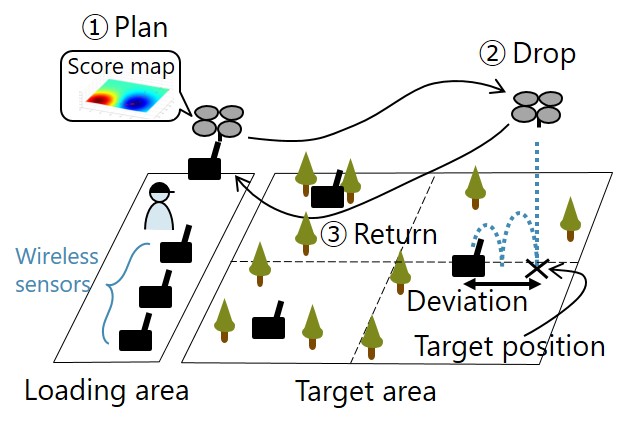
A typical task scenario of SS is illustrated in Figure1. SS is an online planning problem based on uncertain information. Previously scattered sensors affect the position of subsequent sensors, and actual sensor positions might deviate from their planned positions. In this paper, we define the term “deviation” as follows:
-
•
The distance between the positions at which the drone drops the sensor and at which it lands. Although we are only considering two-dimensional deviation and distance, the method is not limited in dimensionality. In this paper, the distance is simply projected on the ground.
The following are the input and output of the planning method:
- Input
-
: Covariance between previously scattered sensors and their target positions
- Output
-
: Target position of the next sensor and its informational gain
The target area is defined as the area to be monitored by the sensors. Humans are not supposed to enter it.
The task scenario is summarized as follows:
-
(0)
Initialization: The drone takes off from the loading area. While the drone is hovering, the experimenter attaches a sensor to it. Although it could be autonomously loaded by the drone, that idea is outside the scope of this study.
-
(1)
Plan: Given the previously scattered sensors, target position is planned by our method.
-
(2)
Drop: The drone flies to and drops the sensor. The actual sensor position on the ground, is randomly deviated from .
-
(3)
Return: The drone returns to the loading position, and loads the next sensor. Go to Step (1) until the maximum number of sensors have been placed.
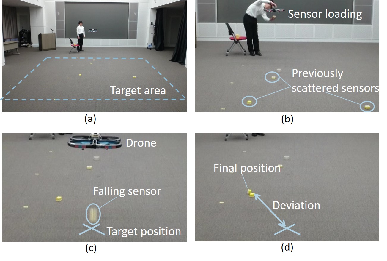
Demo video clip is available at this website111https://youtu.be/cLx9_Zv10Oo.
We assume that no remote control is performed by humans; therefore, the drone must navigate itself based on its sensor observations and a known map. Indeed in our experiments explained in Section VI, we used a monocular SLAM method proposed by Engel et al.[24]. The input to the method is images taken by a monocular camera equipped with the drone. Because no external position estimation devices are used in the experiments, our method can work both indoors and outdoors.
IV Sensor Model
| Sensors | |
| Set of target position candidates | |
| Set of previously scattered sensors | |
| Mutual information of and | |
| Increase in when sensor is added | |
| Actual position of sensor | |
| Next target position | |
| Deviation | |
| Covariance matrix of | |
| Traveling distance of drone | |
| Gaussian distribution | |
| Kernel function | |
| Observation of sensor | |
| Observation vector of sensor set | |
| Probabilistic distribution of (Gaussian) | |
| Joint distribution of (Gaussian) | |
| Mean and variance of | |
| Mean and covariance of | |
| Mean and variance of conditioned by | |
| Covariance vector of and | |
| Covariance of and |
The symbol notations used in this paper are summarized in TABLEI for readability.
First, we explain the sensor models used in this study. We assume that the sensor observations are modeled by Gaussian processes. That is, when a new sensor is introduced to the environment, its observations are modeled by a Gaussian distribution:
| (1) |
The observations obtained from the sensor set are also modeled by a Gaussian distribution:
| (2) |
We make the same assumption as in the previous study[4]; the covariance between two sensors can be approximated by a radial basis function (RBF) kernel using sensor positions as its parameters. Thus, the covariance between sensors and is modeled as follows:
| (3) |
where denotes the kernel’s parameter. The intention of the above equation is that close sensors will have similar values.
We assume that a sensor is dropped at one of the target candidates defined in the target area beforehand. Let and be a set of the target candidates and a set of previously selected target positions, respectively. Krause’s method[4] uses mutual information as information gain by introducing a new sensor given . Let be the mutual information between observations obtained from and :
| (4) |
Note that we cannot directly obtain observations from ; therefore, we use the sensor model.
When a sensor is newly introduced, the increase in is:
| (5) |
Although a greedy method does not always give the optimal solution in general, it is guaranteed to give –approximation for monotonic submodular functions[25]. is a monotonic submodular function when the number of sensors is less than [4]. Because is approximately 63%, this means that 63% of the optimal score is guaranteed even in the worst case. In a typical sensor placement task, 90% of the optimal score is empirically reported in the above work.
Under a condition where sensors can be placed without uncertainty, the near-optimal target position is obtained as follows:
| (6) |
Details are explained in Appendix B.
V Proposed Method: SuMo-SS
The main difference between the ordinary sensor placement problems and SS is that sensor positions have uncertainty. Instead of Equation (6), SuMo-SS maximizes the expectation of over a deviation distribution as follows:
| (7) |
In Appendix A, we explain that the above expected mutual information is submodular. Using the transformation explained in Appendix B, we obtain the following:
| (8) |
To obtain the expectation above, we model the final position of a dropped sensor as follows:
| (9) | ||||
| (10) |
This means that the deviations are modeled by a Gaussian distribution, where the mean is zero and the covariance matrix is . Because prior knowledge about the sensor materials and the environment’s terrain is given in most practical applications in industry, we assume that is set with reasonable values by the developer.
In the preliminary investigation with the physical environment shown in Figure2, the deviation was mainly dependent on the distance from the loading position and the directions ( and axes); therefore, we model as a linear combination as follows:
| (11) |
where denotes the Euclidean distance between the loading position and , denotes weight parameters with regard to the directions, and denotes a positive small number so that the variances are always strictly positive.
Although the distribution of the previously scattered sensors should be continuous, the expectation can be approximated by a discrete mesh with appropriate granularity. Equation (8) can be computed in parallel because such discrete points are independent.
VI Experiments
To validate our method, we conducted simulation experiments in which SuMo-SS was compared with a reasonable baseline method. In the following, we first explain the physical drone and environment that were used for building the simulation. Then, we explain qualitative and quantitative results.
VI-A Robot and Environment Models
The model environment (8 12 m) in this study is shown in Figure2. We assume that its map is already known. Because outdoor environments have many uncontrollable effects on sensors and actuators, we assume an indoor environment. This does not mean that the proposed method is limited to indoor environments.
To build the drone used in the experiments, the following specifications should be addressed:
-
(a)
It must have a mechanism for attaching/detaching a sensor.
-
(b)
Its propelling power must be adequate to carry a load of at least one sensor.
-
(c)
It must be sufficiently small to conduct experiments under controlled indoor environments.
-
(d)
Its main hardware components should be easily available, and its software component should be based on standard libraries so that the experimental results can be easily reproduced.
Most commercial drones do not satisfy the above item (a); therefore, we customized a base platform that is commercially available. As the base platform, we selected the Parrot AR.Drone 2.0 that has a ROS-Gazebo compatible simulation model. The robot platform is shown in Figure3. Item (d) is important because most commercial drones have low-cost parts whose characteristics deteriorate over time, which prevents us from conducting experiments with the same hardware for long periods.
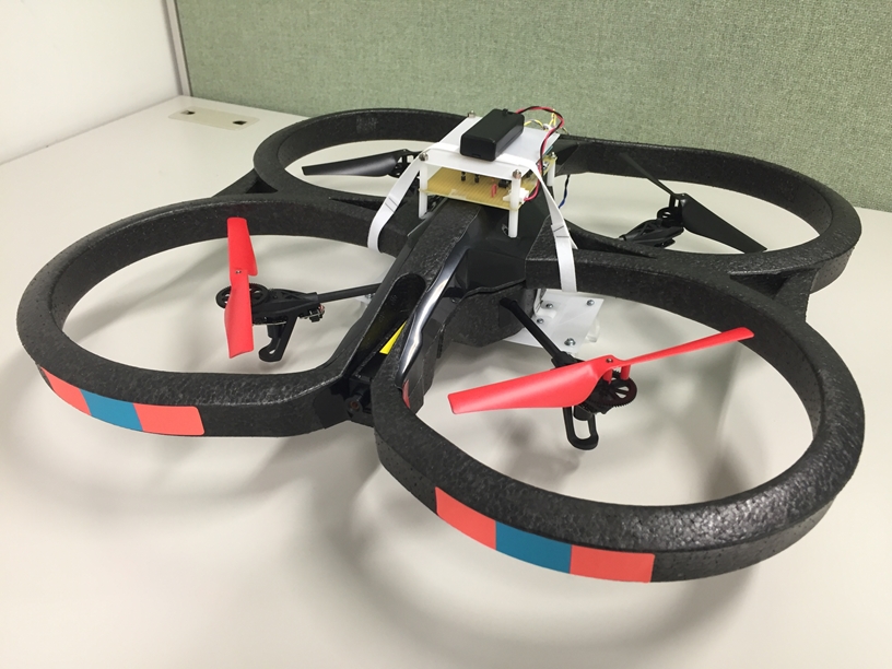
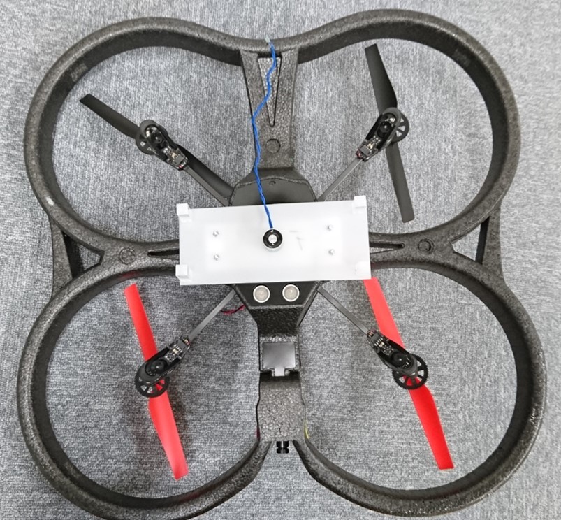
We built a mechanism for attaching/detaching a sensor for the drone. The mechanism consists of an electromagnetic device controlled by a newly developed ROS module. The device can attach/detach a sensor when the electromagnetic power is turned on/off. The maximum load is approximately 50 g, under conditions in which the drone can fly stably. In this study, we assume that the sensor is light-weight (50 g or less) and has a metal part that can be attached to the drone by electromagnetic force. We also assume that each sensor is manually attached to the drone individually, which means that the sensors are not autonomously loaded. Although we assume that the drone can carry one sensor at a time, the method is not limited to this number of sensors.
To make the experimental results reproducible, a simulation environment shown in Figure4 was used in this study. For this purpose, the above hardware was modeled as a simulated robot. We used Gazebo for the simulator and ROS for controlling the drone in the experiments.
VI-B Experimental Settings
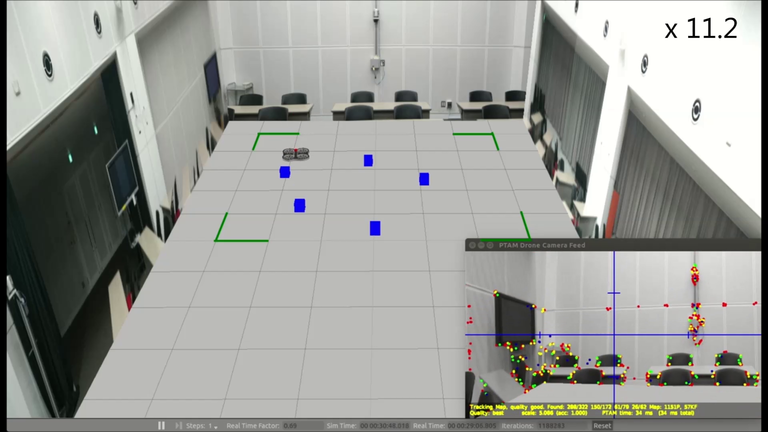
Experiments were conducted in the simulation environment shown in Figure4. In the figure, the blue cubes represent the deployed sensors. In the environment, we set 25 grid points as the target candidates, . The 25 grid points were equally positioned within the 55 m area surrounded by the green lines. Note that even if a sensor was dropped inside the area, it might land outside of it because of deviation.
VI-C Qualitative Results
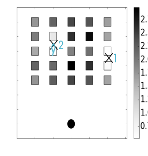
(a) Baseline (2 sensors)
(b) Proposed (2 sensors)
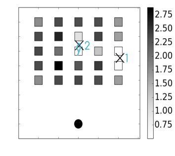
(c) Baseline (5 sensors)
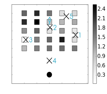
(d) Proposed (5 sensors)
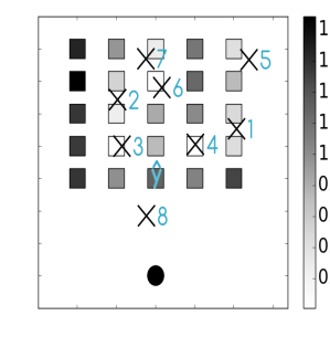
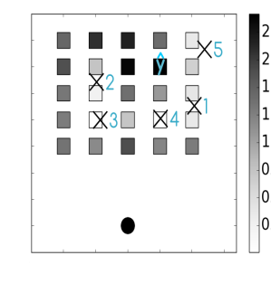
(e) Baseline (8 sensors)
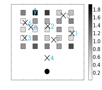
(f) Proposed (8 sensors)
We compared our proposed method (SuMo-SS) and a baseline method. We used the method proposed by Krause[4] as the baseline. Unlike SuMo-SS, the baseline method does not consider the uncertainty of sensor positions.
Figure5 shows the qualitative results, where are set to . The subfigures in the left and right columns are the results of the baseline and SuMo-SS, respectively. The color strength represents (increase in mutual information when sensor is added) after three conditions: (a) and (b) show two sensors, (c) and (d) show five sensors, and (e) and (f) show eight sensors. In the subfigures, the squares, cross marks (“✕”), and black circles represent (set of target position candidates), (actual position of sensor ), and the loading position, respectively. Note that was unobservable from the methods. Numbers in blue represents the ordering of . In each subfigure, ’’ in blue represents each penultimate target position .
The difference in the sensor positions in subfigures (a) and (b) is thought to be caused by deviation, and this indicates that SuMo-SS and the baseline have no significant difference when two sensors are scattered. Although there is a difference between subfigures (c) and (d), the bias in the sensor positions is not significant. By contrast, subfigure (e) shows that the sensors are scattered in a biased manner compared with subfigure (f). This indicates that SuMo-SS could plan to scatter sensors unbiasedly under uncertainty. Because this needs to be quantitatively validated, we show the quantitative validation in Figure6.
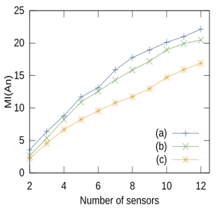
VI-D Quantitative Results
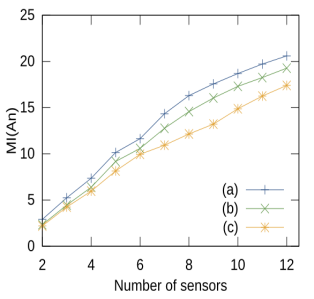
A quantitative comparison is shown in Figure6. The horizontal axis represents the number of sensors, . The vertical axis represents , which is the mutual information when sensors are introduced to the environment. is defined as follows:
| (12) |
where denotes the information gain when the -th sensor is introduced. To satisfy the condition that is a monotonic submodular function, needs to be less than . SuMo-SS and the baseline method require at least one sensor in the environment. Therefore, the first target position was manually given as the center of the area. Then, the second to -th target positions were planned by the proposed and baseline methods.
Figure6 compares the results from (a) SuMo-SS (proposed), (b) baseline[4], and (c) random selection. The random selection method was introduced as the lower bound method, which selected the next target position randomly from . The left-hand and right-hand figures show the results where and , respectively. The average results of 10 experimental runs are shown.
From the left-hand figure of Figure6, SuMo-SS obtained larger than the baseline method. values at obtained by (a) SuMo-SS (proposed), (b) baseline[4], and (c) random selection were 22.14, 20.47, and 16.89, respectively. In the right-hand figure, at obtained by (a), (b), and (c), were 20.59, 19.26, and 17.40, respectively. The above results show that our method obtained better results in both settings.
VI-E Sensitivity Analysis
To validate SuMo-SS under various deviations, we evaluated the performance under various combinations of . The conditions for and were and , respectively. We ran 10 simulations for each combination of . The evaluation was conducted for SuMo-SS and the baseline[4]. Therefore, we ran the simulation 980 () times in total.
TABLEII shows a performance difference between SuMo-SS and the baseline. The performance difference is defined as follows:
| (13) |
where represents the number of sensors. A positive indicates that SuMo-SS obtained larger than the baseline. The subtables (a), (b), (c), and (d) show , , , and , respectively. In each sub-table, the top and bottom three results are displayed in red and blue, respectively.
Sub-table (a) shows that SuMo-SS outperformed the baseline in all conditions (49 out of 49) when the number of introduced sensors was three (). Sub-tables (b), (c) and (d) show that SuMo-SS outperformed the baseline in 41, 46, and 44 conditions when , , and , respectively. These results indicate that SuMo-SS could obtain larger under most of the conditions.
(a)
0.2
0.25
0.3
0.35
0.4
0.45
0.5
0.2
1.05
1.05
0.76
0.68
0.73
0.77
0.44
0.25
1.14
1.09
0.88
0.81
0.99
0.89
0.52
0.3
1.01
0.59
0.72
0.90
1.25
1.20
1.16
0.35
0.95
0.32
0.37
0.79
1.01
0.99
0.83
0.4
1.03
0.54
0.61
0.79
0.94
0.88
0.69
0.45
0.67
0.34
0.63
0.69
0.82
0.74
0.57
0.5
0.18
0.24
0.45
0.51
0.83
0.73
0.57
(b)
0.2
0.25
0.3
0.35
0.4
0.45
0.5
0.2
0.96
0.09
0.92
1.35
1.34
1.22
0.57
0.25
0.84
0.66
0.95
0.86
0.85
1.03
0.44
0.3
0.55
-0.21
0.59
0.65
0.66
0.25
0.83
0.35
0.45
-0.15
0.77
1.05
0.80
0.77
0.68
0.4
0.46
0.05
1.02
0.85
0.94
0.94
1.13
0.45
-0.39
-0.21
0.72
0.32
0.73
0.55
0.64
0.5
-0.82
-1.17
-0.16
-0.42
0.22
0.03
0.32
(c)
0.2
0.25
0.3
0.35
0.4
0.45
0.5
0.2
0.73
-0.28
0.29
1.86
0.80
1.54
0.37
0.25
0.76
0.23
1.34
1.99
0.73
1.46
0.22
0.3
1.73
-0.11
1.31
2.08
1.08
0.45
1.43
0.35
1.96
-0.12
1.46
1.52
1.00
0.30
0.51
0.4
2.06
0.03
2.32
1.50
0.72
0.68
1.06
0.45
1.03
0.08
0.89
0.55
0.81
0.60
1.26
0.5
0.29
0.16
0.30
0.47
0.12
0.27
0.69
(d)
0.2
0.25
0.3
0.35
0.4
0.45
0.5
0.2
0.05
-0.68
0.31
1.67
0.58
0.90
0.10
0.25
0.81
0.22
0.55
1.27
0.43
0.45
-0.48
0.3
1.68
-0.84
1.55
1.61
1.50
0.29
1.59
0.35
1.96
-0.87
2.00
1.33
1.59
0.35
1.00
0.4
1.55
-0.05
2.94
1.41
0.73
0.68
1.19
0.45
0.73
0.15
1.58
0.70
1.10
0.51
1.45
0.5
0.13
-0.06
0.41
0.13
0.34
0.15
0.78
VI-F Discussions
First, we discuss the covariance of the sensor observations. In this study, covariance was obtained based on the sensor positions. This does not mean that SuMo-SS requires precise sensor position information. Instead, this was because (a) our focus is not to model realistic sensor observations, and (b) simulations require a certain-level of approximation on sensor observation. However, this does not hold in real-world applications; therefore, covariance should be calculated based on sensor observations. By doing so, we will be able to apply the proposed method to real-world applications including cases in which scattered sensors are washed away by rain.
We used mutual information as the criterion for submodular optimization. However, we can use other criteria that have submodularity, such as the monitoring area size and the number of grid points covered by the area. Future study includes the improvement of the optimization policy instead of the greedy method. Golovin et al. proposed adaptive policies by introducing the concept of adaptive submodularity[18]. Although the assumptions for submodularity and adaptive submodularity are different, there is a possibility that the SS problem can be extended to satisfy the assumptions.
Figure6 might give the impression that the performance of the baseline and SuMo-SS slightly decrease at . This is caused by the fact that the increase in is decreasing in monotonic submodular functions. In this study, the maximum number of sensors was 12, which is the greatest integer less than . However, this does not mean that the method is limited to 12 sensors. By increasing , more sensors can be deployed without any fundamental changes. For example, if a developer needs to deploy 100 sensors in a practical use case, then can be set because is arbitrary in SuMo-SS.
One might question whether sensors should be simply dropped at grid points; however, not all sensors might be informative because sometimes local events cannot be monitored by rough granularity. Although the sensor material can be changed to reduce the deviation, reducing it to zero will not be easy. Although we used a drone to transport sensors, SuMo-SS can be applied to a setting in which sensors are deployed with catapult-like devices provided that the deviation can be modeled.
VII Summary
In this paper, we made the following contribution:
-
•
We proposed the SuMo-SS method that can deal with uncertainty in sensor positions. Unlike existing methods, SuMo-SS can deal with uncertainty in sensor positions, which is relevant for practical applications. Its experimental validation with a baseline method was explained in Section VI.
The target use case of our method include building sensor networks for environmental monitoring. Future work includes an experimental validation with physical drones in outdoor environments.
Appendix A Appendix
A-A Submodurality in Expected Mutual Information
A set function is called submodular if it holds for every with and every . is proved to be a monotone submodular function in particular conditions[25, 4].
If the probabilistic distribution of is discrete, Equation (7) can be rewritten as follows:
| (14) |
where denotes the probabilistic distribution of . A nonnegative linear combination of submodular functions is also submodular[17, 26]. Therefore, the right-hand term in Equation (14) is submodular. If is continuous instead, we can approximate it with the average of sufficiently fine discrete distributions as shown in Equation (14). Therefore, the expected mutual information shown in Equation (7) is a submodular function.
A-B Submodular Optimization Using Mutual Information
Hereinafter, we explain the method proposed in [4]. For readability, and are written as and , respectively.
From the definition of mutual information, is decomposed as follows:
where represents entropy.
Let be the difference between and as follows:
| (15) |
From the definition of conditional entropy, can be written:
| (16) |
We can also transform in the same manner. Thus Equation (15) can be rewritten:
| (17) |
Another definition of conditional entropy is given as follows:
| (18) |
where the formula of the integral of Gaussian distributions is used. Similarly, we can obtain . From Equations (17) and (18), we obtain
| (19) |
When a multi-variate Gaussian distribution is divided, the following holds:
| (20) |
ACKNOWLEDGMENT
This work was partially supported by JST CREST and JSPS KAKENHI Grant Number JP15K16074.
References
- [1] M. Abdulaal, M. Algarni, A. Shamim, and C. Claudel, “Unmanned Aerial Vehicle Based Flash Flood Monitoring Using Lagrangian Trackers,” International Workshop on Robotic Sensor Networks, 2014.
- [2] A. Krause and C. Guestrin, “Submodularity and Its Applications in Optimized Information Gathering,” ACM Transactions on Intelligent Systems and Technology, vol. 2, no. 4, p. 32, 2011.
- [3] M. Younis and K. Akkaya, “Strategies and techniques for node placement in wireless sensor networks: A survey,” Ad Hoc Networks, vol. 6, no. 4, pp. 621–655, 2008.
- [4] A. Krause, A. Singh, and C. Guestrin, “Near-Optimal Sensor Placements in Gaussian Processes: Theory, Efficient Algorithms and Empirical Studies,” The Journal of Machine Learning Research, vol. 9, pp. 235–284, 2008.
- [5] B. Wang, “Coverage Problems in Sensor Networks: A Survey,” ACM Computing Surveys, vol. 43, no. 4, p. 32, 2011.
- [6] W. E. Hart and R. Murray, “Review of Sensor Placement Strategies for Contamination Warning Systems in Drinking Water Distribution Systems,” Journal of Water Resources Planning and Management, vol. 136, no. 6, pp. 611–619, 2010.
- [7] P. Corke, S. Hrabar, R. Peterson, D. Rus, S. Saripalli, and G. Sukhatme, “Autonomous Deployment and Repair of a Sensor Network Using an Unmanned Aerial Vehicle,” in Proc. IEEE ICRA, vol. 4, 2004, pp. 3602–3608.
- [8] J. Valente, D. Sanz, A. Barrientos, J. d. Cerro, Á. Ribeiro, and C. Rossi, “An Air-Ground Wireless Sensor Network for Crop Monitoring,” Sensors, vol. 11, no. 6, pp. 6088–6108, 2011.
- [9] H. Huang, “Performance Improvement by Introducing Mobility in Wireless Communication Networks,” arXiv:1712.02436, 2017.
- [10] M. Alzenad, A. El-Keyi, F. Lagum, and H. Yanikomeroglu, “3-D Placement of an Unmanned Aerial Vehicle Base Station (UAV-BS) for Energy-Efficient Maximal Coverage,” IEEE Wireless Communications Letters, vol. 6, no. 4, pp. 434–437, 2017.
- [11] S. Thrun, W. Burgard, and D. Fox, Probabilistic Robotics. MIT Press, 2005.
- [12] C. Stachniss, G. Grisetti, and W. Burgard, “Information Gain-based Exploration Using Rao-Blackwellized Particle Filters,” in Robotics: Science and Systems, vol. 2, 2005, pp. 65–72.
- [13] R. Sim and N. Roy, “Global a-optimal robot exploration in slam,” in Proc. IEEE ICRA, 2005, pp. 661–666.
- [14] P. P. Neumann, V. Hernandez Bennetts, A. J. Lilienthal, M. Bartholmai, and J. H. Schiller, “Gas Source Localization with a Micro-drone Using Bio-inspired and Particle Filter-based Algorithms,” Advanced Robotics, vol. 27, no. 9, pp. 725–738, 2013.
- [15] C. Chekuri and M. Pal, “A Recursive Greedy Algorithm for Walks in Directed Graphs,” in Proc. 46th Annual IEEE Symposium on Foundations of Computer Science, 2005, pp. 245–253.
- [16] A. Singh, A. Krause, C. Guestrin, and W. J. Kaiser, “Efficient Informative Sensing Using Multiple Robots,” Journal of Artificial Intelligence Research, vol. 34, pp. 707–755, 2009.
- [17] A. Krause, J. Leskovec, C. Guestrin, J. VanBriesen, and C. Faloutsos, “Efficient Sensor Placement Optimization for Securing Large Water Distribution Networks,” Journal of Water Resources Planning and Management, vol. 134, no. 6, pp. 516–526, 2008.
- [18] D. Golovin and A. Krause, “Adaptive Submodularity: Theory and Applications in Active Learning and Stochastic Optimization,” Journal of Artificial Intelligence Research, vol. 42, pp. 427–486, 2011.
- [19] R. K. Williams, A. Gasparri, and G. Ulivi, “Decentralized Matroid Optimization for Topology Constraints in Multi-Robot Allocation Problems,” in Proc. IEEE ICRA, 2017, pp. 293–300.
- [20] S. Chen, Y. Li, and N. M. Kwok, “Active Vision in Robotic Systems: A Survey of Recent Developments,” International Journal of Robotics Research, vol. 30, no. 11, pp. 1343–1377, 2011.
- [21] V. Akbarzadeh, C. Gagné, M. Parizeau, M. Argany, and M. A. Mostafavi, “Probabilistic Sensing Model for Sensor Placement Optimization Based on Line-of-Sight Coverage,” IEEE Trans. Instrumentation and Measurement, vol. 62, no. 2, pp. 293–303, 2013.
- [22] K. Washizaki, M. Wakabayashi, and M. Kumon, “Position Estimation of Sound Source on Ground by Multirotor Helicopter with Microphone Array,” in Proc. IEEE/RSJ IROS, 2016, pp. 1980–1985.
- [23] K. Nakadai, M. Kumon, H. G. Okuno, K. Hoshiba, M. Wakabayashi, K. Washizaki, T. Ishiki, D. Gabriel, Y. Bando, T. Morito, et al., “Development of Microphone-Array-Embedded UAV for Search and Rescue Task,” in Proc. IEEE/RSJ IROS, 2017, pp. 5985–5990.
- [24] J. Engel, J. Sturm, and D. Cremers, “Scale-Aware Navigation of a Low-Cost Quadrocopter with a Monocular Camera,” Robotics and Autonomous Systems, vol. 62, no. 11, pp. 1646–1656, 2014.
- [25] G. L. Nemhauser, L. A. Wolsey, and M. L. Fisher, “An Analysis of Approximations for Maximizing Submodular Set Functions,” Mathematical Programming, vol. 14, no. 1, pp. 265–294, 1978.
- [26] D. Kempe, J. Kleinberg, and É. Tardos, “Maximizing the Spread of Influence through a Social Network,” in Proc. of ACM SIGKDD, 2003, pp. 137–146.