iFair: Learning Individually Fair Data Representations for Algorithmic Decision Making

Abstract

People are rated and ranked, towards algorithmic decision making in an increasing number of applications, typically based on machine learning. Research on how to incorporate fairness into such tasks has prevalently pursued the paradigm of group fairness: giving adequate success rates to specifically protected groups. In contrast, the alternative paradigm of individual fairness has received relatively little attention, and this paper advances this less explored direction. The paper introduces a method for probabilistically mapping user records into a low-rank representation that reconciles individual fairness and the utility of classifiers and rankings in downstream applications. Our notion of individual fairness requires that users who are similar in all task-relevant attributes such as job qualification, and disregarding all potentially discriminating attributes such as gender, should have similar outcomes. We demonstrate the versatility of our method by applying it to classification and learning-to-rank tasks on a variety of real-world datasets. Our experiments show substantial improvements over the best prior work for this setting.

This is a preprint of a full paper at ICDE 2019. Please cite the ICDE proceedings version.

I Introduction

Motivation: People are rated, ranked and selected or not selected in an increasing number of online applications, towards algorithmic decisions based on machine learning models. Examples are approvals or denials of loans or visas, predicting recidivism for law enforcement, or rankings in job portals. As algorithmic decision making becomes pervasive in all aspects of our daily life, societal and ethical concerns [1, 6] are rapidly growing. A basic approach is to establish policies that disallow the inclusion of potentially discriminating attributes such as gender or race, and ensure that classifiers and rankings operate solely on task-relevant attributes such as job qualifications.

The problem has garnered significant attention in the data-mining and machine-learning communities. Most of this work considers so-called group fairness models, most notably, the statistical parity of outcomes in binary classification tasks, as a notion of fairness. Typically, classifiers are extended to incorporate demographic groups in their loss functions, or include constraints on the fractions of groups in the accepted class [3, 17, 18, 23, 10, 11] to reflect legal boundary conditions and regulatory policies. For example, computing a shortlist of people invited for job interviews should have a gender mix that is proportional to the base population of job applicants.

The classifier objective is faced with a fundamental trade-off between utility (typically accuracy) and fairness, and needs to aim for a good compromise. Other definitions of group fairness have been proposed [15, 26, 29], and variants of group fairness have been applied to learning-to-rank tasks [27, 25, 24]. In all these cases, fair classifiers or regression models need an explicit specification of sensitive attributes such as gender, and often the identification of a specific protected (attribute-value) group such as gender equals female.

The Case for Individual Fairness: Dwork et al. [8] argued that group fairness, while appropriate for policies regarding demographic groups, does not capture the goal of treating individual people in a fair manner. This led to the definition of individual fairness: similar individuals should be treated similarly. For binary classifiers, this means that individuals who are similar on the task-relevant attributes (e.g., job qualifications) should have nearly the same probability of being accepted by the classifier. This kind of fairness is intuitive and captures aspects that group fairness does not handle. Most importantly, it addresses potential discrimination of people by disparate treatment despite the same or similar qualifications (e.g., for loan requests, visa applications or job offers), and it can mitigate such risks.

Problem Statement: Unfortunately, the rationale for capturing individual fairness has not received much follow-up work – the most notable exception being [28] as discussed below. The current paper advances the approach of individual fairness in its practical viability, and specifically addresses the key problem of coping with the critical trade-off between fairness and utility: How can a data-driven system provide a high degree of individual fairness while also keeping the utility of classifiers and rankings high? Is this possible in an application-agnostic manner, so that arbitrary downstream applications are supported? Can the system handle situations where sensitive attributes are not explicitly specified at all or become known only at decision-making time (i.e., after the system was trained and deployed)?

Simple approaches like removing all sensitive attributes from the data and then performing a standard clustering technique do not reconcile these two conflicting goals, as standard clustering may lose too much utility and individual fairness needs to consider attribute correlations beyond merely masking the explicitly protected ones. Moreover, the additional goal of generality, in terms of supporting arbitrary downstream applications, mandates that cases without explicitly sensitive attributes or with sensitive attributes being known only at decision-making time be gracefully handled as well.

The following example illustrates the points that a) individual fairness addresses situations that group fairness does not properly handle, and b) individual fairness must be carefully traded off against the utility of classifiers and rankings.

Example: Table I shows a real-world example for the issue of unfairness to individual people. Consider the ranked results for an employer’s query “Brand Strategist” on the German job portal Xing; that data was originally used in Zehlike et al. [27]. The top-10 results satisfy group fairness with regard to gender, as defined by Zehlike et al. [27] where a top-k ranking $\tau$ is fair if for every prefix $\tau|i=<\tau(1),\tau(2),\cdots\tau(i)>$ ($1\leq i\leq k$) the set $\tau|i$ satisfies statistical parity with statistical significance $\alpha$. However the outcomes in Table I are far from being fair for the individual users: people with very similar qualifications, such as Work Experience and Education Score ended up on ranks that are far apart (e.g., ranks 5 and 30). By the position bias [16] when searchers browse result lists, this treats the low-ranked people quite unfairly. This demonstrates that applications can satisfy group-fairness policies, while still being unfair to individuals.

Search Query	Work	Education	Candidate	Xing
	Experience	Experience		Ranking
Brand Strategist	146	57	male	1
Brand Strategist	327	0	female	2
Brand Strategist	502	74	male	3
Brand Strategist	444	56	female	4
Brand Strategist	139	25	male	5
Brand Strategist	110	65	female	6
Brand Strategist	12	73	male	7
Brand Strategist	99	41	male	8
Brand Strategist	42	51	female	9
Brand Strategist	220	102	female	10
		$\cdots$
Brand Strategist	3	107	female	20
Brand Strategist	123	56	female	30
Brand Strategist	3	3	male	40

TABLE I: Top k results on www.xing.com (Jan 2017) for an employer’s job search query “Brand Strategist”.

State of the Art and its Limitations: Prior work on fairness for ranking tasks has exclusively focused on group fairness [27, 25, 24], disregarding the dimension of individual fairness. For the restricted setting of binary classifiers, the most notable work on individual fairness is [28]. That work addresses the fundamental trade-off between utility and fairness by defining a combined loss function to learn a low-rank data representation. The loss function reflects a weighed sum of classifier accuracy, statistical parity for a single pre-specified protected group, and individual fairness in terms of reconstruction loss of data. This model, called LFR, is powerful and elegant, but has major limitations:

• It is geared for binary classifiers and does not generalize to a wider class of machine-learning tasks, dismissing regression models, i.e., learning-to-rank tasks.

• Its data representation is tied to a specific use case with a single protected group that needs to be specified upfront. Once learned, the representation cannot be dynamically adjusted to different settings later.

• Its objective function strives for a compromise over three components: application utility (i.e., classifier accuracy), group fairness and individual fairness. This tends to burden the learning with too many aspects that cannot be reconciled.

Our approach overcomes these limitations by developing a model for representation learning that focuses on individual fairness and offers greater flexibility and versatility.

Approach and Contribution: The approach that we put forward in this paper, called iFair, is to learn a generalized data representation that preserves the fairness-aware similarity between individual records while also aiming to minimize or bound the data loss. This way, we aim to reconcile individual fairness and application utility, and we intentionally disregard group fairness as an explicit criterion.

iFair resembles the model of [28] in that we also learn a representation via probabilistic clustering, using a form of gradient descent for optimization. However, our approach differs from [28] on a number of major aspects:

• iFair learns flexible and versatile representations, instead of committing to a specific downstream application like binary classifiers. This way, we open up applicability to arbitrary classifiers and support regression tasks (e.g., rating and ranking people) as well.

• iFair does not depend on a pre-specified protected group. Instead, it supports multiple sensitive attributes where the “protected values” are known only at run-time after the application is deployed. For example, we can easily handle situations where the critical value for gender is female for some ranking queries and male for others.

• iFair does not consider any notion of group fairness in its objective function. This design choice relaxes the optimization problem, and we achieve much better utility with very good fairness in both classification and ranking tasks. Hard group-fairness constraints, based on legal requirements, can be enforced post-hoc by adjusting the outputs of iFair-based classifiers or rankings.

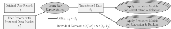
Figure 1: Overview of decision-making pipeline.

The novel contributions of iFair are: 1) the first method, to the best of our knowledge, that provides individual fairness for learning-to-rank tasks; 2) an application-agnostic framework for learning low-rank data representations that reconcile individual fairness and utility such that application-specific choices on sensitive attributes and values do not require learning another representation; 3) experimental studies with classification and regression tasks for downstream applications, empirically showing that iFair can indeed reconcile strong individual fairness with high utility. The overall decision-making pipeline is illustrated in Figure 1.

II Related work

Fairness Definitions and Measures: Much of the work in algorithmic fairness has focused on supervised machine learning, specifically on the case of binary classification tasks. Several notions of group fairness have been proposed in the literature. The most widely used criterion is statistical parity and its variants [3, 17, 18, 23, 10, 11]. Statistical parity states that the predictions $\hat{Y}$ of a classifier are fair if members of sensitive subgroups, such as people of certain nationalities or ethnic backgrounds, have an acceptance likelihood proportional to their share in the entire data population. This is equivalent to requiring that apriori knowledge of the classification outcome of an individual should provide no information about her membership to such subgroups. However, for many applications, such as risk assessment for credit worthiness, statistical parity is neither feasible nor desirable.

Alternative notions of group fairness have been defined. Hardt et al. [15] proposed equal odds which requires that the rates of true positives and false positives be the same across groups. This punishes classifiers which perform well only on specific groups. Hardt et al. [15] also proposed a relaxed version of equal odds called equal opportunity which demands only the equality of true positive rates. Other definitions of group fairness include calibration [12, 19], disparate mistreatment [26], and counterfactual fairness [20]. Recent work highlights the inherent incompatibility between several notions of group fairness and the impossibility of achieving them simultaneously [19, 4, 13, 5].

Dwork et al. [8] gave the first definition of individual fairness, arguing for the fairness of outcomes for individuals and not merely as a group statistic. Individual fairness mandates that similar individuals should be treated similarly. [8] further develops a theoretical framework for mapping individuals to a probability distribution over outcomes, which satisfies the Lipschitz property (i.e., distance preservation) in the mapping. In this paper, we follow up on this definition of individual fairness and present a generalized framework for learning individually fair representations of the data.

Fairness in Machine Learning: A parallel line of work in the area of algorithmic fairness uses a specific definition of fairness in order to design fairness models that achieve fair outcomes. To this end, there are two general strategies. The first strategy consists of de-biasing the input data by appropriate preprocessing [17, 23, 10]. This typically involves data perturbation such as modifying the value of sensitive attributes or class labels in the training data to satisfy certain fairness conditions, such as equal proportion of positive (negative) class labels in both protected and non-protected groups . The second strategy consists of designing fair algorithmic models - based on constrained optimization [3, 18, 15, 26]. Here, fairness constraints are usually introduced as regularization terms in the objective function.

Fairness in IR: Recently, definitions of group fairness have been extended to learning-to-rank tasks. Yang and Stoyanovich [25] introduced statistical parity in rankings. Zehlike et al. [27] built on [25] and proposed to ensure statistical parity at all top-k prefixes of the ranked results. Singh and Joachims [24] proposed a generalized fairness framework for a larger class of group fairness definitions (e.g., disparate treatment and disparate impact). However, all this prior work has focused on group fairness alone. It implicitly assumes that individual fairness is taken care of by the ranking quality, disregarding situations where trade-offs arise between these two dimensions. The recent work of Biega et al. [2] addresses individual fairness in rankings from the perspective of giving fair exposure to items over a series of rankings, thus mitigating the position bias in click probabilities. In their approach they explicitly assume to have access to scores that are already individually fair. As such, their work is complementary to ours as they do not address how such a score, which is individually fair can be computed.

Representation Learning: The work of Zemel et al. [28] is the closest to ours in that it is also learns low-rank representations by probabilistic mapping of data records. However, the methods deviates from our in important ways. First, its fair representations are tied to a particular classifier by assuming a binary classification problem with pre-specified labeling target attribute and a single protected group. In contrast, the representations learned by iFair are agnostic to the downstream learning tasks and thus easily deployable for new applications. Second, the optimization in [28] aims to combine three competing objectives: classifier accuracy, statistical parity, and data loss (as a proxy for individual fairness). The iFair approach, on the other hand, addresses a more streamlined objective function by focusing on classifier accuracy and individual fairness.

Approaches similar to [28] have been applied to learn censored representations for fair classifiers via adversarial training [22, 9]. Group fairness criteria are optimized in the presence of an adversary. These approaches do not consider individual fairness at all.

III Model

We consider user records that are fed into a learning algorithm towards algorithm decision making. A fair algorithm should make its decisions solely based on non-sensitive attributes (e.g., technical qualification or education) and should disregard sensitive attributes that bear the risk of discriminating users (e.g., ethnicity/race). This dichotomy of attributes is specified upfront, by domain experts and follows legal regulations and policies. Ideally, one should consider also strong correlations (e.g., geo-area correlated with ethnicity/race), but this is usually beyond the scope of the specification. We start with introducing preliminary notations and definitions.

Input Data: The input data for $M$ users with $N$ attributes is an $M\times N$ matrix $X$ with binary or numerical values (i.e., after unfolding or encoding categorical attributes). Without loss of generality, we assume that the attributes $1~{}..~{}l$ are non-protected and the attributes $l+1~{}..~{}N$ are protected. We denote the $i$-th user record consisting of all attributes as $x_{i}$ and only non-protected attributes as $x_{i}^{\ast}$. Note that, unlike in prior works, the set of protected attributes is allowed to be empty (i.e., $l=N$). Also, we do not assume any upfront specification of which attribute values form a protected group. So a downstream application can flexibly decide on the critical values (e.g., male vs. female or certain choices of citizenships) on a case-by-case basis.

Output Data: The goal is to transform the input records $x_{i}$ into representations $\tilde{x_{i}}$ that are directly usable by downstream applications and have better properties regarding fairness. Analogously to the input data, we can write the entire output of $\tilde{x_{i}}$ records as an $M\times N$ matrix $\tilde{X}$.

Individually Fair Representation: Inspired by the Dwork et al. [8] notion of individual fairness, “individuals who are similar should be treated similarly”, we propose the following definition for individual fairness:

Definition 1. (Individual Fairness) Given a distance function $d$ in the $N-$dimensional data space, a mapping $\phi$ of input records $x_{i}$ into output records $\tilde{x_{i}}$ is individually fair if for every pair $x_{i},x_{j}$ we have

$$\lvert d(\phi(x_{i}),\phi(x_{j}))-d(x_{i}^{*},x_{j}^{*})\rvert\leq\epsilon$$ (1)

The definition requires that individuals who are (nearly) indistinguishable on their non-sensitive attributes in $X$ should also be (nearly) indistinguishable in their transformed representations $\tilde{X}$. For example, two people with (almost) the same technical qualifications for a certain job should have (almost) the same low-rank representation, regardless of whether they differ on protected attributes such as gender, religion or ethnic group. In more technical terms, a distance measure between user records should be preserved in the transformed space.

Note that this definition intentionally deviates from the original definition of individual fairness of [8] in that with $x_{i}^{*},x_{j}^{*}$ we consider only the non-protected attributes of the original user records, as protected attributes should not play a role in the decision outcomes of an individual.

III-A Problem Formulation: Probabilistic Clustering

As individual fairness needs to preserve similarities between records $x_{i},x_{j}$, we cast the goal of computing good representations $\tilde{x_{i}},\tilde{x_{j}}$ into a formal problem of probabilistic clustering. We aim for $K$ clusters, each given in the form of a prototype vector $v_{k}$ ($k=1..K$), such that records $x_{i}$ are assigned to clusters by a record-specific probability distribution that reflects the distances of records from prototypes. This can be viewed as a low-rank representation of the input matrix $X$ with $K<M$, so that we reduce attribute values into a more compact form. As always with soft clustering, $K$ is a hyper-parameter.

Definition 2. (Transformed Representation) The fair representation $\tilde{X}$, an $M\times N$ matrix of row-vise output vectors $\tilde{x_{i}}$, consists of

• $K<M$ prototype vectors $v_{k}$, each of dimensionality $N$,

• a probability distribution $u_{i}$, of dimensionality $K$, for each input record $x_{i}$ where $u_{ik}$ is the probability of $x_{i}$ belonging to the cluster of prototype $v_{k}$.

The representation $\tilde{x_{i}}$ is given by

$$\tilde{x_{i}}=\sum_{k=1..K}u_{ik}\cdot v_{k}\vspace{2mm}$$ (2)

or equivalently in matrix form: $\tilde{X}=U\times V^{T}$ where the rows of $U$ are the per-record probability distributions and the columns of $V^{T}$ are the prototype vectors.

Definition 3. (Transformation Mapping) We denote the mapping $x_{i}\rightarrow\tilde{x_{i}}$ as $\phi$; that is,

$$\phi(x_{i})=\tilde{x_{i}}=\sum_{k=1..K}u_{ik}\cdot v_{k}$$ (3)

using Equation 2.

Utility Objective: Without making any assumptions on the downstream application, the best way of ensuring high utility is to minimize the data loss induced by $\phi$. Definition 4. (Data Loss) The reconstruction loss between $X$ and $\tilde{X}$ is the sum of squared errors

$$L_{util}(X,\tilde{X})=\sum\limits_{i=1}^{M}||x_{i}-\tilde{x}_{i}||_{2}=\sum\limits_{i=1}^{M}\sum\limits_{j=1}^{N}(x_{ij}-\tilde{x}_{ij})^{2}$$ (4)

Individual Fairness Objective: Following the rationale for Definition 1, the desired transformation $\phi$ should preserve pair-wise distances between data records on non-protected attributes.

Definition 5. (Fairness Loss) For input data $X$, with row-wise data records $x_{i}$, and its transformed representation $\tilde{X}$ with row-wise $\tilde{x_{i}}$, the fairness loss $L_{fair}$ is

$$L_{fair}(X,\tilde{X})=\sum_{i,j=1..M}\left(d(\tilde{x_{i}},\tilde{x_{j}})-d(x^{*}_{i},x^{*}_{j})\right)^{2}$$ (5)

Overall Objective Function: Combing the data loss and the fairness loss yields our final objective function that the learned representain should aim to minimize.

Definition 6. (Objective Function) The combined objective function is given by

$$L=\lambda\cdot L_{util}(X,\tilde{X})+\mu\cdot L_{fair}(X,\tilde{X})$$ (6)

where $\lambda$ and $\mu$ are hyper-parameters.

III-B Probabilistic Prototype Learning

So far we have left the choice of the distance function $d$ open. Our methodology is general and can incorporate a wide suite of distance measures. However, for the actual optimization, we need to make a specific choice for $d$. In this paper, we focus on the family of Minkowski p-metrics, which is indeed a metric for $p\geq 1$. A common choice is $p=2$, which corresponds to a Gaussian kernel.

Definition 7. (Distance Function) The distance between two data records $x_{i},x_{j}$ is

$$d(x_{i},x_{j})=\big{[}\sum\limits_{n=1}^{N}\alpha_{n}(x_{i,n}-x_{j,n})^{p}\big{]}^{1/p}$$ (7)

where $\alpha$ is an $N$-dimensional vector of tunable or learnable weights for the different data attributes.

This distance function $d$ is applicable to original data records $x_{i}$, transformed vectors $\tilde{x_{i}}$ and prototype vectors $v_{k}$ alike. In our model, we avoid the quadratic number of comparisons for all record pairs, and instead consider distances only between records and prototype vectors (cf. also [28]). Then, these distances can be used to define the probability vectors $u_{i}$ that hold the probabilities for record $x_{i}$ belonging to the cluster with prototype $v_{k}$ (for $k=1..K$). To this end, we apply a softmax function to the distances between record and prototype vectors.

Definition 8. (Probability Vector) The probability vector $u_{i}$ for record $x_{i}$ is

$$u_{i,k}=\frac{exp(-d(x_{i},v_{k}))}{\sum\limits_{j=1}^{K}exp(-d(x_{i},v_{j}))}$$ (8)

The mapping $\phi$ that transforms $x_{i}$ into $\tilde{x_{i}}$ can be written as

$$\phi(x_{i})=\sum\limits_{k=1}^{K}\frac{exp(-d(x_{i},v_{k}))}{\sum\limits_{j=1}^{K}exp(-d(x_{i},v_{j}))}\cdot v_{k}$$ (9)

With these definitions in place, the task of learning fair representations $\tilde{x_{i}}$ now amounts to computing $K$ prototype vectors $v_{k}$ and the $N$-dimensional weight vector $\alpha$ in $d$ such that the overall loss function $L$ is minimized.

Definition 9. (Optimization Objective) The optimization objective is to compute $v_{k}$ ($k=1..K$) and $\alpha_{n}$ ($n=1..N$) as argmin for the loss function

$$L =\lambda\cdot L_{util}(X,\tilde{X})~{}~{}+~{}~{}\mu\cdot L_{fair}(X,\tilde{X})$$

$$=\lambda\cdot\sum\limits_{i=1}^{M}\sum\limits_{j=1}^{N}(x_{ij}-\tilde{x}_{ij})^{2}+\mu\cdot\smashoperator[]{\sum_{i,j=1..M}^{}}\left(d(\tilde{x_{i}},\tilde{x_{j}})-d(x^{*}_{i},x^{*}_{j})\right)^{2}$$

where $\tilde{x}_{ij}$ and $d$ are substituted using Equations 9 and 7.

The $N-$dimensional weight vector $\alpha$ controls the influence of each attribute. Given our definition of individual fairness (which intentionally deviates from the original definition in Dwork et al. [8]), a natural setting is to give no weight to the protected attributes as these should not play any role in the similarity of (qualifications of) users. In our experiments, we observe that giving (near-)zero weights to the protected attributes increases the fairness of the learned data representations (see Section V).

III-C Gradient Descent Optimization:

Given this setup, the learning system minimizes the combined objective function given by

$$L=\lambda\cdot L_{util}(X,\tilde{X})+\mu\cdot L_{fair}(X,\tilde{X})\vspace{2mm}$$ (10)

where $L_{util}$ is the data loss, $L_{fair}$ is the loss in individual fairness, and $\lambda$ and $\mu$ are hyper-parameters. We have two sets of model parameters to learn

1. $v_{k}$ ($k=1..K$), the $N-$dimensional prototype vectors,

2. $\alpha$, the $N-$dimensional weight vector of the distance function in Equation 7.

We apply the $L$-$BFGS$ algorithm [21], a quasi-Newton method, to minimize Equation 10 and learn the model parameters.

IV Properties of the iFair Model

We discuss properties of iFair representations and empirically compare iFair to the LFR model. We are interested in the general behavior of methods for learned representations, to what extent they can reconcile utility and individual fairness at all, and how they relate to group fairness criteria (although iFair does not consider these in its optimization). To this end, we generate synthetic data with systematic parameter variation as follows. We restrict ourselves to the case of a binary classifier.

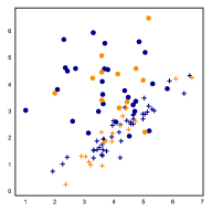
(a) original data (random)

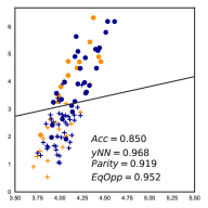
(b) Learned representation via iFair

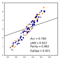
(c) Learned representation via LFR

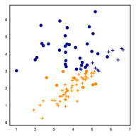
(d) original data ($X1\leq 3$)

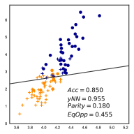
(e) Learned representation via iFair

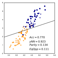
(f) Learned representation via LFR

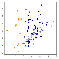
(g) original data ($X2\leq 3$)

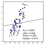
(h) Learned representation via iFair

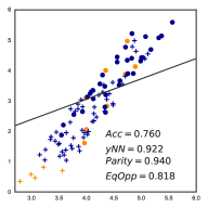
(i) Learned representation via LFR

Figure 2: Illustration of properties of data representations on synthetic data. (left: original data, center: iFair, right: LFR). Output class labels: o for Y=0 and + for Y=1. Membership in protected group: blue for A=0 and orange for A=1. Solid lines are the decision boundaries of the respective classifiers. iFair outperforms LFR on all metrics except for statistical parity.

We generate 100 data points with 3 attributes: 2 real-valued and non-sensitive attributes $X1$ and $X2$ and 1 binary attribute $A$ which serves as the protected attribute. We first draw two-dimensional datapoints from a mixture of Gaussians with two components: (i) isotropic Gaussian with unit variance and (ii) correlated Gaussian with covariance 0.95 between the two attributes and variance 1 for each attribute. To study the influence of membership to the protected group (i.e., $A$ set to 1), we generate three variants of this data:

• Random: $A$ is set to 1 with probability $0.3$ at random.

• Correlation with $X1$: $A$ is set to $1$ if $X1\leq 3$.

• Correlation with $X2$: $A$ is set to $1$ if $X2\leq 3$.

So the three synthetic datasets have the same values for the non-sensitive attributes $X1$ and $X2$ as well for the outcome variable $Y$. The datapoints differ only on membership to the protected group and its distribution across output classes $Y$.

Figure 2 shows these three cases row-wise: subfigures a-c, d-f, g-i, respectively. The left column of the figure displays the original data, with the two labels for output $Y$ depicted by marker: “o” for $Y=0$ and “+” for $Y=1$ and the membership to the protected group by color: orange for $A=1$ and blue for $A=0$. The middle column of Figure 2 shows the learned iFair representations, and the right column shows the representations based on LFR. Note that the values of importance in Figure 2 (middle and right column) are the positions of the data points in the two-dimensional latent space and the classifier decision boundary (solid line). The color of the datapoints and the markers (o and +) depict the true class and true group membership, and not the learned values. They are visualized to aid the reader in relating original data with transformed representations. Furthermore, small differences in the learned representation are expected due to random initializations of model parameters. The solid line in the charts denotes the predicted classifiers’ decision boundary applied on the learned representations. Hyper-parameters for both iFair as well as LFR are chosen by performing a grid search on the set $\{0,0.05,0.1,1,10,100\}$ for optimal individual fairness of the classifier. For each of the nine cases, we indicate the resulting classifier accuracy $Acc$, individual fairness in terms of consistency $yNN$ with regard to the $k=10$ nearest neighbors [28] (formal definition given in Section V-C), the statistical parity $Parity$ with regard to the protected group $A=1$, and equality-of-opportunity $EqOpp$ [15] notion of group fairness.

Main findings: Two major insights from this study are: (i) representations learned via iFair remain nearly the same irrespective of changes in group membership, and (ii) iFair significantly outperforms LFR on accuracy, consistency and equality of opportunity, whereas LFR wins on statistical parity. In the following we further discuss these findings and their implications.

Influence of Protected Group: The middle column in Figure 2 shows that the iFair representation remains largely unaffected by the changes in the group memberships of the datapoints. In other words, changing the value of the protected attribute of a datapoint, all other attribute values remaining the same, has hardly any influence on its learned representation; consequently it has nearly no influence on the outcome made by the decision-making algorithms trained on these representations. This is an important and interesting characteristic to have in a fair representation, as it directly relates to the definition of individual fairness. In contrast, the membership to the protected group has a pronounced influence on the learned representation of the LFR model (refer to Figure 2 right column). Recall that the color of the datapoints as well as the markers (o and +) are taken from the original data. They depict the true class and membership to group of the datapoints, and are visualized to aid the reader.

Tension in Objective Function: The optimization via LFR [28] has three components: classifier accuracy as utility metric, individual fairness in terms of data loss, and group fairness in terms of statistical parity. We observe that by pursuing group fairness and individual fairness together, the tension with utility is very pronounced. The learned representations are stretched on the compromise over all three goals, ultimately leading to sacrificing utility. In contrast, iFair pursues only utility and individual fairness, and disregards group fairness. This helps to make the multi-objective optimization more tractable. iFair clearly outperforms LFR not only on accuracy, with better decision boundaries, but also wins in terms of individual fairness. This shows that the tension between utility and individual fairness is lower than between utility and group fairness.

Trade-off between Utility and Individual Fairness: The improvement that iFair achieves in individual fairness comes at the expense of a small drop in utility. The trade-off is caused by the loss of information in learning representative prototypes. The choice of the mapping function in Equation 9 and the pairwise distance function $d(.)$ in Definition 7 affects the ability to learn prototypes. Our framework is flexible and easily supports other kernels and distance functions. Exploring these influence factors is a direction for future work.

V Experiments

The key hypothesis that we test in the experimental evaluation is whether iFair can indeed reconcile the two goals of individual fairness and utility reasonably well. As iFair is designed as an application-agnostic representation, we test its versatility by studying both classifier and learning-to-rank use cases, in Subsections V-D and V-E, respectively. We compare iFair to a variety of baselines including LFR [28] for classification and FA*IR [27] for ranking. Although group fairness and their underlying legal and political constraints are not among the design goals of our approach, we include group fairness measures in reporting on our experiments – shedding light into this aspect from an empirical perspective.

V-A Datasets

We apply the iFair framework to five real-world, publicly available datasets, previously used in the literature on algorithmic fairness.

• ProPublica’s COMPAS recidivism dataset [1], a widely used test case for fairness in machine learning and algorithmic decision making. We set race as a protected attribute, and use the binary indicator of recidivism as the outcome variable $Y$.

• Census Income dataset consists of survey results of income of 48,842 adults in the US [7]. We use gender as the protected attribute and the binary indicator variable of income $>50K$ as the outcome variable Y.

• German Credit data has $1000$ instances of credit risk assessment records [7]. Following the literature, we set age as the sensitive attribute, and credit worthiness as the outcome variable.

• Airbnb data consists of house listings from five major cities in the US, collected from http://insideairbnb.com/get-the-data.html (June 2018). After appropriate data cleaning, there are $27,597$ records. For experiments, we choose a subset of 22 informative attributes (categorical and numerical) and infer host gender from host name, using lists of common first names. We use gender of the host as the protected attribute and rating/price as the ranking variable.

• Xing is a popular job search portal in Germany (similar to LinkedIn). We use the anonymized data given by [27], consisting of top $40$ profiles returned for $57$ job queries. For each candidate we collect information about job category, work experience, education experience, number of views of the person’s profile, and gender. We set gender as the protected attribute. We use a weighted sum of work experience, education experience and number of profile views as a score that serves as the ranking variable.

The Compas, Census and Credit datasets are used for experiments on classification, and the Xing and Airbnb datasets are used for experiments on learning-to-rank regression. Table II gives details of experimental settings and statistics for each dataset, including base-rate (fraction of samples belonging to the positive class, for both the protected group and its complement), and dimensionality M (after unfolding categorical attributes). We choose the protected attributes and outcome variables to be in line with the literature. In practice, however, such decisions would be made by domain experts and according to official policies and regulations. The flexibility of our framework allows for multiple protected attributes, multivariate outcome variable, as well as inputs of all data types.

Dataset	Base-rate	Base-rate	N	M	Outcome	Protected
	protected	unprotected
Compas	0.52	0.40	6901	431	recidivism	race
Census	0.12	0.31	48842	101	income	gender
Credit	0.67	0.72	1000	67	loan default	age
Airbnb	-	-	27597	33	rating/price	gender
Xing	-	-	2240	59	work + education	gender

TABLE II: Experimental settings and statistics of the datasets.

V-B Setup and Baselines

In each dataset, categorical attributes are transformed using one-hot encoding, and all features vectors are normalized to have unit variance. We randomly split the datasets into three parts. We use one part to train the model to learn model parameters, the second part as a validation set to choose hyper-parameters by performing a grid search (details follow), and the third part as a test set. We use the same data split to compare all methods.

We evaluate all data representations – iFair against various baselines – by comparing the results of a standard classifier (logistic regression) and a learning-to-rank regression model (linear regression) applied to

• Full Data: the original dataset.

• Masked Data: the original dataset without protected attributes.

• SVD: transformed data by performing dimensionality reduction via singular value decomposition (SVD) [14], with two variants of data: (a) full data and (b) masked data. We name these variants SVD and SVD-masked, respectively.

• LFR: the learned representation by the method of Zemel et al. [28].

• FA*IR: this baseline does not produce any data representation. FA*IR [27] is a ranking method which expects as input a set of candidates ranked by their deserved scores and returns a ranked permutation which satisfies group fairness at every prefix of the ranking. We extended the code shared by Zehlike et al. [27] to make it suitable for comparison (see Section V-E).

• iFair: the representation learned by our model. We perform experiments with two kinds of initializations for the model parameter $\alpha$ (attribute weight vector): (a) random initialization in $(0,1)$ and (b) initializing protected attributes to (near-)zero values, to reflect the intuition that protected attributes should be discounted in the distance-preservation of individual fairness (and avoiding zero values to allow slack for the numerical computations in learning the model). We call these two methods iFair-a and iFair-b, respectively.

Model Parameters: All the methods were trained in the same way. We initialize model parameters ($v_{k}$ vectors and the $\alpha$ vector) to random values from uniform distribution in $(0,1)$ (unless specified otherwise, for the iFair-b method). To compensate for variations caused due to initialization of model parameters, for each method and at each setting, we report the results from the best of $3$ runs.

Hyper-Parameters: As for hyper-parameters (e.g., $\lambda$ and $\mu$ in Equation 10 of iFair), including the dimensionality $K$ of the low-rank representations, we perform a grid search over the set $\{0,0.05,0.1,1,10,100\}$ for mixture coefficients and the set $\{10,20,30\}$ for the dimensionality $K$. Recall that the input data is pre-processed with categorical attributes unfolded into binary attributes; hence the choices for $K$.

The mixture coefficients ($\lambda,\mu,\dots$) control the trade-off between different objectives: utility, individual fairness, group fairness (when applicable). Since it is all but straightforward to decide which of the multiple objectives is more important, we choose these hyper-parameters based on different choices for the optimization goal (e.g., maximize utility alone or maximize a combination of utility and individual fairness). Thus, our evaluation results report multiple observations for each model, depending on the goal for tuning the hyper-parameters. When possible, we identify Pareto-optimal choices with respect to multiple objectives; that is, choices that are not consistently outperformed by other choices for all objectives.

V-C Evaluation Measures

• Utility: measured as accuracy (Acc) and the area under the ROC curve (AUC) for the classification task, and as Kendall’s Tau (KT) and mean average precision at 10 (MAP) for the learning-to-rank task.

• Individual Fairness: measured as the consistency of the outcome $\hat{y}_{i}$ of an individual with the outcomes of his/her k=10 nearest neighbors. This metric has been introduced by [28] and captures the intuition that similar individuals should be treated similarly. Note that nearest neighbors of an individual, $kNN(x_{i})$, are computed on the original attribute values of $x_{i}$ excluding protected attributes, whereas the predicted response variable $\hat{y}_{i}$ is computed on the output of the learned representations $\tilde{x_{i}}$.

  $$\text{yNN}=1-\frac{1}{M}\cdot\frac{1}{k}\cdot\sum\limits_{i=1}^{M}\smashoperator[]{\sum_{}^{}}_{j\in kNN(x^{*}_{i})}\lvert\hat{y}_{i}-{\hat{y}_{j}}\rvert$$

• Group Fairness: measured as

  • Equality of Opportunity (EqOpp) [15]: the difference in the True Positives rates between the the protected group $X^{+}$ and the non-protected group $X^{-}$;

  • Statistical Parity defined as:

    $$Parity=1-\lvert\frac{1}{\lvert X^{+}\rvert}\sum_{i\in X^{+}}\hat{y}_{i}-\frac{1}{\lvert X^{-}\rvert}\sum_{j\in X^{-}}{\hat{y}_{j}}\rvert$$

  We use the modern notion of EqOpp as our primary metric of group fairness, but report the traditional measure of Parity as well.

V-D Evaluation on Classification Task

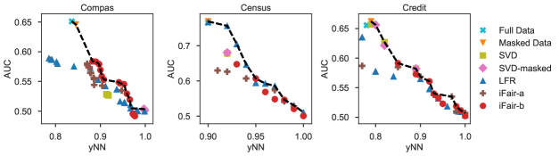
Figure 3: Plots of utility vs. individual fairness trade-off for classification task. Dashed lines represent Pareto-optimal points.

Tuning	Method	Compas					Census					Credit
		Acc	AUC	EqOpp	Parity	yNN	Acc	AUC	EqOpp	Parity	yNN	Acc	AUC	EqOpp	Parity	yNN
Baseline	Full Data	0.66	0.65	0.70	0.72	0.84	0.84	0.77	0.90	0.81	0.90	0.74	0.66	0.82	0.81	0.78
Max	LFR	0.60	0.59	0.60	0.62	0.79	0.81	0.77	0.81	0.75	0.90	0.71	0.64	0.78	0.77	0.77
Utility	iFair-a	0.60	0.58	0.91	0.91	0.87	0.78	0.63	0.96	0.91	0.91	0.69	0.61	0.84	0.86	0.74
(a)	iFair-b	0.59	0.58	0.84	0.84	0.88	0.78	0.65	0.78	0.85	0.93	0.73	0.59	0.97	0.98	0.85
Max	LFR	0.54	0.51	0.99	0.99	0.97	0.76	0.51	1.00	0.99	1.00	0.72	0.51	0.99	0.98	0.98
Fairness	iFair-a	0.56	0.53	0.97	0.99	0.95	0.76	0.51	0.95	1.00	0.99	0.73	0.53	0.99	0.98	0.97
(b)	iFair-b	0.55	0.52	0.98	1.00	0.97	0.76	0.52	0.98	0.99	0.99	0.72	0.51	0.99	1.00	0.99
	LFR	0.59	0.57	0.72	0.77	0.88	0.78	0.76	0.94	0.74	0.92	0.71	0.64	0.78	0.77	0.77
Optimal	iFair-a	0.60	0.58	0.91	0.91	0.87	0.77	0.63	0.93	0.90	0.92	0.73	0.57	0.94	0.94	0.90
(c)	iFair-b	0.59	0.58	0.83	0.84	0.89	0.78	0.65	0.78	0.85	0.93	0.73	0.59	0.97	0.98	0.85

TABLE III: Comparison of IFR vs iFair for Classification task, with hyper parameter tuning for criterion (a) max utility: best AUC (b) best Individual Fairness: best consistency, and (c) “Optimal”: best harmonic mean of AUC and consistency.

This section evaluates the effectiveness of iFair and its competitors on a classification task. We focus on the utility-(individual)fairness tradeoff that learned representations alleviate when used to train classifiers. For all methods, wherever applicable, hyper-parameters were tuned via grid search. Specifically, we chose the models that were Pareto-optimal with regard to AUC and yNN.

Results: Figure 3 shows the result for all methods and datasets, plotting utility (AUC) against individual fairness (yNN). The dotted lines show models that are Pareto-optimal with regard to AUC and yNN. We observe that there is a considerable amount of unfairness in the original dataset, which is reflected in the results of Full Data in Figure 3. Masked Data and the two SVD variants shows an improvement in fairness; however, there is still substantial unfairness hidden in the data in the form of correlated attributes. For the Compas dataset, which is the most difficult of the three datasets due to its dimensionality, SVD completely fails. The representations learned by LFR and iFair dominate all other methods in coping with the trade-off. iFair-b is the overall winner: it is consistently Pareto-optimal for all three datasets and all but the degenerate extreme points. For the extreme points in the trade-off spectrums, no method can achieve near-perfect utility without substantially losing fairness and no method can be near-perfectly fair without substantially losing utility.

Table III shows detailed results for three choices of tuning hyper-parameters (via grid search): (a) considering utility (AUC) only, (b) considering individual fairness (yNN) only, (e) using the harmonic mean of utility and individual fairness as tuning target. Here we focus on the LFR and iFair methods, as the other baselines do not have hyper-parameters to control trade-offs and are good only at extreme points of the objective space anyway. The results confirm and further illustrate the findings of Figure 3. The two iFair methods, tuned for the combination of utility and individual fairness (case (c)), achieve the best overall results: iFair-b shows an improvement of 6 percent in consistency, for a drop of 10 percent in Accuracy for Compas dataset. (+3.3% and -7% for Census, and +9% and -1.3% for Credit). Both variants of iFair outperform LFR by achieving significantly better individual fairness, with on-par or better values for utility.

V-E Evaluation on Learning-to-Rank Task

This section evaluates the effectiveness of iFair on a regression task for ranking people on Xing and Airbnb dataset. We report ranking utility in terms of Kendall’s Tau (KT), average precision (AP), individual fairness in terms of consistency (yNN) and group fairness in terms of fraction of protected candidates in top-10 ranks (statistical parity equivalent for ranking task). To evaluate models in a real world setting, for each dataset we constructed multiple queries and corresponding ground truth rankings. In case of Xing dataset we follow Zehlike et al. [27] and use the 57 job search queries. For Airbnb dataset, we generated a set of queries based on attributes values for city, neighborhood and home type. After filtering for queries which had at least 10 listings we were left with 43 queries.

As stated in Section V-A, for the Xing dataset, the deserved score is a weighted sum of the true qualifications of an individual, that is, work experience, education experience and number of profile views. To test the sensitivity of our results for different choices of weights, we varied the weights over a grid of values in $[0.0,0.25,0.5,0.75,1.0]$. We observe that the choice of weights has no significant effect on the measurs of interest. Table IV shows details. For the remainder of this section, the reported results correspond to uniform weights.

Weights			Base-rate	MAP	KT	yNN	% Protected
$\alpha_{work}$	$\alpha_{edu}$	$\alpha_{views}$	Protected				in output
0.00	0.50	1.00	33.57	0.76	0.58	1.00	31.07
0.25	0.75	0.00	33.57	0.83	0.69	0.95	35.54
0.50	1.00	0.25	32.68	0.74	0.56	1.00	31.07
0.75	0.00	0.50	32.68	0.75	0.55	1.00	31.07
0.75	0.25	0.00	31.25	0.84	0.74	0.96	33.57
1.00	0.25	0.75	32.86	0.75	0.56	1.00	31.07
1.00	1.00	1.00	32.68	0.76	0.57	1.00	31.07

TABLE IV: Experimental results on sensitivity of iFair to weights in ranking scores for Xing dataset.

Note that the baseline LFR used for the classification experiment, is not geared for regression tasks and thus omitted here. Instead, we compare iFair against the FA*IR method of Zehlike et al. [27], which is specifically designed to incorporate group fairness into rankings.

Baseline FA*IR: This ranking method takes as input a set of candidates ranked according to a precomputed score, and returns a ranked permutation which satisfies group fairness without making any changes to the scores of the candidates. Since one cannot measure consistency directly on rankings, we make a minor modification to FA*IR such that it also returns fair scores along with a fair ranking. To this end, we feed masked data to a linear regression model and compute a score for each candidate. FA*IR operates on two priority queues (sorted by previously computed scores): $P_{0}$ for non-protected candidates and $P_{1}$ for protected candidates. For each rank k, it computes the minimum number of protected candidates required to satisfy statistical parity (via significance tests) at position k. If the parity constraint is satisfied, it chooses the best candidate and its score from $P_{0}$ $\cup$ $P_{1}$. If the constraint is not satisfied, it chooses the best candidate from P1 for the next rank and leaves a placeholder for the score. Our extension linearly interpolates the scores to fill the placeholders, and thus returns a ranked list along with “fair scores”.

Results: Table V shows a comparison of experimental results for the ranking task for all methods across all datasets. We report mean values of average precision (MAP), Kendall’s Tau (KT) and consistency (yNN) over all 57 job search queries for Xing and 43 house listing queries for Airbnb. Similar to the classification task, Full Data and Masked Data have the best utility (MAP and KT), whereas iFair has the best individual fairness (yNN). iFair clearly outperforms both variants of SVD by achieving significantly better individual fairness (yNN) for comparable values of utility. As expected, FA*IR, which optimizes to satisfy statistical parity across groups, has the highest fraction of protected candidates in the top 10 ranks, but does not achieve any gains on individual fairness. This is not surprising, though, given its design goals. It also underlines our strategic point that individual fairness needs to be explicitly taken care of as a first-order objective. Between FA*IR and iFair, there is no clear winner, given their different objectives. We note, though, that the good utility that FA*IR achieves in some configurations critically hinges on the choice of the value for its parameter $p$.

Dataset	Method	MAP	KT	yNN	% Protected
		(AP@10)	(mean)	(mean)	in top $10$
	Full Data	1.00	1.00	0.93	32.50
	Masked Data	1.00	1.00	0.93	32.68
	SVD	0.74	0.59	0.81	31.79
Xing	SVD-masked	0.67	0.50	0.78	32.86
(57 queries)	FA*IR (p = 0.5)	0.93	0.94	0.92	38.21
	FA*IR (p = 0.9)	0.78	0.78	0.85	48.57
	iFair-b	0.76	0.57	1.00	31.07
	Full Data	0.68	0.53	0.72	47.44
	Masked Data	0.67	0.53	0.72	47.44
	SVD	0.66	0.49	0.73	48.37
Airbnb	SVD-masked	0.66	0.49	0.73	48.37
(43 queries)	FA*IR (p = 0.5)	0.67	0.52	0.72	48.60
	FA*IR (p = 0.6)	0.65	0.51	0.73	51.16
	iFair-b	0.60	0.45	0.80	49.07

TABLE V: Experimental results for ranking task. Reported values are means over multiple query rankings for the criterion “Optimal”: best harmonic mean of MAP and yNN.

V-F Information Obfuscation & Relation to Group Fairness

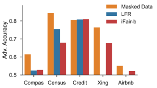
Figure 4: Adversarial accuracy of predicting protected group membership. The lower the better.

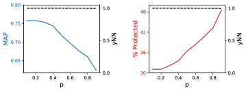
(a) Xing

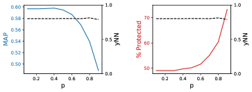
(b) Airbnb

Figure 5: Applying FA*IR algorithm to iFair representations.

We also investigate the ability of our model to obfuscate information about protected attributes. A reasonable proxy to measure the extent to which protected information is still retained in the iFair representations is to predict the value of the protected attribute from the learned representations. We trained a logistic-regression classifier to predict the protected group membership from: (i) Masked Data (ii) learned representations via LFR, and (iii) learned representations via iFair-b.

Results: Figure 4 shows the adversarial accuracy of predicting the protected group membership for all 5 datasets (with LFR not applicable to Xing and Airbnb). For all datasets, iFair manages to substantially reduce the adversarial accuracy. This signifies that its learned representations contain little information on protected attributes, despite the presence of correlated attributes. In contrast, Masked Data still reveals enough implicit information on protected groups and cannot prevent the adversarial classifier from achieving fairly good accuracy.

Relation to Group Fairness: Consider the notions of group fairness defined in Section V-C. Statistical parity requires the probability of predicting positive outcome to be independent of the protected attribute: $P(\hat{Y}=1|S=1)=P(\hat{Y}=1|S=0)$. Equality of opportunity requires this probability to be independent of the protected attribute conditioned on the true outcome $Y$: $P(\hat{Y}=1|S=1,Y=1)=P(\hat{Y}=1|S=0,Y=1)$. Thus, forgetting information about the protected attribute indirectly helps improving group fairness; as algorithms trained on the individually fair representations carry largely reduced information on protected attributes. This argument is supported by our empirical results on group fairness for all datasets. In Table III, although group fairness is not an explicit goal, we observe substantial improvements by more than 10 percentage points; the performance for other datasets is similar.

However, the extent to which iFair also benefits group fairness criteria depends on the base rates $P(Y=1|S=1)$ and $P(Y=1|S=0)$ of the underlying data. Therefore, in applications where statistical parity is a legal requirement, additional steps are needed, as discussed next.

Enforcing parity: By its application-agnostic design, it is fairly straightforward to enhance iFair by post-processing steps to enforce statistical parity, if needed. Obviously, this requires access to the values of protected attributes, but this is the case for all group fairness methods.

We demonstrate the extensibility of our framework by applying the FA*IR [27] technique as a post-processing step to the iFair representations of the Xing and Airbnb data. For each dataset, we generate top-k rankings by varying the target minimum fraction of protected candidates (parameter $p$ of the FA*IR algorithm). Figure 5 reports ranking utility (MAP), percentage of protected candidates in top 10 positions, and individual fairness (yNN) for increasing values of the FA*IR parameter $p$. The key observation is that the combined model iFair + FA*IR can indeed achieve whatever the required share of protected group members is, in addition to the individual fairness property of the learned representation.

VI Conclusions

We propose iFair, a generic and versatile, unsupervised framework to perform a probabilistic transformation of data into individually fair representations. Our approach accomodates two important criteria. First, we view fairness from an application-agnostic view, which allows us to incorporate it in a wide variety of tasks, including general classifiers and regression for learning-to-rank. Second, we treat individual fairness as a property of the dataset (in some sense, like privacy), which can be achieved by pre-processing the data into a transformed representation. This stage does not need access to protected attributes. If desired, we can also post-process the learned representations and enforce group fairness criteria such as statistical parity.

We applied our model to five real-world datasets, empirically demonstrating that utility and individual fairness can be reconciled to a large degree. Applying classifiers and regression models to iFair representations leads to algorithmic decisions that are substantially more consistent than the decisions made on the original data. Our approach is the first method to compute individually fair results in learning-to-rank tasks. For classification tasks, it outperforms the state-of-the-art prior work.

VII Acknowledgment

This research was supported by the ERC Synergy Grant “imPACT” (No. 610150) and ERC Advanced Grant “Foundations for Fair Social Computing” (No. 789373).

References

- Angwin et al. [2016] J. Angwin, J. Larson, S. Mattu, and L. Kirchner, “Machine bias: There’s software used across the country to predict future criminals and it’s biased against blacks,” ProPublica, vol. 23, 2016.
- [2] A. J. Biega, K. P. Gummadi, and G. Weikum, “Equity of attention: Amortizing individual fairness in rankings,” in The 41st International ACM SIGIR Conference on Research & Development in Information Retrieval, SIGIR 2018, Ann Arbor, MI, USA, July 08-12, 2018.
- [3] T. Calders, F. Kamiran, and M. Pechenizkiy, “Building classifiers with independency constraints,” in ICDM Workshops 2009, IEEE International Conference on Data Mining Workshops, Miami, Florida, USA, 6 December 2009.
- Chouldechova [2017] A. Chouldechova, “Fair prediction with disparate impact: A study of bias in recidivism prediction instruments,” Big data, vol. 5, no. 2, 2017.
- [5] S. Corbett-Davies, E. Pierson, A. Feller, S. Goel, and A. Huq, “Algorithmic decision making and the cost of fairness,” in Proceedings of the 23rd ACM SIGKDD International Conference on Knowledge Discovery and Data Mining, Halifax, NS, Canada, August 13 - 17, 2017.
- Crawford and Calo [2016] K. Crawford and R. Calo, “There is a blind spot in AI research,” Nature, vol. 538, 2016.
- Dheeru and Karra Taniskidou [2017] D. Dheeru and E. Karra Taniskidou, “UCI machine learning repository,” 2017. [Online]. Available: http://archive.ics.uci.edu/ml
- [8] C. Dwork, M. Hardt, T. Pitassi, O. Reingold, and R. S. Zemel, “Fairness through awareness,” in Innovations in Theoretical Computer Science 2012, Cambridge, MA, USA, January 8-10, 2012.
- Edwards and Storkey [2015] H. Edwards and A. J. Storkey, “Censoring representations with an adversary,” CoRR, vol. abs/1511.05897, 2015.
- [10] M. Feldman, S. A. Friedler, J. Moeller, C. Scheidegger, and S. Venkatasubramanian, “Certifying and removing disparate impact,” in Proceedings of the 21th ACM SIGKDD International Conference on Knowledge Discovery and Data Mining, Sydney, NSW, Australia, August 10-13, 2015.
- [11] B. Fish, J. Kun, and Á. D. Lelkes, “A confidence-based approach for balancing fairness and accuracy,” in Proceedings of the 2016 SIAM International Conference on Data Mining, Miami, Florida, USA, May 5-7, 2016.
- Flores et al. [2016] A. W. Flores, K. Bechtel, and C. T. Lowenkamp, “False positives, false negatives, and false analyses: A rejoinder to machine bias: There’s software used across the country to predict future criminals. and it’s biased against blacks,” Fed. Probation, vol. 80, 2016.
- Friedler et al. [2016] S. A. Friedler, C. Scheidegger, and S. Venkatasubramanian, “On the (im)possibility of fairness,” CoRR, vol. abs/1609.07236, 2016.
- Halko et al. [2011] N. Halko, P. Martinsson, and J. A. Tropp, “Finding structure with randomness: Probabilistic algorithms for constructing approximate matrix decompositions,” SIAM Review, vol. 53, no. 2, 2011.
- [15] M. Hardt, E. Price, and N. Srebro, “Equality of opportunity in supervised learning,” in Advances in Neural Information Processing Systems 29: Annual Conference on Neural Information Processing Systems 2016, Barcelona, Spain, December 5-10, 2016.
- Joachims and Radlinski [2007] T. Joachims and F. Radlinski, “Search engines that learn from implicit feedback,” IEEE Computer, vol. 40, no. 8, 2007.
- [17] F. Kamiran, T. Calders, and M. Pechenizkiy, “Discrimination aware decision tree learning,” in ICDM 2010, The 10th IEEE International Conference on Data Mining, Sydney, Australia, 14-17 December, 2010.
- [18] T. Kamishima, S. Akaho, H. Asoh, and J. Sakuma, “Considerations on fairness-aware data mining,” in 12th IEEE International Conference on Data Mining Workshops, ICDM Workshops, Brussels, Belgium, December 10, 2012.
- [19] J. M. Kleinberg, S. Mullainathan, and M. Raghavan, “Inherent trade-offs in the fair determination of risk scores,” in 8th Innovations in Theoretical Computer Science Conference, ITCS 2017,Berkeley, CA, USA, January 9-11, 2017.
- [20] M. J. Kusner, J. R. Loftus, C. Russell, and R. Silva, “Counterfactual fairness,” in Advances in Neural Information Processing Systems 30: Annual Conference on Neural Information Processing Systems 2017,, Long Beach, CA, USA, 4-9 December, 2017.
- Liu and Nocedal [1989] D. C. Liu and J. Nocedal, “On the limited memory BFGS method for large scale optimization,” Math. Program., vol. 45, no. 1-3, 1989.
- Louizos et al. [2015] C. Louizos, K. Swersky, Y. Li, M. Welling, and R. S. Zemel, “The variational fair autoencoder,” CoRR, vol. abs/1511.00830, 2015.
- [23] D. Pedreschi, S. Ruggieri, and F. Turini, “Discrimination-aware data mining,” in Proceedings of the 14th ACM SIGKDD International Conference on Knowledge Discovery and Data Mining, Las Vegas, Nevada, USA, August 24-27, 2008.
- Singh and Joachims [2018] A. Singh and T. Joachims, “Fairness of exposure in rankings,” CoRR, vol. abs/1802.07281, 2018.
- [25] K. Yang and J. Stoyanovich, “Measuring fairness in ranked outputs,” in Proceedings of the 29th International Conference on Scientific and Statistical Database Management, Chicago, IL, USA, June 27-29, 2017.
- [26] M. B. Zafar, I. Valera, M. Gomez-Rodriguez, and K. P. Gummadi, “Fairness beyond disparate treatment & disparate impact: Learning classification without disparate mistreatment,” in Proceedings of the 26th International Conference on World Wide Web, WWW 2017, Perth, Australia, April 3-7, 2017.
- [27] M. Zehlike, F. Bonchi, C. Castillo, S. Hajian, M. Megahed, and R. A. Baeza-Yates, “Fa*ir: A fair top-k ranking algorithm,” in Proceedings of the 2017 ACM on Conference on Information and Knowledge Management, CIKM 2017, Singapore, November 06 - 10, 2017.
- [28] R. S. Zemel, Y. Wu, K. Swersky, T. Pitassi, and C. Dwork, “Learning fair representations,” in Proceedings of the 30th International Conference on Machine Learning, ICML 2013, Atlanta, GA, USA, 16-21 June, 2013.
- Zhang and Neill [2016] Z. Zhang and D. B. Neill, “Identifying significant predictive bias in classifiers,” CoRR, vol. abs/1611.08292, 2016.