Impact of vector leptoquark on $\bar{B}\to\bar{K}^{*}l^{+}l^{-}$ anomalies

Abstract

Motivated by the recent measurement of the lepton flavour nonuniversality ratio $R_{K^{*}}$ by the LHCb Collaboration, we study the implications of vector leptoquarks on the observed anomalies associated with the $\bar{B}\to\bar{K}^{*}l^{+}l^{-}$ decay processes. The leptoquark couplings are constrained from the measured branching ratios of $B_{s}\to l^{+}l^{-}$, $K_{L}\to l^{+}l^{-}$ and $B_{s}\to\mu^{\mp}e^{\pm}$ processes. Using these constrained couplings, we estimate the branching ratios, forward-backward and lepton polarization asymmetries and also the form factor independent optimized observables ($P_{i}^{(\prime)}$) for $\bar{B}\to\bar{K}^{*}l^{+}l^{-}$ modes in the high recoil limit. We also study the other lepton flavour universality violating observables, such as $Q_{F_{L,T}}$, $Q_{i}$ and $B_{5,6s}$, where $i=1,2,\cdots 6,8$. Furthermore, we investigate the lepton flavour violating $K_{L}\to\mu^{\mp}e^{\pm}$ decay process in this model.

I Introduction

In recent times $B$ physics is going through a challenging phase, several anomalies at the level of $(3-4)\sigma$ RK-exp ; RDstar-LHCb ; RKstar-exp ; phi-decayrate ; Kstar-decayrate ; P5p ; isospin-kstar have been observed by the LHCb Collaboration in the rare flavour changing neutral current (FCNC) processes involving the quark level transition $b\to sl^{+}l^{-}$. As these processes are one-loop suppressed in the standard model (SM), they may play a vital role to decipher the signature of new physics (NP) beyond it. To supplement these observations, recently LHCb has reported $2.2\sigma$ and $2.4\sigma$ discrepancies in the measurement of $R_{K^{*}}$ observable in the dilepton invariant mass squared bins $q^{2}\in[0.045,1.1]~{}{\rm GeV}^{2}$ and $q^{2}\in[1.1,6.0]~{}{\rm GeV}^{2}$ RKstar-exp , which are in the same line as the previous result on the violation of lepton universality parameter $R_{K}$ RK-exp . Also the lepton nonuniversality (LNU) parameters in the $B\to D^{(*)}$ processes ($R_{D^{(*)}}$) have been measured by Belle, BaBar and LHCb collaborations, which have respectively $1.9\sigma$ RD-BaBar ; RD-exp and $3.3\sigma$ RDstar-LHCb ; RD-exp deviations from their corresponding SM predictions. In Table I, we present the observed LNU ratios, associated with the $b\to sl^{+}l^{-}$ and $b\to cl\nu_{l}$ processes at LHCb and $B$ factories. Furthermore, the decay rate of $B_{s}\to\phi\mu^{+}\mu^{-}$ process phi-decayrate also has discrepancy of around $3\sigma$ in the low $q^{2}$ region.

Table 1: The LNU parameters observed by the LHCb collaboration and the $B$ factories.

LNU parameters	SM predictions	Expt. result	Deviation
$R_{K}|_{q^{2}\in[1.0,6.0]}$	$1.0003\pm 0.0001$ RK-SM	$0.745^{+0.090}_{-0.074}\pm 0.036$ RK-exp	$2.6\sigma$
$R_{K^{*}}|_{q^{2}\in[0.045,1.1]}$	$0.92\pm 0.02$  RKstar-SM	$0.66^{+0.11}_{-0.07}\pm 0.03$ RKstar-exp	$2.2\sigma$
$R_{K^{*}}|_{q^{2}\in[1.1,6.0]}$	$1.00\pm 0.01$ RKstar-SM	$0.69^{+0.11}_{-0.07}\pm 0.05$  RKstar-exp	$2.4\sigma$
$R_{D}$	$0.300\pm 0.008$ RD-SM	$0.397\pm 0.040\pm 0.028$  RD-exp	$1.9\sigma$
$R_{D^{*}}$	$0.252\pm 0.003$  RDstar-SM	$0.316\pm 0.016\pm 0.010$ RD-exp	$3.3\sigma$

In this context, we would like to investigate whether the observed anomalies in the rare $\bar{B}\to\bar{K}^{*}l^{+}l^{-}$ decay processes, mediated through $b\to sl^{+}l^{-}$ transitions, can be explained in the vector leptoquark model. In the last few years, these processes have provided several surprising results and played a very crucial role to look for NP signals, as the measurement of four-body angular distribution provides a large number of observables which can be used to probe NP signature. In the low $q^{2}\in[1,6]~{}{\rm GeV}^{2}$ region (where $q^{2}$ denotes the dilepton invariant mass square), the theoretical predictions for such observables are very precise and generally free from the hadronic uncertainties. However, the observed forward-backward asymmetry is systematically below the corresponding SM prediction, though the zero crossing point is consistent with it. Moreover, the LHCb Collaboration has reported many other deviations from the SM expectations in the angular observables. The largest discrepancy of $\sim 3\sigma$ in the famous $P_{5}^{\prime}$ optimized observable P5p and the decay rate Kstar-decayrate of these processes provide a sensitive probe to explore NP effects in $b\to s\gamma$, $b\to sll$ transitions. In addition, the isospin asymmetry isospin-kstar is also measured by the LHCb experiment in the full $q^{2}$ region, which can be used to probe the NP signal. For the first time, recently Belle has measured two new lepton flavour universality violating (LFUV) observables $Q_{4,5}=P_{4,5}^{\mu^{\prime}}-P_{4,5}^{e^{\prime}}$ Q4-Belle . In order to scrutinize the above results, these processes have already been investigated in the context of various new physics models and also in model-independent ways. The recent measurement on the $R_{K^{*}}$ parameter at LHCb experiment has drawn much attention to restudy these processes in the low $q^{2}$ region. In the light of recent $R_{K^{*}}$ data, several works recent-arXiv , have been reported in the literature recently.

To understand the origin of the current issues observed at LHCb experiment in a particular theoretical framework, here we extend the SM by adding a single vector leptoquark (LQ) and reinvestigate the rare semileptonic $\bar{B}\to\bar{K}^{*}l^{+}l^{-}$ decay processes. Though there are a few recent studies in the literature recent-arXiv , which have investigated $R_{K^{*}}$ anomalies but no analysis of $R_{K^{*}}$ has been done with vector LQ, which can induce the process at tree level. In our previous work mohanta0 , we have made a comparative study of the rare semileptonic $\bar{B}\to\bar{K}^{*}l^{+}l^{-}$ decay modes in both the $(3,2,7/6)$ and $(3,2,1/6)$ scalar LQ models. However, we have not investigated the new $R_{K^{*}}$, $Q_{4,5}$ and $Q_{F_{L,T}}$ observables. The model-independent analysis of these new set of observables can be found in Ref. kstar-Q4 . The motivation of this work is to check how the angular analysis of $\bar{B}\to\bar{K}^{*}l^{+}l^{-}$ processes in the context of vector LQ could help establishing the possible existence of NP from the above discussed anomalies. LQs are hypothetical color triplet bosonic particles, which arise naturally from the unification of quarks and leptons, and carry both the lepton and baryon numbers. They can be either scalar (spin 0) or vector (spin 1) in nature. The presence of vector LQs at the TeV scale can be found in many extended SM theories such as grand unified theories based on $SU(5)$, $SO(10)$, etc. GUT ; Pati , Pati-Salam model Pati ; Pati-salam , composite model Composite and the technicolor model Technicolor . The baryon number conserving LQs avoid proton decay and could be light enough to be seen in the current experiments. Thus, in this work, we consider the singlet $(3,1,2/3)$ vector LQ, which is invariant under the SM $SU(3)_{C}\times SU(2)_{L}\times U(1)_{Y}$ gauge group and conserves both the baryon and lepton numbers. In addition to the (axial)vector operators, this LQ also provides additional (pseudo)scalar operators to the SM. We compute the branching ratios, forward-backward asymmetries, polarization asymmetries and the form factor independent (FFI) observables $(P_{i}^{(\prime)})$ of the $\bar{B}\to\bar{K}^{*}l^{+}l^{-}$ processes in this model. In this paper, we mainly focus on the $R_{K^{*}}$ anomaly and the additional observables related to the lepton flavour violation in order to confirm or rule out the presence of lepton nonuniversality in the rare $B$ meson decays. We also investigate the $Q_{i}$, $Q_{F_{L,T}}$ and $B_{i}$ observables in the context of vector LQ, so as to reveal the possible interplay of NP. In the literature, the observed anomalies at LHCb experiment in various rare decays of $B$ mesons have been studied in the LQ model mohanta0 ; mohanta1 ; mohanta2 ; mohanta3 ; davidson ; kosnik-LQ ; KL-LQ .

The paper is organized as follows. In section II, we discuss the effective Hamiltonian responsible for the $b\to sl^{+}l^{-}$ processes and the new physics contributions arising due to the exchange of vector LQ. In section III, we show the constraints on LQ couplings from the branching ratios of rare $B_{s}\to l^{+}l^{-}$, $K_{L}\to l^{+}l^{-}$ and $B_{s}\to\mu^{\mp}e^{\pm}$ processes. The branching ratios, forward-backward asymmetries, lepton polarizations and the CP violating parameters in the $\bar{B}\to\bar{K}^{*}l^{+}l^{-}$ processes are calculated in section IV. Section V deals with the lepton flavour violating decay $K_{L}\to\mu^{\mp}e^{\pm}$ and section VI contains the summary.

II Generalized effective Hamiltonian

In the SM, the most general effective Hamiltonian responsible for the quark level transitions $b\to sl^{+}l^{-}$ is given by b-s-Hamiltonian

$${\cal H}_{\rm eff} = -\frac{4G_{F}}{\sqrt{2}}V_{tb}V_{ts}^{*}\Bigg{[}\sum_{i=1}^{6}C_{i}(\mu)\mathcal{O}_{i}+C_{7}\frac{e}{16\pi^{2}}\Big{(}\bar{s}\sigma_{\mu\nu}(m_{s}P_{L}+m_{b}P_{R})b\Big{)}F^{\mu\nu}$$ (1)

$$+\frac{\alpha}{4\pi}\left(C_{9}^{\rm eff}(\bar{s}\gamma^{\mu}P_{L}b)(\bar{l}\gamma_{\mu}l)+C_{10}(\bar{s}\gamma^{\mu}P_{L}b)(\bar{l}\gamma_{\mu}\gamma_{5}l)\right)\Bigg{]}\;,$$

where $G_{F}$ is the Fermi constant, $V_{qq^{\prime}}$ are the Cabibbo-Kobayashi-Maskawa (CKM) matrix elements, $\alpha$ is the fine structure constant and $P_{L,R}=(1\mp\gamma_{5})/2$ are the chiral projection operators. Here $\mathcal{O}_{i}$’s are the six dimensional operators and $C_{i}$’s are the corresponding Wilson coefficients, evaluated at the renormalization scale $\mu=m_{b}$ b-s-Wilson .

II.1 Contributions from vector leptoquark

The SM effective Hamiltonian (1) can be modified by adding a single vector LQ and will give measurable deviations from the corresponding SM predictions in the $B$ sector. Here we consider $V^{1}(3,1,2/3)$ singlet vector LQ which is invariant under the SM gauge group $SU(3)_{C}\times SU(2)_{L}\times U(1)_{Y}$. In order to avoid rapid proton decay, we assume that the LQ conserves both baryon and lepton numbers. The baryon number conserving vector LQs can have sizeable Yukawa couplings and could be light enough to be accessible in a current collider. The $V^{1}(3,1,2/3)$ LQ could potentially contribute to the $b\to sl^{+}l^{-}$ processes and one can constrain the corresponding LQ couplings from the experimental data on $B_{s}\to l^{+}l^{-}$ processes.

The interaction Lagrangian for $V^{1}(3,1,2/3)$ leptoquark is given by kosnik-LQ ; mohanta3

$$\mathcal{L}^{(1)}=\left(g_{L}\,\overline{Q}_{L}\gamma^{\mu}L_{L}+g_{R}\,\overline{d_{R}}\gamma^{\mu}l_{R}\right)\,V^{1}_{\mu}+{\rm h.c.},$$ (2)

where $Q_{L}~{}(L_{L})$ is the left-handed quark (lepton) doublets and $d_{R}~{}(l_{R})$ is the right-handed down-type quark (charged-lepton) singlets. Here $g_{L}$ is the coupling of vector LQ with the quark and lepton doublets and $g_{R}$ is the LQ coupling with down-type quarks and the right-handed leptons. To keep the notations clean, the leptoquark couplings $g_{L}$ and $g_{R}$ are considered in the mass basis of down-type quarks, i.e., the couplings $g_{L}$ and $g_{R}$ are rotated and expressed in the quark mass basis by the redefinition $U_{L}^{\dagger}g_{L}\rightarrow g_{L}$ and $U_{R}^{\dagger}g_{R}\rightarrow g_{R}$, where $U_{L,R}$ connect the mass and gauge bases, i.e., $d_{L,R}^{\rm gauge}=U_{L,R}d_{L,R}^{\rm mass}$. The interaction Lagrangian (2) provides in addition to the vector ($C_{9}^{(\prime)\rm LQ}$) and axial-vector ($C_{10}^{(\prime)\rm LQ}$) new Wilson coefficients, new scalar $C_{S}^{(\prime)\rm LQ}$ and pseudoscalar $C_{P}^{(\prime)\rm LQ}$ coefficients, and is thus non-chiral in nature. The new Wilson coefficients are related to the LQ couplings through the following relations kosnik-LQ ; mohanta3

$$C_{9}^{\rm LQ}=-C_{10}^{\rm LQ}=\frac{\pi}{\sqrt{2}G_{F}V_{tb}V_{ts}^{*}\alpha}\frac{(g_{L})_{sl}(g_{L})^{*}_{bl}}{M_{\rm LQ}^{2}}\,,$$ (3a)

$$C_{9}^{\prime\rm LQ}=C_{10}^{\prime\rm LQ}=\frac{\pi}{\sqrt{2}G_{F}V_{tb}V_{ts}^{*}\alpha}\frac{(g_{R})_{sl}(g_{R})^{*}_{bl}}{M_{\rm LQ}^{2}}\,,$$ (3b)

$$-C_{P}^{\rm LQ}=C_{S}^{\rm LQ}=\frac{\sqrt{2}\pi}{G_{F}V_{tb}V_{ts}^{*}\alpha}\frac{(g_{L})_{sl}(g_{R})^{*}_{bl}}{M_{\rm LQ}^{2}}\,,$$ (3c)

$$C_{P}^{\prime\rm LQ}=C_{S}^{\prime\rm LQ}=\frac{\sqrt{2}\pi}{G_{F}V_{tb}V_{ts}^{*}\alpha}\frac{(g_{R})_{sl}(g_{L})^{*}_{bl}}{M_{\rm LQ}^{2}}\,.$$ (3d)

III Constraint on the vector leptoquark couplings

After knowing about the interplay of possible new Wilson coefficients, we now proceed to constrain the new physics parameters by comparing the theoretical and experimental results on various rare $B(K)$ meson decays.

III.1 $B_{s}\to l^{+}l^{-}$ processes

In this subsection, we show the constraints on the new LQ couplings from the $B_{s}\to l^{+}l^{-}$ processes, as these new coefficients also contribute to the $B_{s}\to l^{+}l^{-}$ processes. These decay processes are very rare in the SM as they occur at loop level and further suffer from helicity suppression. The only non-perturbative quantity involved is the decay constant of $B$ mesons, which can be reliably calculated by using the non-perturbative methods, thus, these processes are theoretically very clean. In the SM, only the $C_{10}^{\rm SM}$ Wilson coefficient contributes to the branching ratio.

The branching ratios of $B_{s}\to l^{+}l^{-}$ processes in the vector LQ model are given by Buras

$${\rm BR}(B_{s}\to l^{+}l^{-})=\frac{G_{F}^{2}}{16\pi^{3}}\tau_{B_{s}}\alpha^{2}f_{B_{s}}^{2}M_{B_{s}}m_{l}^{2}|V_{tb}V_{ts}^{*}|^{2}\left|C_{10}^{\rm SM}\right|^{2}\sqrt{1-\frac{4m_{l}^{2}}{M_{B_{s}}^{2}}}\times\left(|P|^{2}+|S|^{2}\right),$$ (4)

where $P$ and $S$ parameters are defined as

$$P\equiv\frac{C_{10}^{\rm SM}+C_{10}^{\rm LQ}-C_{10}^{\prime\rm LQ}}{C_{10}^{\rm SM}}+\frac{M_{B_{s}}^{2}}{2m_{l}}\Big{(}\frac{m_{b}}{m_{b}+m_{s}}\Big{)}\Big{(}\frac{C_{P}^{\rm LQ}-C_{P}^{\prime\rm LQ}}{C_{10}^{\rm SM}}\Big{)},$$

$$S\equiv\sqrt{1-\frac{4m_{l}^{2}}{M_{B_{s}}^{2}}}\frac{M_{B_{s}}^{2}}{2m_{l}}\Big{(}\frac{m_{b}}{m_{b}+m_{s}}\Big{)}\Big{(}\frac{C_{S}^{\rm LQ}-C_{S}^{\prime\rm LQ}}{C_{10}^{\rm SM}}\Big{)}.$$ (5)

Now to compare the theoretical branching ratios with the experimental results, one can define the parameter $R_{q}$, which is the ratio of branching fraction to its SM value as

$$R_{q}=\frac{{\rm BR}(B_{s}\to l^{+}l^{-})}{{\rm BR}^{\rm SM}(B_{s}\to l^{+}l^{-})}=|P|^{2}+|S|^{2}.$$ (6)

Using Eqn. (6), we constrain the new couplings by comparing the SM predicted branching ratios Bobeth of $B_{s}\to l^{+}l^{-}$ processes with their corresponding experimental results e-br ; mu-br ; tau-br . The constraint on vector LQ couplings from $B_{s}\to l^{+}l^{-}$ processes has already been extracted in mohanta1 ; mohanta3 , therefore, here we will simply quote the results. In Table II, we have presented the obtained bound on the $(g_{L})_{sl}(g_{L})^{*}_{bl}$ leptoquark couplings. The constraints on the combination of $C_{S}^{(\prime)\rm LQ}$ Wilson coefficients i.e., $C_{S}^{\rm LQ}\pm C_{S}^{\prime\rm LQ}$ are presented in Table III, from which one can obtain the bound on individual $C_{S}^{(\prime)\rm LQ}$ Wilson coefficients.

III.2 $K_{L}\to l^{+}l^{-}$ processes

The effective Hamiltonian responsible for the $s\to dl^{+}l^{-}$ quark level transitions in the SM is given by KL-2

$$\mathcal{H}_{\rm eff} = \frac{G_{F}}{\sqrt{2}}\frac{\alpha}{2\pi\sin^{2}\theta_{W}}\left(\lambda_{c}Y_{NL}+\lambda_{t}Y(x_{t})\right)\left(\bar{s}\gamma^{\mu}(1-\gamma_{5})d\right)\left(\bar{l}\gamma_{\mu}(1-\gamma_{5})l\right)$$ (7)

$$= \frac{G_{F}}{\sqrt{2}}\frac{\alpha}{2\pi}\lambda_{u}C^{\rm SM}_{K}\left(\bar{s}\gamma^{\mu}(1-\gamma_{5})d\right)\left(\bar{l}\gamma_{\mu}(1-\gamma_{5})l\right),$$ (8)

where $\lambda_{i}=V_{id}V_{is}^{*}$, $x_{t}=m_{t}^{2}/M_{W}^{2}$, $\sin^{2}\theta_{W}=0.23$ and $C^{\rm SM}_{K}$ is the SM Wilson coefficient given as

$$C^{\rm SM}_{K}=\frac{\left(\lambda_{c}Y_{NL}+\lambda_{t}Y(x_{t})\right)}{\sin^{2}\theta_{W}\lambda_{u}}\;.$$ (9)

Here the functions $Y_{NL}$ and $Y(x_{t})$ KL-3 are the contributions from the charm and top quark respectively. The estimated branching ratio of the short distance (SD) part of the $K_{L}\to\mu^{+}\mu^{-}$ process is ${\rm BR}(K_{L}\to\mu^{+}\mu^{-})|_{\rm SD}<2.5\times 10^{-9}$ KL-1 .

Including the $(3,1,2/3)$ vector LQ contributions, the total branching ratios of $K_{L}\to l^{+}l^{-}$ processes are given by mohanta3

$${\rm BR}(K_{L}\to l^{+}l^{-})=\frac{G_{F}^{2}}{8\pi^{3}}\tau_{K_{L}}\alpha^{2}f_{K}^{2}M_{K}m_{l}^{2}|\lambda_{u}|^{2}\left|C_{\rm SM}^{K}\right|^{2}\sqrt{1-\frac{4m_{l}^{2}}{M_{K}^{2}}}\times\left(|P_{K}|^{2}+|S_{K}|^{2}\right),$$ (10)

where $P_{K}$ and $S_{K}$ parameters have analogous expressions as Eqn. (5) with the replacement of $M_{B_{s}}\to M_{K}$ and the corresponding new Wilson coefficients by $C_{iK}^{\rm LQ}$, which are given as mohanta3

$$C_{10K}^{\rm LQ}=-\frac{\pi}{G_{F}\alpha\lambda_{u}}\frac{{\rm Re}[(g_{L})_{dl}(g_{L})_{sl}^{*}]}{M_{\rm LQ}^{2}}\;,$$ (11a)

$$C_{10K}^{\prime\rm LQ}=-\frac{\pi}{G_{F}\alpha\lambda_{u}}\frac{{\rm Re}[(g_{R})_{dl}(g_{R})_{sl}^{*}]}{M_{\rm LQ}^{2}}\;,$$ (11b)

$$C_{SK}^{\rm LQ}=-C_{PK}^{\rm LQ}=\frac{\pi}{2G_{F}\alpha\lambda_{u}}\frac{{\rm Re}[(g_{L})_{dl}(g_{R})_{sl}^{*}]}{M_{\rm LQ}^{2}}\;,$$ (11c)

$$C_{SK}^{\prime\rm LQ}=C_{PK}^{\prime\rm LQ}=\frac{\pi}{2G_{F}\alpha\lambda_{u}}\frac{{\rm Re}[(g_{R})_{dl}(g_{L})_{sl}^{*}]}{M_{\rm LQ}^{2}}\;.$$ (11d)

Now using the experimental upper limits pdg on the branching ratios of $K_{L}\to l^{+}l^{-}$ decay processes, the constraint on the new physics parameters are extracted in Ref. mohanta3 . In Table II, we present the constraints on $(g_{L})_{dl}(g_{L})_{sl}^{*}$ couplings, and the bound on $C_{S}^{\rm LQ}\pm C_{S}^{\prime\rm LQ}$ Wilson coefficients are given in Table III.

Table 2: Constraints on the LQ couplings obtained from various leptonic $B_{s}\to l^{+}l^{-}$ and $K_{L}\to l^{+}l^{-}$ decay processes .

Decay Process	Couplings involved	Upper bound of
		the couplings
$B_{s}\to e^{\pm}e^{\mp}$	$|(g_{L})_{se}(g_{L})^{*}_{be}|$	$<~{}11.8$
$B_{s}\to\mu^{\pm}\mu^{\mp}$	$|(g_{L})_{s\mu}(g_{L})^{*}_{b\mu}|$	$\leq 2.3\times 10^{-3}$
$K_{L}\to e^{\pm}e^{\mp}$	$|(g_{L})_{de}(g_{L})^{*}_{se}|$	$(1.3-2.35)\times 10^{-3}$
$K_{L}\to\mu^{\pm}\mu^{\mp}$	$|(g_{L})_{d\mu}(g_{L})^{*}_{s\mu}|$	$(1.4-1.5)\times 10^{-4}$

Table 3: Constraint on combinations of $C_{S(K)}^{(\prime)\rm LQ}$ Wilson coefficients from rare leptonic $B_{s}\to l^{+}l^{-}$ and $K_{L}\to l^{+}l^{-}$ decay processes.

Decay Process	Bound on $C_{S(K)}^{\rm LQ}+C_{S(K)}^{\prime\rm LQ}$	Bound on $C_{S(K)}^{\rm LQ}-C_{S(K)}^{\prime\rm LQ}$
$B_{s}\to e^{\pm}e^{\mp}$	$-1.4\to 1.4$	$-1.4\to 1.4$
$B_{s}\to\mu^{\pm}\mu^{\mp}$	$0.0\to 0.32$	$0.1\to 0.18$
$K_{L}\to e^{\pm}e^{\mp}$	$(-2.0\to 2.0)\times 10^{-4}$	$(1.25\to 2)\times 10^{-4}$
$K_{L}\to\mu^{\pm}\mu^{\mp}$	$(-6.0\to 3.0)\times 10^{-3}$	$(0.05\to 5.6)\times 10^{-3}$

III.3 $B_{s}\to\mu^{\mp}e^{\pm}$ process

The constraints on LQ couplings obtained from the branching ratio of the lepton flavor violating (LFV) $B_{s}\to\mu^{\mp}e^{\pm}$ process is discussed in this subsection. In the SM, the LFV decay modes occur at loop level with the presence of tiny neutrinos in one of the loops or proceed via box diagrams. However, these processes can occur at tree level in the vector LQ model. The present experimental upper bound on the branching ratio of $B_{s}\to\mu^{\mp}e^{\pm}$ process is pdg

$${\rm BR}(B_{s}\to\mu^{\mp}e^{\pm})<1.1\times 10^{-8}.$$ (12)

In the presence of $V^{1}(3,1,2/3)$ vector LQ, the branching ratio of $B_{s}\to\mu^{-}e^{+}$ decay mode is

$${\rm BR}(B_{s}\to\mu^{-}e^{+}) = \tau_{B_{s}}\frac{G_{F}^{2}\alpha^{2}M_{B_{s}}^{5}f_{B_{s}}^{2}|V_{tb}V_{ts}^{*}|^{2}}{64\pi^{3}}\left(1-\frac{m_{\mu}^{2}}{M_{B_{s}}^{2}}\right)^{2}\Bigg{[}\left|\frac{m_{\mu}}{M_{B_{s}}^{2}}\left(G_{9}^{\rm LQ}-G_{9}^{\prime\rm LQ}\right)+\frac{G_{S}^{\rm LQ}-G_{S}^{\prime\rm LQ}}{m_{b}}\right|^{2}$$ (13)

$$+\left|\frac{m_{\mu}}{M_{B_{s}}^{2}}\left(G_{10}^{\rm LQ}-G_{10}^{\prime\rm LQ}\right)+\frac{G_{P}^{\rm LQ}-G_{P}^{\prime\rm LQ}}{m_{b}}\right|^{2}\Bigg{]}\,,$$

and the branching ratio of $B_{s}\to\mu^{+}e^{-}$ decay process is given by

$${\rm BR}(B_{s}\to e^{-}\mu^{+}) = \tau_{B_{s}}\frac{G_{F}^{2}\alpha^{2}M_{B_{s}}^{5}f_{B_{s}}^{2}|V_{tb}V_{ts}^{*}|^{2}}{64\pi^{3}}\left(1-\frac{m_{\mu}^{2}}{M_{B_{s}}^{2}}\right)^{2}\Bigg{[}\left|-\frac{m_{\mu}}{M_{B_{s}}^{2}}\left(H_{9}^{\rm LQ}-H_{9}^{\prime\rm LQ}\right)+\frac{H_{S}^{\rm LQ}-H_{S}^{\prime\rm LQ}}{m_{b}}\right|^{2}$$ (14)

$$+\left|\frac{m_{\mu}}{M_{B_{s}}^{2}}\left(H_{10}^{\rm LQ}-H_{10}^{\prime\rm LQ}\right)+\frac{H_{P}^{\rm LQ}-H_{P}^{\prime\rm LQ}}{m_{b}}\right|^{2}\Bigg{]}\,,$$

where the mass of electron is neglected. Here the new $G(H)_{a}^{(\prime)\rm LQ}~{}(a=9,10,S,P)$ coefficients have similar expression as Eqns. (3a,3b, 3c,3d) with the replacement of LQ couplings $(g_{i})_{sl}(g_{j})_{bl}^{*}\to(g_{i})_{se}(g_{j})_{b\mu}^{*}$, where $(i,j=L,R)$ for $G_{a}^{(\prime)\rm LQ}$ and $(g_{i})_{sl}(g_{j})_{bl}^{*}\to(g_{i})_{s\mu}(g_{j})_{be}^{*}$ for $H_{a}^{(\prime)\rm LQ}$ coefficients.

The total branching ratio of $B_{s}\to\mu^{\mp}e^{\pm}$ process is

$${\rm BR}(B_{s}\to\mu^{\mp}e^{\pm})={\rm BR}(B_{s}\to\mu^{-}e^{+})+{\rm BR}(B_{s}\to\mu^{+}e^{-}).$$ (15)

For chiral LQ, only $G(H)_{9,10}^{(\prime)\rm LQ}$ coefficients will be present. Now using the experimental upper limit of the branching ratio (12), we obtain the constraint on LQ couplings as

$$|(g_{L})_{se}(g_{L})_{b\mu}^{*}|<2.83\times 10^{-2}.$$ (16)

Now neglecting the $V\pm A$ couplings, the constraint on $(G_{S}^{\rm LQ}\pm G_{S}^{\prime\rm LQ})$ coefficient is shown in Fig. 1. From the figure, we find the allowed range for the above combinations of Wilson coefficients as

$$|G_{S}^{\rm LQ}-G_{S}^{\prime\rm LQ}|\leq 0.3,~{}~{}~{}|G_{S}^{\rm LQ}+G_{S}^{\prime\rm LQ}|\leq 0.3\,.$$ (17)

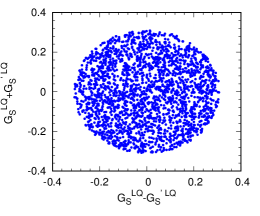
Figure 1: The constraint on $G_{S}^{\rm LQ}\pm G_{S}^{\prime\rm LQ}$ couplings obtained from the branching ratio of $B_{s}\to\mu^{-}e^{+}$ process.

IV $\bar{B}\to\bar{K}^{*}l^{+}l^{-}$ processes

In this section, we present the theoretical framework to calculate the branching ratios for the rare semileptonic $\bar{B}\to\bar{K}^{*}l^{+}l^{-}$ processes. Furthermore, the dileptons present in these processes allow one to formulate several useful observables which can be used to probe and discriminate different scenarios of NP. The full four body angular distribution of the $\bar{B}\rightarrow\bar{K}^{*0}\left(\rightarrow K^{-}\pi^{+}\right)l^{+}l^{-}$ decay processes can be described by four independent kinematic variables, $q^{2}$ and the three angles $\theta_{K^{*}},\theta_{l}$ and $\phi$. Here we assume that, $\bar{K}^{*0}\rightarrow K^{-}\pi^{+}$ is on the mass shell. The differential decay distribution of these processes with respect to the four independent variables are given as kstar-br-1 ; kstar-br-2 ; kstar-br-3

$$\frac{d^{4}\Gamma}{dq^{2}~{}d\cos\theta_{l}~{}d\cos\theta_{K^{*}}~{}d\phi}=\frac{9}{32\pi}J\left(q^{2},\theta_{l},\theta_{K^{*}},\phi\right),$$ (18)

where the lepton spins have been summed over. Here $q^{2}$ is the lepton-pair invariant mass square, $\theta_{l}$ is the angle between the negatively charged lepton and the $\bar{B}$ in the $l^{+}l^{-}$ frame, $\theta_{K^{*}}$ is defined as the angle between $K^{-}$ and $\bar{B}$ in the $K^{-}\pi^{+}$ center of mass frame and $\phi$ is the angle between the normals of the $K^{-}\pi^{+}$ and the dilepton planes. The physically allowed regions of these variables in the phase space are given by

$$4m^{2}_{l}\leqslant q^{2}\leqslant\left(m_{B}-m_{K^{*}}\right)^{2},\hskip 17.07182pt-1\leqslant\cos\theta_{l}\leqslant 1,\hskip 17.07182pt-1\leqslant\cos\theta_{K^{*}}\leqslant 1,\hskip 19.91684pt0\leqslant\phi\leqslant 2\pi,$$ (19)

where $m_{B}~{}(m_{K^{*}}$) and $m_{l}$ are respectively the masses of $B~{}(K^{*})$ meson and charged-lepton. The explicit dependence of the decay distribution on the above three angles, (i.e., the dependence $J\left(q^{2},\theta_{l},\theta_{K^{*}},\phi\right)$ function) can be written as

$$J\left(q^{2},\theta_{l},\theta_{K^{*}},\phi\right) = J^{s}_{1}\sin^{2}\theta_{K^{*}}+J^{c}_{1}\cos^{2}\theta_{K^{*}}+\left(J^{s}_{2}\sin^{2}\theta_{K^{*}}+J^{c}_{2}\cos^{2}\theta_{K^{*}}\right)\cos 2\theta_{l}$$ (20)

$$+ J_{3}\sin^{2}\theta_{K^{*}}\sin^{2}\theta_{l}\cos 2\phi+J_{4}\sin 2\theta_{K^{*}}\sin 2\theta_{l}\cos\phi+J_{5}\sin 2\theta_{K^{*}}\sin\theta_{l}\cos\phi$$

$$+ (J_{6}^{s}\sin^{2}\theta_{K^{*}}+J_{6}^{c}\cos^{2}\theta_{K^{*}})\cos\theta_{l}+J_{7}\sin 2\theta_{K^{*}}\sin\theta_{l}\sin\phi$$

$$+ J_{8}\sin 2\theta_{K^{*}}\sin 2\theta_{l}\sin\phi+J_{9}\sin^{2}\theta_{K^{*}}\sin^{2}\theta_{l}\sin 2\phi\;,$$

where the coefficients $J_{i}^{(a)}=J_{i}^{(a)}\left(q^{2}\right)$ for $i=1,....,9$ and $a=s,c$ are functions of the dilepton invariant mass. The complete expression for these coefficients in terms of the transversity amplitudes $A_{0}$, $A_{\parallel}$, $A_{\perp}$, and $A_{t}$ can be found in the Ref. kstar-br-1 ; kstar-br-2 ; kstar-fl-2 .

After performing the integration over all the angles, the decay rate of $\bar{B}\rightarrow\bar{K}^{*}l^{+}l^{-}$ processes with respect to $q^{2}$ is given by kstar-br-1

$$\frac{d\Gamma}{dq^{2}}=\frac{3}{4}\left(J_{1}-\frac{J_{2}}{3}\right),$$ (21)

where $J_{i}=2J_{i}^{s}+J_{i}^{c}$.

Previously LHCb had measured the LNU parameter in the low $q^{2}$, i.e., $(1\leq q^{2}\leq 6)~{}{\rm GeV}^{2}$ region of $B\to Kl^{+}l^{-}$ process as RK-exp

$$R_{K}^{\rm LHCb}=\frac{{\rm BR}(B^{+}\to K^{+}\mu^{+}\mu^{-})}{{\rm BR}(B^{+}\to K^{+}e^{+}e^{-})}=0.745^{+0.090}_{-0.074}\pm 0.036$$ (22)

which has $2.6\sigma$ deviation from the corresponding SM result $R_{K}^{\rm SM}=1.0003\pm 0.0001$ RK-SM . Recently, LHCb collaboration has measured analogous lepton flavour universality violating parameter, $R_{K^{*}}$, in the $\bar{B}\to\bar{K}^{*}l^{+}l^{-}$ processes in two different bins, which also have around $2\sigma$ deviations from the corresponding SM values as presented in Table-I. Besides the branching ratios and the $R_{K^{*}}$ parameter, there are many observables associated with $\bar{B}\to\bar{K}^{*}l^{+}l^{-}$ processes which could be sensitive to new physics. The interesting observables are

1. The zero crossing of the forward-backward asymmetry, which is defined as kstar-br-1

   $$A_{FB}\left(q^{2}\right) = \left[\int_{-1}^{0}d\cos\theta_{l}\frac{d^{2}\Gamma}{dq^{2}d\cos\theta_{l}}-\int_{0}^{1}d\cos\theta_{l}\frac{d^{2}\Gamma}{dq^{2}d\cos\theta_{l}}\right]\Big{/}\frac{d\Gamma}{dq^{2}}$$ (23)

   $$= -\frac{3}{8}\frac{J_{6}}{d\Gamma/dq^{2}}\;.$$

2. The longitudinal and transverse polarization fractions of the $K^{*}$ meson, in terms of the angular coefficients $(J_{i})$ can be written as kstar-fl-1 ; kstar-fl-2

   $$F_{L}\left(q^{2}\right)=\frac{3J_{1}^{c}-J_{2}^{c}}{4d\Gamma/dq^{2}}\;,\hskip 42.67912ptF_{T}\left(q^{2}\right)=1-F_{L}(q^{2})\,.$$ (24)

3. The form factor independent (FFI) optimized observables $P_{i}$’s, where $i=1,..,6,8$ are given as kstar-p1

   $$P_{1}\left(q^{2}\right) = \frac{J_{3}}{2J_{2}^{s}}\;,\hskip 42.67912ptP_{2}\left(q^{2}\right)=\beta_{l}\frac{J^{s}_{6}}{8J_{2}^{s}}\;,\hskip 42.67912ptP_{3}\left(q^{2}\right)=-\frac{J_{9}}{4J_{2}^{s}}\;,$$

   $$P_{4}\left(q^{2}\right) = \frac{\sqrt{2}J_{4}}{\sqrt{-J_{2}^{c}\left(2J_{2}^{s}-J_{3}\right)}}\;,\hskip 34.14322ptP_{5}\left(q^{2}\right)=\frac{\beta_{l}J_{5}}{\sqrt{-2J_{2}^{c}\left(2J_{2}^{s}+J_{3}\right)}}\;,$$

   $$P_{6}\left(q^{2}\right) = -\frac{\beta_{l}J_{7}}{\sqrt{-2J_{2}^{c}\left(2J_{2}^{s}-J_{3}\right)}}\;,\hskip 28.45274ptP_{8}\left(q^{2}\right)=-\frac{\beta_{l}J_{8}}{\sqrt{-2J_{2}^{c}\left(2J_{2}^{s}-J_{3}\right)}}\;.$$ (25)

4. In order to interpret the LHCb measurements more precisely, a slightly modified set of clean observables $P_{4,5,6,8}^{\prime}$, which related to $P_{4,5,6,8}$ are defined as kstar-p4p

   $$P_{4}^{\prime}\equiv P_{4}\sqrt{1-P_{1}}=\frac{J_{4}}{\sqrt{-J_{2}^{c}J_{2}^{s}}}\;,$$

   $$P_{5}^{\prime}\equiv P_{5}\sqrt{1+P_{1}}=\frac{J_{5}}{2\sqrt{-J_{2}^{c}J_{2}^{s}}}\;,$$

   $$P_{6,8}^{\prime}\equiv P_{6,8}\sqrt{1-P_{1}}=-\frac{J_{7,8}}{2\sqrt{-J_{2}^{c}J_{2}^{s}}}\;.$$ (26)

5. To confirm the existence of the violation of lepton universality, one can define additional LFUV observables as kstar-Q4

   $$Q_{F_{L}}=F_{L}^{\mu}-F_{L}^{e},~{}~{}~{}~{}~{}Q_{F_{T}}=F_{T}^{\mu}-F_{T}^{e},$$ (27)

   $$Q_{i}=P_{i}^{\mu}-P_{i}^{e},~{}~{}~{}~{}~{}~{}~{}~{}B_{i}=\frac{J_{i}^{\mu}}{J_{i}^{e}}-1.$$ (28)

   where $P_{i}$’s should be replaced by $P_{i}^{\prime}$ for $Q_{4,5,6,8}$.

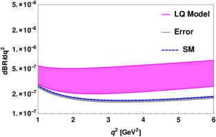
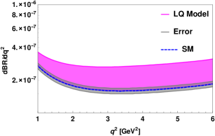
Figure 2: The differential branching ratios of $\bar{B}\to\bar{K}^{*}e^{+}e^{-}$ (left panel) and $\bar{B}\to\bar{K}^{*}\mu^{+}\mu^{-}$ (right panel) processes with respect to the $q^{2}$ in the vector LQ model. Here the magenta bands represent the LQ contributions and the dotted lines are for the SM. The theoretical uncertainties arising due to the SM input parameters are shown as grey bands.

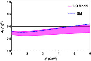
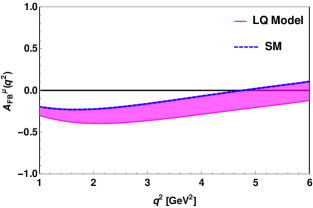
Figure 3: The $q^{2}$ variations of the forward-backward asymmetries of $\bar{B}\to\bar{K}^{*}e^{+}e^{-}$ (left panel) and $\bar{B}\to\bar{K}^{*}\mu^{+}\mu^{-}$ (right panel) processes in the vector LQ model.

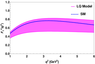
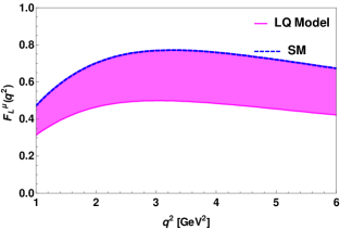
Figure 4: The $q^{2}$ variations of the longitudinal polarizations of $\bar{B}\to\bar{K}^{*}e^{+}e^{-}$ (left panel) and $\bar{B}\to\bar{K}^{*}\mu^{+}\mu^{-}$ (right panel) processes in the vector LQ model.

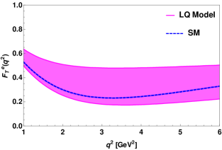
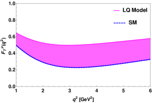
Figure 5: The $q^{2}$ variations of the transverse polarizations of $\bar{B}\to\bar{K}^{*}e^{+}e^{-}$ (left panel) and $\bar{B}\to\bar{K}^{*}\mu^{+}\mu^{-}$ (right panel) processes in the vector LQ model.

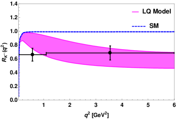
Figure 6: The variations of $R_{K^{*}}(q^{2})$ in the $q^{2}\in[0.045,6.0]~{}{\rm GeV}^{2}$ regions in the vector LQ model.

Table 4: The predicted integrated values of the branching ratio, forward-backward asymmetry and lepton polarization asymmetry with respect to low $q^{2}$ for the $\bar{B}\rightarrow\bar{K}^{*}l^{+}l^{-}$ processes in the SM and the vector LQ model.

Observables	SM prediction	Values in LQ model
BR($\bar{B}\rightarrow\bar{K}^{*}e^{+}e^{-}$)	$(8.97\pm 0.49~{}({\rm CKM})\pm 0.23~{}({\rm form~{}factor}))\times 10^{-7}$	$(1.155\to 2.882)\times 10^{-6}$
$\langle A_{FB}^{e}\rangle$	$-0.084\pm 0.005$	$-(0.314\to 0.064)$
$\langle F_{L}^{e}\rangle$	$0.703\pm 0.042$	$0.5\to 0.76$
$\langle F_{T}^{e}\rangle$	$0.297\pm 0.018$	$0.24\to 0.5$
BR($\bar{B}\rightarrow\bar{K}^{*}\mu^{+}\mu^{-}$)	$(8.9\pm 0.48~{}({\rm CKM})\pm~{}0.22~{}({\rm form~{}factor}))\times 10^{-7}$	$(0.892\to 1.45)\times 10^{-6}$
$\langle A_{FB}^{\mu}\rangle$	$-0.082\pm 0.0049$	$-(0.28\to 0.083)$
$\langle F_{L}^{\mu}\rangle$	$0.71\pm 0.043$	$0.46\to 0.71$
$\langle F_{T}^{\mu}\rangle$	$0.29\pm 0.017$	$0.29\to 0.54$

Table 5: The predicted integrated values of the lepton non-universality $(R_{K^{*}})$ parameter in the LQ model.

Observables	SM prediction	Values in LQ model
$\langle R_{K^{*}}\rangle|_{q^{2}\in[0.045,1.1]}$	$0.913$	$0.65\to 0.9$
$\langle R_{K^{*}}\rangle|_{q^{2}\in[1.1,6.0]}$	$0.9926$	$0.5\to 0.73$

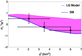
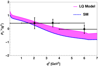
Figure 7: The plot in the left panel represent the $P_{5}^{\prime}(q^{2})$ observable for $\bar{B}\rightarrow\bar{K}^{*}e^{+}e^{-}$ precess in the vector LQ model. The corresponding plot for $\bar{B}\rightarrow\bar{K}^{*}\mu^{+}\mu^{-}$ process is shown in the right panel.

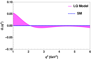
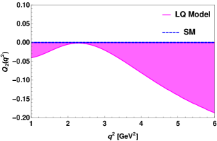
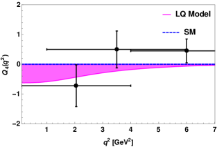
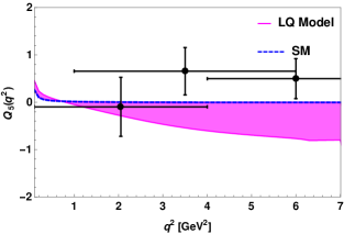
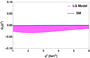
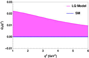
Figure 8: The plots in the left panel represent the $Q_{1}(q^{2})$ (top), $Q_{4}(q^{2})$ (middle) and $Q_{6}(q^{2})$ (bottom) observables in the vector LQ model. The $Q_{2}(q^{2})$ (top), $Q_{5}(q^{2})$ (middle) and $Q_{8}(q^{2})$ (bottom) plots are shown in the right panel.

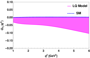
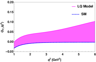
Figure 9: The $q^{2}$ variations of $Q_{F_{L}}(q^{2})$ (left panel) and $Q_{F_{T}}(q^{2})$ (right panel) observables in the vector LQ model.

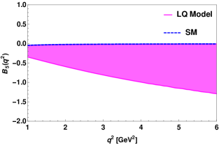
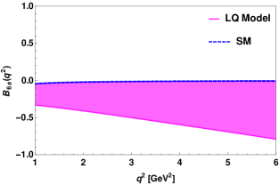
Figure 10: The $q^{2}$ variation of $B_{5}$ (left panel) and $B_{6s}$ (right panel) observables in the LQ model.

Table 6: The predicted values of the $P_{i}^{l^{(\prime)}}$ observables in the low $q^{2}$ $(q^{2}\in[1,6]~{}{\rm GeV}^{2})$ region for the $\bar{B}\rightarrow\bar{K}^{*}l^{+}l^{-}$ processes in the SM and the LQ model.

Observables	SM prediction	Values in LQ model
$\langle P_{1}^{e}\rangle$	$-0.045\pm 0.0027$	$-0.0448\to 0.15$
$\langle P_{2}^{e}\rangle$	$0.188\pm 0.011$	$0.19\to 0.415$
$\langle P_{3}^{e}\rangle$	$(-5.43\pm 0.326)\times 10^{-4}$	$-0.0143\to-5.43\times 10^{-4}$
$\langle P_{4}^{e\prime}\rangle$	$0.43\pm 0.0258$	$0.43\to 0.791$
$\langle P_{5}^{e\prime}\rangle$	$-0.226\pm 0.0136$	$-0.226\to 0.682$
$\langle P_{6}^{e\prime}\rangle$	$-0.0734\pm 0.0044$	$-0.0734\to-0.042$
$\langle P_{8}^{e\prime}\rangle$	$0.02678\pm 0.0016$	$-0.014\to 0.027$
$\langle P_{1}^{\mu}\rangle$	$-0.045\pm 0.0027$	$-0.0449\to 0.133$
$\langle P_{2}^{\mu}\rangle$	$0.185\pm 0.011$	$0.185\to 0.34$
$\langle P_{3}^{\mu}\rangle$	$(-5.41\pm 0.324)\times 10^{-4}$	$-0.013\to-5.41\times 10^{-4}$
$\langle P_{4}^{\mu\prime}\rangle$	$0.437\pm 0.026$	$0.44\to 0.536$
$\langle P_{5}^{\mu\prime}\rangle$	$-0.2318\pm 0.014$	$-0.231\to 0.166$
$\langle P_{6}^{\mu\prime}\rangle$	$-0.0738\pm 0.0044$	$-0.0676\to-0.074$
$\langle P_{8}^{\mu\prime}\rangle$	$0.02676\pm 0.001$	$1.164\times 10^{-3}\to 0.027$

After collecting all possible angular observables, we now move on for the numerical analysis. We have taken all the particle masses and the lifetime of $B$ meson from pdg for the numerical estimation. We consider the Wolfenstein parametrization with the values $A=0.811\pm 0.026$, $\lambda=0.22506\pm 0.00050$, $\bar{\rho}=0.124^{+0.019}_{-0.018}$, and $\bar{\eta}=0.356\pm 0.011$ pdg for the CKM matrix elements. The QCD form factors for the $\bar{B}\to\bar{K}^{*}l^{+}l^{-}$ processes in the low $q^{2}$ region are taken from kstar-formfactor-1 ; kstar-formfactor-2 . Now using the constraints on the LQ couplings as discussed in section III, we show in Fig. 2, the $q^{2}$ variation of the differential branching ratios of $\bar{B}\to\bar{K}^{*}e^{+}e^{-}$ (left panel) and $\bar{B}\to\bar{K}^{*}\mu^{+}\mu^{-}$ (right panel) processes in the $V^{1}(3,1,2/3)$ vector LQ model. In the figures, the blue dashed lines stand for the SM contributions and the magenta bands are due to the exchange of vector LQ. Here the grey bands represent the theoretical uncertainties, which arise due to the uncertainties associated with the SM input parameters, such as the CKM matrix elements pdg and the hadronic form factors kstar-formfactor-1 ; kstar-formfactor-2 . From these figures, one can see that there is certain difference between the new physics contributions to the branching fractions of $\bar{B}\to\bar{K}^{*}e^{+}e^{-}$ and $\bar{B}\to\bar{K}^{*}\mu^{+}\mu^{-}$ processes. The predicted numerical values of the branching ratios in the high recoil limit are presented in Table IV. In the SM, the forward-backward asymmetry parameters of the $\bar{B}\to\bar{K}^{*}l^{+}l^{-}$ processes have negative values in the low-$q^{2}$ region. However, the contribution of new Wilson coefficients ($C_{9,10}^{(\prime)}$ and $C_{S,P}^{(\prime)}$) to the SM due to the exchange of $(3,1,2/3)$ vector LQ may enhance the rate of forward-backward asymmetries and can shift the zero position of these asymmetries. The plots for the forward-backward asymmetry for the $\bar{B}\to\bar{K}^{*}e^{+}e^{-}$ (left panel) and $\bar{B}\to\bar{K}^{*}\mu^{+}\mu^{-}$ (right panel) processes are presented in Fig. 3 and the corresponding integrated values are given in Table IV. For both $B\to K^{*}e^{+}e^{-}(\mu^{+}\mu^{-})$ processes, we found that due to the LQ contributions the zero-crossing position of forward-backward asymmetry shifts to the right (i.e., towards high $q^{2}$ region) of its SM predicted value. The longitudinal and transverse polarisation components for the $\bar{B}\to\bar{K}^{*}e^{+}e^{-}$ (left panel) and $\bar{B}\to\bar{K}^{*}\mu^{+}\mu^{-}$ (right panel) processes both in the SM and in the LQ model are shown in the Fig. 4 and Fig. 5 respectively. The predicted values of $F_{L}^{l}(F_{T}^{l})$ asymmetry parameters in the LQ model are given in Table IV. In these observables also we found some difference between the SM values and the LQ contributions.

Table 7: The predicted values of the LFUV observables, ($Q_{F_{L,T}}$, $Q_{i}$ and $B_{5,6s}$) for the $B\rightarrow K^{*}l^{+}l^{-}$ processes in the SM and the LQ model.

Observables	SM prediction	Values in LQ model
$\langle Q_{1}\rangle$	$0$	$-0.017\to-0.0001$
$\langle Q_{2}\rangle$	$-0.003$	$-0.075\to-0.005$
$\langle Q_{3}\rangle$	$2\times 10^{-6}$	$2\times 10^{-6}\to 1.3\times 10^{3}$
$\langle Q_{4}\rangle$	$0.007$	$-0.255\to 0.01$
$\langle Q_{5}\rangle$	$-0.0058$	$-0.516\to-0.005$
$\langle Q_{6}\rangle$	$-4\times 10^{-4}$	$-0.032\to 5.8\times 10^{-3}$
$\langle Q_{8}\rangle$	$-2\times 10^{-5}$	$0\to 0.0152$
$\langle Q_{F_{L}}\rangle$	$0.07$	$-0.04\to 0.07$
$\langle Q_{F_{T}}\rangle$	$-0.007$	$-0.007\to 0.05$
$\langle B_{5}\rangle$	$1.25\times 10^{-3}$	$-0.85\to-1.27\times 10^{-3}$
$\langle B_{6s}\rangle$	$-0.027$	$-0.56\to-0.027$

In Fig. 6, we show the plot for the $R_{K^{*}}$ observable in the low $q^{2}$ regime in both the SM and vector LQ model. After the $q^{2}\sim 1.1~{}{\rm GeV^{2}}$ region, noticeable difference from the SM prediction is found due to the contribution of the vector LQ. From the figure it can be seen that the measured value of $R_{K^{*}}$ in the $q^{2}\in[1.1,6.0]~{}{\rm GeV}^{2}$ region can be described in the LQ model. The predicted values of $R_{K^{*}}$ in the LQ model for different bins are presented in Table V. We found that our predicted results in the vector LQ model are consistent with the corresponding measured experimental data. Thus, vector LQs could be considered as potential candidates to explain an possibly lepton flavour universality violation, should it be observed.

Fig. 7 shows the plots for the FFI observables, $P_{5}^{\prime l}$ with respect to $q^{2}$ in the large recoil limit. In this figure, the plot for $P_{5}^{\prime l}$ for the electron mode is presented in the left panel and the right panel contains the corresponding plot for $\bar{B}\to\bar{K}^{*}\mu^{+}\mu^{-}$ process. One can notice that, the LQ model encompasses the SM, but also exhibits potentially larger values of $P_{5}^{\prime l}$ observables. In Table VI, we have presented the corresponding numerical results. In addition to the $P_{5}^{\prime l}$ observable, we have also studied all the FFI observables, $P_{i}^{(\prime)l}$, where $i=1,2,3,4,6,8$ and the predicted numerical values are listed in Table VI.

The measurement of $R_{K^{*}}$ motivated us to look for other LFUV parameters in this process. Belle has recently measured the new LFUV $Q_{4}$ and $Q_{5}$ parameters Q4-Belle in the low $q^{2}$ region, $(1\leq q^{2}\leq 6)~{}{\rm GeV}^{2}$ with values

$$Q_{4}=0.498\pm 0.527\pm 0.166,~{}~{}~{}~{}~{}Q_{5}=0.656\pm 0.485\pm 0.103.$$ (29)

The $q^{2}$ variation of $Q_{i}$ parameters in the vector LQ model are presented Fig. 8. In this figure, the left panel contains the plots for the $Q_{1}(q^{2})$ (top), $Q_{4}(q^{2})$ (middle) and $Q_{6}(q^{2})$ (bottom) observables and the $Q_{2}(q^{2})$ (top), $Q_{5}(q^{2})$ (middle) and $Q_{8}(q^{2})$ (bottom) plots are given in the right panel. We observe that the additional contributions due to LQ has provided large shift in some of these observables from their SM values. In Fig. 9, we show the plots for $Q_{F_{L}}$ (left panel) and $Q_{F_{T}}$ (right panel) observables. We also show the plots for the $B_{5}$ (left panel) and $B_{6s}$ (right panel) parameters in Fig. 10. The numerical values of all these LFUV parameters are given in Table VII.

V $K_{L}\to\mu^{\mp}e^{\pm}$ process

The $V^{1}_{\mu}(3,1,2/3)$ vector LQ has also contribution to the lepton flavour violating $K_{L}\to\mu^{\mp}e^{\pm}$ decay process. The effective Hamiltonian for $K_{L}\to\mu^{-}e^{+}$ LFV decays in the $(3,1,2/3)$ leptoquark model is given by

$$\mathcal{H}_{\rm LQ} = C_{LL}\left(\bar{d}\gamma^{\mu}\left(1-\gamma_{5}\right)s\right)\left(\bar{\mu}\gamma_{\mu}\left(1-\gamma_{5}\right)e\right)+C_{RR}\left(\bar{d}\gamma^{\mu}\left(1+\gamma_{5}\right)s\right)\left(\bar{\mu}\gamma_{\mu}\left(1+\gamma_{5}\right)e\right)$$ (30)

$$+ C_{LR}\left(\bar{d}\left(1+\gamma_{5}\right)s\right)\left(\bar{\mu}\left(1-\gamma_{5}\right)e\right)+C_{RL}\left(\bar{d}\left(1-\gamma_{5}\right)s\right)\left(\bar{\mu}\left(1+\gamma_{5}\right)e\right),~{}~{}$$

where the $C_{LL},C_{RR},C_{LR}~{}{\rm and}~{}C_{RL}$ coefficients are given as

$$C_{LL}=\frac{(g_{L})_{de}(g_{L})_{s\mu}^{*}}{4M_{\rm LQ}^{2}},~{}~{}~{}~{}~{}~{}~{}~{}C_{RR}=\frac{(g_{R})_{de}(g_{R})_{s\mu}^{*}}{4M_{\rm LQ}^{2}},$$

$$C_{LR}=\frac{(g_{L})_{de}(g_{R})_{s\mu}^{*}}{2M_{\rm LQ}^{2}},~{}~{}~{}~{}~{}~{}~{}~{}~{}C_{RL}=\frac{(g_{R})_{de}(g_{L})_{s\mu}^{*}}{2M_{\rm LQ}^{2}},$$ (31)

and for $K_{L}\to\mu^{+}e^{-}$ process

$$\mathcal{H}_{\rm LQ} = D_{LL}\left(\bar{d}\gamma^{\mu}\left(1-\gamma_{5}\right)s\right)\left(\bar{e}\gamma_{\mu}\left(1-\gamma_{5}\right)\mu\right)+D_{RR}\left(\bar{d}\gamma^{\mu}\left(1+\gamma_{5}\right)s\right)\left(\bar{e}\gamma_{\mu}\left(1+\gamma_{5}\right)\mu\right)$$ (32)

$$+ D_{LR}\left(\bar{d}\left(1+\gamma_{5}\right)s\right)\left(\bar{e}\left(1-\gamma_{5}\right)\mu\right)+D_{RL}\left(\bar{d}\left(1-\gamma_{5}\right)s\right)\left(\bar{e}\left(1+\gamma_{5}\right)\mu\right),~{}~{}$$

where the $D_{LL},D_{RR},D_{LR}~{}{\rm and}~{}D_{RL}$ coefficients are given as

$$D_{LL}=\frac{(g_{L})_{d\mu}(g_{L})_{se}^{*}}{4M_{\rm LQ}^{2}},~{}~{}~{}~{}~{}~{}~{}~{}D_{RR}=\frac{(g_{R})_{d\mu}(g_{R})_{se}^{*}}{4M_{\rm LQ}^{2}},$$

$$D_{LR}=\frac{(g_{L})_{d\mu}(g_{R})_{se}^{*}}{2M_{\rm LQ}^{2}},~{}~{}~{}~{}~{}~{}~{}~{}~{}D_{RL}=\frac{(g_{R})_{d\mu}(g_{L})_{se}^{*}}{2M_{\rm LQ}^{2}}.$$ (33)

The LFV decay processes do not receive any contribution from the SM. In the literature KL-LQ ; KL-LFV , the LFV decay of kaon has been investigated in the leptoquark and other new physics models. The branching ratio of $K_{L}\to\mu^{-}e^{+}$ process in the leptoquark model is given by

$${\rm BR}(K_{L}\to\mu^{-}e^{+}) = \tau_{K_{L}}\frac{f_{K}^{2}}{8\pi M_{K}^{3}}\sqrt{\left(M_{K}^{2}-m_{\mu}^{2}-m_{e}^{2}\right)^{2}-4m_{\mu}^{2}m_{e}^{2}}\times$$

$$\Bigg{[}\Big{|}(C_{LL}+C_{RR})(m_{e}-m_{\mu})-(C_{LR}+C_{RL})\frac{M_{K}^{2}}{m_{s}+m_{d}}\Big{|}^{2}\left(M_{K}^{2}-(m_{\mu}+m_{e})^{2}\right)$$

$$+\Big{|}(C_{LL}-C_{RR})(m_{e}+m_{\mu})+(C_{LR}-C_{RL})\frac{M_{K}^{2}}{m_{s}+m_{d}}\Big{|}^{2}\left(M_{K}^{2}-(m_{\mu}-m_{e})^{2}\right)\Bigg{]}.$$

Similarly, the branching ratio of $K_{L}\to\mu^{+}e^{-}$ process can be obtained from Eqn. (V) by replacing the new coefficients $C_{ij}\to D_{ij}$, where ($i,j=L,R$). The branching ratio of $K_{L}\to\mu^{\mp}e^{\pm}$ process is simply the sum of the branching ratios of $K_{L}\to\mu^{-}e^{+}$ and $K_{L}\to\mu^{+}e^{-}$ processes. For the required LQ couplings, we use the couplings obtained from $K_{L}\to e^{+}e^{-}(\mu^{+}\mu^{-})$ process which are given in Table II and III as basis values and assumed that the LQ couplings between different generation of quark and lepton follow the simple scaling law, i.e., $(g_{L(R)})_{ij}=(m_{i}/m_{j})^{1/2}(g_{L(R)})_{ii}$ with $j>i$. We have taken this ansatz from the Ref. ansatz , which successfully explains the decay width of radiative LFV $\mu\to e\gamma$ decay. Now using this ansatz and the particle masses and life time of $K_{L}$ meson from pdg , the predicted branching ratios of $K_{L}\to\mu^{\mp}e^{\pm}$ process is given by

$${\rm BR}(K_{L}\to\mu^{\mp}e^{\pm}) = (1.78-3.564)\times 10^{-12}.$$ (35)

The corresponding experimental upper limit on branching ratio of $K_{L}\to\mu^{\mp}e^{\pm}$ process is given as pdg

$${\rm BR}(K_{L}\to\mu^{\mp}e^{\pm})~{}\textless~{}4.7\times 10^{-12}.$$ (36)

Our predicted branching ratios are within the experimental limit.

VI Conclusion

We have investigated the intriguing anomalies related with the rare semileptonic $\bar{B}\to\bar{K}^{*}l^{+}l^{-}$ decay processes in the context of a $(3,1,2/3)$ vector leptoquark model. We constrain the leptoquark couplings by using the experimental branching ratios of $B_{s}\to l^{+}l^{-}$, $K_{L}\to l^{+}l^{-}$ and $B_{s}\to\mu^{\mp}e^{\pm}$ processes. We then calculated the branching ratios, forward-backward asymmetries and the lepton polarization asymmetries of these processes. We found that there is appreciable difference between the SM and LQ model predictions. We have also calculated the form factor independent observables $P_{i}^{(\prime)}$, where $i=1,..,6,8$ in this model. We observed that vector leptoquark can also explain the $P_{5}^{\prime}$ anomalies very well.

We then looked into the lepton nonuniversality parameter $R_{K^{*}}$ of the $\bar{B}\to\bar{K}^{*}l^{+}l^{-}$ process in both the $q^{2}\in[0.045,1.1]~{}{\rm GeV}^{2}$ and $q^{2}\in[1.1,6.0]~{}{\rm GeV}^{2}$ regions and found that the $R_{K^{*}}$ anomaly could be explained in the vector leptoquark model. We have also investigated a few other lepton nonuniversality observables in order to verify violation of lepton universality in the $B$ sector. Thus, along with the $R_{K^{*}}$ observable, we also studied some LNU observables, such as $Q_{F_{L}}$, $Q_{F_{T}}$, $Q_{i}$ and $B_{5,6s}$ in the vector leptoquark model. We observed that in the presence of a vector leptoquark, all the observables have some differences from their SM results but in many cases the SM results are within the uncertainties of the LQ model. We have also computed the branching ratio of the lepton flavour violating $K_{L}\to\mu^{\mp}e^{\pm}$ process in the $(3,1,2/3)$ vector leptoquark, which is found to be within the experimental limit. The observation of these observables in the LHCb experiment may provide indirect hints for the possible existence of leptoquark.

Acknowledgments

We would like to thank Science and Engineering Research Board (SERB), Government of India for financial support through grant No. SB/S2/HEP-017/2013.

References

- (1) R. Aaij et al., [LHCb Collaboration], JHEP 08, 055 (2017) [arXiv:1705.05802].
- (2) R. Aaij et al., [LHCb Collaboration], Phys. Rev. Lett. 113, 151601 (2014) [arXiv:1406.6482].
- (3) R. Aaij et al., [LHCb Collaboration], JHEP 1307, 084 (2013) [arXiv:1305.2168].
- (4) R. Aaij et al., [LHCb Collaboration], Phys. Rev. Lett. 111, 191801 (2013) [arXiv:1308.1707].
- (5) R. Aaij et al., [LHCb Collaboration], JHEP 1406, 133 (2014) [arXiv:1403.8044].
- (6) C. Langenbruch on behalf of the LHCb collaboration, [arXiv: 1505.04160].
- (7) R. Aaij et al. [LHCb Collaboration], Phys. Rev. Lett. 115, 111803 (2015) Addendum: Phys. Rev. Lett. 115, 159901 (2015) [arXiv:1506.08614].
- (8) BaBar Collaboration, J. Lees et al., Phys. Rev. Lett. 109, 101802 (2012) [arXiv:1205.5442]; BaBar Collaboration, J. Lees et al., Phys. Rev. D 88, 072012 (2013) [arXiv:1303.0571]; Belle Collaboration, M. Huschle et al., Phys. Rev. D 92, 072014 (2015) [arXiv:1507.03233]; Belle Collaboration, A. Abdesselam et al., [arXiv:1603.06711].
-
(9)
Heavy Flavour Averaging Group,
http://www.slac.stanford.edu/xorg/hfag/semi/winter16/
winter16_dtaunu.html. - (10) C. Bobeth, G. Hiller, G. Piranishvili, JHEP 12, 040 (2007) [arXiv:0709.4174].
- (11) B. Capdevila, A. Crivellin, S. Descotes-Genon, J. Matias, and J. Virto, JHEP 1801, 093 (2018) [arXiv:1704.05340].
- (12) H. Na et al., Phys. Rev. D 92, 054410 (2015) [arXiv:1505.03925].
- (13) S.Fajfer, J.F.Kamenik, and I.Nisandzic, Phys. Rev. D 85, 094025 (2012) [arXiv:1203.2654]; S. Fajfer, J. F. Kamenik, I. Nisandzic and J. Zupan, Phys. Rev. Lett. 109, 161801 (2012) [arXiv:1206.1872].
- (14) S. Wehle et al. [Belle Collaboration], Phys. Rev. Lett. 118, 111801 (2017) [arXiv:1612.05014].
- (15) G. D’Amico, M. Nardecchia, P. Panci, F. Sannino, A. Strumia, R. Torre, and A. Urbano, JHEP 09, 010 (2017) [arXiv:1704.05438]; G. Hiller, I. Nisandzic, Phys. Rev. D 96, 035003 (2017) [arXiv:1704.05444]; L.-S. Geng, B. Grinstein, S. Jger, J. M. Camalich, X.-L. Ren, and R.-X. Shi, Phys. Rev. D 96, 093006 (2017) [arXiv:1704.05446]; M. Ciuchini, A. M. Coutinho, M. Fedele, E. Franco, A. Paul, L. Silvestrini, and M. Valli, Eur. Phys. J. C 77, 688 (2017) [arXiv:1704.05447]; A. Celis, J. Fuentes-Martin, A. Vicente, and J. Virto, Phys. Rev. D 96, 035026 (2017) [arXiv:1704.05672]; D. Becirevic, and O. Sumensari, JHEP 1708, 104 (2017) [arXiv:1704.05835]; J. F. Kamenik, Y. Soreq, and J. Zupan, Phys. Rev. D 97, 035002 (2018) [arXiv:1704.06005]; F. Sala, and D. M. Straub, Phys. Lett. B 774, 205 (2017) [arXiv:1704.06188]; S. D. Chiara, A. Fowlie, S. Fraser, C. Marzo, L. Marzola, M. Raidal, and C. Spethmann, Nucl. Phys. B 923, 245 (2017) [arXiv:1704.06200]; D. Ghosh, [arXiv:1704.06240]; W. Altmannshofer, P. S. B. Dev, and A. Soni, Phys. Rev. D 96, 095010 (2017) [arXiv:1704.06659]; A. K. Alok, B. Bhattacharya, A. Datta, D. Kumar, J. Kumar, and D. London, Phys. Rev. D 96, 095009 (2017) [arXiv:1704.07397]; F. Bishara, U. Haisch and P. F. Monni, Phys. Rev. D 96, 055002 (2017) [arXiv:1705.03465]; T. Hurth, F. Mahmoudi, D. M. Santos and S. Neshatpour, Phys. Rev. D 96, 095034 (2017) [arXiv:1705.06274]; A. Datta, J. Kumar, J. Liao and D. Marfatia, [arXiv:1705.08423]; D. Bardhan, P. Byakti and D. Ghosh, Phys. Lett. B 773, 505 (2017) [arXiv:1705.09305]; S. Neshatpour, V.G. Chobanova, T. Hurth, F. Mahmoudi and D. M. Santos, [arXiv:1705.10730]; S. Matsuzaki, K. Nishiwaki and R. Watanabe, JHEP 1708, 145 (2017) [arXiv:1706.01463]; C.-W. Chiang, X.-G. He, J. Tandean and X.-Bo Yuan, Phys. Rev. D 96, 115022 (2017) [arXiv:1706.02696]; J. Kawamura, S. Okawa and Y. Omura, Phys. Rev. D 96, 075041 (2017) [arXiv:1706.04344]; B. Chauhan, B. Kindra and A. Narang, [arXiv:1706.04598]; S. Khalil, [arXiv:1706.07337].
- (16) S. Sahoo and R. Mohanta, Phys. Rev. D 93, 034018 (2016) [arXiv:1507.02070];
- (17) B. Capdevila, S. Descotes-Genon, J. Matias and J. Virto, JHEP 1610, 075 (2016) [arXiv:1605.03156].
- (18) H. Georgi, and S. L. Glashow, Phys. Rev. Lett. 32, 438 (1974); H. Fritzsch and P. Minkowski, Ann. Phys. 93, 193 (1975); P. Langacker, Phys. Rep. 72, 185 (1981).
- (19) J. C. Pati, and A. Salam, Phys. Rev. D 10, 275 (1974).
- (20) J.C. Pati, and A. Salam, Phys. Rev. D 8, 1240(1973); Phys. Rev. Lett. 31, 661 (1973); O. Shenkar, Nucl. Phys. B 206, 253 (1982); O. Shenkar, Nucl. Phys. B 204, 375 (1982).
- (21) D. B. Kaplan, Nucl. Phys. B 365, 259 (1991).
- (22) B. Schrempp, and F. Shrempp, Phys. Lett. B 153, 101 (1985); B. Gripaios, JHEP 1002, 045 (2010) [arXiv:0910.1789].
- (23) R. Mohanta, Phys. Rev. D 89, 014020 (2014) [arXiv:1310.0713]; S. Sahoo and R. Mohanta, Phys. Rev. D 91, 094019 (2015) [arXiv:1501.05193].
- (24) S. Sahoo and R. Mohanta, New J. Phys. 18, 013032 (2016) [arXiv:1509.06248]; Phys. Rev. D 93, 114001 (2016) [arXiv:1512.04657]; New J.Phys. 18, 093051 (2016) [arXiv:1607.04449]; J.Phys. G 44, 035001 (2017) [arXiv:1612.02543]; Eur. Phys. J. C 77, 344 (2017) [arXiv:1705.02251]; S. Sahoo, R. Mohanta, and A. K. Giri, Phys. Rev. D 95, 035027 (2017) [arXiv:1609.04367].
- (25) M. Duraisamy, S. Sahoo, and R. Mohanta, Phys. Rev. D 95, 035022 (2017) [arXiv:1610.00902].
- (26) S. Davidson, D. C. Bailey and B. A. Campbell, Z. Phys. C 61, 613 (1994) [arXiv:hep-ph/9309310]; I. Dorsner, S. Fajfer, J. F. Kamenik, N. Kosnik, Phys. Lett. B 682, 67 (2009) [arXiv:0906.5585]; S. Fajfer, N. Kosnik, Phys. Rev. D 79, 017502 (2009) [arXiv:0810.4858]; R. Benbrik, M. Chabab, G. Faisel, [arXiv:1009.3886]; A. V. Povarov, A. D. Smirnov, [arXiv:1010.5707]; J. P Saha, B. Misra and A. Kundu, Phys. Rev. D 81, 095011 (2010) [arXiv:1003.1384]; I. Dorsner, J. Drobnak, S. Fajfer, J. F. Kamenik, N. Kosnik, JHEP 11, 002 (2011) [arXiv:1107.5393]; F. S. Queiroz, K. Sinha, A. Strumia, Phys. Rev. D 91, 035006 (2015) [arXiv:1409.6301]; B. Allanach, A. Alves, F. S. Queiroz, K. Sinha, A. Strumia, Phys. Rev. D 92, 055023 (2015) [arXiv:1501.03494]; Ivo de M. Varzielas, G. Hiller, JHEP 1506, 072 (2005) [arXiv:1503.01084]; I. Dorsner, S. Fajfer, A. Greljo, J. F. Kamenik, N. Kosnik, doi:10.1016/j.physrep.2016.06.001, [arXiv:1603.04993]; S. Fajfer, J. F. Kamenik, I. Nisandzic and J. Zupan, Phys. Rev. Lett. 109, 161801 (2012) [arXiv:1206.1872]; M. Freytsis, Z. Ligeti and J. T. Ruderman, Phys. Rev. D 92, 054018 (2015) [arXiv:1506.08896]; I. Dorsner, S. Fajfer, J. F. Kamenik and N. Kosnik, Phys. Lett. B 682, 67 (2009) [arXiv:0906.5585]; L. Calibbi, A. Crivellin, T. Ota, Phys. Rev. Lett. 115, 181801 (2015) [arXiv:1506.02661]; Xin-Q. Li, Ya-D. Yang, X. Zhang, [arXiv:1605.09308]; B. Dumont, K. Nishiwaki, R. Watanabe, Phys. Rev. D 94, 034001 (2016) [arXiv:1603.05248]; M. Bauer and M. Neubert, Phys. Rev. Lett. 116, 141802 (2016) [arXiv:1511.01900]; S. Fajfer, N. Kosnik, doi:10.1016/j.physletb.2016.02.018, [arXiv:1511.06024]; D. Becirevic, S. Fajfer, N. Kosnik, O. Sumensari, Phys. Rev. D 94, 115021 (2016) [arXiv:1608.08501].
- (27) N. Kosnik, Phys. Rev. D 86, 055004 (2012), [arXiv:1206.2970].
- (28) G. Kumar, Phys. Rev. D 94, 014022 (2016) [arXiv: 1603.00346].
- (29) A. J. Buras and M. Munz, Phys. Rev. D 52, 186 (1995); M. Misiak, Nucl. Phys. B 393, 23 (1993); ibid. 439, 461 (E) (1995).
- (30) Wei-Shu Hou, M. Kohda and F. Xu, Phys. Rev. D 90, 013002 (2014) [arXiv:1403.7410].
- (31) K. De Bruyn, R. Fleischer, R. Knegjens, P. Koppenburg, M. Merk, A. Pellegrino, and N. Tuning, Phys. Rev. Lett. 109, 041801 (2012); A. J. Buras, R. Fleischer, J. Girrbach and R. Knegjens, JHEP 1307, 77 (2013) [arXiv:1303.3820].
- (32) C. Bobeth, M. Gorbahn, T. Hermann, M. Misiak, E. Stamou, and M. Steinhauser, Phys. Rev. Lett. 112, 101801 (2014).
- (33) T. Aaltonen et al. (CDF Collaboration), Phys. Rev. Lett. 102, 201801 (2009).
- (34) LHCb, CMS Collaboration, V. Khachatryan et al., Nature 522, 68 (2015) [arXiv:1411.4413].
- (35) LHCb Collaboration, LHCb-CONF-2016-011, https://cds.cern.ch/record/2220757.
- (36) G. Buchalla and A. J. Buras, Nucl. Phys. B 412, 106 (1994) [arXiv:hep-ph/9308272].
- (37) M. Misiak and J. Urban, Phys. Lett. B 451, 161 (1999) [arXiv:hep-ph/9901278]; G. Buchalla and A. J. Buras, Nucl. Phys. B 548, 309 (1999) [arXiv:hep-ph/9901288].
- (38) G. Isdori and R. Unterdorfer, JHEP 0401, 009 (2004) [arXiv:hep-ph/0311084].
- (39) C. Patrignani et al. (Particle Data Group), Chin. Phys. C 40, 100001 (2016).
- (40) C. Bobeth, G. Hiller and G. Piranishivili, JHEP 07, 106 (2008) [arXiv:0805.2525].
- (41) U. Egede, T. Hurth, J. Matias, M. Ramon, W. Reece, JHEP 10, 056 (2010) [arXiv:1005.0571].
- (42) U. Egede, T. Hurth, J. Matias, M. Ramon, W. Reece, JHEP 11, 032 (2008) [arXiv:0807.2589].
- (43) F. Kr ̵̈uger, J. Matias, Phys. Rev. D 71, 094009 (2005) [arXiv:hep-ph/0502060].
- (44) F. Beaujean, C. Bobeth, D. van Dyk and C. Wacker, JHEP 08, 030 (2012) [arXiv:1205.1838].
- (45) J. Matias, F. Mescia, M. Ramon and J. Virto, JHEP 04, 104 (2012) [arXiv:1202.4266].
- (46) S. Descotes-Genon, J. Matias, M. Ramon, J. Virto, JHEP 01, 048 (2013) [arXiv:1207.2753].
- (47) M. Beneke, T. Feldmann and D. Seidel, Eur. Phys. J. C 41, 173 (2005) [arXiv:hep-ph/0412400].
- (48) P. Ball and R. Zwicky, Phys. Rev. D 71, 014029 (2005) [hep-ph/0412079].
- (49) A. Crivellin, G. D’Ambrosio, M. Hoferichter, L. C. Tunstall, Phys. Rev. D 93, 074038 (2016) [arXiv: 1601.00970].
- (50) B. Gripaios, M. Nardecchia, S. A. Renner, JHEP 1505, 006 (2015) [arXiv:1412.1791]; S. Davidson, G. Isidori, and S. Uhlig, Phys. Lett. B 663, 73 (2008) [arXiv:0711.3376]; M. Redi, JHEP 1309, 060 (2013) [arXiv:1306.1525].