Benefits from using mixed precision computations in the ELPA-AEO and ESSEX-II eigensolver projects

Abstract

We first briefly report on the status and recent achievements of the ELPA-AEO (Eigenvalue Solvers for Petaflop Applications – Algorithmic Extensions and Optimizations) and ESSEX II (Equipping Sparse Solvers for Exascale) projects. In both collaboratory efforts, scientists from the application areas, mathematicians, and computer scientists work together to develop and make available efficient highly parallel methods for the solution of eigenvalue problems. Then we focus on a topic addressed in both projects, the use of mixed precision computations to enhance efficiency. We give a more detailed description of our approaches for benefiting from either lower or higher precision in three selected contexts and of the results thus obtained.

1 Introduction

Eigenvalue computations are at the core of simulations in various application areas, including quantum physics and electronic structure computations. Being able to best utilize the capabilities of current and emerging high-end computing systems is essential for further improving such simulations with respect to space/time resolution or by including additional effects in the models. Given these needs, the ELPA-AEO and ESSEX-II projects contribute to the development and implementation of efficient highly parallel methods for eigenvalue problems, in different contexts.

Both projects are aimed at adding new features (concerning, e.g., performance and resilience) to previously developed methods and at providing additional functionality with new methods. Building on the results of the first ESSEX funding phase 2016-KreutzerThiesEtAl-PerformanceEngineeringAnd-LNCSE113:317-338 ; 2016-ThiesGalgonEtAl-TowardsAnExascale-LNCSE113:295-316 , ESSEX-II again focuses on iterative methods for very large eigenproblems arising, e.g., in quantum physics. ELPA-AEO’s main application area is electronic structure computation, and for these moderately sized eigenproblems direct methods are often superior. Such methods are available in the widely used ELPA library 2014-MarekBlumEtAl-TheELPALibrary-JPhysCondensMatter:213201 , which had originated in an earlier project 2011-AuckenthalerBlumEtAl-ParallelSolutionOf-ParallelComput:37:783-794 and is being improved further and extended with ELPA-AEO.

In Sections 2 and 3 we briefly report on the current state and on recent achievement in the two projects, with a focus on aspects that may be of particular interest to prospective users of the software or the underlying methods. In Section 4 we turn to computations involving different precisions. Looking at three examples from the two projects we describe how lower or higher precision is used to reduce the computing time.

2 The ELPA-AEO project

In the ELPA-AEO project, chemists, mathematicians and computer scientists from the Max Planck Computing and Data Facility in Garching, the Fritz Haber Institute of the Max Planck Society in Berlin, the Technical University of Munich, and the University of Wuppertal collaborate to provide highly scalable methods for solving moderately-sized ($n\lesssim 10^{6}$) Hermitian eigenvalue problems. Such problems arise, e.g., in electronic structure computations, and during the earlier ELPA project, efficient direct solvers for them had been developed and implemented in the ELPA library 2014-MarekBlumEtAl-TheELPALibrary-JPhysCondensMatter:213201 .

This library is widely used (see https://elpa.mpcdf.mpg.de/about for a description and pointers to the software), and it has been maintained and further improved continually since the first release in 2011. The ELPA library contains optimized routines for the steps in the direct solution of generalized Hermitian positive eigenproblems $AX=BX\Lambda$, that is, (i) the Cholesky decomposition $B=U^{H}U$, (ii) the transformation $A\mapsto\widetilde{A}=U^{-H}\!AU^{-1}$ to a standard eigenproblem $\widetilde{A}X=\widetilde{X}\Lambda$, (iii) the reduction of $\widetilde{A}$ to tridiagonal form, either in one step or via an intermediate banded matrix, (iv) a divide-and-conquer tridiagonal eigensolver, and (v) back-transformations for the eigenvectors corresponding to steps (iii) and (ii). A typical application scenario from electronic structure computations (“SCF cycle”) requires a sequence of a few dozens of eigenproblems $A^{(k)}X=BX\Lambda$ to be solved, where the matrix $B$ remains unchanged; see Section 4.3 for more details. ELPA is particularly efficient in this situation by explicitly building $U^{-1}$ for steps (ii) and (v).

ELPA-AEO is aimed at further improving the performance of computations that are already covered by ELPA routines and at providing new functionality. In the remainder of this section we highlight a few recent achievements that may be of particular interest to current and prospective users of the library.

An alternative approach for the transformation (ii) has been developed 2018-ManinLang-ReductionOfGeneralized-InPreparation , which is based on Cannon’s algorithm 1969-Cannon-ACellularComputer-PhD . The transformation is done with two matrix products: multiplication 1 computes the upper triangle $M_{u}$ of $M:=A\cdot U^{-1}$, then $M_{u}$ is transposed to obtain the lower triangle $M_{l}$ of $M^{H}=U^{-H}A$, and finally multiplication 2 computes the lower triangle of $M_{l}\cdot U^{-1}=\widetilde{A}$. Both routines assume that one dimension of the process grid is a multiple of the other. They make use of the triangular structure of their arguments to save on computation and communication. The timing data in Figure 1 show that the new implementations are highly competitive.

 

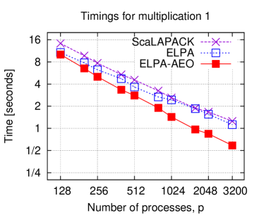
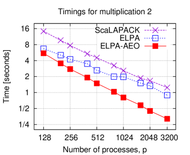
Figure 1: Timings for the two multiplications in the transformation $A\mapsto\widetilde{A}$ with routines from ScaLAPACK, current ELPA routines, and the new implementations. The runs were made on the HYDRA system at MPCDF in Garching with $20$ processes per node (two $10$-core Intel Ivy bridge processors running at 2.8 GHz) and double precision real matrices of size $n=30,000$. Process grids had aspect ratios $1:1$ or $1:2$; e.g., a $10\times 20$ grid was set up for $p=200$. With $p=3200$, the new codes run at $\approx 40$% of the nodes’ peak performance.

Recent ELPA releases provide extended facilities for performance tuning. The computational routines have an argument that can be used to guide the routines in selecting algorithmic paths (if there are different ways to proceed) and algorithmic parameters (such as block sizes) and to receive performance data from their execution. An easy-to-use autotuning facility allows setting such parameters in an automated way by screening the parameter space; see the code fragment in Figure 2 for an example. Note that the parameter set obtained with the coarse probing induced by ELPA_AUTOTUNE_FAST might be improved later on.

autotune_handle = elpa_autotune_setup( handle, ELPA_AUTOTUNE_FAST,                                    ELPA_AUTOTUNE_DOMAIN_REAL, &error ) ; for ( i = 0 ; i $<$ 20 ; i++ ) {      unfinished = elpa_autotune_step( handle, autotuning_handle ) ;      if ( unfinished == 0 )         printf( "ELPA autotuning finished in the %d th SCF step$\backslash$n", i ) ;      /* Solve EV problem */      elpa_eigenvectors( handle, a, ev, z, &error ) ; } elpa_autotune_best_set( handle, autotune_handle ) ; elpa_autotune_deallocate( autotune_handle ) ;

Figure 2: Using ELPA’s autotuning facility to adjust the algorithmic parameters during the solution of (at most) twenty eigenvalue problems in an SCF cycle, and saving them for later use.

In earlier releases, ELPA could be configured for single or double precision computations, but due to the naming conventions only one of the two versions could be linked to a calling program. Now, both precisions are accessible from one library, and mixing them may speed up some computations; see Section 4.3 for an example.

New functionality for addressing banded generalized eigenvalue problems will be added. An efficient algorithm for the transformation to a banded standard eigenvalue problem has been developed 2018-Lang-EfficientReductionOf-PREPRINT , and its parallelization is currently under way. This will complement the functions for solving banded standard eigenvalue problems that are already included in ELPA.

3 The ESSEX-II project

The ESSEX-II project is a collaborative effort of physicists, mathematicians and computer scientists from the Universities of Erlangen-Nuremberg, Greifswald, Tokyo, Tsukuba, and Wuppertal and from the German Aerospace Center in Cologne. It is aimed at developing exascale-enabled solvers for selected types of very large $(n\gg 10^{6}$) eigenproblems arising, e.g., in quantum physics; see the project’s homepage at https://blogs.fau.de/essex/ for more information, including pointers to publications and software.

ESSEX-II builds on results from the first ESSEX funding phase, in particular the Exascale enabled Sparse Solver Repository (ESSR), which provides a (block) Jacobi–Davidson method, the BEAST subspace iteration-based framework, and the Kernel Polynomial Method (KPM) and Chebyshev time propagation for determining few extremal eigenvalues, a bunch of interior eigenvalues, and information about the whole spectrum and dynamic properties, respectively.

Based on the versatile SELL-$C$-$\sigma$ format for sparse matrices 2014-KreutzerHagerEtAl-AUnifiedSparseMatrix-SIAMJSciComput:36:C401-C423 , the General, Hybrid, and Optimized Sparse Toolkit (GHOST) 2016-KreutzerThiesEtAl-GHOSTBuildingBlocks-IntJParallelProg:online contains optimized kernels for often-used operations such as sparse matrix times (multiple) vector products (optionally fused with other computations) and operations with block vectors, as well as a task manager, for CPUs, Intel Xeon Phi MICs and Nvidia GPUs and combinations of these. The Pipelined Hybrid-parallel Iterative Solver Toolkit (PHIST) 2016-ThiesGalgonEtAl-TowardsAnExascale-LNCSE113:295-316 provides the eigensolver algorithms with interfaces to GHOST and other “computational cores,” together with higher-level functionality, such as orthogonalization and linear solvers.

With ESSEX-II, the interoperability of these ESSR components will be further improved to yield a mature library, which will also have an extended range of applicability, including non-Hermitian and nonlinear eigenproblems. Again we highlight only a few recent achievements.

The Scalable Matrix Collection (ScaMaC) provides routines that simplify the generation of test matrices. The matrices can be chosen from several physical models, e.g., boson or fermion chains, and parameters allow adjusting sizes and physically motivated properties of the matrices. With $32$ processes, a distributed size $2.36$G matrix for a Hubbard model with $18$ sites and $9$ fermions can be set up in less than $10$ minutes.

The block Jacobi–Davidson solver has been extended to non-Hermitian and generalized eigenproblems. It can be run with arbitrary preconditioners, e.g., the AMG preconditioner ML 2018-SongWubsEtAl-NumericalBifurcationAnalysis-CommunNonlinearSciNumerSimul:60:145-164 , and employs a robust and fast block orthogonalization scheme that can make use of higher-precision computations; see Section 4.2 for more details.

The BEAST framework has been extended to seamlessly integrate three different approaches for spectral filtering in subspace iteration methods (polynomial filters, rational filters based on plain contour integration, and a moment-based technique) and to make use of their respective advantages with adaptive strategies. The BEAST framework also benefits from using different precisions; see Section 4.1.

At various places, measures for improving resilience have been included, based on verifying known properties of computed quantities and on checksums, combined with checkpoint–restart. To simplify incorporating the latter into numerical algorithms, the Checkpoint–Restart and Automatic Fault Tolerance (CRAFT) library has been developed 2017-ShahzadThiesEtAl-CRAFTALibrary-PREPRINT . Figure 3 illustrates its use within the BEAST framework. CRAFT can handle the GHOST and PHIST data types, as well as user-defined types. Checkpoints may be nested to accommodate, e.g., low-frequency high-volume together with high-frequency low-volume checkpointing in multilevel numerical algorithms, and the checkpoints can be written asynchronously to reduce overhead. By relying on the Scalable Checkpoint/Restart (SCR) and User-Level Failure Mitigation (ULFM-) MPI libraries, CRAFT also provides support for fast node-level checkpointing and for handling node failures.

// BEAST init (omitted) Checkpoint beast_checkpoint( "BEAST", comm ) ; beast_checkpoint->add( "eigenvectors", &X ) ; beast_checkpoint->add( "eigenvalues", &e ) ; ... // Some more beast_checkpoint->add( "control_variables", &state ) ; beast_checkpoint->commit() ; beast_checkpoint->restartIfNeeded( NULL ) ; // BEAST iterations while ( !state.abort_condition ) {      // Compute projector, etc. (omitted)      ...      beast_checkpoint->update() ;      beast_checkpoint->write() ; }

Figure 3: Using the CRAFT library to checkpoint the current eigenvector approximations X and other quantities in every iteration of the main loop.

4 Benefits of using a different precision

Doing computations in lower precision is attractive from a performance point of view because it reduces memory traffic in memory-bound code and, in compute-bound situations, allows more operations per second, due to vector instructions manipulating more elements at a time. However, the desired accuracy often cannot be reached in single precision and then only a part of the computations can be done in lower precision, or a correction is needed; cf., e.g., baboulin2009accelerating for the latter. In Subsection 4.1 we describe an approach for reducing overall runtimes of the BEAST framework by using lower-precision computations for early iterations.

Higher precision, on the other hand, is often a means to improve robustness. It is less known that higher precision can also be beneficial w.r.t. runtime. This is demonstrated in Subsection 4.2 in the context of orthogonalization.

In Section 4.3 we come back to using lower precision, from the perspective of an important application area: self-consistent field (SCF) cycles in electronic structure computations. Each iteration of such a cycle requires the solution of a generalized eigenproblem (GEP). After briefly introducing the context, we discuss how ELPA-AEO’s features can be used to steer the precision from the application code, targeting either the entire solution of a GEP or particular steps within its solution.

4.1 Changing precision in subspace iteration-based eigensolvers

The BEAST framework 2017-GalgonKraemerLang-ImprovingProjectionBased-NumerLinearAlgebraAppl:2017:e2124 ; 2016-ThiesGalgonEtAl-TowardsAnExascale-LNCSE113:295-316 is aimed at finding those eigenpairs $(\lambda,x)$ of a generalized interior eigenproblem $Ax=Bx\lambda$ ($A$ Hermitian, $B$ Hermitian positive definite) with $\lambda$ in a given search interval $I_{\lambda}=[\underline{\lambda},\overline{\lambda}]$, in particular for interior eigenvalues. It is based on subspace iteration with spectral filtering and Rayleigh–Ritz extraction, that is, a subspace $U$ containing an approximate basis for the desired eigenvectors is constructed from some initial vectors $Y$, then a Rayleigh–Ritz step is used to obtain the approximate eigenpairs. If the desired residual threshold is not yet reached, we iterate, using the approximate eigenvectors in our choice of $Y$ for the following iteration; cf. also Figure 5 below. The main distinguishing factor of the variants BEAST-P/-C/-M in our framework is the construction of the subspace $U$.

BEAST-P, which is only applicable for standard eigenproblems, implements a polynomial filter 2016-PieperKreutzerEtAl-HighPerformanceImplementation-JComputPhys:325:226-243 ; doi:10.1137/1.9781611970739 , using matrix–(block) vector products to apply a polynomial in $A$ to $Y$,

$$U=\sum\limits_{j=0}^{N}{\omega_{j}A^{j}Y}.$$

In both BEAST-C and BEAST-M, the filter is applied via quadrature approximations of contour integrals of the form

$$r(B^{-1}A)\approx\frac{1}{2\pi i}\int_{\Gamma}z^{k}(zB-A)^{-1}B\,\mathrm{d}z,$$

where $\Gamma$ is a contour in the complex plane enclosing the sought eigenvalues and no others. BEAST-C follows Polizzi’s FEAST algorithm polizzi2009density in computing

$$U=\sum_{j=1}^{N}w_{j}(z_{j}B-A)^{-1}BY$$

with suitable nodes $z_{j}$ and weights $w_{j}$. This requires $N$ linear solves for each iteration of the eigensolver, with an $n\times m$ block vector of right hand sides $Y$. BEAST-M realizes a specific Sakurai–Sugiura method sakurai2003projection , Sakurai–Sugiura Rayleigh–Ritz sakurai2007cirr . Here, the subspace is constructed as

$$U=\left[U_{0},...,U_{s-1}\right],\quad\mbox{where}\quad U_{k}=\sum_{j=1}^{N}w_{j}z_{j}^{k}(z_{j}B-A)^{-1}BY.$$

Thus, again $N$ linear solves must be performed as in BEAST-C, but since the overall subspace is computed as a combination of their solution, $Y$ needs only $(1/s)$th the desired number of columns of $U$, which can reduce the cost of the linear solves. It should be noted that a traditional Sakurai–Sugiura Rayleigh–Ritz implementation requires very few, or only one iteration, with a large overall subspace size. However, we consider it here within the context of a constrained subspace size, making it a truly iterative method.

We first consider the effect of starting with single precision and switching to double precision in later iterations. Since BEAST is designed to behave iteratively, we expect that this effect should be limited. Figure 4 shows BEAST-P’s progress (smallest residual of the current approximations in each iteration) in solving a standard eigenproblem $AX=X\Lambda$ for a size $3200$ topological insulator matrix $A$ from the ESSEX repository 2014-AlvermannBasermannEtAl-ESSEXEquippingSparse-ProcEuroPar2014-LNCS:577-588 and $I_{\lambda}=[-0.5,0.5]$, which contains $36$ eigenpairs. We see that the residuals for single precision data and computations are very close to those obtained with double precision, until we reach the single precision barrier. Continuing in single precision leads to stagnation. By contrast, if we switch to double precision data and computations sufficiently before the barrier, convergence proceeds as if the entire run was in double precision. Even a later switch need not have dramatic effects; we see that convergence, although stalled temporarily by the single precision barrier, proceeds at the same rate and possibly even slightly faster when switched two and four iterations “too late.” In the case of $10$ iterations in single precision (two past the ideal of $8$), the overall residual reached after $15$ total iterations is again close to that of the full double and ideal switch computations.

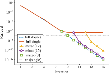
Figure 4: Smallest residual $\min_{i}\|Ax_{i}-\lambda_{i}x_{i}\|$ over BEAST-P iterations (with polynomial degree $50$) for computations done completely in double precision, completely in single precision, and with switching from single to double precision after iterations $12$, $10$, and $8$. The horizontal line indicates the single precision machine epsilon.

A switching strategy based on this observation is shown in Figure 5. In Figure 6 we report results for using this approach to solve the problem $AX=\Lambda X$ for a size $16$M graphene matrix from the ESSEX repository and $I_{\lambda}=\left[-0.0025,0.0025\right]$. The computation was done on the Emmy cluster at the University of Erlangen-Nuremberg, using 32 nodes, each with two Xeon 2660v2 chips. All methods computed an identical number of 318 eigenpairs in $I_{\lambda}$ to a tolerance of $10^{-10}$. BEAST-P exhibits a remarkable similarity in convergence rates between single and double precision before the switch threshold, and the mixed precision run was roughly $1.2$ times faster than using double precision throughout. In BEAST-C the rates are again similar; due to a few unconverged eigenpairs, the double precision computation required an additional iteration of the eigensolver for this problem, enabling a higher speedup $1.4$ for the mixed precision version. In BEAST-M, we observe some stagnation before the switch threshold, and an additional iteration was required in the mixed precision run. In this case, the mixed precision run was slower than pure double precision, with a “speedup” of $0.9$. Overall, the reduction in time from early iterations performed in single precision shows most clearly for BEAST-P. We note that the actual speed-up observed between single and double precision depends on both the hardware and software used; higher optimization of vectorized instructions or the use of accelerators such as GPUs could produce a more dramatic time difference.

Choose desired subspace size $m$ ($>\mbox{number of evals in $I_{\lambda}$}$) and initial vectors $Y$

while not converged do

       Construct subspace $U\leftarrow Y$ with BEAST-* scheme
Resize subspace based on $\mathrm{rank}(U)$
Solve reduced eigenproblem $A_{U}W=B_{U}W\Lambda$, where $A_{U}=U^{*}AU$, $B_{U}=U^{*}BU$
$X:=UW$
$Y:=BX$ (BEAST-P/-C) or $Y:=BXR$ (BEAST-M, with a random matrix $R$)
If single precision barrier has been reached, switch to double precision

end while

Figure 5: The mixed-precision BEAST framework. Computations are started in single precision and may be continued in double precision.

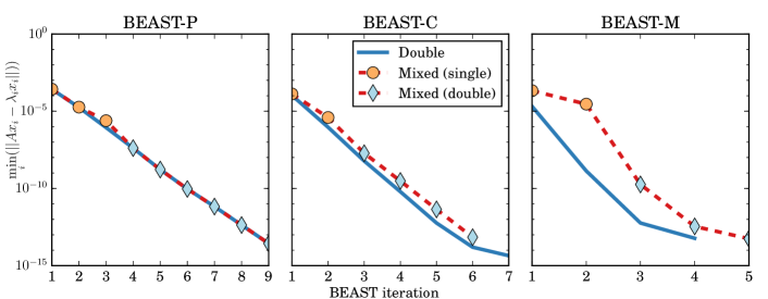
Figure 6: Smallest residual over BEAST iterations for runs done completely in double precision (solid lines) and for mixed precision runs (dashed lines; different markers for iterations done in single and double precision, respectively), with algorithmic parameters set as follows. Size of $U$: $1.5\times$ the estimated number of eigenvalues in the interval; polynomial degree of BEAST-P: $10,\!000$; $4$ Gauss-Legendre integration points for BEAST-C and $8$ for BEAST-M, which is more sensitive to a low number of nodes; STRUMPACK direct solver Rouet:2016:DPD:2956571.2930660 for the linear systems in BEAST-C and -M; threshold for the switch from single to double precision: $10^{-5}$ for BEAST-P and -C, and $10^{-4}$ for BEAST-M to prevent excessive stagnation.

The results indicate that initial iterations in single precision may have a limited effect on the overall convergence of the eigensolver if an appropriate switching point to double precision is chosen, thus allowing for a reduction in cost without sacrificing accuracy. We plan to combine this approach with relaxed stopping criteria for solving the linear systems in BEAST-C and -M iteratively; cf. also 2017-GalgonKraemerLang-ImprovingProjectionBased-NumerLinearAlgebraAppl:2017:e2124 ; doi:10.1002/nla.2188 for related work.

4.2 Using higher precision for robust and fast orthogonalization

In contrast to the standard Jacobi–Davidson method, which determines the sought eigenpairs one-by-one, the block Jacobi–Davison method in ESSEX 2015-RoehrigZoellnerThiesEtAl-IncreasingThePerformance-SIAMJSciComput:37:C697-C722 computes them by groups. Here we will consider only the real standard eigenvalue problem $Av_{i}=v_{i}\lambda_{i}$. Then one iteration contains the following two major steps:

1. Given $n_{b}$ current approximations $\tilde{\lambda}_{i}$ and $\tilde{v}_{i}$, $i=1,\ldots,n_{b}$, and a set of previously converged Schur vectors $W=(w_{1},\ldots,w_{k})$ ($k\geq 0$), use some steps of a (blocked) iterative linear solver for the correction equation

   $$(I-\tilde{W}\tilde{W}^{T})(A-\tilde{\lambda}_{i}I)(I-\tilde{W}\tilde{W}^{T})x_{i}\;=\;-r_{i},\quad i=1,\ldots,n_{b},$$

   where $r_{i}=A\tilde{v}_{i}-\tilde{v}_{i}\tilde{\lambda}_{i}$ are the current residuals and $\tilde{W}=(W\;|\;\tilde{v}_{1},\ldots,\tilde{v}_{n_{b}})$.

2. Obtain new directions $y_{1},\ldots,y_{n_{b}}$ by orthogonalizing the $x_{i}$ against $W$ and among themselves. (The $y_{i}$ are then used to update the $\tilde{v}_{i}$.)

The block method typically requires more operations than the non-blocked one and therefore has previously not been advocated, but in 2015-RoehrigZoellnerThiesEtAl-IncreasingThePerformance-SIAMJSciComput:37:C697-C722 it has been shown that this drawback can be more than outweighed by allowing the use of kernels that can be implemented to make best use of the capabilities of modern processors (in particular, sparse matrix times multiple vectors), such that the block method tends to run faster. In addition, it is more robust in the presence of multiple or tightly clustered eigenvalues.

In the following we focus on the orthogonalization in step 2. It is well known that if one first orthogonalizes the $x_{i}$ against $W$ (“phase I”) and then among themselves (“phase II”), the second phase can spoil the results of the first one; this also holds if we reverse the order of the phases. By contrast, a robust algorithm is obtained by iterating this process, alternating between the two phases and using a rank-revealing technique in phase II; see Hoemmen2010thesis ; Stewart2008bgs for a thorough discussion.

We follow this approach, using a plain projection $\tilde{Y}=(I-WW^{T})X$ for phase I and SVQB Stathopoulos2002 on $\tilde{Y}$ for phase II. We prefer SVQB over TSQR Demmel2012 because the bulk of computation may be done in a highly performant matrix–matrix multiplication for building the Gram matrix $M=\tilde{Y}^{T}\tilde{Y}$. This would also be true for CholQR Stathopoulos2002 , but SVQB is superior in the following sense.

Both methods orthogonalize $\tilde{Y}$ by determining a suitable matrix $Z\in\mathbb{R}^{n_{b}\times n_{b}}$ such that $Z^{T}MZ=I$, and setting $Y=\tilde{Y}Z$; this yields $Y^{T}Y=I$. For SVQB we take $Z=U\Lambda^{-1/2}$, where $M=U\Lambda U^{T}$ is an eigendecomposition of $M$, whereas a (possibly pivoted, partial) Cholesky decomposition $M=R^{T}R$ is used for setting $Z=R^{-1}$ in CholQR. In order to minimize amplification of rounding errors in the final multiplication $\tilde{Y}Z$, $Z$ should be as close as possible to the identity matrix, that is, we have to solve the optimization problem

$$\min_{Z\in\mathbb{R}^{n_{b}\times n_{b}},\,Z^{T}MZ=I}\|Z-I\|.$$

For the Frobenius norm, this is a special case of the orthogonal Procrustes problem analyzed by Schönemann in Schoenemann1966 , as it can be transformed to the following formulation:

$$\min_{\hat{Z}\in\mathbb{R}^{n_{b}\times n_{b}},\,\hat{Z}^{T}\hat{Z}=I}\|\bar{M}^{1/2}\hat{Z}-I\|_{F}.$$

As shown in Schoenemann1966 , a solution can be constructed as $\hat{Z}=UU^{T}$ with the eigendecomposition $M^{1/2}=UD^{1/2}U^{T}$ (in Schoenemann1966 a more general case is considered exploiting a singular value decomposition). So the choice $Z=M^{-1/2}\hat{Z}=UD^{-1/2}$, that is, the SVQB algorithm, is optimal in the sense discussed above. (For simplicity of the presentation we have assumed $M$ to be full-rank, thus symmetric positive definite. The argumentation also can be extended to the rank-deficient case.)

Our aim is to obtain a robust and fast overall orthogonalization method with fewer iterations by using extended precision computations; cf. ytdd14vecpar ; ytd15sisc for related ideas in the context of CholQR and communication-avoiding GMRES.

In contrast to ytdd14vecpar ; ytd15sisc , we use extended precision throughout the orthogonalization, including the orthogonalization against $W$ and the computation and decomposition of the Gram matrix. Our own kernels are based on the techniques described in Muller2010 for working with numbers represented by two doubles (DD). Some of the kernels take standard double precision data and return DD results, others also take DD data as inputs. They make use of AVX2, Intel’s advanced vector extensions, with FMA (fused multiply–add) operations; see (Muller2010, , Chapter 5). As proposed there, divisions and square roots are computed using the Newton–Raphson method.

Figure 4.2 shows the results of a single two-phase orthogonalization, without iteration, for synthetic test matrices with varying condition. If $X$ is ill-conditioned then TSQR does a much better job on $X$ than SVQB, but this does not carry over to orthogonality against $W$, and using DD kernels can improve both orthogonalities by at least two orders of magnitude.

Error in $W^{T}Y$

Error in $Y^{T}Y$

&

Figure 7: Accuracy after one iteration (phase I and phase II) for synthetic test matrices $W\in\mathbb{R}^{n\times k}$, $X\in\mathbb{R}^{n\times n_{b}}$, where $n=1000$, $k=20$, and $n_{b}=4$.

On modern architectures, even the performance of matrix–matrix multiplications such as $\tilde{V}^{T}\tilde{V}$ is memory-bound if the matrix $\tilde{V}\in\mathbb{R}^{n\times n_{b}}$ is only very few columns wide. Then the additional arithmetic operations required in the DD kernels come almost for free, and operations on small $n_{b}\times n_{b}$ matrices are cost negligible, even in extended precision. Figure 8 compares timings for the overall orthogonalization with a straight-forward implementation, one that uses kernel fusion (combining several basic operations to further reduce memory accesses; not discussed here), and one with fused DD kernels. It reveals that using DD routines can even reduce overall time because the higher accuracy achieved in each iteration can lead to a lower number of iterations to reach convergence.

Figure 8: Runtime “per vector” for overall orthogonalization of $X\in\mathbb{R}^{n\times n_{b}}$ against $W\in\mathbb{R}^{n\times k}$ and $X$ (phases I and II, iterated until convergence at $\epsilon=10^{-10}$) on an Intel Haswell workstation. $\kappa(X)=10^{-6}$, $\kappa(X,W)=10^{-12}$, $n=8\cdot 10^{6}$, $k$ and $n_{b}$ are indicated on the horizontal axis.

This technique can be useful for any algorithm that requires orthogonalizing a set $X$ of vectors with respect to themselves and to another set $W$ of (already orthonormal) vectors. It also extends to $B$-inner products, which is important, e.g., when solving generalized eigenvalue problems.

4.3 Mixed precision in SCF cycles with ELPA-AEO

The solution of the quantum-mechanical electronic-structure problem is at the basis of studies in computational chemistry, solid state physics, and materials science. In density-functional theory (DFT), the most wide-spread electronic-structure formalism, this implies finding the electronic density $n(\vec{r})$ that minimizes ($E_{0}=\min E[n(\vec{r})]$) the convex total-energy functional $E[n(\vec{r})]$ under the constraint that the number of electrons, $N=\int\mathrm{d}\vec{r}\,n(\vec{r})$, is conserved. Here, the set of $3M$ nuclear coordinates $\{\vec{R}\}$ enters $E[n(\vec{r})]$ parametrically. Formally, this variational problem requires to find the stationary solution of the eigenvalue problem (EVP)

$$H[n(\vec{r})]\,\Psi(\vec{r})=\varepsilon\Psi(\vec{r})\quad\text{ with }\quad n(\vec{r})=\sum_{s=1}^{N}|\Psi_{s}(\vec{r})|^{2}$$ (1)

in Hilbert space by iteratively updating $n(\vec{r})$, which depends on the $N$ eigenstates $\Psi_{s}$ with the lowest eigenvalues $\varepsilon_{s}$. This so called self-consistent field (SCF) cycle runs until “self-consistency” is achieved, i.e., until the mean interaction field contained in $H[n_{k}(\vec{r})]$ and/or other quantities (see below) do not change substantially between iterations anymore. In each step of the SCF cycle, the integro-differential equation (1) has to be solved. In practice, this is done by algebraizing Eq. (1) via a basis set expansion $\Psi_{s}=\sum_{i}x_{si}\varphi_{i}(\vec{r})$ of the so called orbitals in terms of appropriately chosen basis functions $\varphi_{i}(\vec{r})$, e.g., plane waves, localized functions, etc. By this means, one obtains a generalized EVP

$$A[n(\vec{r})]\,x=\lambda Bx\;,$$

in which the Hamiltonian $A$ and the overlap matrix $B$ are defined as

$$A_{ij}[n(\vec{r})]=\int\mathrm{d}\vec{r}\,\varphi_{i}^{*}(\vec{r})\,H[n(\vec{r})]\,\varphi_{j}(\vec{r})\quad\text{ and }\quad B_{ij}=\int\mathrm{d}\vec{r}\,\varphi_{i}^{*}(\vec{r})\,\varphi_{j}(\vec{r})\;.$$ (2)

As becomes clear from Eq. (2), the size of the EVP is thus determined by the number $K$ of basis functions $\varphi_{i}(\vec{r})$ employed in the calculation. For efficient, atom-centered basis functions the ratio $N/K$ of required eigenstates to matrix dimension typically ranges between $10$ and $50$%, rendering a direct solver competitive.

One SCF cycle yields the total energy $E_{0}(\{\vec{R}\})$ for just one set of nuclear coordinates $\{\vec{R}\}$. Studying molecules and materials requires the exploration of the high dimensional potential-energy surface (PES) which is given by $E_{0}(\{\vec{R}\})$ as a function of $\{\vec{R}\}$, e.g., via molecular dynamics (MD), statistical (e.g. Monte Carlo) sampling, or minimization and saddle point search algorithms. Accordingly, a typical computational study requires thousands if not millions of SCF cycles (about $10$–$100$ SCF steps per cycle) to be performed in a single simulation. This large number of SCF steps makes it mandatory to investigate strategies to reduce the computational effort. Since only the final result of each converged SCF cycle is of physical relevance at all, the SCF procedure can be accelerated by using single precision (SP) routines instead of double precision (DP) ones in the appropriate eigensolver steps (cf. Section 2), as long as the final converged result is not altered up to the precision mandated by the problem at hand. The eigensolver steps discussed in this section are the Cholesky decomposition (i), the transformation to the standard eigenproblem (ii), and its standard diagonalization, which combines tridiagonalization (iii) and the tridiagonal eigensolver (iv), as defined in Section 2.

To showcase the importance of the readily available SP routines in ELPA-AEO, we have performed DFT calculations with the all-electron, numeric atomic orbitals based code FHI-aims Blum:2009fe , which supports both ELPA and ELPA-AEO through the ELSI package Yu:2018ih . For this purpose, we have run benchmark calculations for zirconia (ZrO₂) in its tetragonal polymorph, a wide band-gap insulator often employed as thermal insulator in aeronautic applications Carbogno:2014wa ; Carbogno:2017gc . Supercells containing between $M=6$ and $768$ atoms ($N=112$ and $14,\!336$ electrons) were investigated using the PBEsol exchange-correlation functional, “light” defaults for the numerical settings, and chemical species-specific “Tier 1” defaults for the basis functions $\varphi_{i}$. Accordingly, this translates to basis sets yielding matrix dimensions from $K=1,\!312$ to $70,\!848$ for the investigated systems. The finite $\vec{k}$-point grid required to sample reciprocal space to model such extended materials using periodic boundary conditions was chosen in such a way that the $\vec{k}$-point density is roughly constant (between $128$ and $216$ $\vec{k}$-points in the respective primitive Brillouin zone). As an example, Figure 9 shows the total time for one SCF step and the total time spent in solving the EVP with SP and DP as function of the system size. Here, SP is only used in the diagonalization (steps (iii) and (iv) introduced in Section 2). For larger system sizes (more than $10^{4}$ basis functions), the computational time spent in the calculation of $A[n(\vec{r})]$, which typically exhibits linear scaling with respect to $N$ in FHI-aims Havu:2009ug , becomes increasingly negligible compared to the EVP, which starts to dominate the computational time due to its cubic scaling. Switching from DP to SP thus allows for computational savings in the solution of the EVP on the order of $30$–$50$%. Even for medium system sizes ($M=96$ with $K=2,\!624$ basis functions) that are routinely addressed in DFT calculations Carbogno:2017gc this already translates into savings in total computational time of around $10$%, while savings of more than $20$% are observed for larger systems (up to over $40\%$ in Figure 12).

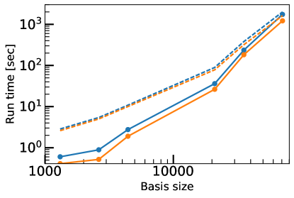
Figure 9: Total time for one SCF cycle (dashed lines) and total time spent in ELPA-AEO (solid lines) as function of the basis set size using SP (orange) and DP routines (blue) for zirconia (ZrO₂, $M$ from $6$ to $768$ atoms, $N$ from $112$ to $14,\!336$ electrons). The calculations were performed with $8$ Intel Xeon E5-2698v3 CPUs ($4$ nodes, $32$ cores/node) and $4$ GB of RAM per core.

However, SP routines cannot be exploited during the full SCF cycle: once a certain accuracy is reached, further SP SCF iterations do no longer approach convergence. This is demonstrated for ZrO₂ in Figure 10. In each SCF step, we monitor two properties that are typically used for determining the convergence of such calculations: (I) the change in charge density between two subsequent steps $k$ and $k+1$, $\Delta n=\int\mathrm{d}\vec{r}\,|n_{k}(\vec{r})-n_{k+1}(\vec{r})|$, and (II) the change in the sum of the $N$ lowest eigenvalues, $\Delta\varepsilon=\sum_{s=1}^{N}\varepsilon_{s}^{(k)}-\varepsilon_{s}^{(k+1)}$. For $M=162$ atoms, we observe that $\Delta n$ stalls at approximately $2.5\cdot 10^{-4}$ electrons after the $10$th SCF iteration for the calculation using SP. Similarly, $\Delta\varepsilon$ stalls at a value of $5\cdot 10^{-2}$ eV, showing a less regular behavior, both in SP and DP. This can be traced back to the fact that the total-energy functional is not variational with respect to the eigenvalues. As also shown in Figure 10 for $M=768$ atoms ($N=14,\!336$ electrons), the observed thresholds at which using SP no longer guarantees approaching convergence is, however, system and size dependent, since the respective quantities (energy, density, sum of eigenvalues, etc.) are extensive with system size, i.e., they scale linearly with the number of electrons, $N$. For these reasons, convergence criteria in DFT calculations are typically not chosen with respect to extensive quantities as the total energy, but with respect to intensive quantities, such as the total energy per atom. Hence the fraction of iterations for which SP routines can be used ($>30$%) are roughly independent of the system size, given that both the target quantity and its change, e.g., $n(\vec{r})$ and $\Delta n(\vec{r})$, are extensive with system size.

  

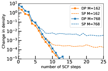
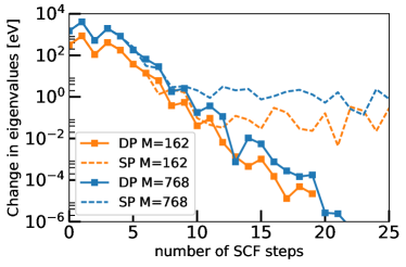
Figure 10: Change in density (left) and eigenvalues (right) as function of the number of SCF steps during a full SCF cycle when single-(squares) or double-precision (triangles) routines are used. Calculations were performed for zirconia ($M=162$ and $M=768$ atoms, $N=3,\!024$ and $14,\!336$ electrons, respectively, using the settings of Figure 9).

In general, not only the central steps (iii) and (iv) of solving the EVP (the diagonalization comprising the reduction to tridiagonal form and the tridiagonal eigensolver; cf. Section 2), but also the Cholesky decomposition (i) and the transformation to the standard eigenproblem (ii) offer the flexibility to choose between SP and DP. Even though the overlap-matrix $B$ remains constant during an SCF cycle for an atom-centered basis, the test calculations on an AB-stacked graphite system ($M=108$ atoms, PBE exchange-correlation functional, “tight” numerical defaults, “Tier 2” default basis set, $K=23,\!682$ basis functions, $N=648$ electrons) include the Cholesky decomposition in every iteration step in order to assess the impact of SP versus DP in step (i). Figure 11 illustrates that SP in (i) and (ii) does not noticeably change the convergence behavior of the extensive properties (change of total energy $\Delta E[n(\vec{r})]=E[n^{(k)}(\vec{r})]-E[n^{(k+1)}(\vec{r})]$, eigenvalues $\Delta\varepsilon$, and density $\Delta n$) during one SCF cycle and hence, full convergence is achieved in contrast to SP in the diagonalization (iii) and (iv). This is confirmed in the bottom right picture in Figure 11, where the forces on each atom, i.e., the gradients $\vec{F}_{I}=-\nabla_{\vec{R}_{I}}E_{0}(\{\vec{R}\})$ and their deviation from the full double precision values $|\vec{F}^{DP}_{I}-\vec{F}^{SP}_{I}|$ are shown. The force per atom, an intensive quantity, is typically monitored and required to reach a certain accuracy in calculations targeted at exploring $E_{0}(\{\vec{R}\})$. The bottom right plot in Figure 11 confirms that SP in the Cholesky decomposition (i) influences the results only marginally; SP transformation (ii) even yields numerically identical results (not shown on the logarithmic scale). By contrast, a SP diagonalization results in force deviations of up to $0.5$ meV/Å, which will still be sufficiently small for certain applications such as prescreening in PES exploration or statistical methods based on sampling by MD, when interpreting the error noise in the forces as acceptable thermal noise kuhne2007 . For the combination of SP throughout steps (i) to (iv), the convergence behavior and the force deviations are dominated by the performance of the eigensolver steps (iii) and (iv), and the convergence criteria for neither energy, eigenvalues, nor density are fulfilled. However, as discussed for Figures 9 and 10, resorting to a diagonalization (iii) and (iv) in SP during the initial SCF steps is computationally advantageous, but switching to DP is required in the final steps for full convergence.

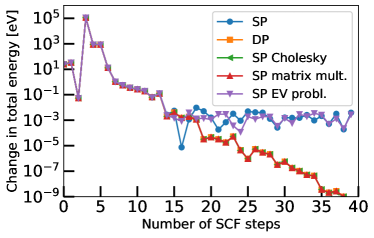
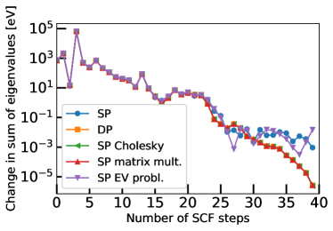
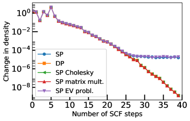
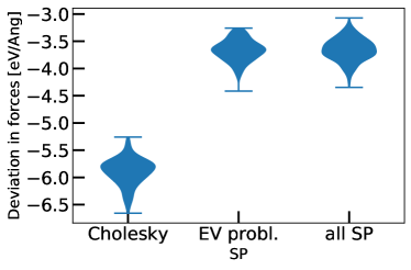
Figure 11: Convergence behavior of change in total energy (top left), change in sum of eigenvalues (top right), and change in density (bottom left) with the number of SCF iterations for AB-stacked graphite ($M=108$ atoms, $N=648$ electrons, $K=23,\!682$). SP in the Cholesky decomposition (step (i), green triangles) or the matrix multiplication (step (ii), red triangles) show convergence identical to full DP (orange squares) calculations and are essentially indistinguishable. SP in the diagonalization (steps (iii) and (iv), violet triangles) corrupts the convergence behavior. A combination of SP in steps (i) through (iv) (blue dots) does not reach convergence either. On the bottom right, the deviations in the forces per atom between SP and DP calculations are depicted for SP in different steps of the solution of the EVP.

Figure 12 shows that the discussed advantages of SP are preserved in massively parallelized computations. Here, we display calculations for a slab of silicon carbide, where a layer of graphene is adsorbed on the surface Nemec:2013jm . Compared to the 2013 ELPA code base, which presents a common usage scenario before the ELPA-AEO project, we observe a speed-up of $1.7$ for DP calculations. Another factor of $1.4$ is obtained when switching to SP, which would not have been possible with earlier releases of the library. The almost ideal strong scaling with respect to the number of cores is retained in SP calculations.

  

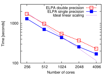
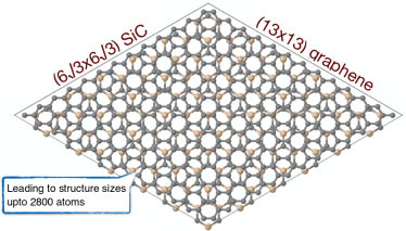
Figure 12: Time for solving the EVP for Zero-Layer Graphene ($M=1,\!742$, $65,\!346$ basis functions, LDA, $\Gamma$-point only) as function of the number of cores with DP (empty squares) and SP (filled squares). The calculations were performed with the IBM iDataPlex HPC system HYDRA using $2.6$ GHz Intel Sandy Bridge EP nodes with $16$ cores per node.

5 Concluding remarks

The ESSEX-II and ELPA-AEO projects are collaborative research efforts targeted at developing iterative solvers for very large scale eigenproblems (dimensions $\gg 1\mathrm{M}$) and direct solvers for smaller-scale eigenproblems (dimensions up to $1\mathrm{M}$), and at providing software for these methods. After briefly highlighting some recent progress in the two projects w.r.t. auto-tuning facilities, resilience, and added functionality, we have discussed several ways of using mixed precision for reducing the runtime.

In iterative schemes such as BEAST, single precision may be used in early iterations. This need not compromise the final accuracy if we switch to double precision at the right time. Even working in extended precision may speed up the execution if the extra precision leads to fewer iterations and is not too expensive, as seen with an iterative orthogonalization scheme for the block Jacobi–Davison method. Additional finer-grained control of the working precision, addressing just particular steps of the computations can also be beneficial; this has been demonstrated with electronic structure computations, where the precision for each step was chosen directly from the calling code.

Our results indicate that the users should be able to adapt the working precision, as well as algorithmic parameters, to their particular needs, together with heuristics for automatic selection. Work towards these goals will be continued in both projects.

References

- (1) Alvermann, A., Basermann, A., Fehske, H., Galgon, M., Hager, G., Kreutzer, M., Krämer, L., Lang, B., Pieper, A., Röhrig-Zöllner, M., Shahzad, F., Thies, J., Wellein, G.: ESSEX: Equipping sparse solvers for exascale. In: L. Lopes, et al. (eds.) Euro-Par 2014: Parallel Processing Workshops, LNCS, vol. 8806, pp. 577–588. Springer (2014)
- (2) Auckenthaler, T., Blum, V., Bungartz, H.J., Huckle, T., Johanni, R., Krämer, L., Lang, B., Lederer, H., Willems, P.R.: Parallel solution of partial symmetric eigenvalue problems from electronic structure calculations. Parallel Comput. 37(12), 783–794 (2011)
- (3) Baboulin, M., Buttari, A., Dongarra, J., Kurzak, J., Langou, J., Langou, J., Luszczek, P., Tomov, S.: Accelerating scientific computations with mixed precision algorithms. Comput. Phys. Comm. 180(12), 2526–2533 (2009)
- (4) Blum, V., Gehrke, R., Hanke, F., Havu, P., Havu, V., Ren, X., Reuter, K., Scheffler, M.: Ab initio molecular simulations with numeric atom-centered orbitals. Comput. Phys. Comm. 180, 2175–2196 (2009)
- (5) Cannon, L.E.: A cellular computer to implement the Kalman filter algorithm. Ph.D. thesis, Montana State University, Bozeman, MT (1969)
- (6) Carbogno, C., Levi, C.G., Van de Walle, C.G., Scheffler, M.: Ferroelastic switching of doped zirconia: Modeling and understanding from first principles. Phys. Rev. B 90, 144109 (2014)
- (7) Carbogno, C., Ramprasad, R., Scheffler, M.: Ab Initio Green-Kubo approach for the thermal conductivity of solids. Phys. Rev. Lett. 118(17), 175901 (2017)
- (8) Demmel, J., Grigori, L., Hoemmen, M., Langou, J.: Communication-optimal parallel and sequential QR and LU factorizations. SIAM J. Sci. Comput. 34(1), A206–A239 (2012)
- (9) Galgon, M., Krämer, L., Lang, B.: Improving projection‐based eigensolvers via adaptive techniques. Numer. Linear Algebra Appl. 25(1), e2124 (2017)
- (10) Gavin, B., Polizzi, E.: Krylov eigenvalue strategy using the FEAST algorithm with inexact system solves. Numer. Linear Algebra Appl. p. e2188 (2018)
- (11) Havu, V., Blum, V., Havu, P., Scheffler, M.: Efficient integration for all-electron electronic structure calculation using numeric basis functions. J. Comput. Phys. 228(22), 8367–8379 (2009)
- (12) Hoemmen, M.: Communication-avoiding Krylov subspace methods. Ph.D. thesis, University of California, Berkeley (2010)
- (13) Kreutzer, M., Hager, G., Wellein, G., Fehske, H., Bishop, A.R.: A unified sparse matrix data format for efficient general sparse matrix-vector multiplication on modern processors with wide SIMD units. SIAM J. Sci. Comput. 36(5), C401–C423 (2014)
- (14) Kreutzer, M., Thies, J., Pieper, A., Alvermann, A., Galgon, M., Röhrig-Zöllner, M., Shahzad, F., Basermann, A., Bishop, A.R., Fehske, H., Hager, G., Lang, B., Wellein, G.: Performance engineering and energy efficiency of building blocks for large, sparse eigenvalue computations on heterogeneous supercomputers. In: H.J. Bungartz, P. Neumann, W.E. Nagel (eds.) Software for Exascale Computing – SPPEXA 2013–2015, LNCSE, vol. 113, pp. 317–338. Springer, Switzerland (2016)
- (15) Kreutzer, M., Thies, J., Röhrig-Zöllner, M., Pieper, A., Shahzad, F., Galgon, M., Basermann, A., Fehske, H., Hager, G., Wellein, G.: GHOST: Building blocks for high performance sparse linear algebra on heterogeneous systems. Int. J. Parallel Prog. 45(5), 1046–1072 (2016)
- (16) Kühne, T.D., Krack, M., Mohamed, F.R., Parrinello, M.: Efficient and accurate Car-Parrinello-like approach to Born-Oppenheimer molecular dynamics. Phys. Rev. Lett. 98(6), 066401 (2007)
- (17) Lang, B.: Efficient reduction of banded hpd generalized eigenvalue problems to standard form (2018). Submitted
- (18) Manin, V., Lang, B.: Reduction of generalized hpd eigenproblems using Cannon’s algorithm for matrix multiplication (2018). In preparation
- (19) Marek, A., Blum, V., Johanni, R., Havu, V., Lang, B., Auckenthaler, T., Heinecke, A., Bungartz, H.J., Lederer, H.: The ELPA library: Scalable parallel eigenvalue solutions for electronic structure theory and computational science. J. Phys.: Condens. Matter 26(21), 213201 (2014)
- (20) Muller, J.M., Brisebarre, N., de Dinechin, F., Jeannerod, C.P., Lefv́re, V., Melquiond, G., Revol, N., Stehlé, D., Torres, S.: Handbook of Floating-Point Arithmetic. Springer Science + Business Media (2010)
- (21) Nemec, L., Blum, V., Rinke, P., Scheffler, M.: Thermodynamic equilibrium conditions of graphene films on SiC. Phys. Rev. Lett. 111(6), 065502 (2013)
- (22) Pieper, A., Kreutzer, M., Alvermann, A., Galgon, M., Fehske, H., Hager, G., Lang, B., Wellein, G.: High-performance implementation of Chebyshev filter diagonalization for interior eigenvalue computations. J. Comput. Phys. 325, 226–243 (2016)
- (23) Polizzi, E.: Density-matrix-based algorithm for solving eigenvalue problems. Phys. Rev. B 79(11), 115112 (2009)
- (24) Röhrig-Zöllner, M., Thies, J., Kreutzer, M., Alvermann, A., Pieper, A., Basermann, A., Hager, G., Wellein, G., Fehske, H.: Increasing the performance of the Jacobi–Davidson method by blocking. SIAM J. Sci. Comput. 37(6), C697–C722 (2015)
- (25) Rouet, F.H., Li, X.S., Ghysels, P., Napov, A.: A distributed-memory package for dense hierarchically semi-separable matrix computations using randomization. ACM Trans. Math. Software 42(4), 27:1–27:35 (2016)
- (26) Saad, Y.: Numerical Methods for Large Eigenvalue Problems, 2nd edn. Society for Industrial and Applied Mathematics, Philadelphia, PA (2011)
- (27) Sakurai, T., Sugiura, H.: A projection method for generalized eigenvalue problems using numerical integration. J. Comput. Appl. Math. 159(1), 119–128 (2003)
- (28) Sakurai, T., Tadano, H.: CIRR: a Rayleigh–Ritz type method with contour integral for generalized eigenvalue problems. Hokkaido Math. J. 36, 745–757 (2007)
- (29) Schönemann, P.H.: A generalized solution of the orthogonal Procrustes problem. Psychometrika 31(1), 1–10 (1966)
- (30) Shahzad, F., Thies, J., Kreutzer, M., Zeiser, T., Hager, G., Wellein, G.: CRAFT: A library for easier application-level checkpoint/restart and automatic fault tolerance (2017). Submitted. Preprint: arXiv:1708.02030
- (31) Song, W., Wubs, F., Thies, J., Baars, S.: Numerical bifurcation analysis of a 3D turing-type reaction–diffusion model. Commun. Nonlinear Sci. Numer. Simul. 60, 145–164 (2018)
- (32) Stathopoulos, A., Wu, K.: A block orthogonalization procedure with constant synchronization requirements. SIAM J. Sci. Comput. 23(6), 2165–2182 (2002)
- (33) Stewart, G.W.: Block Gram–Schmidt orthogonalization. SIAM J. Sci. Comput. 31(1), 761–775 (2008)
- (34) Thies, J., Galgon, M., Shahzad, F., Alvermann, A., Kreutzer, M., Pieper, A., Röhrig-Zöllner, M., Basermann, A., Fehske, H., Hager, G., Lang, B., Wellein, G.: Towards an exascale enabled sparse solver repository. In: H.J. Bungartz, P. Neumann, W.E. Nagel (eds.) Software for Exascale Computing – SPPEXA 2013–2015, LNCSE, vol. 113, pp. 295–316. Springer, Switzerland (2016)
- (35) Yamazaki, I., Tomov, S., Dong, T., Dongarra, J.: Mixed-precision orthogonalization scheme and adaptive step size for improving the stability and performance of CA-GMRES on GPUs. In: M.J. Daydé, O. Marques, K. Nakajima (eds.) High Performance Computing for Computational Science – VECPAR 2014 – 11th International Conference, Eugene, OR, USA, June 30–July 3, 2014, Revised Selected Papers, Lecture Notes in Computer Science, vol. 8969, pp. 17–30. Springer (2014)
- (36) Yamazaki, I., Tomov, S., Dongarra, J.: Mixed-precision Cholesky QR factorization and its case studies on multicore CPU with multiple GPUs. SIAM J. Sci. Comput. 37(3), C307–C330 (2015)
- (37) Yu, V.W., Corsetti, F., García, A., Huhn, W.P., Jacquelin, M., Jia, W., Lange, B., Lin, L., Lu, J., Mi, W., Seifitokaldani, A., Vázquez-Mayagoitia, Á., Yang, C., Yang, H., Blum, V.: ELSI: A unified software interface for Kohn–Sham electronic structure solvers. Comput. Phys. Comm. 222, 267–285 (2018)