Similarity encoding for learning with dirty categorical variables

Abstract

For statistical learning, categorical variables in a table are usually considered as discrete entities and encoded separately to feature vectors, e.g., with one-hot encoding. “Dirty” non-curated data gives rise to categorical variables with a very high cardinality but redundancy: several categories reflect the same entity. In databases, this issue is typically solved with a deduplication step. We show that a simple approach that exposes the redundancy to the learning algorithm brings significant gains. We study a generalization of one-hot encoding, similarity encoding, that builds feature vectors from similarities across categories. We perform a thorough empirical validation on non-curated tables, a problem seldom studied in machine learning. Results on seven real-world datasets show that similarity encoding brings significant gains in prediction in comparison with known encoding methods for categories or strings, notably one-hot encoding and bag of character n-grams. We draw practical recommendations for encoding dirty categories: 3-gram similarity appears to be a good choice to capture morphological resemblance. For very high-cardinality, dimensionality reduction significantly reduces the computational cost with little loss in performance: random projections or choosing a subset of prototype categories still outperforms classic encoding approaches.

1 Introduction

Many statistical learning algorithms require as input a numerical feature matrix. When categorical variables are present in the data, feature engineering is needed to encode the different categories into a suitable feature vector. One-hot encoding is a simple and widely-used encoding method alkharusi2012categorical ; berry1998factorial ; cohen2013applied ; davis2010contrast ; pedhazur1973multiple ; myers2010research ; ogrady1988categorical . For example, a categorical variable having as categories {female, male, other} can be encoded respectively with 3-dimensional feature vectors: {[1, 0, 0], [0, 1, 0], [0, 0, 1]}. In the resulting vector space, each category is orthogonal and equidistant to the others, which agrees with classical intuitions about nominal categorical variables.

Non-curated categorical data often lead to larger cardinality of the categorical variable and give rise to several problems when using one-hot encoding. A first challenge is that the dataset may contain different morphological representations of the same category. For instance, for a categorical variable named company, it is not clear if ‘Pfizer International LLC’, ‘Pfizer Limited’, and ‘Pfizer Korea’ are different names for the same entity, but they are probably related. Here we build upon the intuition that these entities should be closer in the feature space than unrelated categories, e.g., ‘Sanofi Inc.’. In dirty data, errors such as typos can cause morphological variations of the categories. Without data cleaning, different string representations of the same category will lead to completely different encoded vectors. Another related challenge is that of encoding categories that do not appear in the training set. Finally, with high-cardinality categorical variables, one-hot encoding can become impracticable due the high-dimensional feature matrix it creates.

Beyond one-hot encoding, the statistical-learning literature has considered other categorical encoding methods duch2000symbolic ; grkabczewski2003transformations ; micci2001preprocessing ; shyu2005handling ; weinberger2009feature , but, in general, they do not consider the problem of encoding in the presence of errors, nor how to encode categories absent from the training set.

From a data-integration standpoint, dirty categories may be seen as a data cleaning problem, addressed, for instance, with entity resolution. Indeed, database-cleaning research has developed many approaches to curate categories pyle1999data ; rahm2000data . Tasks such as deduplication or record linkage strive to recognize different variants of the same entity. A classic approach to learning with dirty categories would be to apply them as a preprocessing step and then proceed with standard categorical encoding. Yet, for the specific case of supervised learning, such an approach is suboptimal for two reasons. First, the uncertainty on the entity merging is not exposed to the statistical model. Second, the statistical objective function used during learning is not used to guide the entity resolution. Merging entities is a difficult problem. We build from the assumption that it may not be necessary to solve it, and that simply exposing similarities is enough.

In this paper, we study prediction with high-cardinality categorical variables. We seek a simple feature-engineering approach to replace the widely used one-hot encoding method. The problem of dirty categories has not received much attention in the statistical-learning literature—though it is related to database cleaning research krishnan2016activeclean ; krishnan2017boostclean . To ground it in supervised-learning settings, we introduce benchmarks on seven real-world datasets that contain at least one textual categorical variable with a high cardinality. The goal of this paper is to stress the importance of adapting encoding schemes to dirty categories by showing that a simple scheme based on string similarities brings important practical gains. In Section 2 we describe the problem of dirty categorical data and its impact on encoding approaches. In Section 3, we describe in detail common encoding approaches for categorical variables, as well as related techniques in database cleaning—record linkage, deduplication—and in natural language processing (NLP). Then, we propose in Section 4 a softer version of one-hot encoding, based on string similarity measures. We call this generalization similarity encoding, as it encodes the morphological resemblance between categories. We also present dimensionality reduction approaches that decrease the run time of the statistical learning task. Finally, we show in Section 5 the results of a thorough empirical study to evaluate encoding methods on dirty categories. On average, similarity encoding with 3-gram distance is the method that has the best results in terms of prediction score, outperforming one-hot encoding even when applying strong dimensionality reduction.

2 Problem setting: non-standardized categorical variables

In a classical statistical data analysis problem, a categorical variable is typically defined as a variable with values—categories—of either a nominal or ordinal nature. For example, place of birth is a nominal categorical variable. Conversely, answers in the Likert scale to the question: ‘Do you agree with this statement: A child’s education is the responsability of parents, not the school system.’, compose an ordinal categorical variable in which the level of agreement is associated with a numerical value. In addition, given a prediction problem, variables can be either the target variable (also known as the dependent or response variable) or an explanatory variable (a feature or independent variable). In this work, we focus on the general problem of nominal categorical variables that are part of the feature set.

In controlled data-collection settings, categorical variables are standardized: the set of categories is finite and known a priori—independently from the data—and categories are mutually exclusive. Typical machine-learning benchmark datasets, as in UCI Machine Learning Repository, use standardized categories. For instance, in the Adult dataset the occupation of individuals is described with 14 predefined categories in both the training and testing set.

A dirty data problem.

With non-standardized categorical variables the set of possible categories is unknown before the data collection process. One example of such non-standardized categories can be found in the Open Payments dataset, which describes financial relationships between healthcare companies and physicians or teaching hospitals. One possible task is to predict the value of the binary variable status (whether the payment has been done under a research protocol or not) given the following variables: corporation name, amount, and dispute (whether the physician refused the payment in a second instance). A challenge with this dataset is that some categories are not standardized. For instance, Table 1 shows all categories of the variable company name with the word Pfizer in it for the year 2013.

Table 1: Entities containing the word Pfizer in the variable company name of the Open Payments dataset (year 2013).

Company name	Frequency
Pfizer Inc.	79,073
Pfizer Pharmaceuticals LLC	486
Pfizer International LLC	425
Pfizer Limited	13
Pfizer Corporation Hong Kong Limited	4
Pfizer Pharmaceuticals Korea Limited	3

This type of data poses a problem from the point of view of the statistical analysis because we do not know a priori, without external expert information, which of these categories refer to the exact same company or whether all of them have slight differences and hence should be considered as different entities. Also, we can observe that the frequency of the different categories varies by several orders of magnitude, which could imply that errors in the data collection process have been made, unintentionally or not.

Often, the cardinality of a dirty categorical variable grows with the number of samples in the dataset. Figure 1 shows the cardinality of the corresponding categorical variable as a function of the number of samples for each of the seven datasets that we analyze in this paper.

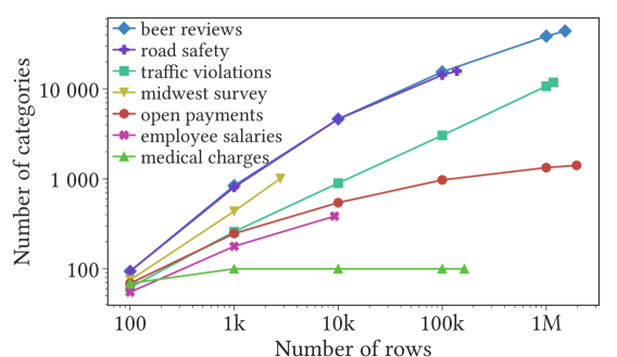
Figure 1: Evolution of the number of categories as a function of the number of samples. In six of our seven datasets, a higher number of samples implies a higher cardinality of the respective categorical variable. The dataset medical charges is the only one of this list that reaches its highest cardinality (100 categories) at around 1,000 samples.

Dirty categorical data can arise from a variety of mechanisms kim2003taxonomy :

• Typographical errors (e.g., proffesor instead of professor)

• Extraneous data (e.g., name and title, instead of just the name)

• Abbreviations (e.g., Dr. for doctor)

• Aliases (e.g., Ringo Starr instead Richard Starkey)

• Encoding formats (e.g., ASCII, EBCDIC, etc.)

• Uses of special characters (space, colon, dash, parenthesis, etc.)

• Concatenated hierarchical data (e.g., state-county-city vs. state-city)

A knowledge-engineering problem.

The presence of a large number of categories calls for representing the relationships between them. In knowledge engineering this is done via an ontology or a taxonomy. When the taxonomy is unknown, the problem is challenging. For example, in the medical charges dataset, ‘cervical spinal fusion’ and ‘spinal fusion except cervical’ are different categories, but both share the fact that they are a spinal fusion, hence they are not completely independent.

3 Related work and common practice

Most of the literature on encoding categorical variables relies on the idea that the set of categories is finite, known a priori, and composed of mutually exclusive elements cohen2013applied . Some studies have considered encoding high-cardinality categorical variables micci2001preprocessing ; guo2016entity , but not the problem of dirty data. Nevertheless, efforts on this issue have been made in other areas such as Natural Language Processing and Record Linkage, although they have not been applied to encode categorical variables. Below we summarize the main relevant approaches.

Notation:

we write sets of elements with capital curly fonts, as $\mathcal{X}$. Elements of a vector space are written in bold $\mathbf{x}$, and matrices in capital and bold $\mathbf{X}$. For a matrix $\mathbf{X}$, we denote by $x^{i}_{j}$ the entry on the $i$-th row and $j$-th column.

3.1 Formalism: concepts in relational databases and statistical learning

We first link our formulations to a database formalism, which relies on sets. A table is specified by its relational scheme $\mathcal{R}$: the set of $m$ attribute names $\{A_{j},j=1...m\}$, i.e., the column names maier1983theory . Each attribute name has a domain $\text{dom}(A_{j})=\mathcal{D}_{j}$. A table is defined as a relation $r$ on the scheme $\mathcal{R}$: a set of mappings (tuples) $\{t^{i}:\mathcal{R}\rightarrow\bigcup_{j=1}^{m}\mathcal{D}_{j},\;i=1...n\}$, where for each record (sample) $t^{i}\in r$, $t^{i}(A_{j})\in\mathcal{D}_{j},\;j=1...m$. If $A_{j}$ is a numerical attribute, then $\text{dom}(A_{j})=\mathcal{D}_{j}\subseteq\mathbb{R}$. If $A_{j}$ is a categorical attribute represented by strings, then $\mathcal{D}_{j}\subseteq\mathbb{S}$, where $\mathbb{S}$ is the set of finite-length strings. As a shorthand, we call $k_{j}=\text{card}(\mathcal{D}_{j})$ the cardinality of the variable.

As categorical entities are not numerical, they require an operation to define a feature matrix $\mathbf{X}$ from the relation $r$. Statistical or machine learning models that need vector data are applied after a categorical variable encoding, a feature map that consists of replacing the tuple elements $t^{i}(A_{j}),i=1...n$ by feature vectors:

$$\mathbf{x}_{j}^{i}\in\mathbb{R}^{p_{j}},p_{j}\geq 1.$$ (1)

Using the same notation in case of numerical attributes, we can define $\mathbf{x}_{j}^{i}=t^{i}(A_{j})\in\mathbb{R}^{p_{j}},p_{j}=1$ and write the feature matrix $\mathbf{X}$ as:

$$\mathbf{X}=\left[\begin{array}[]{*5{c}}\mathbf{x}_{1}^{1}&\ldots&\mathbf{x}_{m}^{1}\\ \vdots&\ddots&\vdots\\ \mathbf{x}_{1}^{n}&\ldots&\mathbf{x}_{m}^{n}\end{array}\right]\in\mathbb{R}^{n\times p},p=\sum_{j=1}^{m}p_{j}$$ (2)

In standard supervised-learning settings, the observations, represented by the feature matrix $\mathbf{X}$, are associated with a target vector $\mathbf{y}\in\mathbb{R}^{n}$ to predict.

We now review classical encoding methods. For simplicity of exposition, in the rest of the section we will consider only a single categorical variable $A$, omitting the column index $j$ from the previous definitions.

One-hot encoding.

Let $A$ be a categorical variable with cardinality $k\geq 2$ such that $\text{dom}(A)=\{d_{\ell},1<\ell\leq k\}$ and $t^{i}(A)=d^{i}$. The one-hot encoding method sets each feature vector as:

$$\mathbf{x}^{i}=\left[\mathbf{1}_{\{d_{1}\}}(d^{i}),\;\;\mathbf{1}_{\{d_{2}\}}(d^{i}),\;\;...\;,\;\;\mathbf{1}_{\{d_{k}\}}(d^{i})\right]\;\in\mathbb{R}^{k}$$ (3)

where $\mathbf{1}_{\{d_{\ell}\}}(\cdot)$ is the indicator function over the singleton $\{d_{\ell}\}$. Several variants of the one-hot encoding have been proposed, but in a linear regression, all perform equally in terms of $R^{2}$ score (see Cohen cohen2013applied for details).

The one-hot encoding method is intended to be used when categories are mutually exclusive cohen2013applied , which is not necessarily true of dirty data (e.g., misspelled variables should be interpreted as overlapping categories).

Another drawback of this method is that it provides no heuristics to assign a code vector to new categories that appear in the testing set but have not been encoded on the training set. Given the previous definition, the zero vector will be assigned to any new category in the testing set, which creates collisions if more that one new category is introduced.

Finally, high-cardinality categorical variables greatly increase the dimensionality of the feature matrix, which increases its computational cost. Dimensionality reduction on the one-hot encoding vector tackles this problem (see Subsection 4.2), with the risk of loosing information.

Hash encoding.

A solution to reduce the dimensionality of the data is to use the hashing trick weinberger2009feature . Instead of assigning a different unit vector to each category, as one-hot encoding does, one could define a hash function to designate a feature vector on a reduced vector space. This method does not consider the problem of dirty data either, because it assigns hash values that are independent of the morphological similarity between categories.

Encoding using target statistics.

The target encoding method micci2001preprocessing , is a variation of the VDM (value difference metric) continuousification scheme duch2000symbolic , in which each category is encoded given the effect it has on the target variable $\mathbf{y}$. The method considers that categorical variables can contain rare categories. Hence it represents each category by the probability of $\mathbf{y}$ conditional on this category. In addition, it takes an empirical Bayes approach to shrink the estimate. Thus, for a binary classification task:

$$\mathbf{x}^{i}=\lambda(n^{i})\,\mathbb{E}_{\ell}\bigl{[}\mathbf{y}^{\ell}|d^{\ell}=d^{i}\bigr{]}+\bigl{(}1-\lambda(n^{i})\bigr{)}\,\mathbb{E}_{\ell}\bigl{[}\mathbf{y}^{\ell}\bigr{]}\;\;\in\mathbb{R}$$ (4)

where $n^{i}$ is the frequency of the category $d^{i}$ and $\lambda(n^{i})\in[0,1]$ is a weight such that its derivative with respect to $n^{i}$ is positive, e.g., $\lambda(n^{i})=(\frac{n^{i}}{n^{i}+m},m>0$ micci2001preprocessing ). Note that the obtained feature vector is in this case one-dimensional.

Another related approach is the MDV continuousification scheme grkabczewski2003transformations , which encodes a category $d^{i}$ by its expected value on each target $c_{k}$, $\mathbb{E}_{\ell}\bigl{[}d^{\ell}=d^{i}|\mathbf{y}^{\ell}=c_{k}\bigr{]}$ instead of $\mathbb{E}_{\ell}\bigl{[}\mathbf{y}^{\ell}|d^{\ell}=d^{i}\bigr{]}$ used in the VDM. In the case of a classification problem, $c_{k}$ belongs to the set of possible classes for the target variable. However, in a dirty dataset, as with spelling mistakes, some categories can appear only once, undermining the meaning of their marginal link to $\mathbf{y}$.

Clustering.

To tackle the problem of high dimensionality for high-cardinality categorical variables, one approach is to perform a clustering of the categories and generate indicator variables with respect to the clusters. If $A$ is a categorical variable with domain $\mathcal{D}$ and cardinality $k$, we can partition the set $\mathcal{D}$ into $c\ll k$ clusters $\mathcal{D}_{1}...\mathcal{D}_{c}$; hence the feature vector associated to this variable is:

$$\mathbf{x}_{j}^{i}=\left[\mathbf{1}_{\mathcal{D}_{1}}(d^{i}),\mathbf{1}_{\mathcal{D}_{2}}(d^{i}),...,\mathbf{1}_{\mathcal{D}_{c}}(d^{i})\right]$$ (5)

To build clusters, Micci-Barreca micci2001preprocessing proposes grouping categories with similar target statistics, typically using hierarchical clustering.

Embedding with neural networks.

Guo guo2016entity proposes an encoding method based on neural networks. It is inspired by NLP methods that perform word embedding based on textual context mikolov2013efficient (see Subsection 3.2). In tabular data, the equivalent to this context is given by the values of the other columns, categorical or not. The approach is simply a standard neural network, trained to link the table $\mathcal{R}$ to the target $\mathbf{y}$ with standard supervised-learning architectures and loss and as inputs the table with categorical columns one-hot encoded. Yet, Guo guo2016entity uses as a first hidden layer a bottleneck for each categorical variable. The corresponding intermediate representation, learned by the network, gives a vector embedding of the categories in a reduced dimensionality. This approach is interesting as it guides the encoding in a supervised way. Yet, it entails the computational and architecture-selection costs of deep learning. Additionally, it is still based on an initial one-hot encoding which is susceptible to dirty categories.

Bag of n-grams.

One way to represent morphological variation of strings is to build a vector containing the count of all possible n-grams of consecutive characters (or words). This method is straightforward and naturally creates vectorial representations where similar strings are close to each other. In this work we consider n-grams of characters to capture the morphology of short strings.

3.2 Related approaches in natural language processing

Stemming or lemmatizing.

Stemming and lemmatizing are text preprocessing techniques that strive to extract a common root from different variants of a word lovins1968development ; hull1996stemming . For instance, ‘standardization’, ‘standards’, and ‘standard’ could all be reduced to ‘standard’. These techniques are based on a set of rules, crafted to the specificities of a language. Their drawbacks are that they may not be suited to a specific domain, such as medical practice, and are costly to develop. Some recent developments in NLP avoid stemming by working directly at the character level bojanowski2016enriching .

Word embeddings.

Capturing the idea that some categories are closer than others, such as ‘cervical spinal fusion’ being closer to ‘spinal fusion except cervical’ than to ‘renal failure’ in the medical charges dataset can be seen as a problem of learning semantics. Statistical approaches to semantics stem from low-rank data reductions of word occurrences: the original LSA (latent semantic analysis) landauer1998introduction is a PCA of the word occurrence matrix in documents; word2vec mikolov2013efficient can be seen as a matrix factorization on a matrix of word occurrence in local windows; and fastText bojanowski2016enriching , a state-of-the-art approach for supervised learning on text, is based on a low-rank representation of text.

However, these semantics-capturing embeddings for words cannot readily be used for categorical columns of a table. Indeed, tabular data seldom contain enough samples and enough context to train modern semantic approaches. Pretrained embeddings would not work for entries drawn from a given specialized domain, such as company names or medical vocabulary. Business or application-specific tables require domain-specific semantics.

3.3 Related approaches in database cleaning

Similarity queries.

To cater for different ways information might appear, databases use queries with inexact matching. Queries using textual similarity help integration of heterogeneous databases without common domains cohen1998integration .

Deduplication, record linkage, or fuzzy matching.

In databases, deduplication or record linkage strives to find different variants that denote the same entity and match them elmagarmid2007duplicate . Classic record linkage theory deals with merging multiple tables that have entities in common. It seeks a combination of similarities across columns and a threshold to match rows fellegi1969theory . If known matching pairs of entities are available, this problem can be cast as a supervised or semi-supervised learning problem elmagarmid2007duplicate . If there are no known matching pairs, the simplest solution boils down to a clustering approach, often on a similarity graph, or a related expectation maximization approach winkler2002methods . Supervising the deduplication task is challenging and often calls for human intervention. Sarawagi sarawagi2002interactive uses active learning to minimize human effort. Much of the recent progress in database research strives for faster algorithms to tackle huge databases christen2012survey .

4 Similarity encoding: robust feature engineering

4.1 Working principle of similarity encoding

One-hot encoding can be interpreted as a feature vector in which each dimension corresponds to the zero-one similarity between the category we want to encode and all the known categories (see Equation 3). Instead of using this particular similarity, one can extend the encoding to use one of the many string similarities, e.g., as used for entity resolution. A survey of the most commonly used text similarity measures can be found in cohen2003comparison ; gomaa2013survey . Most of these similarities are based on a morphological comparison between two strings. Identical strings will have a similarity equal to 1 and very different strings will have a similarity closer to 0. We first describe three of the most commonly used similarity measures:

Levenshtein-ratio.

It is based on the Levenshtein distance levenshtein1966binary (or edit distance) $d_{\text{lev}}$ between two strings $s_{1}$ and $s_{2}$, which is calculated as a function of the minimum number of edit operations that are necessary to transform one string into another. In this paper we used a Levenshtein distance in which all edit operations have a weight of 1, except for the replace operation, which has a weight of 2. We obtain a similarity measure using:

$$\text{sim}_{\text{lev-ratio}}(s_{1},s_{2})=1-\frac{d_{\text{lev}}(s_{1},s_{2})}{|s_{1}|+|s_{2}|}$$ (6)

where $|s|$ is the character length of the string $s$.

Jaro-Winkler.

winkler1999state This similarity is a variation of the Jaro distance $d_{\text{jaro}}$ jaro1989advances :

$$d_{\text{jaro}}(s_{1},s_{2})=\frac{m}{3|s_{1}|}+\frac{m}{3|s_{2}|}+\frac{m-t}{3m}$$ (7)

where $m$ is the number of matching characters between $s_{1}$ and $s_{2}$, and $t$ is the number of character transpositions between the strings $s_{1}$ and $s_{2}$ without considering the unmatched characters. The Jaro-Winkler similarity $\text{sim}_{\text{j-w}}(\cdot,\cdot)$ emphasizes prefix similarity between the two strings. It is defined as:

$$\text{sim}_{\text{j-w}}(s_{1},s_{2})=1-\left(d_{\text{jaro}}(s_{1},s_{2})+lp[1-d_{\text{jaro}}(s_{1},s_{2})]\right)$$ (8)

where $l$ is the length of the longest common prefix of $s_{1}$ and $s_{2}$, and $p$ is a constant scaling factor.

N-gram similarity.

It is based on splitting both strings into n-grams and then calculating the Dice coefficient between them angell1983automatic :

$$\text{sim}_{\text{n-gram}}(s_{1},s_{2})=\frac{|\text{n-grams}(s_{1})\cap\text{n-grams}(s_{2})|}{|\text{n-grams}(s_{1})\cup\text{n-grams}(s_{2})|}$$ (9)

where $\text{n-grams}(s),s\in\mathbb{S},$ is the set of consecutive n-grams for the string $s$. The notion behind this is that categories sharing a large number of n-grams are probably very similar. For instance, $\text{3-grams}(\text{Paris})=\{\text{Par},\text{ari},\text{ris}\}$ and $\text{3-grams}(\text{Parisian})=\{\text{Par},\text{ari},\text{ris},\text{isi},\text{sia},\text{ian}\}$ have three 3-grams in common, and their similarity is $\text{sim}_{\text{3-gram}}(\text{Paris},\text{Parisian})=\frac{3}{6}$.

There exist more efficient versions of the 3-gram similarity kondrak2005n , but we do not explore them in this work.

Similarity encoding.

Given a similarity measure, one-hot encoding can be generalized to account for similarities in categories. Let $A$ be a categorical variable of cardinality $k$, and let $\text{sim}:(\mathbb{S}\times\mathbb{S})\rightarrow[0,1]$ be an arbitrary string-based similarity measure so that:

$$\text{sim}(s_{1},s_{2})=\text{sim}(s_{2},s_{1}),\quad\forall s_{1},s_{2}\in\mathbb{S}.$$ (10)

The similarity encoding we propose replaces the instances of $A$ $d^{i},i=1...n$ by a feature vector $\mathbf{x}^{i}\in\mathbb{R}^{k}$ so that:

$$\mathbf{x}^{i}=\left[\text{sim}(d^{i},d_{1}),\;\text{sim}(d^{i},d_{2}),\;...,\;\text{sim}(d^{i},d_{k})\right]\in\mathbb{R}^{k}.$$ (11)

4.2 Dimensionality reduction: approaches and experiments

With one-hot or similarity encoding, high-cardinality categorical variables lead to high-dimensional feature vectors. This may lead to computational and statistical challenges. Dimensionality reduction may be used on the resulting feature matrix. A natural approach is to use Principal Component Analysis, as it captures the maximum-variance subspace. Yet, it entails a high computational cost and is cumbersome to run in a online setting. Hence, we explored using random projections: based on the Johnson-Lindenstrauss lemma, these give a reduced representation that accurately approximates distances of the vector space rahimi2008random .

A drawback of such a projection approach is that it requires first computing the similarity to all categories. Also, it mixes the contribution of all categories in non trivial ways and hence may make interpreting the encodings difficult. For this reason, we also explored prototype based methods: choosing a small number $d$ of categories and encoding by computing the similarity to these prototypes. These prototypes should be representative of the full category set in order to have a meaningful reduced space.

One simple approach is to choose the $d\ll k$ most frequent categories of the dataset. Another way of choosing prototype elements in the category set are clustering methods like k-means, which chooses cluster centers that minimize a distortion measure. We use as prototype candidates the closest element to the center of each cluster. Note that we can apply the clustering on a initial version of the similarity-encoding matrix computed on a subset of the data.

Clustering of dirty categories based on a string similarity is strongly related to deduplication or record-linkage strategies used in database cleaning. One notable difference with using a cleaning strategy before statistical learning is that we are not converting the various forms of the categories to the corresponding cluster centers, but rather encoding their similarities to these.

5 Empirical study of similarity encoding

To evaluate the performance of our encoding methodology in a prediction task containing high-cardinality categorical variables, we present an empirical study on seven real-world datasets. If a dataset has more than one categorical variable, only the most relevant one (in terms of predictive power) was encoded with our approach, while the rest were one-hot encoded.

Table 2: Dataset description. The columns Number of categories, Most frequent category and Least frequent category contain information about the particular categorical variable selected for each dataset (see Subsection 8.1 for details)

Dataset	Number of rows	Number of categories	Most frequent category	Least frequent category	Prediction type
medical charges	1.6E+05	100	3023	613	regression
employee salaries	9.2E+03	385	883	1	regression
open payments	1.0E+05	973	4016	1	binary-clf
midwest survey	2.8E+03	1009	487	1	multiclass-clf
traffic violations	1.0E+05	3043	7817	1	multiclass-clf
road safety	1.0E+04	4617	589	1	binary-clf
beer reviews	1.0E+04	4634	25	1	multiclass-clf

Table 2 summarizes the characteristics of the datasets and the respective categorical variable (for more information about the data, see Subsection 8.1). The sample size of the datasets varies from 3,000 to 160,000 and the cardinality of the selected categorical variable ranges from 100 to more than 4,600 categories. Most datasets have at least one category that appears only once, hence when the data is split into a train and test set, some categories will likely be present only in the testing set. To measure prediction performance, we use the following metrics: $R^{2}$ score for regression, average precision score for binary classification, and accuracy for multiclass classification. All these scores are upper bounded by $1$ and higher values mean better predictions.

For the prediction pipeline we used standard data processing and classification/regression methods implemented in the Python module scikit-learn pedregosa2011scikit . As we focus on evaluating general categorical encoding methods, all datasets use the same pipeline: no specific parameter tuning was performed for a particular dataset (for technical details see Subsection 8.2).

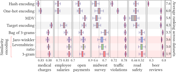
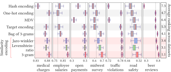
Gradient                                                                                                                                boosted trees                                                                                                                                 Ridge                                                                                                                                regression                                                                                                                                

Figure 2: Performance of different encoding methods. Upper figure: gradient boosting; Lower figure: ridge regression. Each box-plot summarizes the prediction scores of 100 random splits (with 80% of the samples for training and 20% for testing). For all datasets, the prediction score is upper bounded by $1$ (a higher score means a better prediction). The right side of the figure indicates the average ranking across datasets for each method. The vertical dashed line indicates the median value of the one-hot encoding method.

First, we benchmarked the similarity encoding with one-hot encoding and other commonly used methods. Each box-plot in Figure 2 contains the prediction scores of 100 random splits of the data (80% of the samples for training and 20% for testing) using gradient boosted trees and ridge regression. The right side of each plot shows the average ranking of each method across datasets in terms of the median value of the respective box-plots

In general, similarity encoding methods have the best results in terms of the average ranking across datasets, with 3-gram being the one that performs the best for both classifiers (for Ridge, 3-gram similarity is the best method on every dataset). On the contrary, the hashing encoder has the worst performance. Target and MDV encodings perform well (in particular with gradient boosting), considering that the dimension of the feature vector is equal to $1$ for regression and binary classification, and to the number of classes for multiclass classification (which goes up to 104 classes for the beer reviews dataset).

Figure 3: Scores with different classifiers Comparison between one-hot and 3-gram similarity encoding. Each box-plot corresponds to 100 random splits with 20% of the samples for the testing set. The right side of the figure indicates the average ranking across datasets for each method in terms of the median value of the 3-gram similarity.

Figure 3 shows the difference in score between one-hot and similarity encoding for different regressors/classifiers: standard linear methods, ridge and logistic regression with internal cross-validation of the regularization parameter, and also the tree-based methods, random forest and gradient boosting. The average ranking is computed with respect to the 3-gram similarity scores. The medical charges and employee salaries datasets do not have scores for the logistic model because their prediction task is a regression problem.

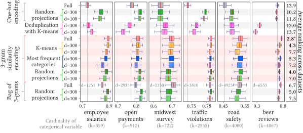
Gradient                                                                                                                                   boosted trees                                                                                                                                   

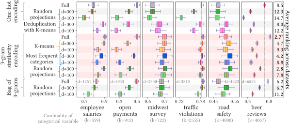
Ridge                                                                                                                                   regression                                                                                                                                   

Figure 4: Performance with different dimensionality reduction methods. $Full$ denotes the encoding without dimensionality reduction and $d$ the dimension of the reduction. Each box-plot corresponds to 100 random splits with 80% of the samples for the training set and 20% for the testing set. The right side of the plot indicates the average ranking across datasets for each method (^∗ denotes the best average ranking).

Figure 4 shows prediction results of different dimensionality reduction methods applied six of our seven datasets (medical charges was excluded from the figure because of its smaller cardinality in comparison with the other datasets). For dimension reduction, we investigated i) random projections, ii) encoding with similarities to the most frequent categories, iii) encoding with similarities to categories closest to the centers of a k-means clustering, and iv) one-hot encoding after merging categories with a k-means clustering, which is a simple form of deduplication. The latter method enables bridging the gap with the deduplication literature: we can compare merging entities before statistical learning to expressing their similarity using the same similarity measure.

6 Discussion

Encoding categorical textual variables in dirty tables has not been studied much in the statistical-learning literature. Yet it is a common hurdle in many application settings. This paper shows that there is room for improvement upon the standard practice of one-hot encoding by accounting for similarities across the categories. We studied similarity encoding, which is a very simple generalization of the one-hot encoding method.

An important contribution of this paper is the empirical benchmarks on dirty tables. We selected seven real-world datasets containing at least one dirty categorical variable with high-cardinality (see Table 2). These datasets are openly available, and we hope that they will foster more research on dirty categorical variables. By their diversity, they enable exploring the trade-offs of encoding approaches and conclude on generally-useful defaults.

The 3-gram similarity appears to be a good choice, outperforming similarities typically used for entity resolution such as Jaro-Winkler and Levenshtein-ratio (Figure 2). A possible reason for the success of 3-gram is visible in the histogram of the similarities across classes (Figure 5). For all datasets, 3-gram has the smallest median values, and assigns 0 similarity to many pairs of categories. This allows better separation of similar and dissimilar categories, e.g., ‘midwest’ and ‘mid west’ as opposed to ‘southern’. 3-gram similarity also outperforms the bag of 3-grams. Indeed, similarity encoding implicitly defines the following kernel between two observations:

$$\langle d^{i},d^{j}\rangle_{\text{sim}}=\sum_{l=1}^{k}\text{sim}(d^{i},d_{l})\,\text{sim}(d^{j},d_{l})$$ (12)

Hence, it projects on a dictionary of reference n-grams and gives more importance to the n-grams that best capture the similarity between categories.

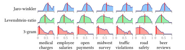
Figure 5: Histogram of pairwise similarity between categories for different string similarity metrics. 10,000 pairs of categories were randomly generated for each dataset (y-axis in logarithmic scale). The red bar denotes the median value for each distribution. Note that medical charge, employee salaries and traffic violations present bimodal distributions.

Figure 5 also reveals that three of the seven datasets (medical charge, employee salaries and traffic violations) display a bimodal distribution in similarities. On these datasets, similarity encoding brings the largest gains over one-hot encoding (Figure 2). In these situations, similarity encoding is particularly useful as it gives a vector representation in which a non-negligible number of category pairs are close to each other.

Performance comparisons with different classifiers (linear models and tree-based models in Figure 3) suggest that 3-gram similarity reduces the gap between models by giving a better vector representation of the categories. Note that in these experiments linear models slightly outperformed tree-based models, however we did not tune the hyper parameters of the tree learners.

While one-hot encoding can be expressed as a sparse matrix, a drawback of similarity encoding is that it creates a dense feature matrix, leading to increased memory and computational costs. Dimensionality reduction of the resulting matrix maintains most of the benefits of similarity encoding (Figure 4) even with a strong reduction ($d$$=$$100$). It greatly reduces the computational cost: fitting the models on our benchmark datasets takes on the order of seconds or minutes on commodity hardware (see Table 3 in the appendix). Note that on some datasets, a random projection of one-hot encoded vectors improves prediction for gradient boosting. We interpret this as a regularization that captures some semantic links across the categories, as with LSA. When more than one categorical variable is present, a related approach would be to use Correspondence Analysis shyu2005handling , which also seeks a low-rank representation as it can be interpreted as a weighted form of PCA for categorical data. Here we focus on methods that encode a single categorical variable.

The dimension reduction approaches that we have studied can be applied in an online learning setting: they either select a small number prototype categories, or perform a random projection. Hence, the approach can be applied on datasets that do not fit in memory.

Classic encoding methods are hard to apply in incremental machine-learning settings. Indeed, new samples with new categories require recomputation of the encoding representation, and hence retrain the model from scratch. This is not the case of similarity encoding because new categories are naturally encoded without creating collisions. We have shown the power of a straightforward strategy based on selecting 100 prototypes on subsampled data, for instance with k-means clustering. Most importantly, no data cleaning on categorical variables is required to apply our methodology. Scraped data for commercial or marketing applications are good candidates to benefit from this approach.

7 Conclusion

Similarity encoding, a generalization of the one-hot encoding method, allows a better representation of categorical variables, especially in the presence of dirty or high-cardinality categorical data. Empirical results on seven real-world datasets show that 3-gram similarity is a good choice to capture morphological resemblance between categories and to encode new categories that do not appear in the testing set. It improves prediction of the associated supervised learning task without any prior data-cleaning step. Similarity encoding also outperforms representing categories via “bags of n-grams” of the associated strings. Its benefits carry over even with strong dimensionality reduction based on cheap operations such as random projections. This methodology can be used in online-learning settings, and hence can lead to tractable analysis on very large datasets without data cleaning. This paper only scratches the surface of statistical learning on non-curated tables, a topic that has not been studied much. We hope that the benchmarks datasets will foster more work on this subject.

8 Appendix

8.1 Datasets description.

Medical Charges.

Inpatient discharges for Medicare beneficiaries: utilization, payment, and hospital-specific charges for more than 3,000 U.S. hospitals. Sample size (random subsample): 100,000. Target variable (regression): ‘Average total payments’ (what Medicare pays to the provider). Selected categorical variable: ‘Medical procedure’ (cardinality: 3023). Other explanatory variables: ‘State’ (categorical), ‘Average Covered Charges’ (numerical).

Employee Salaries.

Annual salary information (year 2016) for employees of Montgomery County, Maryland. Sample size: 9,200. Target variable (regression): ‘Current Annual Salary’. Selected cat. variable: ‘Employee Position Title’ (cardinality: 385). Other explanatory variables: ‘Gender’ (c), ‘Department Name’ (c), ‘Division’ (c), ‘Assignment Category’ (c), ‘Date First Hired’ (n).

Open Payments.

Payments given by healthcare manufacturing companies to medical doctors or hospitals. Sample size (random subsample): 100,000 (year 2013). Target variable (binary classification): ‘Status’ (if the payment was made under a research protocol) Selected categorical variable: ‘Company name’ (card.: 973). Other explanatory variables: ‘Amount of payments in US dollars’ (n), ‘Dispute’ (whether the physician refused the payment) (c).

Midwest Survey.

Survey to know if people self-identify as Midwesterners. Sample size: 2,778. Target variable (multiclass-clf): ‘Location (Census Region)’ (10 classes). Selected categorical variable: ‘In your own words, what would you call the part of the country you live in now?’ (cardinality: 1,009). Other explanatory variables: ‘Personally identification as a Midwesterner?’, ‘Gender’, ‘Age’, ‘Household Income’, ‘Education’, ‘Illinois (IL) in the Midwest?’, ‘IN?’, ‘IA?’, ‘KS?’, ‘MI?’, ‘MN?’, ‘MO?’, ‘NE?’, ‘ND?’, ‘OH?’, ‘SD?’, ‘WI?’, ‘AR?’, ‘CO?’, ‘KY?’, ‘OK?’, ‘PA?’, ’WV?’, ’MT?’, ‘WY?’.

Traffic Violations.

Traffic information from electronic violations issued in the Montgomery County of Maryland. Sample size (random subsample): 100,000. Target variable (multiclass-clf): ‘Violation type’ (4 classes). Selected categorical variable: ‘Description’ (card.: 3,043). Other explanatory variables: ‘Belts’ (c), ‘Property Damage’ (c), ‘Fatal’ (c), ‘Commercial license’ (c), ‘Hazardous materials’ (c), ‘Commercial vehicle’ (c), ‘Alcohol’ (c), ‘Work zone’ (c), ‘Year’ (n), ‘Race’ (c), ‘Gender’ (c), ‘Arrest type’ (c).

Road Safety.

Data reported to the police about the circumstances of personal injury road accidents in Great Britain from 1979, and the maker and model information of vehicles involved in the respective accident. Sample size (random subsample): 10,000. Target variable (binary-clf): ‘Sex of Driver’. Selected categorical variable: ‘Model’ (card.: 4617) Other variables: ‘Make’ (c).

Beer Reviews.

More than 1.5 million beer reviews. Each review includes ratings in terms of five “aspects”: appearance, aroma, palate, taste, and overall impression. Sample size (random subsample): 10,000. Target variable (multiclass-clf): ‘Beer style’ (104 classes). Selected cat. variable: ‘Beer name’ (card.: 4634) Other variables (numerical): ‘Aroma’, ‘Appearance’, ‘Palate’, ‘Taste’.

8.2 Technical details on the experiments: prediction pipeline

Sample size.

To reduce computational time on the training step, we limited the number of samples to 100,000 for large datasets. For the two datasets with the largest cardinality of the respective categorical variable (beer reviews and road safety), the sample size was set to 10,000.

Data preprocessing.

We removed rows with missing values in the target variable or in any explanatory variable other than the selected categorical variable, for which we replaced missing entries by the string ‘nan’. The only additional preprocessing for the categorical variable was to transform all entries to lower case. We standardized every column of the feature matrix to a unit variance.

Cross-validation.

For every prediction task, we made 100 random splits of the data, with 20% of samples for testing at each time. In the case of binary-class classification, we performed stratified randomization.

Performance metrics.

Depending on the type of prediction task, we used different scores to evaluate the performance of the supervised learning problem: for regression, we used the $R^{2}$ score; for binary classification, the average precision; and for multiclass classification, the accuracy score.

Parametrization of classifiers.

We used the scikit-learn implementation of the following methods: LogisticRegressionCV, RidgeCV (CV denotes internal cross-validation for the regularization parameter), GradientBoosting and RandomForest. In general, the default parameters were used, with the following exceptions: i) for ensemble methods, the number of estimators was set to 100; ii) For ridge regression, we use internal 3-fold cross-validation to set the regularization parameter; iii) when possible, we set class_weight=‘balanced’. Default parameter settings can be found at http://scikit-learn.org/.

Table 3: Average prediction times (in seconds) for the 3-gram similarity encoding with k-means for dimensionality reduction.

	Gradient boosting				Ridge CV
Dataset	Full	d=300	d=100	d=30	Full	d=300	d=100	d=30
Medical charges	311	-	156	74	2.5	-	2.3	2.8
Employee salaries	69	50	47	37	3.9	2.8	2.6	1.6
Open payments	1,116	393	125	45	61.0	12.7	2.2	0.7
Midwest survey	104	42	14	8.6	1.9	0.4	0.1	0.1
Traffic violations	12,165	1,686	686	262	116.6	7.1	2.3	1.1
Road safety	211	30	10	6	78.2	1.5	0.6	0.4
Beer reviews	14,214	2,260	809	436	302.7	2.0	0.6	0.5